Degradation-Aware Unfolding Half-Shuffle Transformer for Spectral Compressive Imaging

Abstract

In coded aperture snapshot spectral compressive imaging (CASSI) systems, hyperspectral image (HSI) reconstruction methods are employed to recover the spatial-spectral signal from a compressed measurement. Among these algorithms, deep unfolding methods demonstrate promising performance but suffer from two issues. Firstly, they do not estimate the degradation patterns and ill-posedness degree from CASSI to guide the iterative learning. Secondly, they are mainly CNN-based, showing limitations in capturing long-range dependencies. In this paper, we propose a principled Degradation-Aware Unfolding Framework (DAUF) that estimates parameters from the compressed image and physical mask, and then uses these parameters to control each iteration. Moreover, we customize a novel Half-Shuffle Transformer (HST) that simultaneously captures local contents and non-local dependencies. By plugging HST into DAUF, we establish the first Transformer-based deep unfolding method, Degradation-Aware Unfolding Half-Shuffle Transformer (DAUHST), for HSI reconstruction. Experiments show that DAUHST surpasses state-of-the-art methods while requiring cheaper computational and memory costs. Code and models are publicly available at https://github.com/caiyuanhao1998/MST

1 Introduction

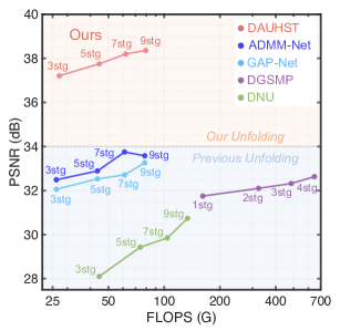
Figure 1: PSNR-FLOPS comparisons of DAUHST and SOTA unfolding methods.

Hyperspectral images (HSIs) have more spectral bands than normal RGB images to store more detailed information. Thus, HSIs are widely applied in image recognition fauvel2012advances ; maggiori2017recurrent ; zhang2015scene , object detection ot_1 ; ot_2 ; ot_3 , tracking fu2016exploiting ; uzkent2016real ; uzkent2017aerial , medical image processing mi_1 ; mi_2 ; mi_3 , remote sensing rs_1 ; rs_2 ; rs_3 ; rs_4 , etc. To obtain HSIs, traditional imaging systems use spectrometers to scan the scenes along the spectral or spatial dimensions, usually requiring a long time. These imaging systems fail to capture dynamic objects. Recently, snapshot compressive imaging (SCI) systems sci_1 ; sci_2 ; sci_3 ; sci_5 ; sci_6 ; yuan2015compressive ; ma2021led have been developed to capture HSIs at video rate. Among these SCI systems, coded aperture snapshot spectral imaging (CASSI) sci_2 ; tsa_net ; gehm2007single stands out for its impressive performance. CASSI uses a coded aperture and a disperser to modulate the HSI signal at different wavelengths, and then mixes all modulated signal to generate a 2D compressed measurement. Subsequently, HSI restoration methods are employed to solve the CASSI inverse problem, i.e., restore the HSIs from the measurement. These methods are divided into four categories.

(i) Model-based methods sci_2 ; sparse_1 ; desci ; non_local_1 ; non_local_2 ; gap_tv ; tra_rela_1 ; gradient rely on hand-crafted image priors, e.g., total variation gap_tv , sparsity sci_2 ; sparse_1 , low-rank desci , etc. These methods have theoretically proven properties and can be interpreted. Yet, these methods need manual parameter tweaking, which slows down reconstruction. Also, they suffer from limited representation capacity and generalization ability.

(ii) Plug-and-play (PnP) algorithms pnp_3 ; pnp_1 ; pnp_2 ; self ; zheng2021deep ; yuan2021plug plug pre-trained denoising networks into traditional model-based methods pnp_2 ; qiao2020deep to solve the HSI reconstruction problem. Nonetheless, the pre-trained networks in PnP methods are fixed without re-training, therefore limiting the performance.

(iii) End-to-end (E2E) algorithms employ a powerful model, usually a convolutional neural network (CNN) mi_3 ; tsa_net ; hdnet ; lambda , to learn the E2E mapping function from a measurement to the desired HSIs. E2E methods enjoy the power of deep learning. However, they learn a brute-force mapping from the compressed measurement to the underlying spectral images, thereby ignoring the working principles of CASSI systems. They come without theoretically proven properties, interpretability Yuan_review , and flexibility because the imaging models widely differ from each other for various hardware systems.

(iv) Deep unfolding methods dnu ; hssp ; gapnet ; admm-net ; gsm ; fu2021bidirectional ; herosnet adopt a multi-stage network to map the measurement into the HSI cube. Each stage usually includes two phases, i.e., linear projection followed by passing the signal through a single-stage network that learns the underlying denoiser prior. In deep unfolding methods, the network architecture is intuitively interpretable by explicitly characterizing the image priors and the system imaging model. Besides, these methods also enjoy the power of deep learning and thus have great potential. Yet, this potential has not been fully explored.

Existing deep unfolding algorithms suffer from two issues. (a) The iterative learning is highly related to the CASSI system. However, current unfolding methods do not estimate CASSI degradation patterns and ill-posedness degree to adjust the linear projection and denoising network in each iteration. (b) Existing deep unfolding methods are mainly CNN-based, therefore showing limitations in capturing non-local self-similarity and long-range dependencies, both critical for HSI reconstruction.

Recently, the emerging Transformer vaswani2017attention has provided a solution to tackle the drawbacks of CNN. Due to its strong capability in modeling the interactions of non-local spatial regions, Transformer has been widely applied in image classification liu2021swin ; arnab2021vivit ; global_msa ; tc_2 ; tc_3 ; xcit ; crossvit , object detection de_detr ; to_1 ; liu2021swin ; DETR ; dy_detr ; to_2 ; to_5 , semantic segmentation liu2021swin ; tc_3 ; ts_1 ; cao2021swin ; ts_2 ; ts_3 ; ts_4 , human pose estimation tokenpose ; transpose ; rsn ; prtr ; th_1 ; th_2 ; th_3 , image restoration ipt ; swinir ; uformer ; vsrt ; fgst ; mst ; mst_pp ; cst ; pngan ; rformer , etc. Yet, the use of Transformer is confronted with two main issues. (a) The computational complexity of global Transformer global_msa is quadratic to the spatial dimensions. This nontrivial cost is sometimes unaffordable. (b) The receptive fields of local Transformer liu2021swin are limited within position-specific windows. As a result, some tokens with highly-related contents can not match each other when computing the self-attention.

To address the above problems, in this paper, we firstly formulate a principled Degradation-Aware Unfolding Framework (DAUF) based on maximum a posteriori (MAP) theory for HSI reconstruction. Different from previous deep unfolding methods, our DAUF implicitly estimates informative parameters from the degraded compressed measurement and the physical mask used in the modulation. Then DAUF feeds the parameters, which capture key cues of CASSI degradation patterns and ill-posedness degree, into each iteration to adaptively scale the linear projection and provide the noise level information for the denoising network. Secondly, we design a novel Half-Shuffle Transformer (HST) as the denoiser prior in each iteration. Our HST can jointly extract local contextual information and model non-local dependencies, while requiring much cheaper computational costs than global Transformer. We achieve this by customizing a Half-Shuffle Multi-head Self-Attention (HS-MSA) mechanism that composes the basic unit of HST. More specifically, our HS-MSA has two branches, i.e., $local~{}branch$ and $non$-$local~{}branch$. The $local~{}branch$ calculates the self-attention within the local window while the $non$-$local~{}branch$ shuffles the tokens and captures cross-window interactions. We plug HST into DAUF to establish an iterative architecture, Degradation-Aware Unfolding Half-Shuffle Transformer (DAUHST). With the proposed techniques, DAUHST models dramatically outperform state-of-the-art (SOTA) deep unfolding methods with the same number of stages by over 4 dB, as shown in Fig. 1.

In a nutshell, our contributions can be summarized as follows:

(i) We formulate a principled MAP-based unfolding framework DAUF for HSI reconstruction.

(ii) We propose a novel Transformer HST and plug it into DAUF to establish DAUHST. To the best of our knowledge, DAUHST is the first Transformer-based deep unfolding method for HSI restoration.

(iii) DAUHST outperforms SOTA methods by a large margin while requiring cheaper computational and memory costs. Besides, DAUHST yields more visually pleasant results in real HSI reconstruction.

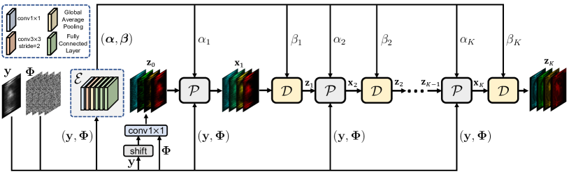
Figure 2: The architecture of our DAUF with $K$ stages (iterations). $\mathcal{E}$ estimates informative parameters from the compressed measurement $\mathbf{y}$ and sensing matrix $\mathbf{\Phi}$. The estimated parameters $\boldsymbol{\alpha}$ and $\boldsymbol{\beta}$ are fed into each stage of subsequent iterative learning. $\mathcal{P}$ and $\mathcal{D}$ denote the linear projection and denoising network in each stage.

2 Proposed Method

2.1 Degradation Model of CASSI

In CASSI, we denote the vectorized measurement as $\mathbf{y}\in\mathbb{R}^{n}$, where $n$ = $H(W+d(N_{\lambda}-1))$. $H$, $W$, $d$, and $N_{\lambda}$ denote the HSI’s height, width, shifting step in dispersion, and total number of wavelengths. Given the vectorized shifted HSI signal $\mathbf{x}\in\mathbb{R}^{nN_{\lambda}}$ and the sensing matrix $\mathbf{\Phi}\in\mathbb{R}^{n\times nN_{\lambda}}$ that is determined by the physical mask, the degradation model of CASSI can be formulated as

$$\mathbf{y}=\mathbf{\Phi}\mathbf{x}+\mathbf{n},$$ (1)

where $\mathbf{n}\in\mathbb{R}^{n}$ represents the vectorized imaging noise on the measurement. As analyzed in  Tropp07ITT ; Donoho06ITT ; jalali2019snapshot , $\mathbf{\Phi}$ is a fat, sparse, and highly structured matrix that is hard to handle. Please refer to the supplementary material for details about the mathematical model of CASSI. Then the task of HSI reconstruction is given $\mathbf{y}$ (captured by the camera) and $\mathbf{\Phi}$ (calibrated based on pre-design), solving $\mathbf{x}$.

2.2 Degradation-Aware Unfolding Framework

Previous unfolding frameworks dnu ; hssp ; gapnet ; admm-net do not estimate the CASSI degradation patterns to adjust the iterative learning. To alleviate this limitation, we formulate a principled Degradation-Aware Unfolding Framework (DAUF) as depicted in Fig. 2. DAUF starts from the MAP theory. In particular, the original HSI signal could be estimated by minimizing the following energy function as

$$\mathbf{\hat{x}}=\text{arg}~{}\underset{\mathbf{x}}{\text{min}}~{}~{}\frac{1}{2}||\mathbf{y}-\mathbf{\Phi}\mathbf{x}||^{2}+\tau R(\mathbf{x}),$$ (2)

where $\frac{1}{2}||\mathbf{y}-\mathbf{\Phi}\mathbf{x}||^{2}$ is the data fidelity term, $R(\mathbf{x})$ is the image prior term, and $\tau$ is a hyperparameter balancing the importance. By introducing an auxiliary variable $\mathbf{z}$, Eq. (2) can be reformulated as

$$\mathbf{\hat{x}}=\text{arg}~{}\underset{\mathbf{x}}{\text{min}}~{}~{}\frac{1}{2}||\mathbf{y}-\mathbf{\Phi}\mathbf{x}||^{2}+\tau R(\mathbf{z}),~{}~{}~{}~{}s.t.~{}~{}\mathbf{z}=\mathbf{x}.$$ (3)

This is a constrained optimization problem. To obtain an unfolding inference, we adopt half-quadratic splitting (HQS) algorithm for its simplicity and fast convergence. Then Eq. (3) is solved by minimizing

$$\mathcal{L}_{\mu}(\mathbf{x},\mathbf{z})=\frac{1}{2}||\mathbf{y}-\mathbf{\Phi}\mathbf{x}||^{2}+\tau R(\mathbf{z})+\frac{\mu}{2}||\mathbf{z}-\mathbf{x}||^{2},$$ (4)

where $\mu$ is a penalty parameter that forces $\mathbf{x}$ and $\mathbf{z}$ to approach the same fixed point. Subsequently, Eq. (4) can be solved by decoupling $\mathbf{x}$ and $\mathbf{z}$ into the following two iterative sub-problems as

$$\mathbf{x}_{k+1}=\text{arg}~{}\underset{\mathbf{x}}{\text{min}}~{}~{}||\mathbf{y}-\mathbf{\Phi}\mathbf{x}||^{2}+\mu||\mathbf{x}-\mathbf{z}_{k}||^{2}~{},~{}~{}~{}\mathbf{z}_{k+1}=\text{arg}~{}\underset{\mathbf{z}}{\text{min}}~{}~{}\frac{\mu}{2}||\mathbf{z}-\mathbf{x}_{k+1}||^{2}+\tau R(\mathbf{z}),$$ (5)

where $k=0,1,~{}...~{},K-1$ indexes the iteration. Note that the data fidelity term is associated with a quadratic regularized least-squares problem, i.e., $\mathbf{x}_{k+1}$ in Eq. (5). It has a closed-form solution as

$$\mathbf{x}_{k+1}=(\mathbf{\Phi}^{\mathsf{T}}\mathbf{\Phi}+\mu\mathbf{I})^{-1}(\mathbf{\Phi}^{\mathsf{T}}\mathbf{y}+\mu\mathbf{z}_{k}),$$ (6)

where $\mathbf{I}$ is an identity matrix. Since $\mathbf{\Phi}$ is a fat matrix, $(\mathbf{\Phi}^{\mathsf{T}}\mathbf{\Phi}+\mu\mathbf{I})$ will be large and thus we simplify the computation of the inverse problem $(\mathbf{\Phi}^{\mathsf{T}}\mathbf{\Phi}+\mu\mathbf{I})^{-1}$ by the matrix inversion formula as

$$(\mathbf{\Phi}^{\mathsf{T}}\mathbf{\Phi}+\mu\mathbf{I})^{-1}=\mu^{-1}\mathbf{I}-\mu^{-1}\mathbf{\Phi}^{\mathsf{T}}(\mathbf{I}+\mathbf{\Phi}\mu^{-1}\mathbf{\Phi}^{\mathsf{T}})^{-1}\mathbf{\Phi}\mu^{-1}.$$ (7)

By plugging Eq. (7) into Eq. (6), we can reformulate Eq. (6) as

$$\mathbf{x}_{k+1}=\frac{\mathbf{\Phi}^{\mathsf{T}}\mathbf{y}+\mu\mathbf{z}_{k}}{\mu}-\frac{\mathbf{\Phi}^{\mathsf{T}}(\mathbf{I}+\mathbf{\Phi}\mu^{-1}\mathbf{\Phi}^{\mathsf{T}})^{-1}\mathbf{\Phi}\mathbf{\Phi}^{\mathsf{T}}\mathbf{y}}{\mu^{2}}-\frac{\mathbf{\Phi}^{\mathsf{T}}(\mathbf{I}+\mathbf{\Phi}\mu^{-1}\mathbf{\Phi}^{\mathsf{T}})^{-1}\mathbf{\Phi}\mathbf{z}_{k}}{\mu}~{}.$$ (8)

In CASSI systems, $\mathbf{\Phi}\mathbf{\Phi}^{\mathsf{T}}$ is a diagonal matrix which can be defined as $\mathbf{\Phi}\mathbf{\Phi}^{\mathsf{T}}\stackrel{{\scriptstyle\rm def}}{{=}}{\rm diag}\{\psi_{1},\dots,\psi_{n}\}$. By plugging $\mathbf{\Phi}\mathbf{\Phi}^{\mathsf{T}}$ into $(\mathbf{I}+\mathbf{\Phi}\mu^{-1}\mathbf{\Phi}^{\mathsf{T}})^{-1}$ and $(\mathbf{I}+\mathbf{\Phi}\mu^{-1}\mathbf{\Phi}^{\mathsf{T}})^{-1}\mathbf{\Phi}\mathbf{\Phi}^{\mathsf{T}}$, we obtain:

$$(\mathbf{I}+\mathbf{\Phi}\mu^{-1}\mathbf{\Phi}^{\mathsf{T}})^{-1} =\text{diag}\Big{\{}\frac{\mu}{\mu+\psi_{1}},...~{},\frac{\mu}{\mu+\psi_{n}}\Big{\}},$$ (9)

$$(\mathbf{I}+\mathbf{\Phi}\mu^{-1}\mathbf{\Phi}^{\mathsf{T}})^{-1}\mathbf{\Phi}\mathbf{\Phi}^{\mathsf{T}} =\text{diag}\Big{\{}\frac{\mu\psi_{1}}{\mu+\psi_{1}},...~{},\frac{\mu\psi_{n}}{\mu+\psi_{n}}\Big{\}}.$$

Let $\mathbf{y}\stackrel{{\scriptstyle\rm def}}{{=}}[y_{1},\dots,y_{n}]^{\mathsf{T}}$ and $[\mathbf{\Phi}\mathbf{z}_{k}]_{i}$ denotes the $i$-th element of $\mathbf{\Phi}\mathbf{z}_{k}$. We plug Eq. (9) into Eq. (8) as

$$\mathbf{x}_{k+1} =\frac{\mathbf{\Phi}^{\mathsf{T}}\mathbf{y}}{\mu}+\mathbf{z}_{k}-\frac{1}{\mu}\mathbf{\Phi}^{\mathsf{T}}\Big{[}\frac{y_{1}\psi_{1}+\mu[\mathbf{\Phi}\mathbf{z}_{k}]_{1}}{\mu+\psi_{1}},...~{},\frac{y_{n}\psi_{n}+\mu[\mathbf{\Phi}\mathbf{z}_{k}]_{n}}{\mu+\psi_{n}}\Big{]}^{\mathsf{T}}$$ (10)

$$=\mathbf{z}_{k}+\mathbf{\Phi}^{\mathsf{T}}\Big{[}\frac{y_{1}-[\mathbf{\Phi}\mathbf{z}_{k}]_{1}}{\mu+\psi_{1}},...~{},\frac{y_{n}-[\mathbf{\Phi}\mathbf{z}_{k}]_{n}}{\mu+\psi_{n}}\Big{]}^{\mathsf{T}}.$$

Note that $\{y_{i}-[\mathbf{\Phi}\mathbf{z}_{k}]_{i}\}_{i=1}^{n}$ can be directly updated by $\mathbf{y}-\mathbf{\Phi}\mathbf{z}_{k}$, and $\{\psi_{i}\}_{i=1}^{n}$ is pre-calculated and stored in $\mathbf{\Phi}\mathbf{\Phi}^{\mathsf{T}}$. Thus, by element-wise computation in Eq. (10), $\mathbf{x}_{k+1}$ can be updated very efficiently. According to Eq. (5), the penalty parameter $\mu$ should be large enough so that $\mathbf{x}$ and $\mathbf{z}$ can approach approximately the same fixed point. This indicates that $\mu$ controls the convergence and output of each iteration. Thus, instead of manually tweaking $\mu$, we set $\mu$ as a series of iteration-specific parameters to be automatically estimated from the CASSI system. We denote $\mu$ in the $k$-th iteration as $\mu_{k}$.

Returning to Eq. (5), we also set $\tau$ as iteration-specific parameters and $\mathbf{z}_{k+1}$ can be reformulated as

$$\mathbf{z}_{k+1}=\text{arg}~{}\underset{\mathbf{z}}{\text{min}}~{}~{}\frac{1}{2(\sqrt{\tau_{k+1}/\mu_{k+1}})^{2}}~{}||\mathbf{z}-\mathbf{x}_{k+1}||^{2}+R(\mathbf{z}).$$ (11)

From the perspective of Bayesian probability, Eq. (11) is equivalent to denoising image $\mathbf{x}_{k+1}$ with a Gaussian noise at level $\sqrt{\tau_{k+1}/\mu_{k+1}}$ pnp_3 . To conveniently solve Eq. (11), we set $\frac{1}{(\sqrt{\tau_{k+1}/\mu_{k+1}})^{2}}=\mu_{k+1}/\tau_{k+1}$ as parameters to be estimated from CASSI. Let $\alpha_{k}\stackrel{{\scriptstyle\rm def}}{{=}}\mu_{k}$, $\boldsymbol{\alpha}\stackrel{{\scriptstyle\rm def}}{{=}}[\alpha_{1},...,\alpha_{K}]$, $\beta_{k}\stackrel{{\scriptstyle\rm def}}{{=}}\mu_{k}/\tau_{k}$, and $\boldsymbol{\beta}\stackrel{{\scriptstyle\rm def}}{{=}}[\beta_{1},...,\beta_{K}]$. Then we can formulate our DAUF as an iterative scheme:

$$(\boldsymbol{\alpha},\boldsymbol{\beta})=\mathcal{E}(\mathbf{y},\mathbf{\Phi}),~{}~{}~{}~{}\mathbf{x}_{k+1}=\mathcal{P}(\mathbf{y},\mathbf{z}_{k},\alpha_{k+1},\mathbf{\Phi}),~{}~{}~{}~{}\mathbf{z}_{k+1}=\mathcal{D}(\mathbf{x}_{k+1},\beta_{k+1}),$$ (12)

where $\mathcal{E}$ denotes the parameter estimator that takes the compressed measurement $\mathbf{y}$ and the sensing matrix $\mathbf{\Phi}$ of the CASSI system as inputs, $\mathcal{P}$ equivalent to Eq. (10) denotes the linear projection, and $\mathcal{D}$ represents the Gaussian denoiser solving Eq. (11). $\mathbf{z}_{0}$ is initialized by passing the shifted $\mathbf{y}$ concatenated with $\mathbf{\Phi}$ through a $conv1\times 1$ (convolution with 1$\times$1 kernel). Fig. 2 shows the architecture of $\mathcal{E}$. It consists of a $conv1\times 1$, a strided $conv3\times 3$, a global average pooling, and three fully connected layers. Through $\mathcal{E}$, DAUF captures critical cues from CASSI by learning the degradation patterns and ill-posedness degree caused by the mask-modulation and dispersion-integration. Parameters $\boldsymbol{\alpha}$ and $\boldsymbol{\beta}$ estimated by $\mathcal{E}$ direct the iterative learning by adaptively scaling the linear projection in Eq. (10) and providing noise level information for the denoiser prior in Eq. (11).

2.3 Half-Shuffle Transformer

When designing the denoiser prior, previous deep unfolding methods dnu ; hssp ; gapnet ; admm-net mainly adopt CNNs, showing limitations in capturing long-range dependencies. Directly applying local and global Transformers will encounter two problems, i.e., limited receptive fields and nontrivial computational costs. To address these challenges, we propose Half-Shuffle Transformer (HST) to play the role of $\mathcal{D}$.

Network Architecture. As shown in Fig. 3 (a), HST adopts a three-level U-shaped structure built by the basic unit Half-Shuffle Attention Block (HSAB). Firstly, HST uses a $conv3\times 3$ to map reshaped $\mathbf{x}_{k}$ concatenated with stretched $\beta_{k}$ into feature $\mathbf{X}_{0}\in\mathbb{R}^{H\times\hat{W}\times C}$, where $\hat{W}$ = $W+d(N_{\lambda}-1)$. Secondly, $\mathbf{X}_{0}$ passes through the encoder, bottleneck, and decoder to be embedded into deep feature $\mathbf{X}_{d}\in\mathbb{R}^{H\times\hat{W}\times C}$. Each level of the encoder or decoder contains an HSAB and a resizing module. In Fig. 3 (b), HSAB consists of two layer normalization (LN), an HS-MSA, and a Feed-Forward Network (FFN) that is detailed in Fig. 3 (c). The downsampling and upsampling modules are strided $conv4\times 4$ and $deconv2\times 2$. Finally, a $conv3\times 3$ operates on $\mathbf{X}_{d}$ to generate a residual image $\mathbf{R}\in\mathbb{R}^{H\times\hat{W}\times N_{\lambda}}$. The output denoised image $\mathbf{z}_{k}$ is obtained by the sum of $\mathbf{x}_{k}$ and reshaped $\mathbf{R}$.

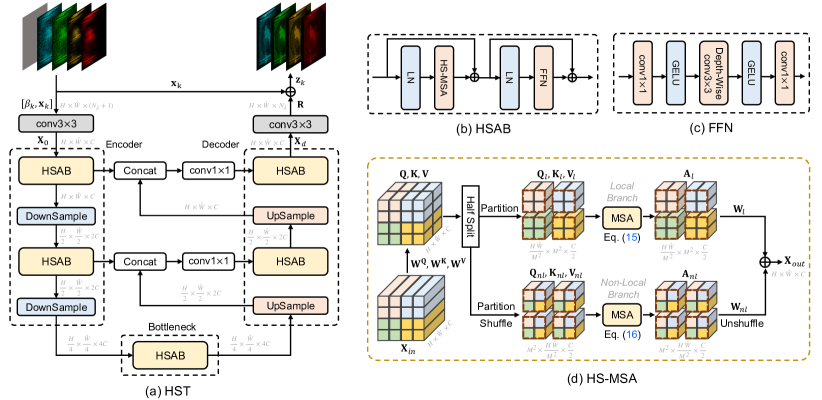
Figure 3: Diagram of HST. (a) HST adopts a U-shaped structure. (b) HSAB consists of an FFN, an HS-MSA, and two layer normalization. (c) Components of FFN. (d) HS-MSA contains $local~{}branch$ and $non$-$local~{}branch$.

Half-Shuffle Multi-head Self-Attention. The most important element of HSAB is the proposed Half-Shuffle Multi-head Self-Attention (HS-MSA) module. Fig. 3 (d) depicts the HS-MSA used in the first level. The input tokens of HS-MSA are denoted as $\mathbf{X}_{in}\in\mathbb{R}^{H\times\hat{W}\times C}$. Subsequently, $\mathbf{X}_{in}$ is linearly projected into $query$ $\mathbf{Q}\in\mathbb{R}^{H\times\hat{W}\times C}$, $key~{}\mathbf{K}\in\mathbb{R}^{H\times\hat{W}\times C}$, and $value$ $\mathbf{V}\in\mathbb{R}^{H\times\hat{W}\times C}$ as

$$\mathbf{Q}=\mathbf{X}_{in}\mathbf{W^{Q}},~{}\mathbf{K}=\mathbf{X}_{in}\mathbf{W^{K}},~{}\mathbf{V}=\mathbf{X}_{in}\mathbf{W^{V}},$$ (13)

where $\mathbf{W^{Q}},\mathbf{W^{K}},\mathbf{W^{V}}\in\mathbb{R}^{C\times C}$ are learnable parameters and biases are omitted for simplification. Our HS-MSA combines the advantages of global MSA global_msa and local window-based MSA liu2021swin , i.e., HS-MSA can jointly capture local contextual information through the local branch and model long-range dependencies through the non-local branch, all while being computationally cheaper than global MSA. Specifically, $\mathbf{Q},\mathbf{K},\mathbf{V}$ are split into two equal parts along the channel dimension as

$$\mathbf{Q}=[\mathbf{Q}_{l},\mathbf{Q}_{nl}],~{}\mathbf{K}=[\mathbf{K}_{l},\mathbf{K}_{nl}],~{}\mathbf{V}=[\mathbf{V}_{l},\mathbf{V}_{nl}],$$ (14)

where $\mathbf{Q}_{l},\mathbf{K}_{l},\mathbf{V}_{l}\in\mathbb{R}^{H\times\hat{W}\times\frac{C}{2}}$ are fed into the $local~{}branch$ to capture local contents, while $\mathbf{Q}_{nl},\mathbf{K}_{nl},\mathbf{V}_{nl}\in\mathbb{R}^{H\times\hat{W}\times\frac{C}{2}}$ pass through the $non$-$local~{}branch$ to model non-local dependencies.

Local Branch. The $local~{}branch$ computes MSA within position-specific windows. As shown in the upper path of Fig. 3 (d), $\mathbf{Q}_{l},\mathbf{K}_{l},\mathbf{V}_{l}$ are partitioned into non-overlapping windows of size $M\times M$. Then they are reshaped into $\mathbb{R}^{\frac{H\hat{W}}{M^{2}}\times M^{2}\times\frac{C}{2}}$. Subsequently, $\mathbf{Q}_{l},\mathbf{K}_{l},\mathbf{V}_{l}$ are split along the channel wise into $h$ heads: $\mathbf{Q}_{l}=[~{}\mathbf{Q}_{l}^{1},\ldots,\mathbf{Q}_{l}^{h}~{}],~{}\mathbf{K}_{l}=[~{}\mathbf{K}_{l}^{1},\ldots,\mathbf{K}_{l}^{h}~{}]$, and $\mathbf{V}_{l}=[~{}\mathbf{V}_{l}^{1},\ldots,\mathbf{V}_{l}^{h}~{}]$. The dimension of each head is $d_{h}=\frac{C}{2h}$. Note that Fig. 3 (d) depicts the situation with $h$ = 1 and some details are omitted for simplification. The local self-attention $\mathbf{A}_{l}^{i}$ is calculated inside each head as

$$\mathbf{A}_{l}^{i}=\text{softmax}(\frac{\mathbf{Q}_{l}^{i}~{}{\mathbf{K}_{l}^{i}}^{\mathsf{T}}}{\sqrt{d_{h}}}+\mathbf{P}_{l}^{i})~{}\mathbf{V}_{l}^{i},~{}~{}~{}i=1,\ldots,h,$$ (15)

where $\mathbf{P}_{l}^{i}\in\mathbb{R}^{M^{2}\times M^{2}}$ are learnable parameters embedding the position information.

Non-local Branch. The $non$-$local~{}branch$ computes cross-window interactions through shuffle operations inspired by ShuffleNet shufflenet . In particular, $\mathbf{Q}_{nl},\mathbf{K}_{nl},\mathbf{V}_{nl}\in\mathbb{R}^{H\times\hat{W}\times\frac{C}{2}}$ are firstly partitioned into non-overlapping windows with size $M\times M$. Then their shapes are transposed from $\mathbb{R}^{\frac{H\hat{W}}{M^{2}}\times M^{2}\times\frac{C}{2}}$ to $\mathbb{R}^{M^{2}\times\frac{H\hat{W}}{M^{2}}\times\frac{C}{2}}$ to shuffle the positions of tokens and establish inter-window dependencies. $\mathbf{Q}_{nl},\mathbf{K}_{nl},\mathbf{V}_{nl}$ are split into $h$ heads: $\mathbf{Q}_{nl}=[~{}\mathbf{Q}_{nl}^{1},\ldots,\mathbf{Q}_{nl}^{h}~{}],~{}\mathbf{K}_{nl}=[~{}\mathbf{K}_{nl}^{1},\ldots,\mathbf{K}_{nl}^{h}~{}],$ and $\mathbf{V}_{nl}=[~{}\mathbf{V}_{nl}^{1},\ldots,\mathbf{V}_{nl}^{h}~{}]$. Then the non-local self-attention $\mathbf{A}_{nl}^{i}$ is computed in each head as

$$\mathbf{A}_{nl}^{i}=\text{softmax}(\frac{\mathbf{Q}_{nl}^{i}~{}{\mathbf{K}_{nl}^{i}}^{\mathsf{T}}}{\sqrt{d_{h}}}+\mathbf{P}_{nl}^{i})~{}\mathbf{V}_{nl}^{i},~{}~{}~{}i=1,\ldots,h,$$ (16)

where $\mathbf{P}_{nl}^{i}\in\mathbb{R}^{\frac{H\hat{W}}{M^{2}}\times\frac{H\hat{W}}{M^{2}}}$ are learnable parameters representing the position embedding. Subsequently, $\mathbf{A}_{nl}^{i}\in\mathbb{R}^{M^{2}\times\frac{H\hat{W}}{M^{2}}\times d_{h}}$ is unshuffled by being transposed to shape $\mathbb{R}^{\frac{H\hat{W}}{M^{2}}\times M^{2}\times d_{h}}$. Then the outputs of $local~{}branch$ in Eq. (15) and $non$-$local~{}branch$ in Eq. (16) are aggregated by a linear projection as

$$\text{HS-MSA}(\mathbf{X}_{in})=\sum\nolimits_{i=1}^{h}\mathbf{A}_{l}^{i}\mathbf{W}_{l}^{i}+\sum\nolimits_{i=1}^{h}\mathbf{A}_{nl}^{i}\mathbf{W}_{nl}^{i},$$ (17)

where $\mathbf{W}_{l}^{i},\mathbf{W}_{nl}^{i}\in\mathbb{R}^{d_{h}\times C}$ refer to learnable parameters. We reshape the result of Eq. (17) to obtain the output $\mathbf{X}_{out}\in\mathbb{R}^{H\times\hat{W}\times C}$. Instead of globally sampling all tokens, HS-MSA builds inter-window correlations by shuffle operations. The self-attention is calculated in the local window but with tokens from non-local regions. Therefore, HS-MSA is much computationally cheaper than global MSA.

Algorithms	Params	GFLOPS	S1	S2	S3	S4	S5	S6	S7	S8	S9	S10	Avg
TwIST twist	-	-	25.16 0.700	23.02 0.604	21.40 0.711	30.19 0.851	21.41 0.635	20.95 0.644	22.20 0.643	21.82 0.650	22.42 0.690	22.67 0.569	23.12 0.669
GAP-TV gap_tv	-	-	26.82 0.754	22.89 0.610	26.31 0.802	30.65 0.852	23.64 0.703	21.85 0.663	23.76 0.688	21.98 0.655	22.63 0.682	23.10 0.584	24.36 0.669
DeSCI desci	-	-	27.13 0.748	23.04 0.620	26.62 0.818	34.96 0.897	23.94 0.706	22.38 0.683	24.45 0.743	22.03 0.673	24.56 0.732	23.59 0.587	25.27 0.721
$\lambda$-Net lambda	62.64M	117.98	30.10 0.849	28.49 0.805	27.73 0.870	37.01 0.934	26.19 0.817	28.64 0.853	26.47 0.806	26.09 0.831	27.50 0.826	27.13 0.816	28.53 0.841
HSSP hssp	-	-	31.48 0.858	31.09 0.842	28.96 0.823	34.56 0.902	28.53 0.808	30.83 0.877	28.71 0.824	30.09 0.881	30.43 0.868	28.78 0.842	30.35 0.852
DNU dnu	1.19M	163.48	31.72 0.863	31.13 0.846	29.99 0.845	35.34 0.908	29.03 0.833	30.87 0.887	28.99 0.839	30.13 0.885	31.03 0.876	29.14 0.849	30.74 0.863
DIP-HSI self	33.85M	64.42	32.68 0.890	27.26 0.833	31.30 0.914	40.54 0.962	29.79 0.900	30.39 0.877	28.18 0.913	29.44 0.874	34.51 0.927	28.51 0.851	31.26 0.894
TSA-Net tsa_net	44.25M	110.06	32.03 0.892	31.00 0.858	32.25 0.915	39.19 0.953	29.39 0.884	31.44 0.908	30.32 0.878	29.35 0.888	30.01 0.890	29.59 0.874	31.46 0.894
DGSMP gsm	3.76M	646.65	33.26 0.915	32.09 0.898	33.06 0.925	40.54 0.964	28.86 0.882	33.08 0.937	30.74 0.886	31.55 0.923	31.66 0.911	31.44 0.925	32.63 0.917
GAP-Net gapnet	4.27M	78.58	33.74 0.911	33.26 0.900	34.28 0.929	41.03 0.967	31.44 0.919	32.40 0.925	32.27 0.902	30.46 0.905	33.51 0.915	30.24 0.895	33.26 0.917
ADMM-Net admm-net	4.27M	78.58	34.12 0.918	33.62 0.902	35.04 0.931	41.15 0.966	31.82 0.922	32.54 0.924	32.42 0.896	30.74 0.907	33.75 0.915	30.68 0.895	33.58 0.918
HDNet hdnet	2.37M	154.76	35.14 0.935	35.67 0.940	36.03 0.943	42.30 0.969	32.69 0.946	34.46 0.952	33.67 0.926	32.48 0.941	34.89 0.942	32.38 0.937	34.97 0.943
MST-L mst	2.03M	28.15	35.40 0.941	35.87 0.944	36.51 0.953	42.27 0.973	32.77 0.947	34.80 0.955	33.66 0.925	32.67 0.948	35.39 0.949	32.50 0.941	35.18 0.948
MST++ mst_pp	1.33M	19.42	35.80 0.943	36.23 0.947	37.34 0.957	42.63 0.973	33.38 0.952	35.38 0.957	34.35 0.934	33.71 0.953	36.67 0.953	33.38 0.945	35.99 0.951
CST-L mst_pp	3.00M	40.01	35.96 0.949	36.84 0.955	38.16 0.962	42.44 0.975	33.25 0.955	35.72 0.963	34.86 0.944	34.34 0.961	36.51 0.957	33.09 0.945	36.12 0.957
BIRNAT birnat	4.40M	2122.66	36.79 0.951	37.89 0.957	40.61 0.971	46.94 0.985	35.42 0.964	35.30 0.959	36.58 0.955	33.96 0.956	39.47 0.970	32.80 0.938	37.58 0.960
DAUHST-2stg	1.40M	18.44	35.93 0.943	36.70 0.946	37.96 0.959	44.38 0.978	34.13 0.954	35.43 0.957	34.78 0.940	33.65 0.950	37.42 0.955	33.07 0.941	36.34 0.952
DAUHST-3stg	2.08M	27.17	36.59 0.949	37.93 0.958	39.32 0.964	44.77 0.980	34.82 0.961	36.19 0.963	36.02 0.950	34.28 0.956	38.54 0.963	33.67 0.947	37.21 0.959
DAUHST-5stg	3.44M	44.61	36.92 0.955	38.52 0.962	40.51 0.967	45.09 0.980	35.33 0.964	36.56 0.965	36.82 0.958	34.74 0.959	38.71 0.963	34.27 0.952	37.75 0.962
DAUHST-9stg	6.15M	79.50	37.25 0.958	39.02 0.967	41.05 0.971	46.15 0.983	35.80 0.969	37.08 0.970	37.57 0.963	35.10 0.966	40.02 0.970	34.59 0.956	38.36 0.967

Table 1: Comparisons between DAUHST and SOTA methods on 10 simulation scenes (S1$\sim$S10). Params, FLOPS, PSNR (upper entry in each cell), and SSIM (lower entry in each cell) are reported.

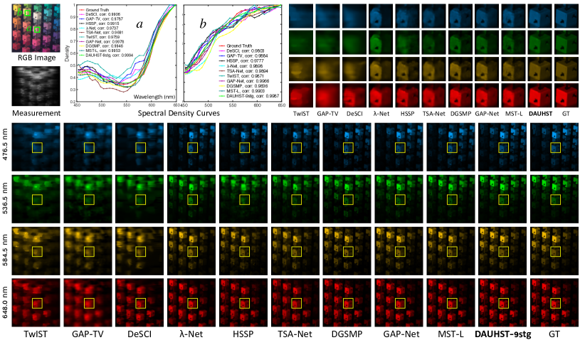
Figure 4: Simulation HSI reconstruction comparisons of Scene 2 with 4 (out of 28) spectral channels. The top-middle shows the spectral curves corresponding to the two green boxes of the RGB image. The top-right depicts the enlarged patches corresponding to the yellow boxes in the bottom HSIs. Zoom in for a better view.

3 Experiment

3.1 Experiment Setup

Similar to tsa_net ; hdnet ; gapnet ; gsm ; mst , 28 wavelengths are selected from 450nm to 650nm and derived by spectral interpolation manipulation for the HSI data. Simulation and real experiments are conducted.

Simulation Dataset. We adopt two datasets, i.e., CAVE cave and KAIST kaist for simulation experiments. The CAVE dataset consists of 32 HSIs with spatial size 512$\times$512. The KAIST dataset contains 30 HSIs of spatial size 2704$\times$3376. Following the settings of tsa_net ; hdnet ; gapnet ; gsm ; mst , the CAVE dataset is adopted as the training set while 10 scenes from the KAIST dataset are selected for testing.

Real Dataset. Five real HSIs collected by the CASSI system developed in tsa_net are used for testing.

Implementation Details. We implement DAUHST by Pytorch. All DAUHST models are trained with Adam adam optimizer ($\beta_{1}$ = 0.9 and $\beta_{2}$ = 0.999) using Cosine Annealing scheme cosine for 300 epochs on an RTX 3090 GPU. The initial learning rate is 4$\times$10^-4. Patches with spatial sizes 256$\times$256 and 660$\times$660 are randomly cropped from the 3D HSI cubes with 28 channels as training samples for the simulation and real experiments. The shifting step $d$ in the dispersion is set to 2. The batch size is 5. We set the basic channel $C$ = $N_{\lambda}$ = 28 to store HSI information. The weights of $\mathcal{D}$ in different stages are unshared. Data augmentation includes random rotation and flipping. The training objective is to minimize the Root Mean Square Error (RMSE) between reconstructed and ground-truth HSIs.

3.2 Quantitative Comparisons with State-of-the-Art Methods

Tab. 1 compares the results of DAUHST and 16 SOTA methods including three model-based methods (TwIST twist , GAP-TV gap_tv , and DeSCI desci ), one PnP method (DIP-HSI self ), seven E2E methods ($\lambda$-Net lambda , TSA-Net tsa_net , HDNet hdnet , MST mst , MST++ mst_pp , CST cst , and BIRNAT birnat ), and five deep unfolding methods (HSSP hssp , DNU dnu , DGSMP gsm , GAP-Net gapnet , and ADMM-Net admm-net ) on 10 simulation scenes. All algorithms are tested with the same settings as gsm ; mst .

(i) Our best model DAUHST-9stg (9-stage DAUHST) yields very impressive results, i.e., 38.36 dB in PSNR and 0.967 in SSIM. DAUHST-9stg significantly outperforms two recent SOTA methods BIRNAT birnat and MST-L mst by 0.78 and 3.18 dB, suggesting the effectiveness of our method.

(ii) Our DAUHST models dramatically surpass SOTA methods while requiring cheaper computational and memory costs. For instance, when compared with the only one Transformer-based E2E method MST, our DAUHST-2stg outperforms MST-L by 1.16 dB but only costs 68.9% (1.40 / 2.03) Params and 65.5% (18.44 / 28.15) FLOPS. When compared with CNN-based E2E methods, DAUHST-3stg surpasses HDNet, TSA-Net, and $\lambda$-Net by 2.24, 5.75, and 8.68 dB while only requiring 87.8%, 4.7%, 3.3% Params and 17.6%, 24.7%, 23.0% FLOPS. When compared with RNN-based E2E method BIRNAT, our DAUHST-5stg is 0.17 dB higher but only costs 2.1% FLOPS and 78.2% Params. Fig. 1 plots the PSNR-FLOPS comparisons of DAUHST and SOTA unfolding methods. DAUHST outperforms other competitors with the same number of stages by very large margins, over 4 dB.

3.3 Qualitative Comparisons with State-of-the-Art Methods

Simulation HSI Reconstruction. Fig. 4 depicts the simulation HSI reconstruction comparisons between our DAUHST and other SOTA methods on Scene 2 with 4 (out of 28) spectral channels. The top-right part shows the zoomed-in patches of the yellow boxes in the entire HSIs (bottom). As can be observed that our DAUHST-9stg is more favorable to reconstruct visually pleasant HSIs with more detailed contents, cleaner textures, and fewer artifacts while preserving the spatial smoothness of homogeneous regions. In contrast, previous methods either yield over-smooth results compromising fine-grained structures, or introduce undesired chromatic artifacts and blotchy textures that are absent in the ground truth (GT). The top-middle part illustrates the density-wavelength spectral curves corresponding to the green boxes identified as a and b in the RGB image (top-left). The spectral curves of DAUHST-9stg achieve the highest correlation and coincidence with the reference curves, showing the advantage of our proposed DAUHST in spectral-dimension consistency reconstruction.

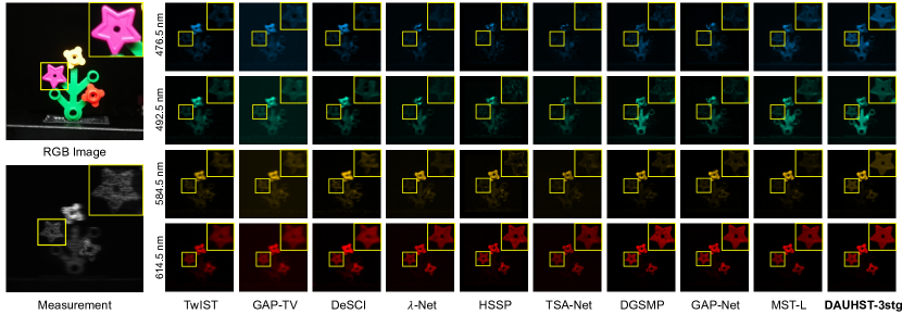
Figure 5: Real HSI reconstruction results of DAUHST-3stg and 9 SOTA methods on Scene 1 with 4 (out of 28) spectra. Only our method can clearly reconstruct the picked flower at all wavelengths. Zoom in for a better view.

Real HSI Reconstruction. We further evaluate the effectiveness of DAUHST in real HSI reconstruction. Following the same settings as tsa_net ; gsm ; mst for a fair comparison, we re-train DAUHST-3stg with the real mask on the CAVE and KAIST datasets jointly. To simulate the real imaging situations, the training samples are also injected with 11-bit shot noise. Fig. 5 shows the visual comparisons between our DAUHST-3stg and nine SOTA methods. In the top three rows, only our DAUHST-3stg can reconstruct the flower patch corresponding to the yellow box at all wavelengths while other methods all fail to recover the entire patch. In the bottom row, DAUHST-3stg restores more HSI structural details and clearer contents with fewer artifacts. In contrast, other methods recover blurry images, generate incomplete responses, and are susceptible to the noise corruption. This evidence suggests that DAUHST is more robust to the noise distortion and more effective in real HSI reconstruction.

3.4 Ablation Study

Break-down Ablation. We adopt baseline-1 that is derived by removing HS-MSA and DAUF from DAUHST-3stg to conduct the break-down ablation. Our goal is to study the effect of each component towards higher performance. Baseline-1 is cascaded end to end by three single-stage networks. As shown in Tab. 2a, baseline-1 achieves 33.05 dB. When we respectively apply DAUF and HS-MSA, the model achieves 2.32 and 2.44 dB improvements. When we exploit DAUF and HS-MSA jointly, the model gains by 4.16 dB. These results demonstrate the effectiveness of our DAUF and HS-MSA.

Self-Attention Mechanism. To compare HS-MSA with other MSAs, we adopt baseline-2 that is obtained by removing HS-MSA from DAUHST-1stg to conduct the ablation in Tab. 2b. We remove different position embedding schemes to avoid their impacts and only compare MSAs. For fairness, we keep the Params of MSAs the same by fixing the number of channels and heads. Baseline-2 yields 32.79 dB. We apply global MSA (G-MSA) global_msa , Swin MSA (SW-MSA) liu2021swin , Spectral-wise MSA (S-MSA) mst , and HS-MSA. Note that we downsample the input feature maps of G-MSA to avoid memory bottlenecks. As shown in Tab. 2b, HS-MSA yields the most significant improvement of 1.26 dB, which is 0.42, 0.30, and 0.23 dB higher than G-MSA, SW-MSA, and S-MSA. This superiority is mainly derived from HS-MSA’s ability to jointly capture local contents and non-local dependencies.

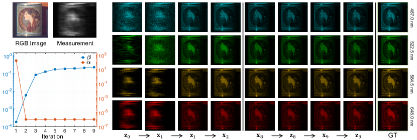
Figure 6: Visualization of $\mathbf{z}_{k}$ and $\mathbf{x}_{k}$ with 4 (out of 28) spectral channels on $Scene$ 1 in different iterations. The bottom-left corner plots the curves of $\boldsymbol{\alpha}$ and $\boldsymbol{\beta}$ changing with the iteration. Please zoom in for a better view.

Baseline-1	DAUF	HS-MSA	PSNR	SSIM	Params (M)	FLOPS (G)
✓			33.05	0.912	1.06	17.62
✓	✓		35.37	0.938	1.11	18.55
✓		✓	35.49	0.941	2.03	26.23
✓	✓	✓	37.21	0.959	2.08	27.17

(a) Break-down ablation towards higher performance.

Method	Baseline-2	G-MSA	SW-MSA	S-MSA	HS-MSA
PSNR	32.79	33.63	33.75	33.82	34.05
SSIM	0.904	0.920	0.924	0.926	0.930
Params (M)	0.40	0.48	0.48	0.48	0.48
FLOPS (G)	6.85	10.30	9.41	8.89	9.72

(b) Ablation of various self-attention mechanisms.

Framework	DNU dnu	ADMM admm-net	GAP gapnet	DAUF
PSNR	34.62	35.52	35.58	37.21
SSIM	0.930	0.942	0.943	0.959
Params (M)	2.03	2.03	2.03	2.08
FLOPS (G)	26.23	26.23	26.23	27.17

(c) Ablation of different unfolding frameworks.

Baseline-3	$\boldsymbol{\alpha}$	$\boldsymbol{\beta}$	PSNR	SSIM	Params (M)	FLOPS (G)
✓			36.49	0.952	2.03	26.23
✓	✓		36.94	0.957	2.08	27.10
✓		✓	36.83	0.956	2.08	27.17
✓	✓	✓	37.21	0.959	2.08	27.17

(d) Ablation to study the effect of parameters $\boldsymbol{\alpha}$ and $\boldsymbol{\beta}$.

Table 2: Ablation studies on simulation datasets cave ; kaist . PSNR, SSIM, Params, and FLOPS are reported.

Unfolding Framework. We compare our DAUF with previous unfolding frameworks including DNU dnu , ADMM-Net admm-net , and GAP-Net gapnet . For a fair comparison, we replace each single-stage network of DNU, ADMM-Net, and GAP-Net by our HST. 3-stage architecture is adopted to conduct ablations. The results are shown in Tab. 2c. Our DAUF significantly outperforms DNU, ADMM, and GAP by 2.59, 1.69, and 1.63 dB while adding only 0.05M Params and 0.94G FLOPS. This is mainly because DAUF uses the parameters estimated from the compressed measurement and physical mask in the CASSI system to direct the iterative learning. These parameters capture critical information of CASSI degradation patterns and ill-posedness degree, providing key cues for HSI reconstruction.

To study the effect of the estimated parameters $\boldsymbol{\alpha}$ and $\boldsymbol{\beta}$, we perform a break-down ablation of DAUF. We adopt DAUHST-3stg as baseline-3 but $\boldsymbol{\alpha}$ is set as learnable parameters instead of being estimated by $\mathcal{E}$ in Eq. (12) and $\boldsymbol{\beta}$ is not fed into $\mathcal{D}$. The results are shown in Tab. 2d. Baseline-3 yields 36.49 dB. When $\boldsymbol{\alpha}$ is set to be estimated by $\mathcal{E}$, baseline-3 is improved by 0.45 dB. When $\boldsymbol{\beta}$ is fed into $\mathcal{D}$, baseline-3 gains by 0.34 dB. When $\boldsymbol{\alpha}$ and $\boldsymbol{\beta}$ are exploited jointly in the iterative learning, baseline-3 achieves a significant improvement of 0.72 dB. These results verify that the estimated parameters $\boldsymbol{\alpha}$ and $\boldsymbol{\beta}$ are beneficial for the linear projection and denoising network of deep unfolding methods.

To further analyze the roles of the estimated parameters, we visualize $\mathbf{z}_{k}$ and $\mathbf{x}_{k}$ of Eq. (12), and plot the curves of $\boldsymbol{\alpha}$ and $\boldsymbol{\beta}$ as they change with the iteration in Fig. 6. We observe: (i) $\mathbf{z}_{0}$ and $\mathbf{x}_{1}$ yield either blurry or noisy images. There is a significant gap between them. Since $\alpha_{k}=\mu_{k}$ in Eq. (5) penalizes the differences between $\mathbf{z}$ and $\mathbf{x}$, $\alpha_{1}$ is estimated to be a large value. From the linear projection of the second iteration ($\mathbf{z}_{1}\rightarrow\mathbf{x}_{2}$) on, the gap between $\mathbf{z}$ and $\mathbf{x}$ decreases substantially. Therefore, $\alpha_{k}$ are estimated to be small values when $k\geq 2$. This indicates that $\boldsymbol{\alpha}$ can adaptively scale the linear projection $\mathcal{P}$. (ii) The noise corruption is severe in the first iteration. Thus, $\beta_{1}$ = $\mu_{1}/\tau_{1}$ = ${1/}{(\sqrt{\tau_{1}/\mu_{1}})^{2}}$, which is inversely proportional to the noise level, is estimated to be a small value. With further iterations, the noise level decreases, and thus the estimated $\beta_{k}$ increases. These results demonstrate that $\boldsymbol{\beta}$ can provide the information about noise level for the denoising network $\mathcal{D}$.

4 Conclusion

In this paper, we remedy two issues of previous deep unfolding methods, i.e., they do not estimate informative parameters from the CASSI system to direct the iterative learning and they are mainly CNN-based showing limitations in capturing long-range dependencies. To cope with these challenges, we firstly formulate a principled MAP-based unfolding framework DAUF that estimates parameters from the compressed measurement and physical mask. Then the parameters, which capture critical cues of CASSI degradation patterns and ill-posedness degree, are fed into each iteration to contextually scale the linear projection and provide noise level information for the denoising network. Secondly, we propose a novel Transformer HST that can jointly extract local contents and model non-local dependencies. By plugging HST into DAUF, we derive the first Transformer-based unfolding method DAUHST for HSI reconstruction. Comprehensive experiments show that our DAUHST outperforms SOTA methods by a large margin while requiring much cheaper memory and computational costs.

References

- (1) M. Fauvel, Y. Tarabalka, J. A. Benediktsson, J. Chanussot, and J. C. Tilton, “Advances in spectral-spatial classification of hyperspectral images,” Proceedings of the IEEE, 2012.
- (2) E. Maggiori, G. Charpiat, Y. Tarabalka, and P. Alliez, “Recurrent neural networks to correct satellite image classification maps,” Transactions on Geoscience and Remote Sensing, 2017.
- (3) F. Zhang, B. Du, and L. Zhang, “Scene classification via a gradient boosting random convolutional network framework,” Transactions on Geoscience and Remote Sensing, 2015.
- (4) M. H. Kim, T. A. Harvey, D. S. Kittle, H. Rushmeier, R. O. P. J. Dorsey, and D. J. Brady, “3d imaging spectroscopy for measuring hyperspectral patterns on solid objects,” ACM Transactions on on Graphics, 2012.
- (5) Z. Pan, G. Healey, M. Prasad, and B. Tromberg, “Face recognition in hyperspectral images,” TPAMI, 2003.
- (6) H. V. Nguyen, A. Banerjee, and R. Chellappa, “Tracking via object reflectance using a hyperspectral video camera,” in CVPRW, 2010.
- (7) Y. Fu, Y. Zheng, I. Sato, and Y. Sato, “Exploiting spectral-spatial correlation for coded hyperspectral image restoration,” in CVPR, 2016.
- (8) B. Uzkent, M. J. Hoffman, and A. Vodacek, “Real-time vehicle tracking in aerial video using hyperspectral features,” in CVPRW, 2016.
- (9) B. Uzkent, A. Rangnekar, and M. Hoffman, “Aerial vehicle tracking by adaptive fusion of hyperspectral likelihood maps,” in CVPRW, 2017.
- (10) V. Backman, M. B. Wallace, L. Perelman, J. Arendt, R. Gurjar, M. Muller, Q. Zhang, G. Zonios, E. Kline, and T. McGillican, “Detection of preinvasive cancer cells,” Nature, 2000.
- (11) G. Lu and B. Fei, “Medical hyperspectral imaging: a review,” Journal of Biomedical Optics, 2014.
- (12) Z. Meng, M. Qiao, J. Ma, Z. Yu, K. Xu, and X. Yuan, “Snapshot multispectral endomicroscopy,” Optics Letters, 2020.
- (13) M. Borengasser, W. S. Hungate, and R. Watkins, “Hyperspectral remote sensing: principles and applications,” CRC press, 2007.
- (14) F. Melgani and L. Bruzzone, “Classification of hyperspectral remote sensing images with support vector machines,” IEEE Transactions on Geoscience and Remote Sensing, 2004.
- (15) Y. Yuan, X. Zheng, and X. Lu, “Hyperspectral image superresolution by transfer learning,” IEEE Journal of Selected Topics in Applied Earth Observations and Remote Sensing, 2017.
- (16) J. Solomon and B. Rock, “Imaging spectrometry for earth remote sensing,” Science, 1985.
- (17) P. Llull, X. Liao, X. Yuan, J. Yang, D. Kittle, L. Carin, G. Sapiro, and D. J. Brady, “Coded aperture compressive temporal imaging,” Optics Express, 2013.
- (18) A. Wagadarikar, R. John, R. Willett, and D. Brady, “Single disperser design for coded aperture snapshot spectral imaging,” Applied Optics, 2008.
- (19) A. A. Wagadarikar, N. P. Pitsianis, X. Sun, and D. J. Brady, “Video rate spectral imaging using a coded aperture snapshot spectral imager,” Optics Express, 2009.
- (20) X. Cao, T. Yue, X. Lin, S. Lin, X. Yuan, Q. Dai, L. Carin, and D. J. Brady, “Computational snapshot multispectral cameras: Toward dynamic capture of the spectral world,” IEEE Signal Processing Magazine, 2016.
- (21) H. Du, X. Tong, X. Cao, and S. Lin, “A prism-based system for multispectral video acquisition,” in ICCV, 2009.
- (22) X. Yuan, T.-H. Tsai, R. Zhu, P. Llull, D. Brady, and L. Carin, “Compressive hyperspectral imaging with side information,” IEEE Journal of selected topics in Signal Processing, 2015.
- (23) X. Ma, X. Yuan, C. Fu, and G. R. Arce, “Led-based compressive spectral-temporal imaging,” Optics Express, 2021.
- (24) Z. Meng, J. Ma, and X. Yuan, “End-to-end low cost compressive spectral imaging with spatial-spectral self-attention,” in ECCV, 2020.
- (25) M. E. Gehm, R. John, D. J. Brady, R. M. Willett, and T. J. Schulz, “Single-shot compressive spectral imaging with a dual-disperser architecture,” Optics express, 2007.
- (26) D. Kittle, K. Choi, A. Wagadarikar, and D. J. Brady, “Multiframe image estimation for coded aperture snapshot spectral imagers,” Applied optics, 2010.
- (27) Y. Liu, X. Yuan, J. Suo, D. Brady, and Q. Dai, “Rank minimization for snapshot compressive imaging,” TPAMI, 2019.
- (28) L. Wang, Z. Xiong, G. Shi, F. Wu, and W. Zeng, “Adaptive nonlocal sparse representation for dual-camera compressive hyperspectral imaging,” TPAMI, 2016.
- (29) S. Zhang, L. Wang, Y. Fu, X. Zhong, and H. Huang, “Computational hyperspectral imaging based on dimension-discriminative low-rank tensor recovery,” in ICCV, 2019.
- (30) X. Yuan, “Generalized alternating projection based total variation minimization for compressive sensing,” in ICIP, 2016.
- (31) J. Tan, Y. Ma, H. Rueda, D. Baron, and G. R. Arce, “Compressive hyperspectral imaging via approximate message passing,” IEEE Journal of Selected Topics in Signal Processing, 2016.
- (32) M. A. Figueiredo, R. D. Nowak, and S. J. Wright, “Gradient projection for sparse reconstruction: Application to compressed sensing and other inverse problems,” IEEE Journal of selected topics in signal processing, 2007.
- (33) S. H. Chan, X. Wang, and O. A. Elgendy, “Plug-and-play admm for image restoration: Fixed-point convergence and applications,” Transactions on Computational Imaging, 2016.
- (34) M. Qiao, X. Liu, and X. Yuan, “Snapshot spatial–temporal compressive imaging,” Optics letters, 2020.
- (35) X. Yuan, Y. Liu, J. Suo, and Q. Dai, “Plug-and-play algorithms for large-scale snapshot compressive imaging,” in CVPR, 2020.
- (36) Z. Meng, Z. Yu, K. Xu, and X. Yuan, “Self-supervised neural networks for spectral snapshot compressive imaging,” in ICCV, 2021.
- (37) S. Zheng, Y. Liu, Z. Meng, M. Qiao, Z. Tong, X. Yang, S. Han, and X. Yuan, “Deep plug-and-play priors for spectral snapshot compressive imaging,” Photonics Research, 2021.
- (38) X. Yuan, Y. Liu, J. Suo, F. Durand, and Q. Dai, “Plug-and-play algorithms for video snapshot compressive imaging,” TPAMI, 2021.
- (39) M. Qiao, Z. Meng, J. Ma, and X. Yuan, “Deep learning for video compressive sensing,” Apl Photonics, 2020.
- (40) X. Hu, Y. Cai, J. Lin, H. Wang, X. Yuan, Y. Zhang, R. Timofte, and L. V. Gool, “Hdnet: High-resolution dual-domain learning for spectral compressive imaging,” in CVPR, 2022.
- (41) X. Miao, X. Yuan, Y. Pu, and V. Athitsos, “l-net: Reconstruct hyperspectral images from a snapshot measurement,” in ICCV, 2019.
- (42) X. Yuan, D. J. Brady, and A. K. Katsaggelos, “Snapshot compressive imaging: Theory, algorithms, and applications,” IEEE Signal Processing Magazine, 2021.
- (43) L. Wang, C. Sun, M. Zhang, Y. Fu, and H. Huang, “Dnu: Deep non-local unrolling for computational spectral imaging,” in CVPR, 2020.
- (44) L. Wang, C. Sun, Y. Fu, M. H. Kim, and H. Huang, “Hyperspectral image reconstruction using a deep spatial-spectral prior,” in CVPR, 2019.
- (45) Z. Meng, S. Jalali, and X. Yuan, “Gap-net for snapshot compressive imaging,” arXiv preprint arXiv:2012.08364, 2020.
- (46) J. Ma, X.-Y. Liu, Z. Shou, and X. Yuan, “Deep tensor admm-net for snapshot compressive imaging,” in ICCV, 2019.
- (47) T. Huang, W. Dong, X. Yuan, J. Wu, and G. Shi, “Deep gaussian scale mixture prior for spectral compressive imaging,” in CVPR, 2021.
- (48) Y. Fu, Z. Liang, and S. You, “Bidirectional 3d quasi-recurrent neural network for hyperspectral image super-resolution,” Journal of Selected Topics in Applied Earth Observations and Remote Sensing, 2021.
- (49) X. Zhang, Y. Zhang, R. Xiong, Q. Sun, and J. Zhang, “Herosnet: Hyperspectral explicable reconstruction and optimal sampling deep network for snapshot compressive imaging,” in CVPR, 2022.
- (50) A. Vaswani, N. Shazeer, N. Parmar, J. Uszkoreit, L. Jones, A. N. Gomez, Ł. Kaiser, and I. Polosukhin, “Attention is all you need,” in NeurIPS, 2017.
- (51) Z. Liu, Y. Lin, Y. Cao, H. Hu, Y. Wei, Z. Zhang, S. Lin, and B. Guo, “Swin transformer: Hierarchical vision transformer using shifted windows,” in ICCV, 2021.
- (52) A. Arnab, M. Dehghani, G. Heigold, C. Sun, M. Lučić, and C. Schmid, “Vivit: A video vision transformer,” arXiv preprint arXiv:2103.15691, 2021.
- (53) A. Dosovitskiy, L. Beyer, A. Kolesnikov, D. Weissenborn, X. Zhai, T. Unterthiner, M. Dehghani, M. Minderer, G. Heigold, S. Gelly, J. Uszkoreit, and N. Houlsby, “An image is worth 16x16 words: Transformers for image recognition at scale,” in ICLR, 2021.
- (54) S. Bhojanapalli, A. Chakrabarti, D. Glasner, D. Li, T. Unterthiner, and A. Veit, “Understanding robustness of transformers for image classification,” in ICCV, 2021.
- (55) P. Ramachandran, N. Parmar, A. Vaswani, I. Bello, A. Levskaya, and J. Shlens, “Stand-alone self-attention in vision models,” in NeurIPS, 2019.
- (56) A. El-Nouby, H. Touvron, M. Caron, P. Bojanowski, M. Douze, A. Joulin, I. Laptev, N. Neverova, G. Synnaeve, J. Verbeek, et al., “Xcit: Cross-covariance image transformers,” arXiv preprint arXiv:2106.09681, 2021.
- (57) C.-F. R. Chen, Q. Fan, and R. Panda, “Crossvit: Cross-attention multi-scale vision transformer for image classification,” in ICCV, 2021.
- (58) X. Zhu, W. Su, L. Lu, B. Li, X. Wang, and J. Dai, “Deformable detr: Deformable transformers for end-to-end object detection,” in ICLR, 2021.
- (59) Z. Yang, Y. Wei, and Y. Yang, “Associating objects with transformers for video object segmentation,” in NeurIPS, 2021.
- (60) N. Carion, F. Massa, G. Synnaeve, N. Usunier, A. Kirillov, and S. Zagoruyko, “End-to-end object detection with transformers,” in ECCV, 2020.
- (61) X. Dai, Y. Chen, J. Yang, P. Zhang, L. Yuan, and L. Zhang, “Dynamic detr: End-to-end object detection with dynamic attention,” in ICCV, 2021.
- (62) I. Misra, R. Girdhar, and A. Joulin, “An end-to-end transformer model for 3d object detection,” in ICCV, 2021.
- (63) Y. Fang, B. Liao, X. Wang, J. Fang, J. Qi, R. Wu, J. Niu, and W. Liu, “You only look at one sequence: Rethinking transformer in vision through object detection,” in NeurIPS, 2021.
- (64) S. Zheng, J. Lu, H. Zhao, X. Zhu, Z. Luo, Y. Wang, Y. Fu, J. Feng, T. Xiang, P. H. Torr, and L. Zhang, “Rethinking semantic segmentation from a sequence-to-sequence perspective with transformers,” in CVPR, 2021.
- (65) H. Cao, Y. Wang, J. Chen, D. Jiang, X. Zhang, Q. Tian, and M. Wang, “Swin-unet: Unet-like pure transformer for medical image segmentation,” arXiv preprint arXiv:2105.05537, 2021.
- (66) E. Xie, W. Wang, Z. Yu, A. Anandkumar, J. M. Alvarez, and P. Luo, “Segformer: Simple and efficient design for semantic segmentation with transformers,” in NeurIPS, 2021.
- (67) R. Strudel, R. Garcia, I. Laptev, and C. Schmid, “Segmenter: Transformer for semantic segmentation,” in ICCV, 2021.
- (68) Z. Lu, S. He, X. Zhu, L. Zhang, Y.-Z. Song, and T. Xiang, “Simpler is better: Few-shot semantic segmentation with classifier weight transformer,” in ICCV, 2021.
- (69) Y. Li, S. Zhang, Z. Wang, S. Yang, W. Yang, S.-T. Xia, and E. Zhou, “Tokenpose: Learning keypoint tokens for human pose estimation,” in ICCV, 2021.
- (70) S. Yang, Z. Quan, M. Nie, and W. Yang, “Transpose: Keypoint localization via transformer,” in ICCV, 2021.
- (71) Y. Cai, Z. Wang, Z. Luo, B. Yin, A. Du, H. Wang, X. Zhou, E. Zhou, X. Zhang, and J. Sun, “Learning delicate local representations for multi-person pose estimation,” in ECCV, 2020.
- (72) K. Li, S. Wang, X. Zhang, Y. Xu, W. Xu, and Z. Tu, “Pose recognition with cascade transformers,” in CVPR, 2021.
- (73) C. Zheng, S. Zhu, M. Mendieta, T. Yang, C. Chen, and Z. Ding, “3d human pose estimation with spatial and temporal transformers,” in ICCV, 2021.
- (74) Y. Li, M. Hao, Z. Di, N. B. Gundavarapu, and X. Wang, “Test-time personalization with a transformer for human pose estimation,” in NeurIPS, 2021.
- (75) W. Mao, Y. Ge, C. Shen, Z. Tian, X. Wang, and Z. Wang, “Tfpose: Direct human pose estimation with transformers,” arXiv preprint arXiv:2103.15320, 2021.
- (76) H. Chen, Y. Wang, T. Guo, C. Xu, Y. Deng, Z. Liu, S. Ma, C. Xu, C. Xu, and W. Gao, “Pre-trained image processing transformer,” in CVPR, 2021.
- (77) J. Liang, J. Cao, G. Sun, K. Zhang, L. Van Gool, and R. Timofte, “Swinir: Image restoration using swin transformer,” in ICCVW, 2021.
- (78) Z. Wang, X. Cun, J. Bao, W. Zhou, J. Liu, and H. Li, “Uformer: A general u-shaped transformer for image restoration,” in CVPR, 2022.
- (79) J. Cao, Y. Li, K. Zhang, and L. Van Gool, “Video super-resolution transformer,” arXiv preprint arXiv:2106.06847, 2021.
- (80) J. Lin, Y. Cai, X. Hu, H. Wang, Y. Yan, X. Zou, H. Ding, Y. Zhang, R. Timofte, and L. Van Gool, “Flow-guided sparse transformer for video deblurring,” arXiv preprint arXiv:2201.01893, 2022.
- (81) Y. Cai, J. Lin, X. Hu, H. Wang, X. Yuan, Y. Zhang, R. Timofte, and L. V. Gool, “Mask-guided spectral-wise transformer for efficient hyperspectral image reconstruction,” in CVPR, 2022.
- (82) Y. Cai, J. Lin, Z. Lin, H. Wang, Y. Zhang, H. Pfister, R. Timofte, and L. V. Gool, “Mst++: Multi-stage spectral-wise transformer for efficient spectral reconstruction,” in CVPRW, 2022.
- (83) J. Lin, Y. Cai, X. Hu, H. Wang, X. Yuan, Y. Zhang, R. Timofte, and L. Van Gool, “Coarse-to-fine sparse transformer for hyperspectral image reconstruction,” arXiv preprint arXiv:2203.04845, 2022.
- (84) Y. Cai, X. Hu, H. Wang, Y. Zhang, H. Pfister, and D. Wei, “Learning to generate realistic noisy images via pixel-level noise-aware adversarial training,” in NeurIPS, 2021.
- (85) Z. Deng, Y. Cai, L. Chen, Z. Gong, Q. Bao, X. Yao, D. Fang, S. Zhang, and L. Ma, “Rformer: Transformer-based generative adversarial network for real fundus image restoration on a new clinical benchmark,” arXiv preprint arXiv:2201.00466, 2022.
- (86) J. A. Tropp and A. C. Gilbert, “Signal recovery from random measurements via orthogonal matching pursuit,” IEEE Transactions on Information Theory, 2007.
- (87) D. L. Donoho, “Compressed sensing,” IEEE Transactions on Information Theory, 2006.
- (88) S. Jalali and X. Yuan, “Snapshot compressed sensing: Performance bounds and algorithms,” Transactions on Information Theory, 2019.
- (89) X. Zhang, X. Zhou, M. Lin, and J. Sun, “Shufflenet: An extremely efficient convolutional neural network for mobile devices,” in CVPR, 2018.
- (90) J. Bioucas-Dias and M. Figueiredo., “A new twist: Two-step iterative shrinkage/thresholding algorithms for image restoration.,” TIP, 2007.
- (91) Z. Cheng, B. Chen, R. Lu, Z. Wang, H. Zhang, Z. Meng, and X. Yuan, “Recurrent neural networks for snapshot compressive imaging,” TPAMI, 2022.
- (92) J.-I. Park, M.-H. Lee, M. D. Grossberg, and S. K. Nayar, “Multispectral imaging using multiplexed illumination,” in ICCV, 2007.
- (93) I. Choi, M. Kim, D. Gutierrez, D. Jeon, and G. Nam, “High-quality hyperspectral reconstruction using a spectral prior,” in Technical report, 2017.
- (94) D. P. Kingma and J. L. Ba, “Adam: A method for stochastic optimization,” in ICLR, 2015.
- (95) I. Loshchilov and F. Hutter, “Sgdr: Stochastic gradient descent with warm restarts,” in ICLR, 2017.