Adversarial joint attacks on legged robots

Abstract

We address adversarial attacks on the actuators at the joints of legged robots trained by deep reinforcement learning. The vulnerability to the joint attacks can significantly impact the safety and robustness of legged robots. In this study, we demonstrate that the adversarial perturbations to the torque control signals of the actuators can significantly reduce the rewards and cause walking instability in robots. To find the adversarial torque perturbations, we develop black-box adversarial attacks, where, the adversary cannot access the neural networks trained by deep reinforcement learning. The black box attack can be applied to legged robots regardless of the architecture and algorithms of deep reinforcement learning. We employ three search methods for the black-box adversarial attacks: random search, differential evolution, and numerical gradient descent methods. In experiments with the quadruped robot Ant-v2 and the bipedal robot Humanoid-v2, in OpenAI Gym environments, we find that differential evolution can efficiently find the strongest torque perturbations among the three methods. In addition, we realize that the quadruped robot Ant-v2 is vulnerable to the adversarial perturbations, whereas the bipedal robot Humanoid-v2 is robust to the perturbations. Consequently, the joint attacks can be used for proactive diagnosis of robot walking instability.

I Introduction

With the recent progress in deep reinforcement learning for robot control, safety and robustness have become the primary concern. This concern is especially true for legged robots because they are prone to falling [1]. Many disturbances can affect the safety and robustness of legged robots. Among disturbances, one should pay attention to adversarial attacks [2, 3] because these attacks can significantly impact the safety and robustness with small perturbations. For legged robots, finding vulnerability to adversarial attacks leads to proactive detection of potential risks of falling.

This study deals with the adversarial attacks on the control of legged robots in deep reinforcement learning. In particular, we demonstrate that perturbations to the torque control signals of actuators at joints, which are essential components for walking, cause instability in walking motion. We use an adversarial attack [2, 3] to search such adversarial perturbations. Adversarial attacks in supervised learning seek input perturbations that reduce the loss for deep reinforcement learning, whereas, in this study, we seek torque perturbations that reduce the reward. The torque perturbations are possibly caused by the actuator’s modeling error, noise, or physical failure [4], rather than intentional attacks by the malicious adversary. Thus, finding vulnerability to the torque perturbations can be used to proactively diagnose robot-walking instability.

Many adversarial attacks in deep reinforcement learning perturb the state observations to cause the agents to malfunction [5, 6]. The attacks on the state observations allow white-box attacks where the adversary can access the neural networks, such as policy networks and Q-networks, that take the state observations as the input [7, 8, 9]. Conversely, we consider a black-box attack on the joint actuators of legged robots by perturbing the torque signals. This attack is defined in the action space. The adversarial attacks on the action space are usually black-box ones because the environment functions are neither neural networks nor differentiable functions, though white-box attacks are possible using proxy reward functions [10]. For legged robots, the environment functions are physical simulators or real-world trials. In addition, the black box attack can be applied to robots regardless of the architectures and algorithms of deep reinforcement learning.

Figure 1: Overall view of adversarial joint attack

We introduce three search methods for black-box adversarial joint attacks to legged robots: random search, differential evolution [11], and numerical gradient descent methods. These three methods generate torque perturbations that reduce the rewards by repeating walking simulations of legged robots. The torque perturbations are assumed to be fixed over time. We conduct experiments in the quadruped robot Ant-v2 and the bipedal robot Humanoid-v2 environments from OpenAI Gym[12]. These environments run on the physical engine MuJoCo [13]. We evaluate the effectiveness of the three search methods in terms of the average cumulative rewards. The experimental results reveal that the differential evolution method can efficiently detect the strongest torque perturbations among the three methods. In addition, we discover that the quadruped robot Ant-v2 is vulnerable to the adversarial perturbations, whereas the bipedal robot Humanoid-v2 is robust to the perturbations.

The key contributions of this study can be summarized as follows:

• We propose a black-box adversarial joint attack on legged robots.

• We demonstrate that the differential evolution method can efficiently find the strongest torque perturbations among the three methods.

• We discover the torque perturbations that interfere with the walking task for the first time.

Figure 2: Legged robot: Left Ant-v2, Right Humanoid-v2

II RELATED WORK

Adversarial attacks [3] on image classification in supervised learning apply small perturbations $\boldsymbol{\delta}_{x}$ to the input image $\boldsymbol{x}$ to misclassify the deep model. Such perturbations $\boldsymbol{\delta}_{x}$ are sought to maximize the loss function.

$$\operatorname*{\text{maxmize}}_{\boldsymbol{\delta}_{x}}J(\boldsymbol{x}+\boldsymbol{\delta}_{x}),\ \text{subject to}\ ||\boldsymbol{\delta}_{x}||_{p}\leq\epsilon,$$ (1)

where, $J(\cdot)$ is the loss function and $||\cdot||_{p}$ is the $p$-norm. For deep models, it is challenging to find the optimal solution of Eq. (1). As an approximate solution method, the gradient ascent method using the gradient of the loss function $\nabla_{\boldsymbol{x}}J(\boldsymbol{x})$ with respect to the input image $\boldsymbol{x}$ is used [3, 14]. To calculate the gradient $\nabla_{\boldsymbol{x}}J(\boldsymbol{x})$, the structure and parameters of the deep model are assumed to be known, and such an attack is called a white box attack.

Adversarial attacks on deep reinforcement learning are often formulated to minimize the expected reward. Because there are multiple attack targets (such as states, actions, environments, and rewards) various attacks are possible in deep reinforcement learning [6]. A well-known adversarial attack on TV gameplay [7] is defined on the state space, which attacks adds an adversarial perturbation $\boldsymbol{\delta_{x}}$ to the input TV screen $\boldsymbol{x}$. This attack is formulated the same as the optimization problem in Eq. (1) because the input is an image and the output action is discrete. There are several adversarial attacks against robot control with continuous states and actions such as those proposed in this study. One approach is to introduce an enemy agent that attacks the legged robot, and the two play against each other to obtain robust policies [15, 16, 17]. These methods attack the legged robot from the outside. Unlike those in this study, they do not assume any failures or modeling errors in the legged robot itself. For attacks in action space, similar to those in this study, Lee et al. [10] conducted a white-box attack on the proxy reward function to find adversarial perturbations that vary in space and time. Conversely, we assume physical failures and modeling errors and seek black-box time-fixed adversarial perturbations. Yang et. al [18] used the greedy method to search for adversarial failures, assuming failures that cause joints to stop moving altogether while acquiring robust measures by training on such failures. In this study, we do not consider binary expressions of the presence or absence of a fault but small torque perturbations.

III Simulation-based Adversarial Joint Attack

We introduce three adversarial attack methods for finding joint torque perturbations that can interfere with the walking movements of legged robots. First, we describe adversarial attacks on the action space and define joint torque perturbations. Next, we describe a simulation-based search to find the adversarial perturbation.

III-A Adversarial attacks on joints

In this study, we attack the legged robots by perturbing the action vector $\boldsymbol{a}_{t}\in\mathcal{R}^{N_{a}}$, which is stochastically generated by a policy network $\pi(\boldsymbol{a}_{t}|\boldsymbol{s}_{t})$ with a continuous state vector $\boldsymbol{s}_{t}\in\mathcal{R}^{N_{s}}$. The action vector $\boldsymbol{a}_{t}$ is the torque control signal of the joint actuators at time $t$, where, $\mathcal{R}$ is the real number set, and $N_{a}$ is the total number of the joint actuators. We denote the adversarial perturbation to the action vector $\boldsymbol{a}_{t}$ by $\boldsymbol{\delta}$. We assume that the perturbation $\boldsymbol{\delta}$ is fixed over time and it is multiplicative, i.e., the attacked action vector $\boldsymbol{a}^{\prime}_{t}$ is given by

$$\boldsymbol{a}^{\prime}_{t}=\boldsymbol{a}_{t}+\boldsymbol{\delta}\odot\boldsymbol{a}_{t},\ \text{where}\ ||\boldsymbol{\delta}||_{\infty}\leq\epsilon,$$ (2)

where, $\odot$ is the Hadamard product, which is the product of each component of the vectors. For the $i$-th torque control signal $a_{i,t}$ of $\boldsymbol{a}_{t}$, the signal is perturbed by

$$a^{\prime}_{i,t}=a_{i,t}+\delta_{i}a_{i,t}=(1+\delta_{i})a_{i,t}.$$ (3)

The time-fixed perturbation is possibly caused by either the actuator’s modeling error or physical failure, which both remain nearly fixed over time.

We seek the adversarial torque perturbations $\boldsymbol{\delta}$ by minimizing the expected cumulative reward as

$$\operatorname*{\text{minimize}}_{\boldsymbol{\delta}}\ E[C(\boldsymbol{\delta})],\ \text{subject to}\ ||\boldsymbol{\delta}||_{\infty}\leq\epsilon,$$ (4)

where, $C(\boldsymbol{\delta})$ is the cumulative reward attacked by the adversarial perturbation $\boldsymbol{\delta}$ and is defined as

$$C(\boldsymbol{\delta})=\sum_{t=0}^{T-1}R(\boldsymbol{s_{t}},\boldsymbol{a}_{t}+\boldsymbol{\delta}\odot\boldsymbol{a}_{t}),$$ (5)

where, $R(\boldsymbol{s_{t}},\boldsymbol{a}_{t})$ is the reward at time $t$ given state $\boldsymbol{s_{t}}$ and action $\boldsymbol{a}_{t}$. The expected value in Eq. (4) is taken with respect to a trajectory of states and actions $\{\boldsymbol{s}_{0},\boldsymbol{a}_{0},\boldsymbol{s}_{1},\boldsymbol{a}_{1},\ldots,\boldsymbol{s}_{T-1},\boldsymbol{a}_{T-1}\}$.

III-B Simulation-based Black-Box Search

We consider the black-box adversarial attack, where, we cannot access the policy network $\pi(\boldsymbol{a}_{t}|\boldsymbol{s}_{t})$ and we can only access the rewards $R(\boldsymbol{s_{t}},\boldsymbol{a}_{t})$ through the waling simulator. In this case, it is difficult to compute the gradient $\nabla_{\boldsymbol{a}}C(\boldsymbol{\delta})$ of the cumulative reward in Eq. (4) with respect to the action vector $\boldsymbol{a}$. Therefore, it is necessary to search for the adversarial perturbations by repeating walking simulations, that is, we empirically estimate the expected cumulative reward $E[C(\boldsymbol{\delta})]$ in Eq. (4) by taking the average of $M$ cumulative rewards as

$$E[C(\boldsymbol{\delta})]\approx\bar{C}(\boldsymbol{\delta})=\frac{1}{M}\sum_{m=1}^{M}C^{(m)}(\boldsymbol{\delta}),$$ (6)

where, $C^{(m)}(\boldsymbol{\delta})$ is a cumulative reward of the $m$-th walking simulation. For each simulation run, the initial state $\boldsymbol{s}_{0}$ is reset before the simulation. In the experiments, we set $M=100$. We employ three simulation-based search methods that minimize the empirical estimation in Eq. (6): random search, differential evolution, and numerical gradient descent methods.

III-B1 Random Search

We represent the random search method as Algorithm 1. The random search method randomly generates a set of torque perturbations $\boldsymbol{\delta}^{(n)},n=1,2,\ldots$. Each element of $\boldsymbol{\delta}^{(n)}$ is generated according to the uniform distribution $U([-\epsilon,\epsilon])$. For each perturbation $\boldsymbol{\delta}^{(n)}$, we run $M$ walking simulations and compute the average cumulative reward using Eq. (6). Then, we choose the best perturbation $\boldsymbol{\delta}_{\mathrm{best}}$ that minimizes the average cumulative reward as the adversarial perturbation.

Algorithm 1 Random Search for an Adversarial Attack

1:  $C_{\mathrm{min}}\leftarrow\infty$

2:  for each perturbation $n=1,2,\ldots$  do

3:     Generate torque perturbation $\boldsymbol{\delta}^{(n)}\sim U\left([-\epsilon,\epsilon]^{N_{a}}\right)$

4:     Compute average cumulative reward $\bar{C}(\boldsymbol{\delta}^{(n)})$​ in Eq.​ (6)

5:     if $\bar{C}(\boldsymbol{\delta}^{(n)})<C_{\mathrm{min}}$ then

6:        $C_{\mathrm{min}}\leftarrow\bar{C}(\boldsymbol{\delta}^{(n)})$

7:        Update best torque perturbation $\boldsymbol{\delta}_{\mathrm{best}}\leftarrow\boldsymbol{\delta}^{(n)}$

8:     end if

9:  end for

III-B2 Differential Evolution

We represent the differential evolution method as Algorithm 2. For differential evolution, we have a population of torque perturbations $\{\boldsymbol{\delta}_{g}^{(1)},\ldots,\boldsymbol{\delta}_{g}^{(NP)}\}$, where, $NP$ is the population size and the subscript $g$ stands for the $g$-th generation. Each element of the initial individual $\boldsymbol{\delta}_{0}^{(i)}$ is generated according to the uniform distribution $U\left([-\epsilon,\epsilon]\right)$. We use the average cumulative reward in Eq. (6) to evaluate the fitness of each individual $\boldsymbol{\delta}_{g}^{(i)}$. The best individual $\boldsymbol{\delta}_{\mathrm{best}}$ is one that yields the lowest average cumulative reward, not the highest.

We use the mutation and crossover processes for differential evolution as follows: For mutation, we choose the best/1 strategy and obtain the $i$-th mutant individual $\boldsymbol{v}_{g+1}^{(i)}$ as

$$\boldsymbol{v}_{g+1}^{(i)}=\boldsymbol{\delta}_{\mathrm{best}}+F(\boldsymbol{\delta}_{g}^{(r_{1})}-\boldsymbol{\delta}_{g}^{(r_{2})}),$$ (7)

where, $F\in(0.5,1]$ is a random coefficient, $r_{1}$ and $r_{2}$ are mutually exclusive indices randomly chosen from $\{1,2,\ldots,NP\}$. For crossover, we use the binomial crossover and obtain the $j$-th element of the $i$-th trial individual $\boldsymbol{u}_{g+1}^{(i)}$ as

$${u}_{j,g+1}^{(i)}=\left\{\begin{array}[]{ll}{v}_{j,g+1}^{(i)}&\text{if}\quad r\leq CR\ \text{or}\ j=j_{r}\\ {\delta}_{j,g}^{(i)}&\text{otherwise}\end{array}\right.$$ (8)

where, $r$ is a uniform random number in $[0,1]$, $CR=0.7$ is a crossover constant, and $j_{r}$ is an index randomly chosen from $[1,2,\ldots,N_{a}]$. We use the clip function to keep the perturbation within the range $[-\epsilon,\epsilon]$ element-wise. The clip function is defined by $\mathrm{clip}_{[-\epsilon,\epsilon]}(\boldsymbol{x})=\max(\min(\boldsymbol{x},\epsilon),-\epsilon)$, where, $\max$ and $\min$ are taken element-wise. Finally we choose the best individual $\boldsymbol{\delta}_{\mathrm{best}}$ from all generation populations.

Algorithm 2 Differential Evolution for an Adversarial Attack

0:  Population size $NP$

1:  Generate initial population of torque perturbations $\{\boldsymbol{\delta}_{0}^{(1)},\ldots,\boldsymbol{\delta}_{0}^{(NP)}\}$ with $\boldsymbol{\delta}_{0}^{(i)}\sim U\left([-\epsilon,\epsilon]^{N_{a}}\right)$

2:  $C_{\mathrm{min}}\leftarrow\infty$

3:  for each generation $g=1,2,\ldots$ do

4:     for each individual $i=1,2,\ldots,NP$ do

5:        Generate trial individual $\boldsymbol{u}_{g}^{(i)}$ by mutation and crossover in Eqs. (7) and (8)

6:        $\boldsymbol{u}_{g}^{(i)}\leftarrow\mathrm{clip}_{[-\epsilon,\epsilon]}(\boldsymbol{u}_{g}^{(i)})$

7:        Compute average cumulative rewards in Eq. (6) fortrial $\bar{C}_{(}\boldsymbol{u}_{g}^{(i)})$ and target $\bar{C}(\boldsymbol{\delta}_{g-1}^{(i)})$

8:        if $\bar{C}(\boldsymbol{u}_{g}^{(i)})\leq\bar{C}(\boldsymbol{\delta}_{g-1}^{(i)})$ then

9:           Accept trial individual $\boldsymbol{\delta}_{g}^{(i)}\leftarrow\boldsymbol{u}_{g}^{(i)}$

10:           if $\bar{C}(\boldsymbol{u}_{g}^{(i)})<C_{\mathrm{min}}$ then

11:              $C_{\mathrm{min}}\leftarrow\bar{C}(\boldsymbol{u}_{g}^{(i)})$

12:              Update best individual $\boldsymbol{\delta}_{\mathrm{best}}\leftarrow\boldsymbol{\delta}_{g}^{(i)}$

13:           end if

14:        else

15:           Retain target individual $\boldsymbol{\delta}_{g}^{(i)}\leftarrow\boldsymbol{\delta}_{g-1}^{(i)}$

16:        end if

17:     end for

18:  end for

III-B3 Numerical Gradient Descent

As mentioned previously, it is difficult to compute the gradient vector $\boldsymbol{g}=\nabla_{\boldsymbol{a}}C(\boldsymbol{\delta})$ of the cumulative reward for gradient descent. Therefore, we numerically approximate the gradient vector $\boldsymbol{g}$ using a finite difference method, that is, the $i$-th element of $\boldsymbol{g}$ is approximated by

$$g_{i}=\frac{\partial C(\boldsymbol{\delta})}{\partial a_{i}}\approx\frac{C(\boldsymbol{\delta}+\boldsymbol{h}_{i})-C(\boldsymbol{\delta})}{h},$$ (9)

where, $h$ is a finite difference and $\boldsymbol{h}_{i}$ is defined as a vector whose $i$-th element is $h$ and the rest are zeros, i.e., $\boldsymbol{h}_{i}=(0,\ldots,h,\ldots,0)$. $g_{i}$ is the gradient with respect to the torque signal of $i$-th actuator.

We represent the numerical gradient descent method as Algorithm 3. This algorithm terminates at a predetermined search time. In the algorithm, we use the clip function to keep the perturbation $\boldsymbol{\delta}$ within the range $[-\epsilon,\epsilon]$ element-wise.

Algorithm 3 Gradient Descent for an Adversarial Attack

1:  Initialize torque perturbation $\boldsymbol{\delta}\leftarrow(0,0,\ldots,0)$

2:  $C_{\mathrm{min}}\leftarrow\infty$

3:  while termination criterion is not met do

4:     Compute average cumulative reward $\bar{C}(\boldsymbol{\delta})$​ in Eq.​ (6)

5:     if $\bar{C}(\boldsymbol{\delta})<C_{\mathrm{min}}$ then

6:        $C_{\mathrm{min}}\leftarrow\bar{C}(\boldsymbol{\delta})$

7:        Update best torque perturbation $\boldsymbol{\delta}_{\mathrm{best}}\leftarrow\boldsymbol{\delta}$

8:     end if

9:     for each actuator $i=1,2,\ldots,N_{a}$ do

10:        Compute gradient $g_{i}$ in Eq. (9)

11:     end for

12:     Normalize gradient $\boldsymbol{g}\leftarrow\boldsymbol{g}/||\boldsymbol{g}||_{\infty}$

13:     $\boldsymbol{\delta}\leftarrow\mathrm{clip}_{[-\epsilon,\epsilon]}(\boldsymbol{\delta}-\alpha\boldsymbol{g})$

14:  end while

IV EXPERIMENTS with legged robots

This experiment aims to search for small perturbations to leg joints of legged robots, which interfere with the walking movements, and consequently find the most vulnerable joint. To this end, we compare the three search methods in terms of search capability and attack strength.

IV-A Experiment setup

We conduct experiments in the quadruped robot Ant-v2 and the bipedal robot Humanoid-v2 environ- ments from OpenAI Gym, as illustrated in Fig. 2. Ant-v2 and Humanoid-v2 have eight and seventeen joints, respectively. The simulation environment is built using the MuJoCo physics engine [13]. The task is forward walking, and the legged robot is trained to walk sufficiently using proximal policy optimization (PPO)[19] in advance.

The reward function for Ant-v2 is defined by

$$R(\boldsymbol{s},\boldsymbol{a})=v_{\text{fwd}}-0.5\|\boldsymbol{a}\|^{2}-0.5\cdot 10^{-3}\left\|\boldsymbol{f}\right\|^{2}+1,$$ (10)

and for Humanoid-v2 by

$$R(\boldsymbol{s},\boldsymbol{a})=3v_{\text{fwd}}-0.1\|\boldsymbol{a}\|^{2}-0.5\cdot 10^{-6}\left\|\boldsymbol{f}\right\|^{2}+5,$$ (11)

where, $v_{\text{fwd}}$ is the forward velocity, $\boldsymbol{a}$ is the torque signal vector, and $\boldsymbol{f}$ is the impact forces [20].

IV-B Comparison of search capability

Fig. 3 and 4 illustrate the average cumulative rewards $\bar{C}(\boldsymbol{\delta})$ of the best perturbation $\boldsymbol{\delta}_{\mathrm{best}}$ for random search (purple line), differential evolution (green line), and gradient descent (cyan line). For a fair comparison, the search time is set to 1250 min for Ant-v2 and 2250 min for Humanoid-v2. We plot the average cumulative rewards every five min in Figs. 3 and 4.

From Fig. 3, the differential evolution method (green line) can find the strongest attack parameters than the other two methods for Ant-v2. In addition, the differential evolution method stably converges and, it has the highest convergence speed. Conversely, Fig. 4 demonstrate that the differential method are comparable to the random search for Humanoid-v2. As mentioned below, Humanoid-v2 is robust to the adversarial attack. Therefore, the search methods cannot find effective perturbations.

Figure 3: Average cumulative rewards by three search methods (Ant-v2)

Figure 4: Average cumulative rewards by three search methods (Humanoid-v2)

IV-C Adversarial attack by differential evolution

As reported above, the differential evolution method can find the best adversarial perturbation among the three methods. This subsection evaluates the adversarial attacks by the differential evolution method. In experiments, we set the number of individuals to $NP=120$ for Ant-v2 and $NP=255$ for Humanoid-v2.

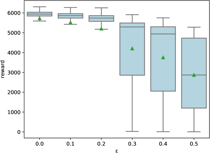
Figure 5: Cumulative reward distribution by differential evolution with varying attack strength $\epsilon$ (Ant-v2)

Figure 6: Cumulative reward distribution by differential evolution with varying attack strength $\epsilon$ (Humanoid-v2)

We test how the cumulative rewards are affected by the varying attack strength $\epsilon=0.0,0.1,0.2,0.3,0.4,0.5$. $\epsilon=0.0$ means no attack. Figs. 5 and 6 illustrate the box plots of the cumulative rewards by 1000 simulations. The green triangles in the plots are the average cumulative rewards. From Fig. 5, we observe that the attacks to Ant-v2 with $\epsilon=0.3$ and greater significantly reduce the cumulative rewards. These results indicate that Ant-v2 is vulnerable to the adversarial attacks. Conversely, from Fig. 6, we observe that the attacks on Humanoid-v2 do not change the cumulative rewards regardless of the attack strengths. Therefore we conclude that Humanoid-v2 is robust to the adversarial attacks. Unlike Ant-v2, which can stably walk with four legs, Humanoid-v2 has experienced many falls during learning and has learned how not to fall, thereby Humanoid-v2 became robust. Another possible explanation is that, the effect of the joint torques is not easily transmitted to walking because the feet in contact with the ground are fewer than in the case of Ant-v2.

((a)) Attack strength distributions per actuator

((b)) Most attacked actuators

Figure 7: Adversarial attacks on Ant-v2 for last generation individuals of differential evolution

TABLE I: Adversarial best torque perturbation for Ant-v2 ($\epsilon=0.5$)

body part	perturbation $\delta$
hip1	-0.01
ankle1	+0.09
hip2	+0.44
ankle2	+0.35
hip3	+0.33
ankle3	+0.45
hip4	+0.49
ankle4	+0.47

We further investigate the attacks on Ant-v2 using the strongest attack strength $\epsilon=0.5$. Table I shows the best perturbation $\boldsymbol{\delta}_{\mathrm{best}}$ by the differential evolution method with $\epsilon=0.5$. From the table, we observe that the attack strongly perturbs the three legs (hip2, ankle2, hip3, ankle3, hip4, and ankle4), and does not do the other leg (hip1 and ankle1). Thus, the attack unbalances the walking motion. Fig. 7 illustrates the histograms of the attack strengths of 120 individuals at the last generation for each actuator of Ant-v2. From Fig. 7, we observe that the individuals mostly attack the actuators at hip4 and ankle4 of Ant-v2, as illustrated in Fig. 7. Observing the walking simulation animation, as shown in the Fig. 8 (bottom), we find that these actuators are located at the primary leg for walking. The attacks on these actuators increase the magnitude of the torque signals and add an excessive vertical force. Consequently, Ant-v2 tends to fall as shown in the Fig. 8.

((a))

((b))

Figure 8: Illustration of quadruped robot locomotion for Ant-v2

V CONCLUSION

This study investigates the vulnerability to the adversarial joint attacks on the quadruped and bipedal robots trained by deep reinforcement learning. Deep reinforcement learning has been becoming popular for complex multi-degree-of-freedom control such as legged-robots control. Thus, it will increasingly become important to diagnose the vulnerability, safety, and robustness for real-world applications. This study demonstrates that the legged robot can be vulnerable to joint attacks and can be forced to fall.

In the experiments, we observed that differential evolution can efficiently find the strongest torque perturbations. Interestingly, the quadruped robot Ant-v2 is vulnerable and the bipedal robot Humanoid-v2 is robust. For future work, we will develop defense methods against adversarial joint attacks to improve the safety and robustness of legged robots.

References

- [1] Zhongyu Li, Xuxin Cheng, Xue Bin Peng, Pieter Abbeel, Sergey Levine, Glen Berseth, and Koushil Sreenath. Reinforcement learning for robust parameterized locomotion control of bipedal robots. In 2021 IEEE International Conference on Robotics and Automation (ICRA), pages 2811–2817, 2021.
- [2] Christian Szegedy, Wojciech Zaremba, Ilya Sutskever, Joan Bruna, Dumitru Erhan, Ian J. Goodfellow, and Rob Fergus. Intriguing properties of neural networks. In International Conference on Learning Representations., 2014.
- [3] Ian J. Goodfellow, Jonathon Shlens, and Christian Szegedy. Explaining and harnessing adversarial examples. In International Conference on Learning Rrepresentation, 2015.
- [4] Wataru Okamoto and Kazuhiko Kawamoto. Reinforcement learning with randomized physical parameters for fault-tolerant robots. In 2020 Joint 11th International Conference on Soft Computing and Intelligent Systems and 21st International Symposium on Advanced Intelligent Systems, pages 1–4, 2020.
- [5] Chaowei Xiao, Xinlei Pan, Warren He, Jian Peng, Mingjie Sun, Jinfeng Yi, Mingyan Liu, Bo Li, and Dawn Song. Characterizing attacks on deep reinforcement learning. arXiv preprint arXiv:1907.09470, 2019.
- [6] Inaam Ilahi, Muhammad Usama, Junaid Qadir, Muhammad Umar Janjua, Ala Al-Fuqaha, Dinh Thai Hoang, and Dusit Niyato. Challenges and countermeasures for adversarial attacks on deep reinforcement learning. IEEE Transactions on Artificial Intelligence, 3(2):90–109, 2022.
- [7] Sandy Huang, Nicolas Papernot, Ian Goodfellow, Yan Duan, and Pieter Abbee. Adversarial attacks on neural network policies. In International Conference on Learning Representations, 2017.
- [8] Anay Pattanaik, Zhenyi Tang, Shuijing Liu, Gautham Bommannan, and Girish Chowdhary. Robust deep reinforcement learning with adversarial attacks. In Proceedings of the 17th International Conference on Autonomous Agents and MultiAgent Systems, pages 2040–â2042, 2018.
- [9] Huan Zhang, Hongge Chen, Chaowei Xiao, Bo Li, Mingyan Liu, Duane Boning, and Cho-Jui Hsieh. Robust deep reinforcement learning against adversarial perturbations on state observations. In Advances in Neural Information Processing Systems, volume 33, pages 21024–21037, 2020.
- [10] Xian Yeow Lee, Sambit Ghadai, Kai Liang Tan, Chinmay Hegde, and Soumik Sarkar. Spatiotemporally constrained action space attacks on deep reinforcement learning agents. In AAAI, volume 34, pages 4577–4584, 2020.
- [11] Rainer Storn and Kenneth Price. Differential evolution–a simple and efficient heuristic for global optimization over continuous spaces. Journal of global optimization, 11(4):341–359, 1997.
- [12] Greg Brockman, Vicki Cheung, Ludwig Pettersson, Jonas Schneider, John Schulman, Jie Tang, and Wojciech Zaremba. Openai gym, 2016.
- [13] Emanuel Todorov, Tom Erez, and Yuval Tassa. Mujoco: A physics engine for model-based control. In 2012 IEEE/RSJ International Conference on Intelligent Robots and Systems, pages 5026–5033. IEEE, 2012.
- [14] Aleksander Madry, Aleksandar Makelov, Ludwig Schmidt, Dimitris Tsipras, and Adrian Vladu. Towards deep learning models resistant to adversarial attacks. In International Conference on Learning Representations, 2018.
- [15] Lerrel Pinto, James Davidson, Rahul Sukthankar, and Abhinav Gupta. Robust adversarial reinforcement learning. In International Conference on Machine Learning, pages 2817–2826, 2017.
- [16] Chen Tessler, Yonathan Efroni, and Shie Mannor. Action robust reinforcement learning and applications in continuous control. In International Conference on Machine Learning, volume 97, pages 6215–6224, 2019.
- [17] Adam Gleave, Michael Dennis, Cody Wild, Neel Kant, Sergey Levine, and Stuart Russell. Adversarial policies: Attacking deep reinforcement learning. In International Conference on Learning Representations, 2020.
- [18] Fan Yang, Chao Yang, Di Guo, Huaping Liu, and Fuchun Sun. Fault-aware robust control via adversarial reinforcement learning. In 2021 IEEE 11th Annual International Conference on CYBER Technology in Automation, Control, and Intelligent Systems, pages 109–115, 2021.
- [19] John Schulman, Filip Wolski, Prafulla Dhariwal, Alec Radford, and Oleg Klimov. Proximal policy optimization algorithms. arXiv preprint arXiv:1707.06347, 2017.
- [20] John Schulman, Philipp Moritz, Sergey Levine, Michael Jordan, and Pieter Abbeel. High-dimensional continuous control using generalized advantage estimation. arXiv preprint arXiv:1506.02438, 2015.