An efficient Deep Spatio-Temporal Context Aware decision Network (DST-CAN) for Predictive Manoeuvre Planning

Abstract

To ensure the safety and efficiency of its maneuvers, an Autonomous Vehicle (AV) should anticipate the future intentions of surrounding vehicles using its sensor information. If an AV can predict its surrounding vehicles’ future trajectories, it can make safe and efficient manoeuvre decisions. In this paper, we present such a Deep Spatio-Temporal Context-Aware decision Network (DST-CAN) model for predictive manoeuvre planning of AVs. A memory neuron network is used to predict future trajectories of its surrounding vehicles. The driving environment’s spatio-temporal information (past, present, and predicted future trajectories) are embedded into a context-aware grid. The proposed DST-CAN model employs these context-aware grids as inputs to a convolutional neural network to understand the spatial relationships between the vehicles and determine a safe and efficient manoeuvre decision. The DST-CAN model also uses information of human driving behavior on a highway. Performance evaluation of DST-CAN has been carried out using two publicly available NGSIM US-101 and I-80 datasets. Also, rule-based ground truth decisions have been compared with those generated by DST-CAN. The results clearly show that DST-CAN can make much better decisions with 3-sec of predicted trajectories of neighboring vehicles compared to currently existing methods that do not use this prediction.

I Introduction

Autonomous Vehicle (AV) developments have resulted in many technological advancements in recent years. Further, advancements in deep learning have led to some significant improvements in perception using cameras [1, 2], and LiDARs [3], [4]. Deep learning-based perception schemes effectively detect objects and their poses in different environmental conditions. Driving on public roads requires safe decision planning. Many accidents occur during the lane changes and lane merging maneuvers due to bad driving decisions [5, 6]. In this context, for a safe and efficient decision-making, the AV should understand the intentions of surrounding vehicles from their past and present contextual information provided by its perception system. These intentions can be estimated by predicting the future trajectories of its surrounding vehicles. Based on these inferences, safety margins can be defined for planning future decisions. However, there are always some uncertainties in accurately predicting these trajectories, resulting in wrong decision-making. Hence, Predictive Manoeuvre Planning (PMP), which can incorporate contextual information and uncertainties in the neighbouring vehicle’s intention predictions is crucial for safe decision planning for an AV.

Recent works have addressed some aspects of inferring the future intentions of surrounding vehicles by predicting their trajectories. Since recurrent neural networks are especially good for temporal information processing and it has been widely used for predicting vehicle trajectories [7], [8], [9], [10]. In [7], each of the surrounding vehicles’ states and ego vehicle’s states were passed through an Long Short Term Memory (LSTM) network for encoding. Then another LSTM network was utilized to generate the future predicted trajectories. A beam search technique was employed to predict multi-modal trajectories on the occupancy grid map. In [8], one vehicle in the same lane as the target vehicle and two nearest vehicles in two adjacent lanes were chosen. An LSTM based encoder-decoder architecture was used to predict the target vehicle’s future trajectory. The encoder network captured interactions among vehicles, and the decoder network generated future trajectories. In [10], the trajectory prediction was formulated as a sequence generation problem, and a recurrent network called the Memory Neuron Network (MNN) [11] was utilized to find a functional relationship between past trajectory samples and the future trajectory samples. On the other hand, some works used inverse reinforcement learning for trajectory prediction [12], [13]. However, these works mainly focused on trajectory prediction and did not address the decision-making process.

Other works that focused on decision-making capability using reinforcement learning include [14], [15]. In [14], a Deep-Q-Network (DQN) was used with continuous action and states space for automated lane change maneuvers in a simulated environment. In [15], an asynchronous DQN was used for high-level policy making for maneuver decisions. However, the DQN was trained with handcrafted traffic scenarios. Also, these works did not try to infer the intentions of other vehicles during their decision-making. Some works have used Convolutional Neural Networks (CNN) to preserve the spatial construction of the context features, as they can capture spatial relationships in an efficient manner. In [16], a CNN-based lane change intention prediction framework was used in a model predictive controller. It used a sequence of simplified bird’s eye view images to indicate other vehicles present in this context and then determined their lane change intention probabilities. However, it did not incorporate the temporal relationships between vehicles to infer their manoeuvre intentions. Recently in [17], the spatial and temporal relationships among the surrounding vehicles is combined for decision-making. Here, LSTM network is used to encode the past trajectory information of the ego vehicle and its surrounding vehicles. LSTM states corresponding to the spatial positions of the surrounding vehicles w.r.t (the distance from) the ego vehicle are used to construct a social tensor. Since this social tensor has spatio-temporal relationships, a CNN was used to pool out (from [18]) the spatial interaction features of the vehicles to identify the lateral and longitudinal manoeuvre decisions. In [19] a CNN was used for finding the correlations between the spatial and temporal information of surrounding vehicles. Aforementioned works uses only the past information for manoeuvre prediction and did not consider the future intentions of neighbour vehicles. Hence, there is a need to develop a PMP approach that considers both past and future spatio-temporal context information to predict the manoeuvre decision that is safe, fuel-efficient, and follows traffic rules.

In this paper, a novel approach called the Deep Spatio-Temporal Context-Aware decision Network (DST-CAN) is proposed to overcome the above-mentioned shortcomings in the predictive planning approach. The proposed approach has three major blocks: Perception block, spatio-temporal context generator block, and decision engine block. It is assumed that a state-of-the-art perception block will provide positions of surrounding vehicles for previous time steps. Hence, the publicly available real-world highway traffic data sets are used to construct the spatio-temporal context information by context generator block. From the dataset, context information is extracted as an occupancy grid map around the ego vehicle. To understand the surrounding vehicles’ intentions, the future trajectories of those vehicles are predicted using a memory neural network [11]. MNN is used to predict look-ahead trajectories of vehicles in the neighbourhood. A probabilistic occupancy map (POM) is then created from these predicted trajectories. The past occupancy grid maps and the predicted POMs are then combined to form a spatio-temporal context-aware grid. This spatio-temporal context-aware grid map has both spatial and temporal information. The decision engine then processes the spatio-temporal grid map to decide on the manoeuvre to be taken by the ego vehicle at every instant. It has been found that there are many scenarios where the human drivers’ decisions are not safe and efficient. Those actions also do not satisfy common traffic rules for driving. Hence, ground truth decisions based on traffic rules are generated for comparative analysis. The publicly available NGSIM traffic dataset has been used for the performance evaluation of DST-CAN. Two models of the DST-CAN are trained based on human driving decisions and ground truth decisions. From the study on the different prediction horizons, it has been found that a $3$ seconds prediction horizon gives better results than $1$ or $5$ seconds prediction horizon. The performance DST-CAN is compared with the state-of-the-art interaction aware model (CS-LSTM) [17] for both human decision data and ground truth decision data. The results clearly show that DST-CAN has an improvement of $21.15\%$ for lateral decisions and $12.12\%$ for longitudinal decisions compared to CS-LSTM. The results clearly show that using a future trajectory-based context grid helps DST-CAN determine an efficient predictive manoeuvre prediction models for AV.

The paper is organized as follows: Section II describes the procedure for creating a spatio-temporal context-aware grid map and processing it for safe decision-making. Section III describes the simulation setup and results using the public traffic datasets. Finally, Section IV offers the conclusions from this study.

II Deep Spatio-Temporal Context-Aware decision Network (DST-CAN) for Predictive Manoeuvre Planning

This section describes the problem formulation for Predictive Maneuver Planning (PMP) for an autonomous vehicle. The proposed decision-making approach for an autonomous vehicle operating in a highway or urban environment is presented in this section. The approach uses a deep spatio-temporal convolutional neural network for solving the PMP problem. Before getting into the details of the above approach, the benchmark datasets used in this study are described first.

II-A PMP Problem Formulation

Recent advancements in both sensing and computing technologies have increased the feasibility of an Autonomous Vehicle (AV) operation in an urban environment. One of the crucial challenges for operating a vehicle in a natural environment is to develop its capability to understand the intentions of its surrounding vehicles and then plan its path based on its own goal. The planned path should be such that the maneuvers are safe, energy-efficient, and also should follow the normal traffic rules. To understand the importance of the prediction of the neighbouring vehicle’s intentions, a typical traffic scenario with an AV in operation with other non-ego vehicles (at any given time instant $\it{t}$) is shown in Figure 1. The dotted circular lines indicate the sensing region of the AV.

Figure 1: A typical traffic situation with an autonomous vehicle in operation

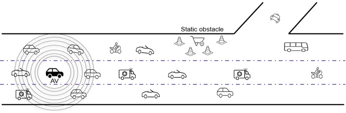
The figure shows that the AV cannot sense the static obstacles present in the top row, which influences the traffic on the left lane. The AV can detect the current and past poses of static/dynamic objects in the scene using its sensor information. Based on these observations, the AV needs to anticipate the neighbour’s intentions (contextual information) and plan its manoeuvre accordingly. This planned manoeuvre should be safe (without colliding with other vehicles), follow the standard traffic rules, and also be energy efficient. The problem of manoeuvre planning (i.e., action taken by the AV without colliding with other objects) by understanding the intentions of its neighbours is referred to as the predictive manoeuvre planning problem. It is assumed that the AV is equipped with an algorithm that can detect the relative poses of both the static and dynamic objects. Thus, the AV has complete histories of paths traversed by the dynamic objects present at any given time and is also aware of the local map. The PMP problem is formulated based on the histories of the paths traversed by the dynamic objects present in the scene and also the local map.

Figure 2: A context region with an AV at the centre

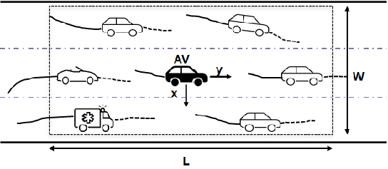
With the above aim, a rectangular window of length $L$ and width $W$ with the AV at the centre is considered, as shown in Figure 2. The past trajectories of the vehicles are represented with dark lines, and the predicted look-ahead trajectories of the dynamic objects (non-ego motion vehicles) are represented using dashed lines. The figure shows the path traversed by AV for the past $n$ frames (${P_{a}}$) and the estimated paths traversed by the other dynamic objects for the past $n$ frames seen at time $t$ (${P_{o}}$). In PMP, it is important to predict the future look-ahead trajectories of the other dynamic objects ($\hat{{P}_{o}}$) to understand the occupancy map into which the AV will move in the near future.

$$\{\textbf{P}_{a}\}=\{(x^{-n}_{a},y^{-n}_{a}),(x^{-n+1}_{a},y^{-n+1}_{a}),...,(x^{0}_{a},y^{0}_{a})\}$$ (1)

$$\{\textbf{P}_{o}\}=\{(x^{-n}_{o_{i}},y^{-n}_{o_{i}}),(x^{-n+1}_{o_{i}},y^{-n+1}_{o_{i}}),...,(x^{0}_{o_{i}},y^{0}_{o_{i}})\}$$

$$\{\hat{\textbf{P}}_{o}\}=\{(\hat{x}^{1}_{o_{i}},\hat{y}^{1}_{o_{i}}),(\hat{x}^{2}_{o_{i}},\hat{y}^{2}_{o_{i}}),...,(\hat{x}^{m}_{o_{i}},\hat{y}^{m}_{o_{i}})\}$$

$$\text{where }i=1,2,...,D;\text{D is number of dynamic objects}$$

The ego vehicle’s action space ($A$) analysis is essentially divided into analysis of longitudinal and lateral maneuver actions. The two decisions for the longitudinal maneuver can be either ’cruise (C)’ or ’brake (B).’ The lateral maneuver action has three possibilities, and it can be either ’keep the same lane’ (S) or ’change to the left lane’ (L), or ’change to the right lane’ (R). The required actions for the AV should also be such that the motion planned by the AV is safe, energy-efficient, and follow the traffic rules.

For solving the problem of PMP, at first, the intentions of surrounding vehicles are inferred from the predicted trajectories of surrounding vehicles. Then it is converted into a classification problem of deciding which decisions to take, and the classification problem is then solved. For every step, both the lateral and longitudinal manoeuvre class’s probabilities have to be predicted as Lat pred = [P(S), P(L), P(R)] and Lon pred = [P(C), P(B)]. Then, the actions with the highest probabilities are chosen from these classification probabilities. In a nutshell, one can say that the PMP problem essentially consists of a trajectory prediction problem followed by a decision classification problem. For carrying out this, as a first step, one needs to encode the context information up to the current instant for the AV and then develop a model to predict the look-ahead occupancy map of the neighbouring dynamic obstacles. Next, one needs to approximate the functional relationships between the context information of the surrounding vehicles and the possible action class for the AV meeting the desired objectives. Since imitation learning [20] tries to mimic the behaviour of humans in different conditions, for PMP, imitation learning from real-world traffic data has been utilized to derive this functional relationship between the context information and the action class. Before getting into the details of the method, a brief description of the traffic datasets used in this study is given next.

II-B Traffic Dataset Description

In this work, the traffic data sets NGSIM I-80 and US-101 [21], where the vehicle positions are given for different time frames, have been used. The two datasets consist of 45 minutes of traffic data at two different locations. Each dataset has three segments of a low, medium, and highly congested traffic data. Each segment has $15$ minutes of traffic data. The datasets are sampled at $10Hz$ implying ten frames per second. The raw dataset gives the positions of all the vehicles and vehicle ids at each time frame. As a first step, to make this raw dataset suitable for prediction purposes, the dataset has to be pre-processed. Each vehicle in the frame is represented as an ego vehicle. If a vehicle’s lane id changed from the previous $4$ seconds to the next $4$ seconds, it was assumed that it changed its lane. From this change in the lane, the lateral manoeuvre done is recorded. Suppose the lane number decreases within this $\pm$ $4$ seconds, then the vehicle changes to the left lane. Otherwise, if the lane number increases in this interval, the vehicle changes to the right lane. Also, if a vehicle’s average speed over the next $5$ seconds is lower than $0.8$ times current speed, it is assumed that the vehicle is braking.

It has also been found that there are some scenarios where the actual decisions taken by a human driver do not satisfy common traffic rules. Hence, if only human decisions are used for learning the possible driving decisions, then the AV can also make unsafe decisions. Hence, there is a need for generating ground truth decisions for each scenario to provide for safe actions. For this reason, ground truth decisions have also been developed in this study for both datasets. More details about ground truth can be found in supplementary document.

II-C Deep Spatio-Temporal Context-Aware decision Network

This paper presents a Deep Spatio-Temporal Context-Aware decision Network referred to as DST-CAN to predict the motion planning actions required for an autonomous vehicle. The schematic diagram of the proposed DST-CAN using context-aware decision making using the PMP model is given in Figure.3. Fig.3 shows that the overall scheme has three major blocks: viz., a perception block, a context generator block, and a CNN decision engine block. The perception engine block of AV detects and tracks other objects. The context generator block generates the current context and future occupancy maps of the neighbouring vehicles. As the final step, based on the above information, the CNN decision engine predicts the manoeuvre decisions which follows the traffic rule with minimum energy. The details of the workings of the different blocks are described next.

Figure 3: A Schematic diagram for PMP using Deep Spatio Temporal Context-Aware decision Network (DST-CAN)

The perception engine in AV identifies the dynamic objects at the current instant and tracks the paths traversed by these objects, as shown in the first block of Figure.3. After the perception engine block, DST-CAN essentially consists of two modules: a context-aware POM generation module using a look ahead predictor and a CNN-based action engine to relate the context frames and action classes. The context-aware POM generator uses the paths traversed by the AV and dynamic objects up to time $t$ and generates their look-ahead trajectories (predictions) using a memory neuron network [11], [10]. A context encoder then encodes these predicted trajectories into a probability occupancy density map. The resultant context and occupancy map frames are then used as inputs to a convolutional neural network to obtain the final motion planning decision (classification).

II-C1 Spatio-temporal Context and probabilistic occupancy map (POM) Generator

The objective of the context and POM encoder is to generate a context and occupancy map in which the autonomous vehicle was present in the past. It also predicts the potential look-ahead trajectories of the other dynamic objects in the scene to understand the future intentions of these objects. The AV perception engine provides the path traversed by the AV (Pa) for n-frames and the paths traversed by the dynamic objects up to the current time frame (Po). Data-driven look-ahead prediction approaches have been widely used for prediction, such as recurrent neural networks [10], long-short term memory networks [22], [23], and fuzzy neural networks [24]. Recently, it was shown that the MNN based approach [10] is effective for look-ahead trajectory prediction than other state-of-the-art approaches.

Hence, in this paper, an MNN has been used and its training has been done with backpropagation in time similar to [10] for look-ahead trajectory predictions. A series-parallel model is used for training, and a parallel-parallel model is used during testing to predict the look-ahead trajectories [25]. From the paths traversed by the dynamic objects ($\{\bf{P}_{o}\}$), changes in displacements in both $x$ and $y$ directions are computed. The inputs to the MNNs are $\Delta x(t-1)$ and $\Delta y(t-1)$, and the outputs of the network are $\Delta x(t)$ and $\Delta y(t)$. The MNN architecture used in the paper is shown in Figure. 4. Each layer has a network neuron (blank circle), and each network neuron has one memory neuron (dark circle). The net output by $\phi_{j}^{h}(t)$ of the $j^{th}$ network neuron in the hidden layer $h$ is:

$$\phi^{h}_{j}(t)=g^{h}\left(\sum_{k=1}^{2}w_{kj}^{i}\psi_{k}^{i}(t)+\sum_{k=1}^{2}f_{kj}^{i}v_{k}^{i}(t)\right)$$ (2)

where,

• $\psi_{k}^{i}(t)$ is the output of the $k^{th}$ network neuron in the input layer $i$. In our case, $\psi_{1}^{i}(t)=\Delta{\hat{x}_{t-1}}$ and $\psi_{2}^{i}(t)=\Delta{\hat{y}_{t-1}}$. $(x,y)$ is position of a vehicle.

• $g^{h}(.)=tanh(.)$ is the activation function of the network neurons present in the hidden layer.

• H is number of network neurons in hidden layer. In this work H=6.

The output of the memory neuron corresponding to the $j^{th}$ network neuron in the layer $l$ is given by:

$$v_{j}^{j}(t)=\alpha_{j}^{l}\psi^{l}_{j}(t-1)+(1-\alpha^{l}_{j})v^{l}_{j}(t-1)$$ (3)

where the $\alpha$ is weight between each network neuron and memory neuron. The net output $n^{L}_{j}(t)$ of the $j^{th}$ network neuron in the last layer $L$ is calculated as:

$$\phi^{L}_{j}(t)=g^{L}\left(\sum_{k=1}^{H}w^{h}_{kj}\psi^{h}_{kj}(t)+\sum_{k=1}^{H}f^{h}_{kj}v^{h}_{k}(t)+\beta^{L}_{j}v^{L}_{j}(t)\right),$$ (4)

where $1\leq j\leq 2$. The inherent feedback connections in the memory neurons help in accurately capturing the dynamics. The network neurons in the hidden layer employ a bipolar sigmoidal activation function, and the output layer employs a linear activation function.

Figure 4: MNN architecture for look-ahead trajectory prediction

The root mean square error function for predicting future positions during training the MNN is given as:

$$RMSE=\frac{\sum_{n=1}^{N}\sqrt{\frac{\sum_{t=1}^{T_{H}}{\lVert\mathbf{x}_{t}^{(n)}-\hat{\mathbf{x}}_{t}^{(n)}\rVert}^{2}}{T_{H}}}}{N}$$ (5)

where $\mathbf{x}_{t}=\left[x(t),y(t)\right]$ and $\hat{\mathbf{x}}_{t}=\left[\hat{x}(t),\hat{y}(t)\right]$ are ground truth and predicted positions respectively. N is the number of vehicles at time t. The network is trained using backpropagation through time algorithm as in [11]. One can find more details on the parallel-parallel implementation used to predict the future $m$-frames, and a comparison with other state-of-the-art method in [10].

Next, the workings of the spatio-temporal context and POM encoder are described. This encoder converts the trajectories of AV and the other dynamic objects in the scene into a context-aware grid. For this purpose, the encoder divides the road segment of length $L$ with AV at the centre into three tracks with equal widths. Further, it divides the road segment into $p$ equal parts. A spatial context map is developed for every past time frame. Since the perception engine gives the distances to the other vehicles very accurately (using sensors like LiDAR), it can be assumed that uncertainty in distance estimation is much smaller compared to each grid length. The grid value on the road segment is set to one if a vehicle occupies the grid. Otherwise, it is set to zero.

(a) context grid map

(b) POM

(c) POM

Figure 5: Context and Probabilistic Occupancy Map (POM) embedding for different time steps

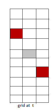
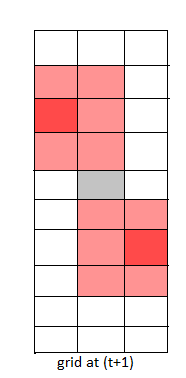
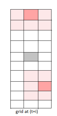
As a typical example, the spatial context map for the current instant is shown in Figure.5(a). The ego vehicle is shown in grey colour. Dynamic objects are shown in red colours. For red colour occupancy, the darker the colour, the higher is the probability of occupancy. There is uncertainty in the predicted positions of surrounding vehicles. The Root Mean Square Error (RMSE) for predictions is given in [10]. To develop a function that can capture the uncertainty well, RMSE for every second has been normalized based on the max error observed. Using this normalized error, a discrete graph showing how certainty reduces with time is shown in Figure.6. A decaying function of time has been fitted to closely relate the uncertainty of prediction to create the POM. This decaying function shows how the certainty of prediction decreases with future time. This decaying function of time is calculated as given below:

$$\textbf{P}(t)=0.47+\sqrt{0.236-0.04\left(\frac{t}{10.0}\right)}$$ (6)

where $0\leq t\leq 50$ is the time index.

Figure 6: Predicted position certainty over different prediction time horizon

Figure 7: Context-aware grid formation and CNN decision engine for AV decision making

1:Inputs: The set of past track history $\{\mathbf{X}_{h}\}_{i=1}^{\mathcal{N}}$ where $\mathcal{N}$ is the number of surrounding vehicles detected by the sensors, pre-trained weights for Memory Neuron Network (MNN), current time step $t$, prediction horizon $T$

2:Output: predicted maneuver $\mathbf{M}$, encoded as a one-hot vector

3:Initialize: $\mathcal{G}$ is a $13\times 3\times 60$ array of zeros

4:Step 1: Obtain the context-aware grid $\mathcal{G}$:

5:for $i\leftarrow 1$ to $\mathcal{N}$ do

6:     for $\tau\leftarrow t-30$ to $t+T$ do

7:         if $\tau\leq$ t then

8:              $\mathcal{G}(i,j,\tau)=1.0$, where $(i,j)$ is the grid
a a aa indices obtained using the relative position $\mathbf{X}_{h}$
a a a . of vehicle $i$ w.r.t ego vehicle’s position at time $\tau$.

9:         else

10:              $\mathcal{G}(i,j,\tau)=\mathbf{P}(\tau)$, where $(i,j)$ is the grid
a a a a indices obtained using the predicted position of
a a a . vehicle $i$ (from MNN), and $\mathbf{P}(\tau)$ is calculated
a a a . using Eq. 6

11:         end if

12:     end for

13:end for

14:Step 2: Calculate the predicted maneuver $\mathbf{M}$ by passing the context aware grid $\mathcal{G}$ to the convolutional social pooling algorithm

Algorithm 1 DST-CAN Context-aware grids generation pseudo code

Based on their past trajectories, POMs are created for the future predicted positions of the surrounding vehicles present at the current instant in the occupancy grid map. The probability that a vehicle will be at the predicted location decreases exponentially with time. The difference in the position of a non-ego vehicle from frame ($t-1$) to frame $t$ is given as an input to the trained MNN. The MNN then outputs the next predicted change in the position. This predicted change in the position is added with the past position to get the next predicted position, as shown in equation 7.

$$\hat{x}_{t+1}=x_{t}+\Delta\hat{x}_{t}\text{ and }\hat{y}_{t+1}=y_{t}+\Delta\hat{y}_{t}$$ (7)

The vehicle will be at that predicted position in the grid with a probability $P(t)$ as given in equation 6 and as shown in 5(b). Since there is always uncertainty in a vehicle’s future predicted position, it is assumed that the vehicle could be at any one of the eight surrounding grids encircled by the MNN predicted grid. It is anticipated that the vehicle could be at any one of the surrounding grids with a probability $(1-P(t))/8$ as shown in Fig.5(b) for the first future frame. Once the first predicted location is found for one future instant, the model takes the change in location from the last time frame and passes that change to the MNN to get the new predicted location change for the second future frame. This new location calculated as a running sum will then have the probability of occupancy calculated according to equation 6 as given by equation 8 (shown in Fig.5(c)).

$$\hat{x}_{t+(i+1)}=\hat{x}_{t+i}+\Delta\hat{x}_{t+i}\text{ and }\hat{y}_{t+(i+1)}=\hat{y}_{t+i}+\Delta\hat{y}_{t+i}$$ (8)

where $i=1,2,...,(m-1)$. A context-aware grid with POM is formed in this way, as shown left part of in Fig.7 for the rest of the prediction horizon. These spatio-temporal context-aware grid frames and POMs are given as input to a convolutional neural network to generate the manoeuvre decisions.

II-C2 Convolutional Neural Network Action Engine

The spatio-temporal context and occupancy map information are embedded into context-aware grid frames and are used to determine the motion planning decisions. Here a convolutional neural network is used to find out the spatial relationships of these vehicles in every frame. The architecture used is shown in the right part of Figure.7. The convolutional neural network employs two three-dimensional convolutional layers and one max-pooling layer. The leaky-ReLU activation function is used for the convolutional layers. The extracted features are flattened and passed through two fully connected networks. The softmax function output gives the probability distribution of lateral and longitudinal motion planning decisions. The mode with the highest probability is chosen as the final decision taken by the ego vehicle.

1:Input: Context Aware Spatio Temporal Grids for every instant as tensors with maneuver decisions (either Ground Truth (GT) decisions or human decisions) at that moment

2:Initialize: Convolutional Neural Network (CNN) with final output dimension of maneuver action classes and a blank list L for storing tensor indexes

3:Step 1: For first epoch, pass all tensors through CNN

4:for $i\leftarrow 1$ to Total number of social tensors do

5:     if predicted decision = actual decision (either GTa  decision or human decision) then

6:         Save the tensor index $i$ to the list L

7:     end if

8:end for

9:Step 2: Remove the tensors in list L from training dataset and get new training dataset with remaining data

10:Step 3: Train the CNN with new training dataset

11:for $i\leftarrow 1$ to E number of epochs do

12:     for $i\leftarrow 1$ to batch size B do

13:         predict the maneuver action classes as probabili a .  a -ties and calculate the Binary Cross Entropy (BCE) a a  loss $\mathcal{L}$ as given in equation 9

14:     end for

15:end for

Algorithm 2 DST-CAN training pseudo code

The training is done with respect to the binary cross-entropy loss given in Eqn.9. The training loss convergence graph for a 3-sec prediction horizon with and without regularization (as described in algorithm 2) is given in Fig.8. The data samples that give good results for the first epoch have been removed from the training dataset for further training for regularizing the training process. It has been found that those samples overfit the DST-CAN model, as shown by the loss curve in Fig.8.

Figure 8: Network training error history

$$\mathcal{L}=-\frac{1}{N}\sum_{i=1}^{N}y_{i}log(p(y_{i}))+(1-y_{i})log(1-p(y_{i}))$$ (9)

where $y_{i}$ is the ground truth and $p(y_{i})$ is the predicted output. $N$ is the total number of samples. The model is implemented in PyTorch[26] and is trained using an RMSProp optimizer.

III Performance Evaluation of DST-CAN

In this section, the performance evaluation results of DST-CAN using benchmark traffic data sets NGSIM I-80, and US-101 datasets [21] are presented. Before presenting the performance results, details of the simulation setup for these studies are described, followed by the performance analysis of DST-CAN for different prediction horizons. Finally, the performance of DST-CAN using a 3-sec prediction horizon is compared with the earlier state-of-the-art approach of Convolutional Social Long-Short Term Memory (CS-LSTM) [17] in terms of correct decision making.

III-A Simulation setup

Publicly available NGSIM US-101 and I-80 datasets [21] have been used for this study. The low and highly congested traffic data from both the datasets have been used for training and the medium congested data for testing. A summary of the details of the datasets is given in supplementary material. For constructing the spatio-temporal grids, the sensor range considered is 90 feet. Each processed data frame consists of vehicles in the range of $\pm$90 feet and two adjacent lanes of the ego vehicle. It is assumed that each lane is 15 feet wide. For prediction, 3 sec of past data is used. Three prediction time horizons consisting of 1 sec, 3 sec, and 5-sec were used to find the one that gave a better result. Most of the data in the datasets correspond to decision-making during cruising in the same lane. Since keeping the same lane manoeuvre is a major portion of the dataset, only a small portion ($20\%$) of those maneuvers are taken for imitative driving model training. By doing this processing, the model can predict lane-changing and longitudinal maneuvers well.

This work here attempts to predict safe and fuel-efficient maneuvers in real scenarios. In this context, if one looks at some of the decisions taken by a human driver, it can be seen that it is not optimal for some situations. Hence ground truth (GT) decisions for every condition have been computed based on simple rule base. For example, to estimate the relative velocity of the vehicle in the front, the vehicle’s position should be tracked for some time. If the front vehicle slows down and there is not enough space for safe driving, it is more reasonable to look for a lane-changing manoeuvre. It should also be checked that there is enough free space to change safely for changing lanes. If at least two grids (i.e., $\sqrt{5}$ in L2 distance from the ego vehicle) are unoccupied on the adjacent lanes on both the forward and rear sides, it is safe to switch the lane. If there is enough space in front of the ego vehicle and the relative velocity of the front vehicle is the same or more than the ego vehicle, then it is safe to cruise on the same lane. If there is not enough space for cruising on the same lane, the ego vehicle should check for the availability of enough space for changing the lanes. If none of the adjacent lanes are free to move safely, then the ego vehicle should brake on the same lane. More details on ground truth decision generation and rules can be found in supplementary document.

Two DST-CAN models, DST-CAN-Imitation and DST-CAN-GT, have been trained to understand the importance of following standard traffic rules. DST-CAN-Imitation is trained with the actual human imitation data and DST-CAN-GT with the ground truth data.

III-B Ablation Study

The trained DST-CAN model has been evaluated using the moderate congestion traffic data. The model finally outputs the probability distribution of the control decisions. The output mode with the highest probability has been taken as the suggested action. That suggested action is given a value of $1.0$, and all other actions are given $0.0$ in the output vector for comparing with the action taken by a human driver. The suggested actions are compared with GT decisions as GT decisions follow the standard traffic rules. There are cases where the decisions taken by humans and GT decisions are conflicting. Since GT decisions are optimal for both safety and fuel efficiency, a comparison has been made with the GT decisions. The percentage of cases when predicted decisions by DST-CAN and GT decisions are the same are compared. Analytical metrics such as root mean squared error, negative log-likelihood, etc., show differences in the results compared to actual human decision data. However, in many cases, human decisions are not good enough, and many of the proposed network predicted decisions could be much better than the actual decisions that human drivers took at that condition. Thus, comparing with the analytical results makes a poor reflection of the model performance. Hence, the percentage of cases where the predicted decisions are the same as ground truth decisions are considered for comparison.

III-B1 Study on prediction horizon

Prediction horizon	Lateral Consensus cases	Lateral Conflict cases	Longitudinal Consensus cases	Longitudinal Conflict cases
	accuracy (%)	accuracy (%)	accuracy (%)	accuracy (%)
1 sec	$99.62$	$13.79$	$95.14$	$32.31$
3 sec	99.67	13.85	95.35	32.81
5 sec	$99.64$	$13.61$	$95.24$	$32.35$

TABLE I: Prediction accuracies for different time horizons

To find the prediction horizon that gives the best result, $1$, $3$, and $5$-seconds horizons were chosen, and detailed studies were undertaken. The comparison results for different horizons are shown in Table I. Consensus cases are those where actual human decisions are the same as the ground truth decisions. Conflict cases are those where the human decisions and ground truth decisions are different. In Table I, the DST-CAN model is trained based only on human decisions. The accuracies for both the consensus and conflict cases are shown in Table I. The results show that the $3$ seconds prediction horizon is better than $1$ second and $5$ seconds prediction horizons. Hence, a $3$ seconds prediction horizon is selected for comparison in this study.

III-B2 Analysis of conflicting cases

(a) $1^{st}$ scene

(b) $2^{nd}$ scene

(c) $3^{rd}$ scene

(d) $4^{th}$ scene

Figure 9: Heat maps of different prediction scenarios

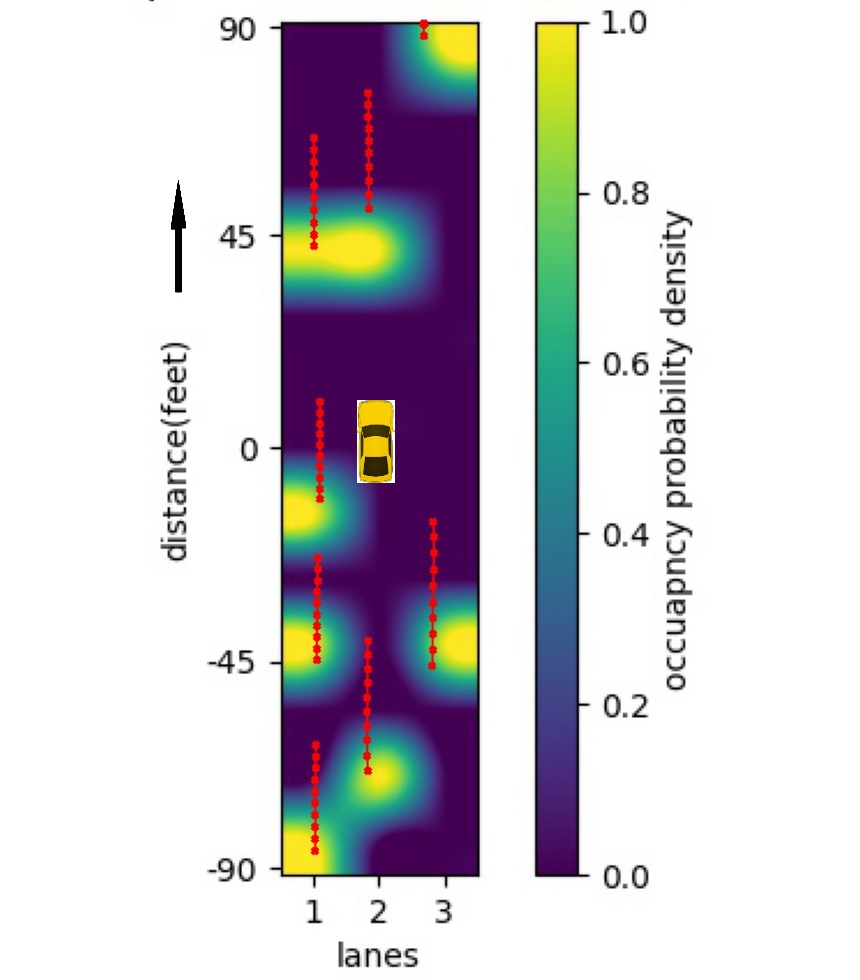
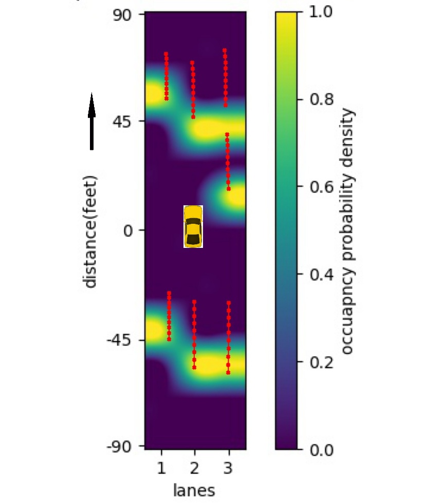
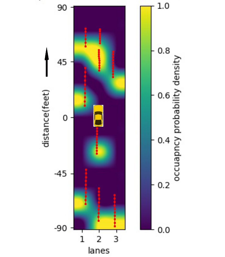
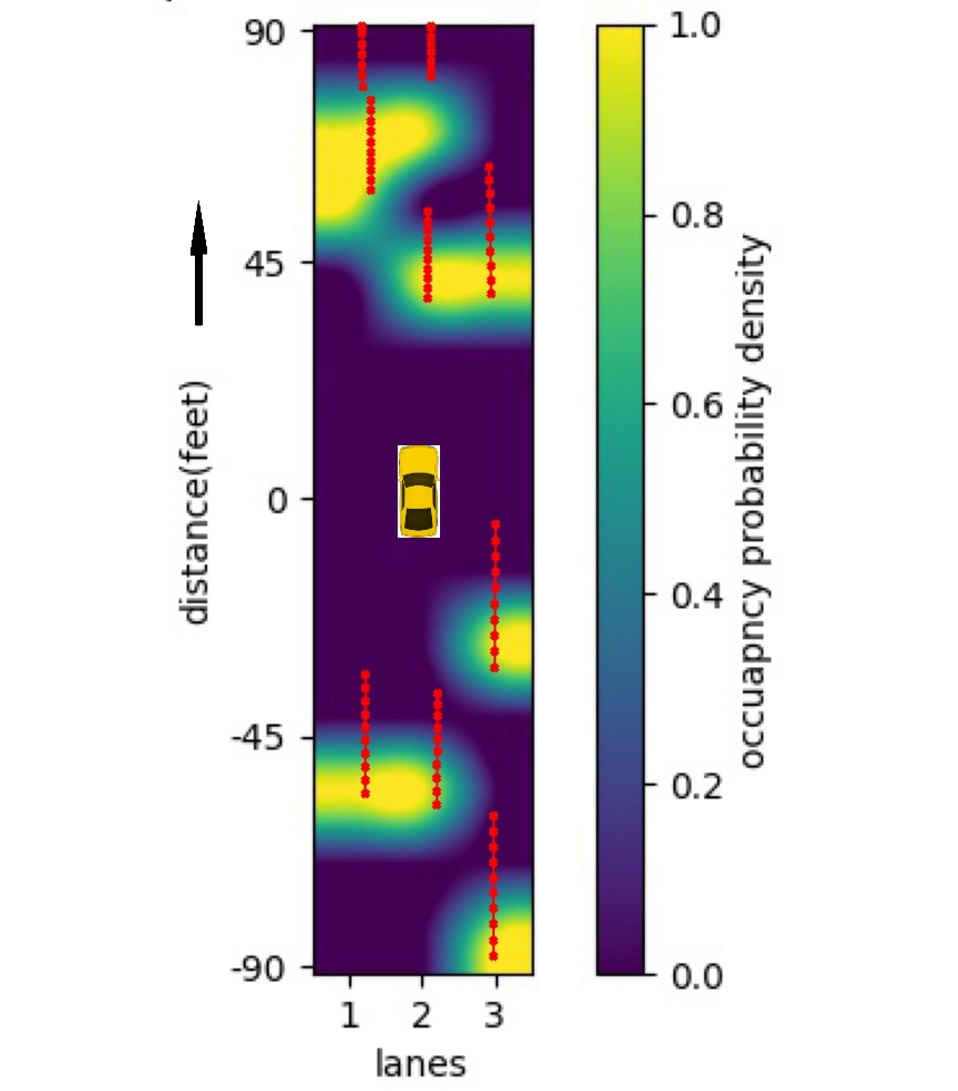
In this section, the cases where the proposed model predicted a different manoeuvre than the actual decision taken by a human driver are analysed. In these cases, the proposed model predicted better control decisions (maneuvers) many times from correctly understanding the behaviours of the surrounding vehicles from their past and the predicted future trajectories. Some of these conditions for mismatching maneuvers are shown in Fig.9. The ego vehicle is at the centre of the heat map, as shown by the yellow vehicle. The heat maps of Fig.9 show the probabilistic occupancy maps of the surrounding vehicles for the immediate next frame. The red dots show the actual trajectories taken by the surrounding cars for ten future frames projected on the heat map to understand the best decision to be taken by the ego vehicle at that instant.

The maneuvers are encoded as one-hot vectors. In Fig.9(a), one probabilistic occupancy grid map is shown. Here DST-CAN predicts an decision that requires it to cruise on the same lane. However, the actual human action taken is braking and changing to the left lane. It may be noted that there is not enough space on the rear side to change to the left lane safely. There is a high chance of collision with another vehicle in the left lane, as can be seen from the red dots on Fig.9(a). Hence, in this case, the human decision is unsafe and inefficient. In this condition, DST-CAN predicts a much better safe and efficient decision. In fig.9(b), another prediction case is shown. Here the model predicts an action to cruise on the same lane. The human driver decided to slow down and move to the left lane. In this case, going to the left lane is safe but not fuel-efficient as the lane in front is free to move. Here DST-CAN’s predicted decision is both safe and fuel-efficient since there is no need for braking. For the scenario shown in Fig.9(c), there will be some space in the left lane to move after some time. Nevertheless, moving to the left lane is not very safe as vehicles are in the rear and forward end of the left lane. Here following the same lane is much safer and more fuel-efficient. There are a few cases where predicted maneuvers based on the DST-CAN are not that good. For example, in Fig.9(d), the human decision is to change to the left lane and cruise. DST-CAN decided to slow down on the same lane. However, one can see from the heat map that cruising on the same lane is the best fuel-efficient manoeuvre.

The reason behind the poor prediction in a few cases is due to that the DST-CAN model proposes a local predictive path planning for an autonomous vehicle. Here global path planning is not of primary concern because the destinations of surrounding vehicles are not known. Sometimes, some surrounding vehicles may maneuver like changing lanes to leave the highway and go to a particular place. The model cannot figure out these conditions very well as it gets trained on such inaccurate data and tries to predict a different decision from the ground truth. These inaccurate data samples cannot be easily removed from the training dataset. For e.g., the vehicle may change lanes to exit a specific highway section without the presence of any surrounding vehicles. The presence of such training samples may affect the generalization ability of the network.

III-C Performance Comparison

Training data used	Lateral Consensus cases		Lateral Conflict cases		Longitudinal Consensus cases		Longitudinal Conflict cases
	DST-CAN(our)	CS-LSTM	DST-CAN(our)	CS-LSTM	DST-CAN(our)	CS-LSTM	DST-CAN(our)	CS-LSTM
Human imitation data	99.67 %	$99.45$%	13.85 %	$8.79$%	95.35 %	$94.72$%	32.81 %	$26.44$%
Ground truth data	99.69 %	$98.11$%	99.82 %	$78.67$%	99.92 %	$97.95$%	99.95 %	$87.83$%

TABLE II: Percentage accuracy comparison for Deep Spatio Temporal Context-Aware decision Network vs. CS-LSTM

In this section, we compare the performance of DST-CAN trained using human imitation decisions and ground truth decision with state-of-the-art approach in the literature [17]. The past $3$ second of trajectory history in the sensing region is used by both DST-CAN and CS-LSTM for predicting the manoeuvre decision. For the implementation of [17] (here), only the model up to lateral and longitudinal manoeuvre prediction has been taken. For training, the model in [17], only low and highly congested traffic data is used. The medium congested data is applied for evaluation. For a fair comparison, two models of CS-LSTM [17] are trained. One CS-LSTM model is trained with human decisions, and the other model with ground truth decisions.

	CS-LSTM prediction							DST-CAN prediction
GT decision	Same lane	Take left	Take right	Cruise	Brake		GT decision	Same lane	Take left	Take right	Cruise	Brake
Same lane	86679	616	3145	0	0		Same lane	89604	582	254	0	0
Take left	46952	104501	3733	0	0		Take left	1	155185	0	0	0
Take right	47648	858	188516	0	0		Take right	3	1	237018	0	0
Cruise	0	0	0	303517	7287		Cruise	0	0	0	310698	106
Brake	0	0	0	74841	289404		Brake	0	0	0	664	363581
	a) Confusion matrix for CS-LSTM							b) Confusion matrix for DST-CAN

TABLE III: Performance comparison based on confusion matrix for conflict scenarios for DST-CAN and CS-LSTM

	CS-LSTM prediction							DST-CAN prediction
GT decision	Same lane	Take left	Take right	Cruise	Brake		GT decision	Same lane	Take left	Take right	Cruise	Brake
Same lane	2405634	13781	30158	0	0		Same lane	2443422	5059	1092	0	0
Take left	1149	2851	93	0	0		Take left	0	4093	0	0	0
Take right	1419	7	2838	0	0		Take right	1	0	4263	0	0
Cruise	0	0	0	2038301	14878		Cruise	0	0	0	2052489	690
Brake	0	0	0	31570	180780		Brake	0	0	0	271	212079
	a) Confusion matrix for CS-LSTM							b) Confusion matrix for DST-CAN

TABLE IV: Performance comparison based on confusion matrix for consensus scenarios for DST-CAN and CS-LSTM

From the ground truth decisions at every time step, the cases where human decisions and ground truth decisions are different have been found. Since ground truth decisions are optimal for both safety and fuel efficiency, these are used for comparison. It has been found that the DST-CAN can predict better decisions than CS-LSTM [17]. Table II shows a comparison of the results. From the table, it is clear that for the consensus cases, the performance of DST-CAN is slightly better than the CS-LSTM. It has been found that conflicting cases are those where safety is of significant importance. DST-CAN performs much better than CS-LSTM for conflicting cases. For the model trained with ground truth decisions, there is a $21.15$ $\%$ and 12.12$\%$ improvement in making correct decisions for conflicting cases for lateral and longitudinal cases, respectively. There are $5.06\%$ and $6.37\%$ improvements for lateral and longitudinal decisions for a model trained with human decisions. Class-wise maneuver predictions are also shown to understand the significance of the proposed model. Table III show the different class-wise predictions for conflicting cases for DST-CAN and CS-LSTM models trained with ground truth decisions. Those tables show the number of samples that are classified in the corresponding classes. From the lane-changing maneuvers, it is clear that DST-CAN performed much better than CS-LSTM. CS-LSTM predicts the decision of following the same lane for many scenes where it should actually predict changing lanes, as it can be seen from Table III. The tables clearly show that DST-CAN predicts fewer misclassifications than the CS-LSTM model. Similarly, Table IV show misclassifications for consensus cases. From tables for consensus cases, it is clear that even with an imbalance in the number of samples for different decisions classes, the self-regulation in learning of DST-CAN helps in better performance than CS-LSTM. From the study, one can say that the proposed DST-CAN accurately predicts safe and efficient lateral and longitudinal decisions based on real traffic conditions.

IV CONCLUSIONS

This paper has presented a novel Deep Spatio Temporal Context-Aware decision Network (DST-CAN), for predictive manoeuvre planning for autonomous vehicles. The surrounding vehicles’ past, present, and accurately predicted future trajectories have been encoded into a context grid in a probabilistic manner. From these encoding, safe and fuel-efficient maneuvers for an AV are predicted. Based on the studies, it was found that human decisions are not safe and fuel-efficient for many scenarios. Hence, to ensure the above ground truth decisions have been developed and are employed for comparison with the earlier proposed CS-LSTM method. From the ablation study of prediction horizons, it has been found that a $3sec$ prediction horizon gives the best result. The study results also show that DST-CAN shows a $21.15\%$ improvement the number of correct lateral decisions and $12.12\%$ improvement for correct longitudinal decisions compared to CS-LSTM. The results clearly indicate the importance of predicting other vehicles’ intentions for good motion planning decisions.

V Supplementary material

A summary of the details of the datasets is given in Table V. The ground truth decision generation details are given in Algorithm 3.

	US101	US101	US101
	07:50-08:05	08:05:08:20	08:20-08:35
Follow same lane	94.19 %	95.78 %	95.93 %
Take left lane	3.70 %	2.67 %	2.91 %
Take right lane	2.11 %	1.55 %	1.16 %
Cruise on same lane	90.49 %	85.96 %	83.19 %
Brake	9.51 %	14.04 %	16.81 %
Total samples	1180598	1403095	1515240
	I80	I80	I80
	16:00-16:15	17:00-17:15	17:15-17:30
Follow same lane	94.37 %	95.87 %	96.17 %
Take left lane	4.62 %	3.60 %	3.19 %
Take right lane	1.01 %	0.53 %	0.64 %
Cruise on same lane	84.58 %	78.77 %	78.17 %
Brake	15.42 %	21.23 %	21.83 %
Total samples	1262678	1549918	1753791

TABLE V: Details of NGSIM traffic dataset

1:Inputs: Social occupancy grid map at current time. $D_{S}$: number of unoccupied grids on the same lane as ego vehicle at current instant; $D_{pre}$: number of unoccupied grids on the same lane as ego vehicle at 2 seconds ago (for relative velocity of vehicle in front of ego vehicle); $D_{LB}$: L2 distance to nearest occupied grid in left-backward side; $D_{LF}$: L2 distance to nearest occupied grid in left-forward side; $D_{RB}$: L2 distance to nearest occupied grid in right-backward side; $D_{RF}$: L2 distance to nearest occupied grid in right-forward side; $I_{r}$: Occupancy of immediate right grid of ego vehicle(1 if occupied, 0 otherwise); $I_{l}$: Occupancy of immediate left grid of ego vehicle(1 if occupied, 0 otherwise)  

2:Output: Ground truth decision at current time  

3:$D_{diff}=D_{s}-D_{pre}$ 

4:if $D_{S}>2$ then

5:     if $D_{diff}\geq 0$ then

6:          lateral decision $\leftarrow$ Follow same lane;
a . . .. . . longitudinal decision $\leftarrow$ Cruise;

7:     else

8:         if [$D_{LB}>\sqrt{5}$ & $D_{LF}>\sqrt{5}$ & ($D_{RB}<=\sqrt{5}$ a . . . . . . . or $D_{RF}<=\sqrt{5}$ or $I_{r}=1$) & $I_{l}=0$] then

9:               lateral decision $\leftarrow$ Take left lane;
a . . .. . a . longitudinal decision $\leftarrow$ Cruise;

10:         else if [$D_{RB}>\sqrt{5}$ & $D_{RF}>\sqrt{5}$ & ($D_{LB}<=\phantom{a}\phantom{a}\phantom{a}\phantom{a}\phantom{a}\phantom{a}\sqrt{5}$ or $D_{LF}<=\sqrt{5}$ or $I_{l}=1$) & $I_{r}=0$] then

11:               lateral decision $\leftarrow$ Take right lane;
a . . .. . a . longitudinal decision $\leftarrow$ Cruise;

12:         else if [($D_{RB}>\sqrt{5}$ & $D_{RF}>\sqrt{5}$) & ($D_{LB}>\phantom{a}\phantom{a}\phantom{a}\phantom{a}\phantom{a}\phantom{a}\sqrt{5}$ & $D_{LF}>\sqrt{5}$) & $I_{r}=0$ & $I_{l}=0$] then

13:               lateral decision $\leftarrow$ Take right lane;
a . . .. . a . longitudinal decision $\leftarrow$ Cruise;

14:         else

15:               lateral decision $\leftarrow$ Follow same lane;
a . . .. . a . longitudinal decision $\leftarrow$ Brake;

16:         end if

17:     end if

18:else

19:     if [$D_{LB}>\sqrt{5}$ & $D_{LF}>\sqrt{5}$ & ($D_{RB}<=\sqrt{5}$ a . . . . . . . or $D_{RF}<=\sqrt{5}$ or $I_{r}=1$) & $I_{l}=0$] then

20:          lateral decision $\leftarrow$ Take left lane;
a . . .. . a longitudinal decision $\leftarrow$ Cruise;

21:     else if [$D_{RB}>\sqrt{5}$ & $D_{RF}>\sqrt{5}$ & ($D_{LB}<=\phantom{a}\phantom{a}\phantom{a}\phantom{a}\phantom{a}\phantom{a}\sqrt{5}$ or $D_{LF}<=\sqrt{5}$ or $I_{l}=1$) & $I_{r}=0$] then

22:          lateral decision $\leftarrow$ Take right lane;
a . . .. . a longitudinal decision $\leftarrow$ Cruise;

23:     else if [($D_{RB}>\sqrt{5}$ & $D_{RF}>\sqrt{5}$) & ($D_{LB}>\phantom{a}\phantom{a}\phantom{a}\phantom{a}\phantom{a}\phantom{a}\sqrt{5}$ & $D_{LF}>\sqrt{5}$) & $I_{r}=0$ & $I_{l}=0$] then

24:          lateral decision $\leftarrow$ Take right lane;
a . . .. . a longitudinal decision $\leftarrow$ Cruise;

25:     else

26:          lateral decision $\leftarrow$ Follow same lane;
a . . .. . . longitudinal decision $\leftarrow$ Brake;

27:     end if

28:end if

Algorithm 3 Ground truth generation pseudo-code

References

- [1] P. Voigtlaender, M. Krause, A. Osep, J. Luiten, B. B. G. Sekar, A. Geiger, and B. Leibe, “Mots: Multi-object tracking and segmentation,” in Proceedings of the IEEE/CVF Conference on Computer Vision and Pattern Recognition (CVPR), June 2019.
- [2] E. Baser, V. Balasubramanian, P. Bhattacharyya, and K. Czarnecki, “Fantrack: 3d multi-object tracking with feature association network,” in 2019 IEEE Intelligent Vehicles Symposium (IV), 2019, pp. 1426–1433.
- [3] C. Luo, X. Yang, and A. Yuille, “Exploring simple 3d multi-object tracking for autonomous driving,” in Proceedings of the IEEE/CVF International Conference on Computer Vision (ICCV), October 2021, pp. 10 488–10 497.
- [4] W. Zhang, H. Zhou, S. Sun, Z. Wang, J. Shi, and C. C. Loy, “Robust multi-modality multi-object tracking,” in Proceedings of the IEEE/CVF International Conference on Computer Vision (ICCV), October 2019.
- [5] A. T. McCartt, V. S. Northrup, and R. A. Retting, “Types and characteristics of ramp-related motor vehicle crashes on urban interstate roadways in northern virginia,” Journal of Safety Research, vol. 35, no. 1, pp. 107–114, 2004.
- [6] U. D. o. T. National Highway Traffic Safety Administration, “Analysis of lane-change crashes and near-crashes,” 2009.
- [7] S. H. Park, B. Kim, C. M. Kang, C. C. Chung, and J. W. Choi, “Sequence-to-sequence prediction of vehicle trajectory via lstm encoder-decoder architecture,” in 2018 IEEE Intelligent Vehicles Symposium (IV), 2018, pp. 1672–1678.
- [8] L. Hou, L. Xin, S. E. Li, B. Cheng, and W. Wang, “Interactive trajectory prediction of surrounding road users for autonomous driving using structural-lstm network,” IEEE Transactions on Intelligent Transportation Systems, vol. 21, no. 11, pp. 4615–4625, 2020.
- [9] A. Zyner, S. Worrall, and E. Nebot, “Naturalistic driver intention and path prediction using recurrent neural networks,” IEEE Transactions on Intelligent Transportation Systems, vol. 21, no. 4, pp. 1584–1594, 2020.
- [10] N. Rao and S. Sundaram, “Spatio-temporal look-ahead trajectory prediction using memory neural network,” in 2021 International Joint Conference on Neural Networks (IJCNN), 2021, pp. 1–8.
- [11] P. Sastry, G. Santharam, and K. Unnikrishnan, “Memory neuron networks for identification and control of dynamical systems,” IEEE transactions on neural networks, vol. 5, no. 2, pp. 306–319, 1994.
- [12] Y. Zhang, W. Wang, R. Bonatti, D. Maturana, and S. Scherer, “Integrating kinematics and environment context into deep inverse reinforcement learning for predicting off-road vehicle trajectories,” arXiv preprint arXiv:1810.07225, 2018.
- [13] D. Choi, T.-H. An, K. Ahn, and J. Choi, “Future trajectory prediction via rnn and maximum margin inverse reinforcement learning,” in 2018 17th IEEE International Conference on Machine Learning and Applications (ICMLA). IEEE, 2018, pp. 125–130.
- [14] P. Wang, C.-Y. Chan, and A. de La Fortelle, “A reinforcement learning based approach for automated lane change maneuvers,” in 2018 IEEE Intelligent Vehicles Symposium (IV), 2018, pp. 1379–1384.
- [15] C. Chen, J. Qian, H. Yao, J. Luo, H. Zhang, and W. Liu, “Towards comprehensive maneuver decisions for lane change using reinforcement learning,” 2018.
- [16] D. Lee, Y. P. Kwon, S. McMains, and J. K. Hedrick, “Convolution neural network-based lane change intention prediction of surrounding vehicles for acc,” in 2017 IEEE 20th International Conference on Intelligent Transportation Systems (ITSC), 2017, pp. 1–6.
- [17] N. Deo and M. M. Trivedi, “Convolutional social pooling for vehicle trajectory prediction,” in Proceedings of the IEEE Conference on Computer Vision and Pattern Recognition Workshops, 2018, pp. 1468–1476.
- [18] A. Alahi, K. Goel, V. Ramanathan, A. Robicquet, L. Fei-Fei, and S. Savarese, “Social lstm: Human trajectory prediction in crowded spaces,” in Proceedings of the IEEE conference on computer vision and pattern recognition, 2016, pp. 961–971.
- [19] B. Mersch, T. Höllen, K. Zhao, C. Stachniss, and R. Roscher, “Maneuver-based trajectory prediction for self-driving cars using spatio-temporal convolutional networks,” in 2021 IEEE/RSJ International Conference on Intelligent Robots and Systems (IROS), 2021, pp. 4888–4895.
- [20] M. Bojarski, D. D. Testa, D. Dworakowski, B. Firner, B. Flepp, P. Goyal, L. D. Jackel, M. Monfort, U. Muller, J. Zhang, X. Zhang, J. Zhao, and K. Zieba, “End to end learning for self-driving cars,” CoRR, vol. abs/1604.07316, 2016.
- [21] J. Colyar and J. Halkias, “Us highway 101 dataset,” Federal Highway Administration (FHWA), Tech. Rep. FHWA-HRT-07-030, 2007.
- [22] A. Zyner, S. Worrall, J. Ward, and E. Nebot, “Long short term memory for driver intent prediction,” in 2017 IEEE Intelligent Vehicles Symposium (IV). IEEE, 2017, pp. 1484–1489.
- [23] F. Altché and A. de La Fortelle, “An lstm network for highway trajectory prediction,” in 2017 IEEE 20th International Conference on Intelligent Transportation Systems (ITSC). IEEE, 2017, pp. 353–359.
- [24] S. Subhrajit, P. Mahardhika, and S. Sundaram, “Bayesian neuro-fuzzy inference system (banfis) for temporal dependency estimation,” IEEE Transactions on Fuzzy Systems, 2020.
- [25] V. Kumar, O. S N, R. Ganguli, P. Sampath, and S. Suresh, “Identification of helicopter dynamics using recurrent neural networks and flight data,” JOURNAL OF THE AMERICAN HELICOPTER SOCIETY, vol. 51, pp. 164–174, 04 2006.
- [26] A. Paszke, S. Gross, F. Massa, A. Lerer, J. Bradbury, G. Chanan, T. Killeen, Z. Lin, N. Gimelshein, L. Antiga, A. Desmaison, A. Kopf, E. Yang, Z. DeVito, M. Raison, A. Tejani, S. Chilamkurthy, B. Steiner, L. Fang, J. Bai, and S. Chintala, “Pytorch: An imperative style, high-performance deep learning library,” in Advances in Neural Information Processing Systems 32, H. Wallach, H. Larochelle, A. Beygelzimer, F. d'Alché-Buc, E. Fox, and R. Garnett, Eds. Curran Associates, Inc., 2019, pp. 8024–8035.