Neural Additive Models for Nowcasting

Abstract

Deep neural networks (DNNs) are one of the most highlighted methods in machine learning. However, as DNNs are black-box models, they lack explanatory power for their predictions. Recently, neural additive models (NAMs) have been proposed to provide this power while maintaining high prediction performance. In this paper, we propose a novel NAM approach for multivariate nowcasting (NC) problems, which comprise an important focus area of machine learning. For the multivariate time-series data used in NC problems, explanations should be considered for every input value to the variables at distinguishable time steps. By employing generalized additive models, the proposed NAM-NC successfully explains each input value’s importance for multiple variables and time steps. Experimental results involving a toy example and two real-world datasets show that the NAM-NC predicts multivariate time-series data as accurately as state-of-the-art neural networks, while also providing the explanatory importance of each input value. We also examine parameter-sharing networks using NAM-NC to decrease their complexity, and NAM-MC’s hard-tied feature net extracted explanations with good performance.

1 Introduction

Deep neural networks (DNNs) are among the most powerful machine learning tools used for natural language processing [1], image classification [2], sound recognition [3], and more. DNNs are powerful because of their free input and output forms, which other methods lack [4]. This advantage can be applied to real-world time-series data problems, such as nowcasting (NC), which uses a DNN to predict the next time step for power system monitoring [5], rainfall prediction [6], cutting-force prediction, and other problems.

Because DNNs are black-box models, they lack explanatory power behind their predictions. This is a critical issue, as the scientific method requires a good understanding of the system and the causes of the results. Neural additive models (NAMs) have recently been proposed to help explain how DNNs reach their prediction values [7]. NAMs assign targets to feature-net base modules that represent each variable. Then, based on their changes, the reasons for the DNN output are better understood.

In this paper, we propose a novel NAM for multivariate NC problems (NAM-NC) by extending them to explain the predictions of multivariate time-series data. An explanation must be considered for each input value of the variables at all time steps. By employing a generalized additive model (GAM), the proposed NAM-NC successfully explains each input value’s importance. Furthermore, it supports multi-task learning and is suitable for multivariate NC tasks. According to our results, the feature-nets maintain prediction performance, even when the NAMs are configured with fewer than optimal parameters.

This work makes the following contributions:

• GAMs enable NAM-NC to explain NC results after training without additional model-agnostic methods [8].

• Multivariate NC is supported, and each NC is influenced by cross-correlating other time series, including auto-correlations.

• Two-parameter sharing structures reduce NAM-NC’s complexity, and with reduced parameters, its performance is maintained.

• State-of-the-art performance is maintained for time-series NC tasks using real datasets.

We review past works in Section 2. Section 3 introduces NAM-NC and illustrates how it explains the prediction mechanisms of DNNs using synthetic sinusoidal signals. Section 4 explains how to share parameters in NAM-NC. Section 5 uses experimentation to demonstrate the competitiveness of NAM-NC with other time-series DNN methods on a benchmark dataset. This section also visualizes NAM-NC’s calculation methods. Finally, Section 6 concludes this work.

2 Related work

The use of auto-regressive (AR) models to tackle time-series NC problems has long been a key focus of machine learning. The AR model predicts the value of the next time step by calculating the weights that best explain the data in the previous step [9]. The vector AR method was designed for multivariate NC by extending the univariate NC method [10]. Owing to their simplicity, basic AR models can provide predictive interpretations of derivative models that are still in use today [11]. A recent AR project, Prophet, performed univariate NC tasks [12]. There have also been attempts to estimate AR parameters using NN structures [13, 14]. Prophet was later improved to learn traditional statistical solutions this way [15]. Also, time-series NC data are often processed from datasets using non-recursive tabular formats [16].

New NN methods have been introduced to extract the most meaningful vectors from time series. Long short-term memory (LSTM) improves recurrent NNs (RNNs), enabling them to retain meanings extracted from more distant time points [17]. Other studies have attempted to compensate for the shortcomings of LSTM [18, 19, 20]. Meanwhile, attention-based and convolutional NNs (CNNs) have been applied to time-series predictions, showing good performance [21, 22]. The bidirectional-encoder-representations-from-transformers (BERT) model with an attention layer is among the most powerful natural language processing (NLP) tools used today [23]. Notably, the positional encoding used by BERT to convey location information in the attention layer is effective for time-series learning [24]. The Informer application achieved state-of-the-art (SOTA) performance with time-series forecasting by reducing the computational costs of the attention layer and improving positional encoding [5]. A temporal CNN using dilated convolution is a representative model that processes time-series based on a CNN [25, 3]. Recently, SCINet achieved SOTA on benchmark datasets by convolving a binary tree-like hierarchical structure [26].

However, the explainability power of DNN prediction mechanisms has been elusive [27]. Thus, researchers have shown interest in correlating DNN predictions to the variability of machine learning input [28]. Class activation mapping estimates the contributions of input data by relying on the CNN’s receptive field [29]. The temporal LSTM with attention also interprets the time series by employing an attention layer to an RNN structure [30]. Layer-wise relevance propagation suggests the possibility of interpreting DNN results by backtracking the values contributing to the prediction results in the NN graph [31]. The local-interpretable-model-agnostic-explanations model interprets a prediction using hypothetical data close to the predicted data [32]. Meanwhile, GAMs make predictions using contributions extracted by a simple function for each variable in the data [8]. The GAM function is presented in Eq. 1. The GAM uses the base module $f$ that only focuses on one of the $K$ variables for explainable predicting. Because the GAM employs an isolated module $f$ for each variable, the GAM provides the influence of each variable for predicting the target $\hat{y}$.

$$\begin{split}\hat{y}=&\beta+f_{1}(x_{1})+\cdots+f_{K}(x_{K})=\beta+\sum_{k=1}^{K}f_{k}(x_{k})\end{split}$$ (1)

The Shapley additive explanations (SHAP) model describes popular NN methods based on GAM and Shapley theory [33]. In particular, SHAP shows that DNNs can be described as model-agnostic using DeepLift, which compares the activation of each neuron to its reference activation and assigns contribution scores according to the difference [34]. The time-SHAP model further explains LSTMs and reduces the computational cost of kernel-SHAP during explanatory training [35].

3 NAM-NC

NAM extracts features from each variable using a simple feature net. Contrary to recent trends, NAM has produced good results with tabular data, despite being a lightweight network [7, 36]. Thus, we employed the basic premise of NAM and expanded it to handle NC tasks by employing multi-task learning to support predictions based on multivariate time-series data.

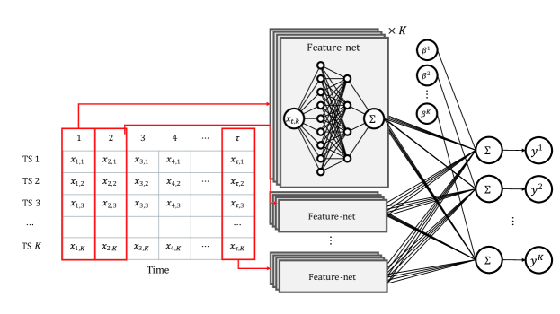
Figure 1 illustrates the structure of NAM-NC for multivariate time-series NC. As shown, the time series, $X_{T-\tau+1:T,K}\in\mathbb{R}^{\tau\times K}$, can be expressed in the form of $K$ variables and with $\tau$ length. Each value, $x_{t,k}$, of the time series, $X$, is input to the feature-net, $f_{t,k}$. Each feature net receives one variable, $x_{k}\in\mathbb{R}^{1}$, and computes one feature scalar, $f_{k}(x_{k})\in\mathbb{R}^{1}$, with the same dimension. The goal of NC is to predict $X_{T+1,K}=Y$ at time $T+1$ based on $X_{T-\tau+1:T,K}$. We can predict the $T+1^{th}$ time step of the $k^{th}$ series by again calculating a linear combination of the extracted feature values and adding them. Thus, Eq. 2 expresses the NC result of Eq. 1:

$$\begin{split}\hat{y}^{K}=\beta^{K}+w^{K}_{1,1}f_{1,1}(x_{1,1})+\cdots+w^{K}_{\tau,K}f_{\tau,K}(x_{\tau,K})=\beta^{K}+\sum_{t=1}^{\tau}\sum_{k=1}^{K}w^{K}_{t,k}f_{t,k}(x_{t,k}).\end{split}$$ (2)

The superscripts of all items in the Eq. 2 specify time-series $K$ among those located at time $T+1$. Eq. 2 provides the process of summing the feature values extracted by the feature net and weighting them according to their location information. The scalar extracted by the feature-net, $f_{t,k}(\cdot)$, is influenced only by the input value, $x_{t,k}$. As the extracted scalar does not combine with other time-series points during training, $f(x)$ is used as the specific input value. Especially, the NAM utilizes the Exp-centered Unit (ExU) as its feature net $f$, which is designed to be sensitive to the contribution of the input [7]. Therefore, NAM-NC can ignore unrelated time-series points. However, these important points can greatly affect prediction outcomes.

Figure 1: Neural additive model for nowcasting.

Next, we provide an analysis of NAM-NC results using simple synthetic time-series toy data consisting of five relevant features and three irrelevant random noise items. The relevant features are generative and combine the sine and cosine functions of different periods and amplitudes. Figure 2 shows the generated time-series data. One of the base time series, TS1, is used as the original, from which we produce two variations. The other time series, TS2 and TS3, are not related. One variation, “.5 x TS 1," only halves the amplitude while retaining the TS1’s period. The other, “Shifted TS 1," employs a periodic shift with the same amplitude as the original. For the experiments, we set $\tau$ to eight for all time series. We applied NAM-NC to the multivariate time-series data, expecting that the relevant features would provide high feature-net outputs and that the irrelevant ones would provide low outputs.

Figure 2: Five synthesized time series and three noises.

Figure 3: Nowcasting performance for eight time series.

Figure 4: Contribution according to the unique value of each time series. The nowcasting target of left and right figure is the TS1 and TS2, respectively.

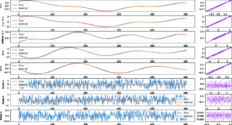
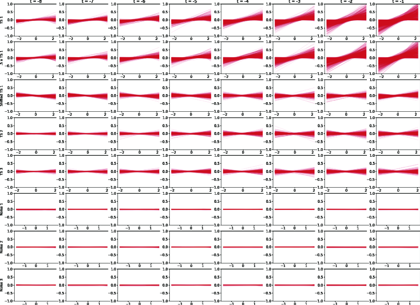
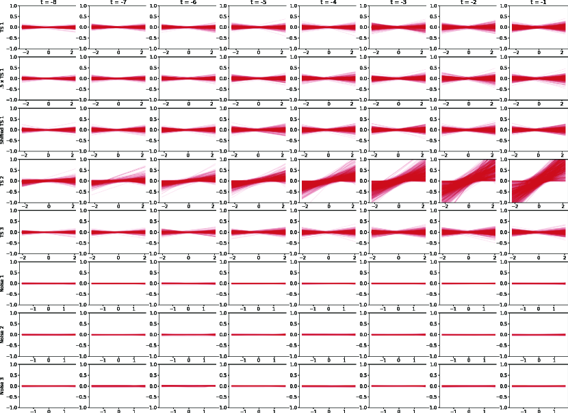
Figure 3 illustrates the NC results of the synthesized time-series data. The sub-figures in the first column indicate each true point in the time series (blue line) and the predicted points of NAM-NC (orange line) in the time step domain. The sub-figures in the second column express the same information as an x- vs. y-axis slope. Thus, it is apparent that NAM-NC can accurately predict multivariate time-series data. Figure 4 illustrates the importance of each time-series point to prediction. NAM-NC employs $\tau\times K$ feature nets to extract the importance from scalar data points for each. Figure 4 illustrates the contributions of $\tau\times K$ input points to TS1 (left) and TS2 (right). Rows and columns indicate each $k$ time series and $t$ step, respectively. The x-axis of the subplots located in each matrix represents the unique values of the input time series, and the y-axis is the value extracted by $f$ dedicated to each point from the unique values of the input. We repeated training 1,000 times using the same structure to check the consistency of NAM-NC. Figure 4 presents all contributions made by passing the unique $k^{th}$ time series through 1,000 times repeat. The red line is translucent to make it easier to see that training was repeated. According to the results, We figured out that the feature net $f_{t,k}$ of NAM-NC nowcasting the time series $k$ produces a smaller contribution as it looks at the distant past time. In TS1’s NC, only the feature scalars extracted from the two time series related to TS1 made significant contributions. Moreover, TS2’s NC only obtained its contributions from the time series to which it belonged. We also found that no NC targets received contributions from noises.

4 NAM-NC parameter sharing

One advantage of NAM is that it is possible to find the sufficient context vector needed for inference from table data, even when using a simple unit network [7]. NAM-NC repeats the number of variables as many times as the value of time-step $\tau$, resulting in a higher computational cost than regular NAM. Therefore, we sought a way to reduce the computational cost of NAM-NC. A simple potential solution is parameter sharing, which in multi-task learning is often used to reduce the weight of NNs [37]. Hard-sharing, which involves sharing most parameters while independently utilizing only the output layer for multi-task learning, can also significantly reduce weight [38]. Thus, we applied hard-sharing in terms of time or features between feature-nets to tie the parameters of NAM-NC. Its formula, as applied to hard-sharing, is shown in the two-part Eq. 3:

$$\begin{split}\hat{y}^{K}_{time}=&\beta^{K}+w^{K}_{1,1}f_{:,1}(x_{1,1})+\cdots+w^{K}_{\tau,K}f_{:,K}(x_{\tau,K})=\beta^{K}+\sum_{t=1}^{\tau}\sum_{k=1}^{K}w^{K}_{t,k}f_{:,k}(x_{t,k})\\ \hat{y}^{K}_{feature}=&\beta^{K}+w^{K}_{1,1}f_{1,:}(x_{1,1})+\cdots+w^{K}_{\tau,K}f_{\tau,:}(x_{\tau,K})=\beta^{K}+\sum_{t=1}^{\tau}\sum_{k=1}^{K}w^{K}_{t,k}f_{t,:}(x_{t,k})\end{split}$$ (3)

Where “:” refers to the dimension with which the parameter is shared. Accordingly, we can reduce the computational cost by sharing feature-net $f$ at each time step or series to increase the computational cost of NAM-NC. Therefore, the space complexity of NAM-NC’s parameters is reduced from $\mathcal{O}(\tau\times K)$ to $\mathcal{O}(\tau)$, or $\mathcal{O}(K)$.

5 Evaluating the performance of the NAM-NC

Here, we compare the NC performance of NAM-NCs to that of other SOTA models using real data. All our experiments are available on the NAM-NC GitHub site. For model comparison, we prepared Informer, for which temporal encoding is applied with positional encoding, and SCINet and LSTM, for which both had the input format required. Temporal encoding was used with Informer to capture the real-time influence of variables. However, as we did not use real-time information for NC, we removed its temporal encoding and kept the positional encoding. SCINet performs convolution by splitting the time series into a binary tree structure. Thus, the length of its input time series must take the format of $2^{n}$. Therefore, we used a time-series input length of eight for all models.

Table 1: Configuration of the experiment.

Model name	Param. name	Set	Param. name		Set
Shared params	Batch-size	128	Early stop round		10
	lr	0.001	Dropout		0.1
NAM-NC	Exu –- linears	[100,32]	LSTM	hidden	100
	Activation	leaky–ReLU		n–layer	2
	Init distribution	$\mathcal{N}(0,1)$		bidirectional	True
Informer	$d_{model}$	64	SCINet	Num levels	3
	n–heads	4		Kernel size	5
	$d_{ff}$	64		Conv hidden	1

Table 1 summarizes the hyperparameters used for the experiment. The top row identifies the categories of the other rows. Specific parameters are shown for each model. Unimportant parameters were set to their default values according to their respective research articles. We employed the Adam optimizer with no weight decay. The feature net of NAM-NC first passes through ExU and then through its linear combination layer [7]. According to NAM, 1,000 nodes of ExU are sufficient to extract the feature scalars from all inputs. However, in our experiment, only 100 nodes of ExU were used. Thus, we extracted the feature scalar from the TS points without using a linear combination multilayer structure. Additionally, a rectified linear unit (ReLU) with a limited maximum value for NAM was used to lower the dependence of specific feature-nets while hindering training the time-series data. Thus, we used a leaky ReLU for NAM-NC’s feature-net activation.

During the time-series cross-validation process, after dividing the time series into $K$ equal parts, the training time series was accumulated from the front, followed by $K$ instances [39]. The subsequent time series for validation was cropped by 10% of its length and used for learning. Figure 5 illustrates the cross-validation process. Next, we set $K$ to 10 for NC validation. We then used the root mean-squared error (RMSE), the mean absolute error (MAE), and $R^{2}$ as criteria for validation. RMSE and MAE reflect the absolute deviation of the error as 2- and 1-norms. We also employed $R^{2}$ as RMSE and MAE do not account for the trend between real and predicted values.

Figure 5: Process of the time series $K$–fold cross-validation.

We used the Electricity Transformer Temperature (ETT) dataset collected from two transformers in two Chinese provinces, one each [5]. Indicators m or h represent intervals of data collected as 15 min or 1 h, respectively. For example, the 15-min interval dataset collected from the first transformer is ETTm1, and each from ETT contains seven time series. The senven time series contain the “UseFul" and “UseLess" Load with three types of power loads (i.e. high, middle and low), and oil temperature. For convenience, we will use abbreviations: high useful loads, high useless loads, middle useful loads, middle useless loads, low useful loads, and low useless loads are HUFL, HULL, MUFL, MULL, LUFL, and LULL, respectively. The ETTh1 and ETTh2 has 17,421 time lengths while ETTm1 and ETTm2 has 69,681 time lengths.

We compared NAM-NCs’ performance to three comparative models. Table 2 shows the experimental NC results for the ETT dataset. The first row indicates the dataset and metric types. The rows below show the metrics of the method used by the province transformer per time interval. In the metric tables, the bold and underline indicates the best scores of all NN methods and NAM-NCs’ variations, respectively. NAM-NCs showed the best performance from the second transformer. NAM-NCs with shared parameters resulted in lower scores in terms of $R^{2}$ compared to the original NAM-NC. However, NAM-NC_feature showed the best performacnes in ETTh2 and ETTm2 in terms of RMSE and MAE. Also, NAM-NC_time showed the best $R^{2}$ in ETTm2. In particular, all NAM-NCs often outperformed other comparison methods. SCINet maintained the performance consistency. SCINet achieved the best performance for all metrics from the first transformer. Meanwhile, LSTM showed the worst performance.

Table 2: Summary of the experiment for ETT dataset

Category	Dataset	Method	$\#$ Params	$R^{2}$	RMSE	MAE	Dataset	Method	$\#$ Params	$R^{2}$	RMSE	MAE
ETT	ETTh1	NAM-NC	193k	0.7474	1.4004	0.7954	ETTm1	NAM-NC	193k	0.8997	0.8350	0.4424
		NAM-NCtime	24k	0.7434	1.4172	0.8065		NAM-NCtime	24k	0.8932	0.8571	0.4553
		NAM-NCfeature	28k	0.7432	1.4054	0.7973		NAM-NCfeature	28k	0.8986	0.8442	0.4466
		Informer	330k	0.7407	1.3598	0.7860		Informer	330k	0.8874	0.8946	0.4736
		LSTM	188k	0.7006	1.4385	0.8387		LSTM	188k	0.8793	0.8950	0.4856
		SCINet	11k	0.7695	1.3093	0.7338		SCINet	11k	0.9037	0.8092	0.4168
	ETTh2	NAM-NC	193k	0.6289	2.0359	1.2897	ETTm2	NAM-NC	193k	0.8250	1.3256	0.7981
		NAM-NCtime	24k	0.6162	2.0188	1.3013		NAM-NCtime	24k	0.8272	1.2147	0.7750
		NAM-NCfeature	28k	0.6134	1.9767	1.2847		NAM-NCfeature	27k	0.8259	1.1950	0.7591
		Informer	330k	0.5856	2.3137	1.4151		Informer	330k	0.7781	1.6681	0.9368
		LSTM	188k	0.5041	2.7676	1.7218		LSTM	188k	0.7582	1.7746	1.0120
		SCINet	11k	0.6123	2.1666	1.3356		SCINet	11k	0.8050	1.4351	0.8272

(a) HUFL

(b) HULL

(c) MUFL

(d) MULL

(e) LUFL

(f) LULL

Figure 6: Contribution of the unique values in time series of the ETTh1 datasets when to predict the next time step’s value. The subfigure’s caption indicates the nowcasting target.

Figure 7: Importance value of each input variable for each target of ETTh1.

Table 3: Summary of the experiment for BAQ time series datasets.

Category	Dataset	Method	$\#$ Params	$R^{2}$	RMSE	MAE	Dataset	Method	$\#$ Params	$R^{2}$	RMSE	MAE
BAQ	Aotizhongxin	NAM-NC	275k	0.8651	105.23	23.21	Nongzhanhuan	NAM-NC	275k	0.8742	105.73	23.19
		NAM-NCtime	35k	0.8599	105.27	23.35		NAM-NCtime	35k	0.8719	106.34	23.61
		NAM-NCfeature	28k	0.8669	104.88	23.10		NAM-NCfeature	28k	0.8760	105.63	23.02
		Informer	333k	0.8569	112.36	24.21		Informer	333k	0.8705	110.60	24.49
		LSTM	189k	0.8538	107.86	23.83		LSTM	189k	0.8696	106.98	23.72
		SCINet	23k	0.8768	103.64	22.04		SCINet	23k	0.8864	103.62	21.83
	Changping	NAM-NC	275k	0.8337	110.00	24.95	Shunyi	NAM-NC	275k	0.8438	108.42	23.53
		NAM-NCtime	35k	0.8321	110.38	25.14		NAM-NCtime	35k	0.8514	106.38	23.08
		NAM-NCfeature	28k	0.8372	109.75	24.68		NAM-NCfeature	28k	0.8547	107.17	22.91
		Informer	333k	0.8356	109.56	25.09		Informer	333k	0.8337	116.99	24.59
		LSTM	189k	0.8323	109.61	24.66		LSTM	189k	0.8184	115.98	24.43
		SCINet	23k	0.8493	106.10	23.36		SCINet	23k	0.8532	108.34	22.21
	Dingling	NAM-NC	275k	0.8633	76.98	16.99	Tiantan	NAM-NC	275k	0.8544	106.69	23.06
		NAM-NCtime	35k	0.8607	77.15	17.34		NAM-NCtime	35k	0.8501	106.68	23.57
		NAM-NCfeature	28k	0.8644	76.86	16.84		NAM-NCfeature	28k	0.8540	106.15	22.95
		Informer	333k	0.8588	78.78	17.55		Informer	333k	0.8512	106.63	23.11
		LSTM	189k	0.8565	80.31	18.13		LSTM	189k	0.8507	106.22	23.17
		SCINet	23k	0.8758	75.64	15.86		SCINet	23k	0.8667	102.64	21.64
	Dongsi	NAM-NC	275k	-0.4103	94.25	21.30	Wanliu	NAM-NC	275k	0.8611	97.05	21.80
		NAM-NCtime	35k	-0.5088	94.85	21.61		NAM-NCtime	35k	0.8582	99.02	22.86
		NAM-NCfeature	28k	0.0755	93.72	20.88		NAM-NCfeature	28k	0.8650	97.02	22.09
		Informer	333k	-1.3288	97.13	22.02		Informer	333k	0.8516	100.70	23.44
		LSTM	189k	0.1420	99.00	22.40		LSTM	189k	0.8496	103.30	24.19
		SCINet	23k	0.4657	92.85	19.99		SCINet	23k	0.8755	93.91	20.61
	Guanyuan	NAM-NC	275k	0.8670	95.32	21.05	Wanshouxigong	NAM-NC	275k	0.8525	104.28	24.76
		NAM-NCtime	35k	0.8665	94.54	21.25		NAM-NCtime	35k	0.8500	104.57	24.92
		NAM-NCfeature	28k	0.8702	94.90	21.03		NAM-NCfeature	28k	0.8535	104.54	24.63
		Informer	333k	0.8658	99.45	22.02		Informer	333k	0.8472	104.83	24.95
		LSTM	189k	0.8621	96.93	21.81		LSTM	189k	0.8433	103.80	24.78
		SCINet	23k	0.8798	92.15	19.70		SCINet	23k	0.8661	100.32	23.02
	Gucheng	NAM-NC	275k	0.8353	99.85	24.16	Huairou	NAM-NC	275k	0.8415	82.04	19.21
		NAM-NCtime	35k	0.8362	99.78	24.26		NAM-NCtime	35k	0.8369	82.23	19.63
		NAM-NCfeature	28k	0.8440	99.50	23.83		NAM-NCfeature	28k	0.8400	82.23	19.23
		Informer	333k	0.8367	100.95	25.03		Informer	333k	0.8350	84.02	19.43
		LSTM	189k	0.8315	104.70	25.79		LSTM	189k	0.8353	82.22	19.52
		SCINet	23k	0.8530	97.76	22.48		SCINet	23k	0.8567	79.68	18.04

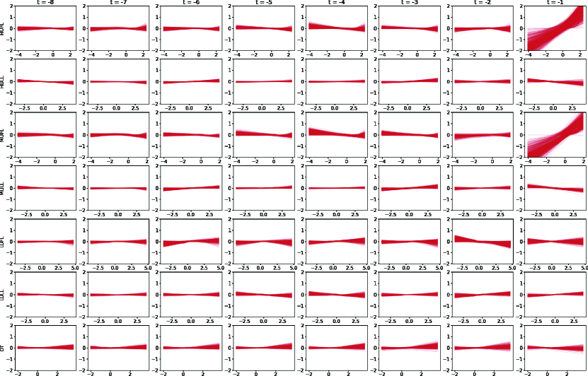
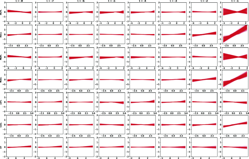
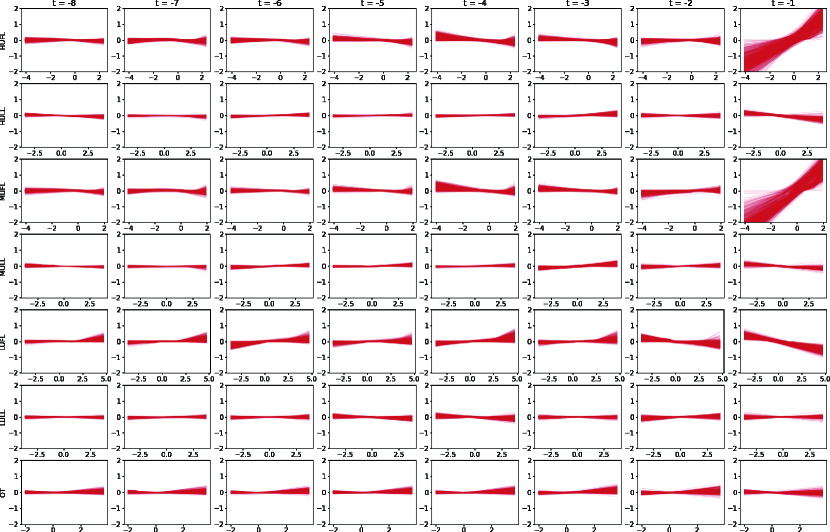
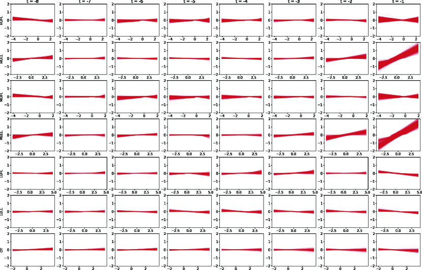
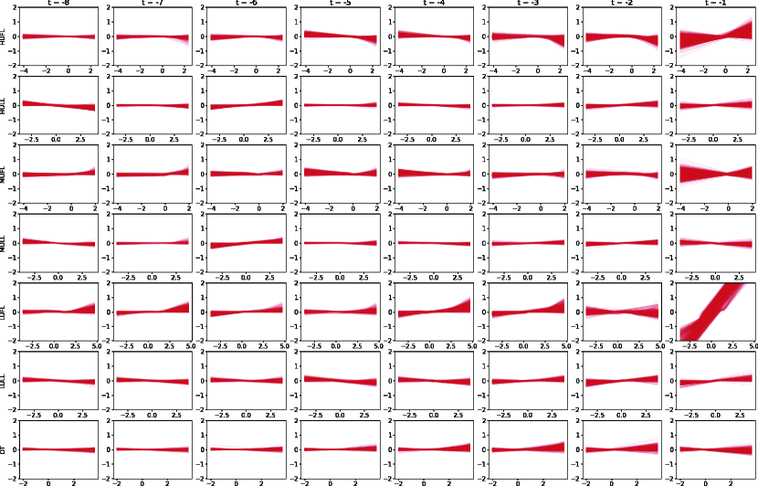
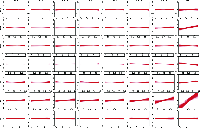
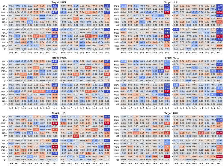
Unlike other methods, our model can explain how an NN makes its predictions. Figure 6 visualizes the scalar extracted by NAM-NC’s feature net from the ETTh1 dataset. The feature scalars of the unique values of each time series in ETTh1 extracted by the feature net revealed large deviations from the input time series immediately prior to NC. We also found a strong correlation between HUFL and MUFL and between HULL and MULL, according to the unique inputs. We further confirmed a similar pattern in the time-series samples of ETTh1. Figure 7 shows the contributions generated by the feature net of NAM-NC trained four times to repeat each NC target. According to the figure, each trained model extracted contributions by ignoring unimportant time-series points and focusing on critical points. Furthermore, NAM-NC did not always obtain the contribution information from the immediately preceding item; it also extracted contributions from the distant past.

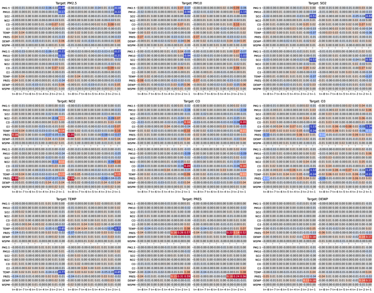
We employed another dataset: Beijing Air Quality (BAQ) [40]. All BAQ time-series data consist of 10 time series contain to air quality, $SO_{2}$, and more. Objects with time lengths of 35,065, the size of fine dust, are contained in the set, including temperature, humidity, etc., taken from monitoring sites near Beiging. According to Table 3, NAM-NC_feature performed the best in most metrics among NAM-NCs. It is seemed that NAM-NCs with shared parameters provide computational efficiency, but do not degraded the prediction performance. SCINet showed the best prediction performance for most datasets; however the NAM-NCs showed comparable results while providing the explanation power. Figure 8 shows the contributions generated by the feature net of NAM-NC trained four times to repeat each NC target of BAQ. According to the figure, NAM-NC captured the time series which is correlated, as temperature, pressure, and dew point. Also, we explained the NAM-NC’s prediction for the $NO_{2}$ and $O_{3}$ that received the contribution from the distant past, such as pressure at $t=-8$.

Figure 8: Importance value of each input variable for each target in BAQ’s Shunyi site.

6 Conclusion

Despite its nonrecursive structure, NAM-NC supports NC tasks well. Owing to its GAM basis, NAM-NC can explain prediction results on both synthetic and real datasets. We used hard sharing to reduce the number of parameters, and NAM-NC performed just as well as before parameter grouping, although the number of parameters was considerably reduced. To show the explainability of NAM-NC, we visualized its predictions using feature nets for unique values in synthetic data. Both synthetic and real time-series data were used, and NAM-NC extracted the tendency contributions of the unique time-series inputs. Even with repeated learning, we confirmed the model’s consistency in extracting most of the large contributions from the important points identified in the time series data. Therefore, NAM-NC has a competitive edge over other NN models due to its explainability under the assumption that it learns and predicts fields that support NC tasks.

NAM-NC still faces several obstacles. In this study, hyperparameters were not specifically explored, and we did not utilize the various time-series lengths. Therefore, it is necessary to verify NAM-NC with other types of datasets. The model showed good performance in the ETT and BAQ problems, which have strong periodicity. Thus, the recursion of NNs based on scalars extracted by feature nets requires more attention. Additionally, researchers should expand the scope of NAM-NC beyond recursion into forecasting.

References

- [1] Clark, K., M.-T. Luong, Q. V. Le, et al. ELECTRA: Pre-training text encoders as discriminators rather than generators. In ICLR. 2020.
- [2] Redmon, J., A. Farhadi. Yolov3: An incremental improvement. ArXiv, abs/1804.02767, 2018.
- [3] Lea, C., M. D. Flynn, R. Vidal, et al. Temporal convolutional networks for action segmentation and detection. In 2017 IEEE Conference on Computer Vision and Pattern Recognition (CVPR), pages 1003–1012. 2017.
- [4] Tu, J. V. Advantages and disadvantages of using artificial neural networks versus logistic regression for predicting medical outcomes. J Clin Epidemiol, 49(11):1225–1231, 1996.
- [5] Zhou, H., S. Zhang, J. Peng, et al. Informer: Beyond efficient transformer for long sequence time-series forecasting. In AAAI. 2021.
- [6] Ridwan, W. M., M. Sapitang, A. Aziz, et al. Rainfall forecasting model using machine learning methods: Case study terengganu, malaysia. Ain Shams Engineering Journal, 12(2):1651–1663, 2021.
- [7] Agarwal, R., L. Melnick, N. Frosst, et al. Neural additive models: Interpretable machine learning with neural nets. In A. Beygelzimer, Y. Dauphin, P. Liang, J. W. Vaughan, eds., Advances in Neural Information Processing Systems. 2021.
- [8] Hastie, T., R. Tibshirani. Generalized additive models. Statistical Science, 1(3):297–310, 1986. Full publication date: Aug., 1986.
- [9] Walker, G. T. On periodicity in series of related terms. Proceedings of The Royal Society A: Mathematical, Physical and Engineering Sciences, 131:518–532, 1931.
- [10] Stock, J. H., M. W. Watson. Vector autoregressions. Journal of Economic Perspectives, 15(4):101–115, 2001.
- [11] Carriero, A., T. E. Clark, M. Marcellino. Realtime nowcasting with a bayesian mixed frequency model with stochastic volatility. Journal of the Royal Statistical Society. Series A, (Statistics in Society), 178(4):837–862, 2015. 27840562[pmid].
- [12] Taylor, S. J., B. Letham. Forecasting at scale. The American Statistician, 72(1):37–45, 2018.
- [13] Zhu, Y., C. Chen, G. Yan, et al. Ar-net: Adaptive attention and residual refinement network for copy-move forgery detection. IEEE Transactions on Industrial Informatics, 16(10):6714–6723, 2020.
- [14] Binkowski, M., G. Marti, P. Donnat. Autoregressive convolutional neural networks for asynchronous time series. In J. Dy, A. Krause, eds., Proceedings of the 35th International Conference on Machine Learning, vol. 80, pages 580–589. PMLR, 2018.
- [15] Triebe, O., H. Hewamalage, P. Pilyugina, et al. Neuralprophet: Explainable forecasting at scale, 2021.
- [16] Soybilgen, B., E. Yazgan. Nowcasting us gdp using tree-based ensemble models and dynamic factors. Computational Economics, 57(1):387–417, 2021.
- [17] Hochreiter, S., J. Schmidhuber. Long short-term memory. Neural Comput., 9(8):1735–1780, 1997.
- [18] Bahdanau, D., K. Cho, Y. Bengio. Neural machine translation by jointly learning to align and translate. arXiv preprint arXiv:1409.0473, 2014.
- [19] Kong, D., F. Wu. Hst-lstm: A hierarchical spatial-temporal long-short term memory network for location prediction. In Proceedings of the 27th International Joint Conference on Artificial Intelligence, page 2341–2347. AAAI Press, 2018.
- [20] Lai, G., W.-C. Chang, Y. Yang, et al. Modeling long- and short-term temporal patterns with deep neural networks. The 41st International ACM SIGIR Conference on Research & Development in Information Retrieval, 2018.
- [21] Vaswani, A., N. Shazeer, N. Parmar, et al. Attention is all you need. In I. Guyon, U. V. Luxburg, S. Bengio, H. Wallach, R. Fergus, S. Vishwanathan, R. Garnett, eds., Advances in Neural Information Processing Systems, vol. 30. Curran Associates, Inc., 2017.
- [22] Krizhevsky, A., I. Sutskever, G. E. Hinton. Imagenet classification with deep convolutional neural networks. In F. Pereira, C. Burges, L. Bottou, K. Weinberger, eds., Advances in Neural Information Processing Systems, vol. 25. Curran Associates, Inc., 2012.
- [23] Devlin, J., M.-W. Chang, K. Lee, et al. BERT: Pre-training of deep bidirectional transformers for language understanding. In Proceedings of the 2019 Conference of the North American Chapter of the Association for Computational Linguistics: Human Language Technologies, Volume 1 (Long and Short Papers), pages 4171–4186. Association for Computational Linguistics, Minneapolis, Minnesota, 2019.
- [24] Ke, G., D. He, T.-Y. Liu. Rethinking positional encoding in language pre-training. In International Conference on Learning Representations. 2021.
- [25] Yu, F., V. Koltun. Multi-scale context aggregation by dilated convolutions. In International Conference on Learning Representations (ICLR). 2016.
- [26] Liu, M., A. Zeng, Q. Lai, et al. Time series is a special sequence: Forecasting with sample convolution and interaction. ArXiv, abs/2106.09305, 2021.
- [27] Montavon, G., W. Samek, K.-R. Muller. Methods for interpreting and understanding deep neural networks. Digital Signal Processing, 73:1–15, 2018.
- [28] Linardatos, P., V. Papastefanopoulos, S. Kotsiantis. Explainable ai: A review of machine learning interpretability methods. Entropy, 23(1), 2021.
- [29] Zhou, B., A. Khosla, L. A., et al. Learning Deep Features for Discriminative Localization. CVPR, 2016.
- [30] Shih, S.-Y., F.-K. Sun, H.-y. Lee. Temporal pattern attention for multivariate time series forecasting. Machine Learning, 108(8):1421–1441, 2019.
- [31] Lapuschkin, S., A. Binder, G. Montavon, et al. On pixel-wise explanations for non-linear classifier decisions by layer-wise relevance propagation. PLoS ONE, 10:e0130140, 2015.
- [32] Ribeiro, M., S. Singh, C. Guestrin. “why should I trust you?”: Explaining the predictions of any classifier. In Proceedings of the 2016 Conference of the North American Chapter of the Association for Computational Linguistics: Demonstrations, pages 97–101. Association for Computational Linguistics, San Diego, California, 2016.
- [33] Lundberg, S. M., S.-I. Lee. A unified approach to interpreting model predictions. In I. Guyon, U. V. Luxburg, S. Bengio, H. Wallach, R. Fergus, S. Vishwanathan, R. Garnett, eds., Advances in Neural Information Processing Systems 30, pages 4765–4774. Curran Associates, Inc., 2017.
- [34] Shrikumar, A., P. Greenside, A. Kundaje. Learning important features through propagating activation differences. In D. Precup, Y. W. Teh, eds., Proceedings of the 34th International Conference on Machine Learning, vol. 70 of Proceedings of Machine Learning Research, pages 3145–3153. PMLR, 2017.
- [35] Bento, J., P. Saleiro, A. Cruz, et al. Timeshap: Explaining recurrent models through sequence perturbations. In ACM Conference on Knowledge Discovery and Data Mining KDD’21, pages –. 2021.
- [36] Touvron, H., M. Cord, M. Douze, et al. Training data-efficient image transformers & distillation through attention. In M. Meila, T. Zhang, eds., Proceedings of the 38th International Conference on Machine Learning, vol. 139 of Proceedings of Machine Learning Research, pages 10347–10357. PMLR, 2021.
- [37] Pham, H., M. Guan, B. Zoph, et al. Efficient neural architecture search via parameters sharing. In J. Dy, A. Krause, eds., Proceedings of the 35th International Conference on Machine Learning, vol. 80 of Proceedings of Machine Learning Research, pages 4095–4104. PMLR, 2018.
- [38] Crawshaw, M. Multi-Task Learning with Deep Neural Networks: A Survey. arXiv e-prints, arXiv:2009.09796, 2020.
- [39] Bergmeir, C., R. J. Hyndman, B. Koo. A note on the validity of cross-validation for evaluating autoregressive time series prediction. Computational Statistics & Data Analysis, 120:70–83, 2018.
- [40] Zhang, S., B. Guo, A. Dong, et al. Cautionary tales on air-quality improvement in beijing. Proceedings of the Royal Society A: Mathematical, Physical and Engineering Science, 473:20170457, 2017.