Self-Paced Multi-Agent Reinforcement Learning

Abstract

Curriculum reinforcement learning (CRL) aims to speed up learning of a task by changing gradually the difficulty of the task from easy to hard through control of factors such as initial state or environment dynamics. While automating CRL is well studied in the single-agent setting, in multi-agent reinforcement learning (MARL) an open question is whether control of the number of agents with other factors in a principled manner is beneficial, prior approaches typically relying on hand-crafted heuristics. In addition, how the tasks evolve as the number of agents changes remains understudied, which is critical for scaling to more challenging tasks. We introduce self-paced MARL (SPMARL) that enables optimizing the number of agents with other environment factors in a principled way, and, show that usual assumptions such as that fewer agents make the task always easier are not generally valid. The curriculum induced by SPMARL reveals the evolution of tasks w.r.t. number of agents and experiments show that SPMARL improves the performance when the number of agents sufficiently influences task difficulty.

1 Introduction

Reinforcement learning (RL) [1] provides a promising framework where agents can learn sophisticated behaviors by interacting with the environment. However, RL algorithms generally suffer from the notoriously high sample complexity as well as high variance of the estimation of value function. These shortcomings even exacerbate when we adopt RL for cooperative multi-agent problems, i.e. multi-agent reinforcement learning (MARL), due to the non-stationarity of agents [2]. One potential approach for lowering the sample complexity is curriculum learning [3].

When considering curriculum learning in MARL settings, it is natural to employ the number of agents as a potential curriculum. For curriculum learning in MARL, prior work controls the number of agents manually or heuristically [4, 5, 6]. Moreover, existing work typically assumes that the curricula used should start from tasks with less agents and then progress to more agents. This assumption could be partially true as many MARL methods rely on centralized training and decentralized execution (CTDE) [7, 8, 9], where the centralized value function can be unstable as more agents are changing their policies in the learning process. However, this assumption is in general not true. The pursuit benchmark task shown in Figure 1 demonstrates the problem well. In the pursuit benchmark several pursuers (agents) try to catch evaders by cooperatively surrounding them. Intuitively, if the number of agents increases sufficiently, the most naive policy such as a random walk is able to fulfill the task. While if the number of agents is small, they have to learn sophisticated cooperation to accomplish the task. For a sufficiently small number of agents it may even be impossible to accomplish the task. We argue in this paper that more sophisticated control of variables such as the number of agents is needed in curriculum learning for MARL.

Inspired by the above finding, we believe that it is necessary to investigate whether the number of agents can be an effective curricula variable, in which cases curricula in terms of number of agents will be beneficial, and how to adaptively design such curricula in a principled way. Thereby, we introduce the self-paced MARL (SPMARL) method based on single-agent self-paced reinforcement learning [10]. SPMARL explores a range of tasks with different contexts [11], finds easier ones with higher performance while making progressing towards the target task, hence generating a reasonable task sequence as a curriculum.

(a) Task with $5$ agents

(b) Task with $30$ agents

Figure 1: Pursuit benchmark task with different numbers of agents. In the pursuit task, the agents (red circles) need to learn to surround the evaders (blue circles). Intuitively, with the same number of evaders and the same grid world size, the task with more agents is easier.

With SPMARL, we demonstrate that in different kinds of MARL tasks, the number of agents forming curricula should be adapted according to the task, instead of naively starting from a small number of agents and linearly increasing the number of agents. Furthermore, we discuss how the optimization objective in multi-agent tasks affects the choice of curricula. In multi-agent systems, the optimization objective can be formed by summing and averaging the rewards over all the agents. However, these optimization objectives differ when the number of agents changes. In single agent systems, where curriculum learning has been recently widely applied [12], this is not an issue since the number of agents is always fixed. In addition to controlling the number of agents, SPMARL enables curricula combined with other environment factors usually used in single-agent tasks [13], which provides alternative choices especially when in some MARL tasks the number of agents is not an effective curriculum variable.

We evaluate out approach and hypothesis against several ablations mainly in the pursuit task as it requires significant coordination among agents and the same characteristics can generalize well to other cooperative tasks. We also show empirically that SPMARL provides improved performance when the task is difficult and the number of agents or other contexts we can control accounts for the difficulty fundamentally, while when the task is not sufficiently difficult for vanilla MARL methods, SPMARL guarantees convergence to comparable performance.

2 Background

In this section, we introduce formulation of our target problem and the basis of our method. Even though in this paper we focus on partially observable cooperative tasks, which can be directly formulated as a decentralized partially observable Markov decision process (Dec-POMDP) [14], as the actual environments we are using tend to assign local rewards to each agent to specify the reward signal connecting to stochastic games, hence we introduce both.

Stochastic Games: A stochastic game [15], also known as a Markov game [16], is defined by the tuple $\langle\mathcal{N,S},\{\mathcal{O}^{i}\}_{i\in\{\mathcal{N}\}},\{\mathcal{A}^{i}\}_{i\in\{\mathcal{N}\}},\mathcal{P},\{R^{i}\}_{i\in\{\mathcal{,N}\}},\mathcal{\gamma}\rangle$, where agents $i\in\mathcal{N},$ means agent index $i\in\{1,\ldots,N\}$. $\mathcal{O}^{i}$ is the observation space of each agent dependent on the current global state $\mathcal{S}.$ Given $\mathcal{S}$ and joint actions from each agent $\mathcal{A}=A^{1}\times\ldots\ldots A^{N}$, transition probability function $\mathcal{P}$ returns a distribution over the next state $\mathcal{P}:\mathcal{S}\times\mathcal{A}\rightarrow\Delta(\mathcal{S})$, and $R^{i}:\mathcal{S}\times\mathcal{A}\times\mathcal{S}\rightarrow\mathbb{R}$ rewards each agent $r^{i}_{t}$ individually at time step $t.$ The objective is to find policies $\pi=(\pi_{1},\ldots,\pi_{N})$ for all agents to maximize the discounted return of each agent, $G^{i}=\sum_{t=0}^{T}\gamma^{t}r_{t}^{i}$, with respect to other policies in $\pi$, formally which is $\forall_{i}:\pi_{i}\in\operatorname*{arg\,max}_{\pi_{i}^{\prime}}\mathbb{E}[G^{i}|\pi_{i}^{\prime},\pi_{-i}]$ where $\pi_{-i}=\pi\backslash\{\pi_{i}\},$ $\gamma$ is the discount factor and $T$ is the total number of time steps of an episode.

Dec-POMDP: A Dec-POMDP is a special case of a stochastic game where all the agents share a single reward function $R:\mathcal{S}\times\mathcal{A}\times\mathcal{S}\rightarrow\mathbb{R}$, which means the task is purely collaborative. However, prior work [17] shows that in a Dec-POMDP, decomposing the joint reward into different local rewards assigned to each agent can significantly reduce the training time by restricting the reward signal to only those involved agents, even though the final performance is still evaluated using the global reward. In this paper, we further show that how we evaluate the final performance using local rewards from each agent will fundamentally affect curricula that control the number of agents.

Contextual Reinforcement Learning: Different from a typical Markov decision process (MDP) with fixed transition properties $\mathcal{M}=\langle\mathcal{S,A},p,r,p_{0}\rangle$, contextual reinforcement learning [10] parameterizes MDPs by a contextual parameter $\mathbf{c}\in\mathcal{C}\subseteq\mathbb{R}^{m}$, while assuming a shared state-action space over the MDPs, i.e., $\mathcal{M}(\mathbf{c})=\langle\mathcal{S,A},p_{\mathbf{c}},r_{\mathbf{c}},p_{0,{\mathbf{c}}}\rangle.$ The objective of contextual RL is defined as: $\max_{\mathbf{\omega}}J(\mathbf{\omega},\mu)=\max_{\mathbf{\omega}}\mathbb{E}_{\mu(\mathbf{c}),p_{0,\mathbf{c}(\mathbf{s})}}[V_{\mathbf{\omega}}(\mathbf{s,c})],$ where the value function $V_{\mathbf{\omega}}(\mathbf{s,c})$ denotes the expected discounted return in states $\mathbf{s}$ and under the context $\mathbf{c}$ following the conditioned policy $\pi(\mathbf{a|s,c,\omega})$. Generally, contextual RL aims to generalize behavior over different tasks by exploiting the continuation between MDPs.

MARL Methods: MARL algorithms generally fall into three categories: centralized [18], decentralized learning [16], and centralized training and decentralized execution (CTDE) [7]. CTDE allows efficient training of policies offline, exploiting global information, while still executing policies independently online. Recent CTDE methods include VDN [19], QMIX [8], MADDPG [7], and COMA [20]. However, it has been noted that value factorization often used in these methods is prone to relative overgeneralization [21]. The recent method independent PPO (IPPO [22]) is able to outperform several state-of-the-art CTDE methods in benchmark tasks by going back to independent learning with parameter sharing [17]. Therefore, in this paper we choose IPPO as our baseline algorithm.

Automatic Curriculum Learning: automatic curriculum learning (ACL) aims to automatically adapt the distribution of training data by selecting the learning situations according to the current capabilities of the agents [13]. The factors that ACL methods control in single-agent tasks usually include environment related variables such as initial state, reward functions and goals, which can be also applied in MARL settings. The mechanisms by which to adaptively design these factors vary from generative model based methods [23, 24], particle-based methods [25, 6] to optimization based methods [26, 10]. However, in MARL settings, the number of agents is a distinguishing factor from the single agent setting, and, a potentially effective curriculum factor but has only been employed manually [4, 5], which will be further discussed next in related work.

3 Related Work

In this section, we discuss existing work that applies curriculum learning on multi-agent tasks, especially those employing the number of agents as a curriculum variable in order to scale the current MARL methods to tasks with more agents.

How to adjust the number of agents: Dynamic Multi Agent Curriculum Learning (DyMA-CL) [4] solves large-scale problems by starting learning from a small-size multi-agent scenario and progressing to the target number of agents, where the number of agents is manually chosen, and hence can be well represented by a linear baseline. EPC [5] increases the number of agents in the order of $N\rightarrow{2N}$, and proposes to train multiple parallel agents in each stage which are then crossed to select the best ones for next stage. The cross and selection mainly fits the value decomposition methods where there are different policies learned by different agents. EPC is, therefore, orthogonal with our method and can be potentially combined with SPMARL, where SPMARL adaptively designs the order of number of agents, while EPC trains parallel agents and conducts selection for the next stage. Variational Automatic Curriculum Learning (VACL) is a recently proposed principal method for curriculum learning [6] which formulates optimizing a curriculum distribution as a variational inference problem. VACL utilizes the Stein Variational Gradient Descent method [27] to update the curriculum distribution. However, in VACL the target distribution is assumed to be uniform. For example, the initial starting points in MPE tasks should be uniform. This assumption makes VACL difficult to apply in general settings where the target can be a narrow distribution such as the target number of agents. In [6], the number of agents is still scaled by presumed order $k^{\prime}=k+1$ or $k^{\prime}=2k$. Therefore, in our experimental comparison, VACL approximates the same target distribution vacl (gaussian) as ours (please see Section 4 for more details). Interestingly, when we go back to [17], the authors enhance their Parameter-sharing TRPO (PS-TRPO) by curriculum learning. They define a Dirichlet distribution over tasks with different agents and progressingly change the distribution from easy tasks to harder ones. However, even though they use a distribution of tasks with different number of agents, they still assume an order of tasks with specific difficulty.

How to address the varying input dimension: As with the attempts to employ curriculum learning in MARL, several methods are also proposed to deal with the varying observation space problem. DyMA-CL [4] designs a Graph Neural Network (GNN) based architecture to aggregate agents’ observation. Similarly, EPC [5] and VACL [6] utilize attention based architecture to absorb different lengths of inputs. In contrast, authors in [17] argue that it is not feasible to scale MARL to a large number of agents while using full observations. In our experiments, we choose to modify the environments to be partially observable even showing better performance compared with an attention architecture using full observation, which is discussed in Appendix B.

4 SPMARL

In this section, we introduce the SPMARL algorithm that extends single-agent self-paced reinforcement learning (SPRL) [10] to the multi-agent setting. Moreover, we show how to generate effective curricula without additional assumptions such as presuming that training starts with few agents and increases to more.

4.1 Self-Paced RL

In order to automatically find the easier tasks in a set of contextual MDPs, SPRL exploits a state-value function $V_{\mathbf{\omega}}(\mathbf{s_{0},c})$ to indicate the performance of the current policy with parameters $\mathbf{\omega}$ in the task with context $\mathbf{c}$. We represent training contexts in a distribution $\nu$ and denote the target context distribution $\mu$. Formally, SPRL maximizes the objective

$$\max_{\mathbf{\omega}}\mathbb{E}_{\mu(c)}[J(\mathbf{\omega},\mathbf{c})]=\max_{\mathbf{\omega}}\mathbb{E}_{\mu(\mathbf{c}),p_{0},\mathbf{c}(\mathbf{s})}[V_{\mathbf{\omega}}(\mathbf{s,c})].$$ (1)

The maximization is realized by optimizing training context distribution $\nu_{k}$ to achieve higher performance $V_{\mathbf{\omega}}(\mathbf{s_{0},c})$ under new distribution $\mathbf{c}\sim\nu_{k+1}(\mathbf{c})$, and progress to the target context distribution $\mu(\mathbf{c})$. This process can be formulated as a constrained optimization problem

$$\min_{\mathbf{\nu}} D_{\text{KL}}(p(\mathbf{c}|\mathbf{\nu})\parallel\mu(\mathbf{c}))$$ (2)

s.t. $$\mathbb{E}_{p(\mathbf{c}|\mathbf{\nu})}[J(\mathbf{\omega},\mathbf{c})]\geq V_{\text{LB}}\textrm{ and }D_{\text{KL}}(p(\mathbf{c}|\mathbf{\nu})\parallel p(\mathbf{c}|\mathbf{\nu}^{\prime}))\leq\epsilon,$$

where $V_{\text{LB}}$ is the performance threshold set manually, $\nu^{\prime}$ is the new distribution to be updated. In the first constraint above, we maximize $\mathbb{E}_{p(\mathbf{c}|\mathbf{\nu})}[J(\mathbf{\omega},\mathbf{c})]$ by

$$\max_{\nu_{k+1}}\frac{1}{M}\sum_{i=1}^{M}\frac{p(\mathbf{c}_{i}|\mathbf{\nu}_{k+1})}{p(\mathbf{c}_{i}|\mathbf{\nu}_{k})}V_{\mathbf{\omega}}(\mathbf{s}_{i,0},\mathbf{c}_{i}),$$ (3)

where $\mathbb{E}_{p(\mathbf{c}|\mathbf{\nu}_{k+1})}[J(\mathbf{\omega},\mathbf{c})]$ is approximated via importance weighting and $M$ is the number of rollouts we collect. In practice, this problem can be solved by a two-stage paradigm. At first, when the performance is lower than $V_{\text{LB}}$, we maximize $\mathbb{E}_{p(\mathbf{c}|\mathbf{\nu})}[J(\mathbf{\omega},\mathbf{c})]$ under the constraint $D_{\text{KL}}(p(\mathbf{c}|\mathbf{\nu})\parallel p(\mathbf{c}|\mathbf{\nu}^{\prime}))\leq\epsilon$ and obtain the new context distribution $\nu_{k+1}$, which can be solved by the existing trust-region algorithms [28]. Once the performance achieves the threshold $V_{\text{LB}}$, we start to minimize $D_{\text{KL}}(p(\mathbf{c}|\mathbf{\nu})\parallel\mu(\mathbf{c}))$ also under the KL divergence constraint. Note that the performance should be maintained above $V_{\text{LB}}$, which can be simply done by setting the current context distribution fixed until the performance is higher than the threshold.

In SPMARL, we incorporate the number of agents into the general context variables and employ SPRL to automatically generate a sequence of MARL tasks with different numbers of agents. Additionally, when the difficulty of tasks cannot be distinguished well w.r.t. number of agents, meaning that the number of agents may not be an effective curriculum factor, SPMARL can still exploit the other environment related contexts. Pseudocode for SPMARL is shown in Alg. 1.

Note that, in the experiments, we simply instantiate a Gaussian distribution and then discretize the samples from the distribution to represent discrete variable values such as the number of agents or grid world size.

Algorithm 1 Self-Paced Multi-Agent Reinforcement Learning (SPMARL)

  Input: Initial context with number of agents distribution $\mathbf{\nu}_{0}$, initial policy parameters $\mathbf{\omega}_{0}$, target context with number of agents distribution $\mu(\mathbf{c})$, expected performance threshold $V_{LB}$, number of iterations $K$, rollouts per policy update $M$, relative entropy bound $\epsilon$

  for $k=1$ to $K$ do

     Policy Learning:

     for $i=1$ to $M$ do

        Sample context $\mathbf{c}_{i}\sim p(\mathbf{c}|\mathbf{\nu}_{k})$

        Rollout trajectory $\tau_{i}\sim p(\mathbf{c}_{i},\mathbf{\omega}_{k})$

     end for

     Obtain $\mathbf{\omega}_{k+1}$ by chosen MARL method and collected trajectories $\mathcal{D}_{k}=\{(\mathbf{c}_{i},\mathbf{\tau}_{i})\mid i\sim[1,M]\}$

     Estimate $V_{\mathbf{\omega}_{k+1}}(\mathbf{s}_{0}^{i},\mathbf{c}^{i})$ for context $\mathbf{c}_{i},i\sim[1,M]$

     Context Distribution Update:

     if $\frac{1}{M}\sum^{M}_{i=1}V_{\mathbf{\omega}_{k+1}}(\mathbf{s}_{0}^{i},\mathbf{c}^{i})<V_{\text{LB}}$ then

        Obtain $\mathbf{\nu}_{k+1}$ from Equation 3 under the KL divergence constraint

     else

        Obtain $\mathbf{\nu}_{k+1}$ from Equation 2

     end if

  end for

4.2 IPPO

The effectiveness of curriculum learning and the optimal curriculum can be affected by the underlying MARL algorithm. We use IPPO as the MARL algorithm together with SPMARL.

While CTDE based methods dominate current MARL literature [7, 20, 8, 29] and present theoretical potential [19], independent learning with parameter sharing remains an advantage on a variety of benchmarks [30, 22]. The underlying mechanism that empowers independent learning agents with better performance even compared to agents with full observations has been investigated early by [31] and revisited by [22].

Proximal policy optimization (PPO) [32] that IPPO uses, with a clipped advantage ratio, prevents too large policy updates and may mitigate the non-stationarity that other independent learning algorithms are prone to. In IPPO, each homogeneous agent collects individual data and updates the same shared policy network, which makes IPPO convenient to scale up. While SPMARL is model-agnostic and can be applied easily to other VDN algorithms, we choose IPPO as our baseline algorithm in this paper.

4.3 Sum or Average?

In general, multi-agent environments with local rewards compute the global shared reward in two different ways [33]. The first way consists of summing all the individual local rewards from the agents yielding a global shared reward for the Dec-POMDP. The second way uses the average over the individual local rewards as the global shared reward. An interesting question is whether the way how we evaluate the global shared reward in cooperative tasks matters. While there is no difference w.r.t. the optimal policies in tasks with a fixed number of agents, the choice of how the global shared reward is computed may have considerable effect on the final performance when the number of agents varies during training. To the best of our knowledge, this question is still not studied formally as existing curriculum learning methods in MARL usually presume a linearly or exponentially increasing number of agents, as discussed more thoroughly in Section 3. Since SPMARL automatically searches contexts with higher state-value, that is, intuitively, proceeds from easy to hard tasks, we propose to employ SPMARL to investigate how the difficulty changes when the number of agents varies. Note that here we define task difficulty as how easy it is for the algorithm, here the IPPO baseline used in SPMARL, to improve the performance of the policy for a specific task (how much can the expected value of a task be improved in one policy update) as Equation 3.

5 Experiments

We aim to investigate the efficacy of different ways of changing the number of agents as a curriculum, which is critical to scale RL to multiple agents. This setting remains understudied. The experiments are designed to answer the following research questions:

1) How does the difficulty of tasks change w.r.t. the changing number of agents?
2) In which order should we scale the number of agents and is there a benefit of using a principled curriculum for the number of agents in MARL?
3) How does the generated principled curricula vary regarding different task settings?

(a) Simple-Spread

(b) Simple-Push

Figure 2: In Simple-Spread purple agents try to cover the black landmarks. In Simple-Push, grey agents aim to cover all the black landmarks while the red adversary moving around randomly interferes with the agents’ observations and behavior.

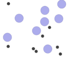
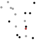
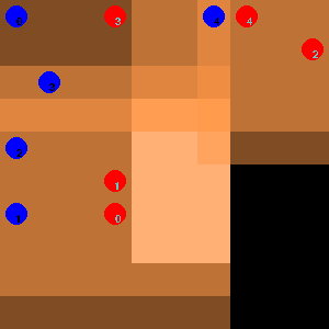
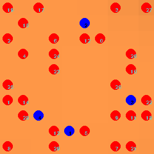
Our experiments are performed on three cooperative tasks: Pursuit, originally proposed in [17] and visualized in Figure 1, and, Simple-Spread and Simple-Push from multi-agent particle-world (MPE) [7] shown in Figure 2. These three environments are now both maintained by PettingZoo [33]. Note that the observation spaces in the original implementation of Simple-Spread and Simple-Push change when the number of agents changes. To address the change in the input dimension and to focus on the curriculum learning part, our agents observe only the closest four agents and landmarks resulting in partial observability.

Comparison: We compare SPMARL with (1) vanilla IPPO without curriculum learning, (2) IPPO with fine-grained linear curriculum learning (linear), which linearly increases the number of agents as well as other environment related factors. Although simple, the linear increasing paradigm represents existing methods since the methods usually scale the number of agents from few to more in a presumed manner as discussed in Section 3. Furthermore, we show the performance of a linearly decreasing number of agents, EPC (epc), and VACL in the Pursuit problem, even though EPC is orthogonal to our method as it uses linear scaling and VACL only controls the initial positions of the agents. For controlling the number of agents, VACL uses a linearly increasing order. The training details are described in Appendix A.

5.1 Pursuit

The Pursuit problem, also known as the Pursuit-Evasion problem, is a classic multi-agent task that represents a set of real-world tasks [34]. In this environment, ten agents are rewarded for catching ten evaders in a $30\times 30$ grid world with obstacles. To catch an evader more than two agents need to cooperatively surround the evader. At each time step each agent observes a $7\times 7$ image with three channels where each channel specifies the binary value of an existing agent, evader, or obstacle, respectively. In addition to controlling the number of agents and grid world size, in this task we also empirically study the outcomes with both the Sum and Average based optimization objectives. Note that in both cases using the Sum and Average, the evaluation is performed on the target task with fixed number of agents.

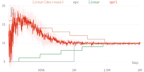
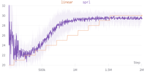
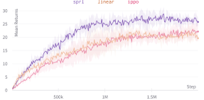
Sum: The results using Sum are reported in Figure 3. In the evaluation Figure 3(a), SPMARL outperforms the other baselines with considerable margins. Naive linearly increasing number of agents is not sufficient for high performance. For SPMARL, the number of agents shown in Figure 3(c) starts to grow quickly and then when the training performance in Figure 3(b) achieves some threshold, it goes down and converges to the target number $10$. linear (decrease) is inspired by the curriculum induced by SPMARL and is consistent with the idea that more agents make the Pursuit task easier. As expected, it improves the performance compared to vanilla IPPO but is outperformed by SPMARL’s more flexible curriculum. Figure 3(d) indicates the grid world size has a contrary process to the number of agents, going down and then up. This is consistent with the intuition in the pursuit task that it is easier to catch the evaders if there are more agents and a smaller grid world size.

(a) Evaluation

(b) Training

(c) Number of agents

(d) Grid world size

Figure 3: Learning process and contexts in pursuit generated by vanilla IPPO (ippo), IPPO with linear curricula (linear), IPPO with decreasing order (linear (decrease)), VACL with target distribution using uniform distribution (vacl (uniform)) and Gaussian distribution (vacl (gaussian)), EPC with linear increasing order (epc) and SPMARL (sprl) and its ablation variants (sprl (num), and sprl (grid)) when using a sum based global shared reward. Sub-figures (a) and (b) show the mean return for the comparison methods during evaluation on the target task and during training on the curriculum tasks (for IPPO the curriculum task is the target task), respectively. (c) and (d) show how the context variables that curriculum learning methods are controlling change during training, where (c) shows the number of agents and (d) grid world size. Each plot shows the mean of five algorithmic runs with shaded area denoting standard deviation.

Figure 4: Emergent number of agents as curricula, where sprl (num) is our method, vacl (uniform) and gaussian denote VACL using uniform distribution and a narrow Gaussian distribution as target distribution, respectively.

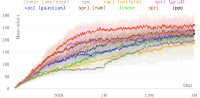
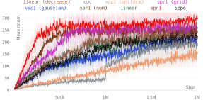
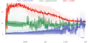
Ablation Study: In order to further investigate whether the number of agents can be an effective curriculum variable, we compare SPMARL only controlling the number of agents sprl (num) and only the grid world size sprl (grid) with the recent method VACL. As VACL originally only uses a uniform distribution vacl (uniform) as the target distribution which is not suitable for controlling the number of agents, we also conduct a variant vacl (gaussian) with a similar target distribution as used in SPMARL. Figure 3 shows that that both sprl (num) and sprl (grid) can still improve the performance and outperform vacl (uniform) and vacl (gaussian). One possible reason can be the emergent curricula in Figure 4, where sprl (num) generates more agents after early exploration ($\sim 100K$ steps), and maintains a higher number of agents for longer. In contrast, both vacl (gaussian) and vacl (uniform) move quickly to the target distribution without fully employing the easier tasks to boost the performance.

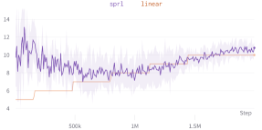
Average: Figure 5(a) shows that averaging the rewards over the number of agents degrades the effectiveness of using the number of agents as a curriculum. Although more agents can still catch evaders easier, averaging increased rewards over increased number of agents reduces the advantage of more agents which is shown in the curriculum created by SPMARL in Figure 5(c). Nonetheless, SPMARL can still take advantage of the other environment factor to create curricula as shown in Figure 5(d) and as was also shown for the Sum case in Figure 3(d). In both conditions reducing grid world size will help agents to obtain higher reward.

Discussion on Sum vs. Average: Using Sum rewards, the global reward is the sum of rewards due to captured evaders captured by all agents. For Average rewards, the global reward is averaged over all the agents. When the number of agents is fixed the Sum and Average rewards share the same optimal policy. However, when the number of agents changes and the number of evaders is fixed, the Average way implicitly imposes competition between agents and discourages more agents to cooperate. This is well demonstrated in Figure 5(c). This is an interesting observation that needs to be taken into account when choosing the reward function to be used with curriculum MARL.

(a) Evaluation

(b) Training

(c) Number of agents

(d) Grid world size

Figure 5: Learning process and contexts generated when using average to evaluate pursuit.

5.2 MPE Tasks

Simple-Spread: The target task in this environment is to control $8$ agents to cover $8$ landmarks. Agents are penalized by the sum of distances between each landmark and the closest agent. Original observation of each agent includes its velocity and all the other agents’ position as well as positions of all landmarks. In order to keep the observation dimension same when the number of agents changes and focus on the effect of curriculum learning, we adjust the environment to be partially observable, i.e., each agent only observes the closest $4$ agents and landmarks.

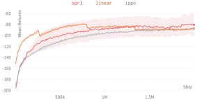
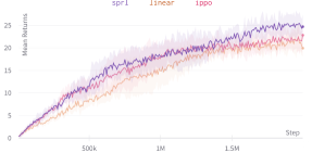
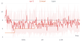
Evaluation performance is shown in Figure 6, while the training process is shown in Figure 9(b) in the Appendix C. Figure 6(b) does not show substantial impact of using the number of agents as a curriculum. We report the result as we hypothesize two possible reasons for this and hope they can inspire future research: (1) as the number of landmarks changes at the same pace with the number of agents, it is hard to distinguish the difficulty between different tasks, (2) as we generate more agents, agents collide more frequently, changing the dynamics of the task, which may make it harder to transfer from one context to another. The result also shows that the number of agents is potentially a complex curriculum variable since it may significantly influence the dynamics in some benchmarks.

(a) Evaluation

(b) Number of agents

Figure 6: The learning process on the benchmark of Simple-Spread.

Simple-Push: The Simple-Push task is originally an adversarial task in PettingZoo where we need to control the agents and an adversary at the same time. For a co-operative task, we set a random policy for the adversary. The agents have the same observation space as in Simple-Spread, but they cannot distinguish the adversary from cooperative agents, which increases the difficulty. In this task, we set a fixed number of landmarks. Intuitively, as with the Sum reward in Pursuit, a larger number of agents is expected to increase the total reward.

(a) Evaluation

(b) Number of agents

Figure 7: The learning process on the benchmark of Simple-Push.

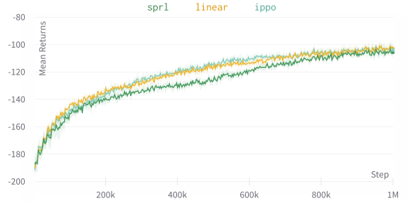
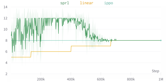
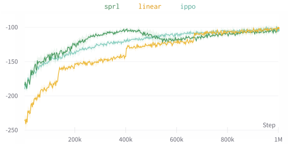
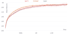
The learned curriculum over the number of agents in Figure 7(b) indicates that more agents should be able to cover all the $8$ landmarks easier. Nonetheless, using the results in Figure 7 we find that in both the Simple-Push and in the Simple-Spread tasks, all the three methods converge to similar performance. Note that this performance is sufficiently high compared to the data reported in [9]. For these methods, the effectiveness of the number of agents as a curriculum is not significant.

6 Discussion

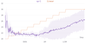
Curriculum learning works on the implicit assumption that the curricula used maintain continuation with the target task [12]. Therefore, as other environment or reward related factors, whether the number of agents is an effective curriculum variable depends on how it fundamentally changes the task, how smoothly it is connected to the target task, and the capacity of the underlying MARL algorithm. Our experiments show three different patterns: (1) In the Pursuit problem, the number of agents can well distinguish the difficulties of curricula and transfer to the next training stage. (2) In the Simple-Spread, since the agent size is large and collision between agents is allowed, even though more agents can help cover the landmarks, the collisions also happen more frequently and interfere with learning. This is confirmed by the learning process using linear increasing order as in Figure 9(a), where the performance drops when the number of agents increases. The drop, to some extent, can be attributed to the adaptability of the policy but it also indicates that the changed dynamics degrade the advantage of more agents. (3) In the Simple-Push environment, with a smaller number of agents than in Simple-Spread, collisions seldom happen. SPMARL is able to utilize more agents in the curriculum as shown in Figure 9(b). This is consistent with the linear case where the performance increases when increasing the number of agents. These different patterns show the adaptability of SPMARL and demonstrate the importance to further study the interaction between agents, environment dynamics and the characteristics of underlying MARL algorithms.

7 Conclusion

This paper presents a principled approach, self-paced multi-agent reinforcement learning (SPMARL), to generate curricula for MARL. Especially, when it is unclear how particular environment contexts or number of agents will influence the performance [35], SPMARL can automatically estimate the difficulty of curricula instances under any changing learned policies and design the curriculum sequence accordingly. We argue that naively assuming we should train MARL from few to more agents is not in general true. To our best knowledge, although limited to empirical study, this is the first work to investigate different ways to scale agents and propose a principled method to adaptively design the order of agents. With SPMARL, we empirically investigate how the number of agents can change to form effective curricula, show how the emergent numbers of agents reflect the dynamics change of the tasks in two different ways (Sum or Average), and demonstrate the effectiveness of SPMARL. We believe these initial results can be inspiring to motivate further theoretical research on how the tasks change w.r.t. number of agents and finally to provide a better way to scale agents.

Appendix A Training Details

A.1 IPPO Hyper-Parameters

The hyper-parameters used for IPPO are kept the same for all the experiments, as shown in Table 1. Note that these hyper-parameters are used to reproduce our results, but they can be fine tuned to further improve the performance. Each experiment can be run on computers with regular CPUs and one GPU with more than $2G$ memory, and it roughly takes one day to converge.

Table 1: Hyper-parameters for IPPO.

Hyper-parameters						Value
Actor layers						$3$
Actor learning rate						$0.0001$
Critic layers						$3$
Critic learning rate						$0.0001$
PPO update steps						$10000$
PPO update epochs						$80$
PPO clip						$0.2$
Discount rate						$0.99$

A.2 SPMARL Hyper-Parameters

The hyper-parameters used in our paramteters are shown in Table 2.

Table 2: Hyper-parameters for SPMARL.

Hyper-parameters	Pursuit	Simple-Spread	Simple-Push
Lower Context Bounds	$[20,3]$	$5$	$5$
Upper Context Bounds	$[40,20]$	$12$	$12$
Initial Mean	$[20,5]$	$9$	$9$
Initial Variance	$\begin{bmatrix}400&0\\ 0&225\end{bmatrix}$	$[16]$	$[16]$
Target Mean	$[30,10]$	$8$	$8$
Target Variance	$\begin{bmatrix}4e-3&0\\ 0&4e-3\end{bmatrix}$	$[4e-3]$	$[4e-3]$
Std Lower Bound	$[0.2,0.1]$	$[0.6]$	$[0.1]$
KL Threshold	$8000$	$8000$	$8000$
MAX KL	$0.05$	$0.05$	$0.05$

Appendix B Architectures Comparison

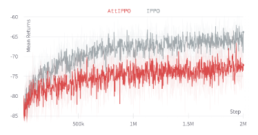
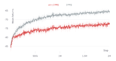
During our experiments, we compare the performance of fully connected neural network with attention based architecture [5]. The learning results are shown as Figure 8. As the attention based architecture is significantly outperformed by vinilla IPPO, in our formal experiments, we choose decide to adjust the environment to be partially observable in order to keep the dimension of observation space consistent when the number of agents varies. It should be note that even though the modified environment provides less information to our agents, the final performance is still promising, as shown in Figure 3(a) with $8$ agents IPPO achieves significant improvement during training. This is investigated and analyzed in prior work [22] which marks that counter-intuitively, the larger size of full state including information irrelevant to the task may adversely impact learning.

(a) Evaluation

(b) Training

Figure 8: Performance on fully-observable Simpe-Spread benchmark with $4$ agents using different architecture, where AttIPPO is the one using attention architecture, IPPO uses normal fully connected neural network.

Appendix C Training processes of MPE tasks

The training processes of Simple-Spread and Simple-Push are shown as Figure 9(a) and Figure 9(b), respectively.

(a) Simple-Spread

(b) Simple-Push

Figure 9: The training processes on MPE tasks.

References

- [1] Sutton, R. S., A. G. Barto. Reinforcement learning: An introduction. MIT press, 2018.
- [2] Hernandez-Leal, P., B. Kartal, M. E. Taylor. A survey and critique of multiagent deep reinforcement learning. Autonomous Agents and Multi-Agent Systems, 33(6):750–797, 2019.
- [3] Bengio, Y., J. Louradour, R. Collobert, et al. Curriculum learning. In Proceedings of the 26th annual international conference on machine learning, pages 41–48. 2009.
- [4] Wang, W., T. Yang, Y. Liu, et al. From few to more: Large-scale dynamic multiagent curriculum learning. In Proceedings of the AAAI Conference on Artificial Intelligence, vol. 34, pages 7293–7300. 2020.
- [5] Long, Q., Z. Zhou, A. Gupta, et al. Evolutionary population curriculum for scaling multi-agent reinforcement learning. arXiv preprint arXiv:2003.10423, 2020.
- [6] Chen, J., Y. Zhang, Y. Xu, et al. Variational automatic curriculum learning for sparse-reward cooperative multi-agent problems. Advances in Neural Information Processing Systems, 34, 2021.
- [7] Lowe, R., Y. Wu, A. Tamar, et al. Multi-agent actor-critic for mixed cooperative-competitive environments. arXiv preprint arXiv:1706.02275, 2017.
- [8] Rashid, T., M. Samvelyan, C. Schroeder, et al. Qmix: Monotonic value function factorisation for deep multi-agent reinforcement learning. In International Conference on Machine Learning, pages 4295–4304. PMLR, 2018.
- [9] Chao, Y., A. VELU, E. VINITSKY, et al. The surprising effectiveness of ppo in cooperative, multi-agent games. arXiv preprint arXiv:2103.01955, 2021.
- [10] Klink, P., H. Abdulsamad, B. Belousov, et al. A probabilistic interpretation of self-paced learning with applications to reinforcement learning. arXiv preprint arXiv:2102.13176, 2021.
- [11] Schaul, T., D. Horgan, K. Gregor, et al. Universal value function approximators. In International conference on machine learning, pages 1312–1320. PMLR, 2015.
- [12] Narvekar, S., B. Peng, M. Leonetti, et al. Curriculum learning for reinforcement learning domains: A framework and survey. arXiv preprint arXiv:2003.04960, 2020.
- [13] Portelas, R., C. Colas, L. Weng, et al. Automatic curriculum learning for deep rl: A short survey. arXiv preprint arXiv:2003.04664, 2020.
- [14] Oliehoek, F. A., C. Amato. A concise introduction to decentralized POMDPs. Springer, 2016.
- [15] Shapley, L. S. Stochastic games. Proceedings of the national academy of sciences, 39(10):1095–1100, 1953.
- [16] Littman, M. L. Markov games as a framework for multi-agent reinforcement learning. In Machine learning proceedings 1994, pages 157–163. Elsevier, 1994.
- [17] Gupta, J. K., M. Egorov, M. Kochenderfer. Cooperative multi-agent control using deep reinforcement learning. In International Conference on Autonomous Agents and Multiagent Systems, pages 66–83. Springer, 2017.
- [18] Claus, C., C. Boutilier. The dynamics of reinforcement learning in cooperative multiagent systems. AAAI/IAAI, 1998(746-752):2, 1998.
- [19] Sunehag, P., G. Lever, A. Gruslys, et al. Value-decomposition networks for cooperative multi-agent learning. arXiv preprint arXiv:1706.05296, 2017.
- [20] Foerster, J., G. Farquhar, T. Afouras, et al. Counterfactual multi-agent policy gradients. In Proceedings of the AAAI Conference on Artificial Intelligence, vol. 32. 2018.
- [21] Wei, E., S. Luke. Lenient learning in independent-learner stochastic cooperative games. The Journal of Machine Learning Research, 17(1):2914–2955, 2016.
- [22] de Witt, C. S., T. Gupta, D. Makoviichuk, et al. Is independent learning all you need in the starcraft multi-agent challenge? arXiv preprint arXiv:2011.09533, 2020.
- [23] Florensa, C., D. Held, X. Geng, et al. Automatic goal generation for reinforcement learning agents. In International conference on machine learning, pages 1515–1528. PMLR, 2018.
- [24] Racaniere, S., A. Lampinen, A. Santoro, et al. Automated curriculum generation through setter-solver interactions. In International Conference on Learning Representations. 2019.
- [25] Florensa, C., D. Held, M. Wulfmeier, et al. Reverse curriculum generation for reinforcement learning. In Conference on robot learning, pages 482–495. PMLR, 2017.
- [26] Klink, P., H. Abdulsamad, B. Belousov, et al. Self-paced contextual reinforcement learning. In Conference on Robot Learning, pages 513–529. PMLR, 2020.
- [27] Liu, Q., D. Wang. Stein variational gradient descent: A general purpose bayesian inference algorithm. arXiv preprint arXiv:1608.04471, 2016.
- [28] Virtanen, P., R. Gommers, T. E. Oliphant, et al. Scipy 1.0: fundamental algorithms for scientific computing in python. Nature methods, 17(3):261–272, 2020.
- [29] Peng, B., T. Rashid, C. A. S. de Witt, et al. Facmac: Factored multi-agent centralised policy gradients. arXiv preprint arXiv:2003.06709, 2020.
- [30] Terry, J. K., N. Grammel, A. Hari, et al. Revisiting parameter sharing in multi-agent deep reinforcement learning. arXiv preprint arXiv:2005.13625, 2020.
- [31] Tan, M. Multi-agent reinforcement learning: Independent vs. cooperative agents. In Proceedings of the tenth international conference on machine learning, pages 330–337. 1993.
- [32] Schulman, J., F. Wolski, P. Dhariwal, et al. Proximal policy optimization algorithms. arXiv preprint arXiv:1707.06347, 2017.
- [33] Terry, J. K., B. Black, M. Jayakumar, et al. Pettingzoo: Gym for multi-agent reinforcement learning. arXiv preprint arXiv:2009.14471, 2020.
- [34] de Souza, C., R. Newbury, A. Cosgun, et al. Decentralized multi-agent pursuit using deep reinforcement learning. IEEE Robotics and Automation Letters, 6(3):4552–4559, 2021.
- [35] Co-Reyes, J. D., S. Sanjeev, G. Berseth, et al. Ecological reinforcement learning. arXiv preprint arXiv:2006.12478, 2020.