Conformal Prediction with Temporal Quantile Adjustments

Abstract

We develop Temporal Quantile Adjustment (TQA), a general method to construct efficient and valid prediction intervals (PIs) for regression on cross-sectional time series data. Such data is common in many domains, including econometrics and healthcare. A canonical example in healthcare is predicting patient outcomes using physiological time-series data, where a population of patients composes a cross-section. Reliable PI estimators in this setting must address two distinct notions of coverage: cross-sectional coverage across a cross-sectional slice, and longitudinal coverage along the temporal dimension for each time series. Recent works have explored adapting Conformal Prediction (CP) to obtain PIs in the time series context. However, none handles both notions of coverage simultaneously. CP methods typically query a pre-specified quantile from the distribution of nonconformity scores on a calibration set. TQA adjusts the quantile to query in CP at each time $t$, accounting for both cross-sectional and longitudinal coverage in a theoretically-grounded manner. The post-hoc nature of TQA facilitates its use as a general wrapper around any time series regression model. We validate TQA’s performance through extensive experimentation: TQA generally obtains efficient PIs and improves longitudinal coverage while preserving cross-sectional coverage.

1 Introduction

The impressive predictive performance of modern “black-box” machine learning methods has started to make them critical ingredients in various high-stakes decision-making pipelines. It is thus increasingly important to quantify the predictive uncertainty of such models reliably and efficiently, which remains a fundamental challenge. Conformal Prediction (CP), pioneered by Vovk et al. [50], is a powerful framework for quantifying uncertainty under mild assumptions. The model-agnostic and distribution-free nature of CP makes it particularly suitable for large neural network models, and has started to attract the attention of the deep learning community [2, 3, 6, 9, 31, 56]. The primary assumption in most current CP methods is that of data exchangeability. For instance, only assuming exchangeability of the calibration and test data, one can construct $1-\alpha$ valid prediction intervals by simply querying the corresponding quantile of nonconformity scores on the calibration set. Recent works have started exploring the adaptation of CP in settings that go beyond the usual exchangeability assumption [4, 15, 19, 35, 39, 40, 41, 47, 54], and to more complex data such as time series [15, 45, 53, 55].

We study the adaptation of CP to the cross-sectional time series regression setting. More formally, suppose our data comprises of $N$ time series, denoted $\{\mathbf{S}_{i}\}_{i=1}^{N}$, with each $\mathbf{S}_{i}$ sampled from an arbitrary distribution $\mathcal{P}_{S}$. Further, each time series $\mathbf{S}_{i}$ is a sequence of temporally-dependent random variables $[Z_{i,1}\ldots,Z_{i,t},\ldots,Z_{i,T}]$ , with $Z_{i,t}=(X_{i,t}Y_{i,t})$ consisting of covariates $X_{\cdot,\cdot}\in\mathbb{R}^{d}$ and the response $Y_{\cdot,\cdot}\in\mathbb{R}$. Given data $\{Z_{N+1,j}\}_{j=1}^{t}$ until time $t$ for a new time series $\mathbf{S}_{N+1}$, the time series regression problem entails predicting the response $Y_{N+1,t+1}$ at (unknown) time $t+1$. We are interested in quantifying the uncertainty of each prediction by constructing valid prediction intervals (PI). That is, given a confidence level $1-\alpha$, we are interested in constructing a prediction interval, $\hat{C}_{\alpha,N+1,t+1}$, that will cover $Y_{N+1,t+1}$ with probability of at least $1-\alpha$.

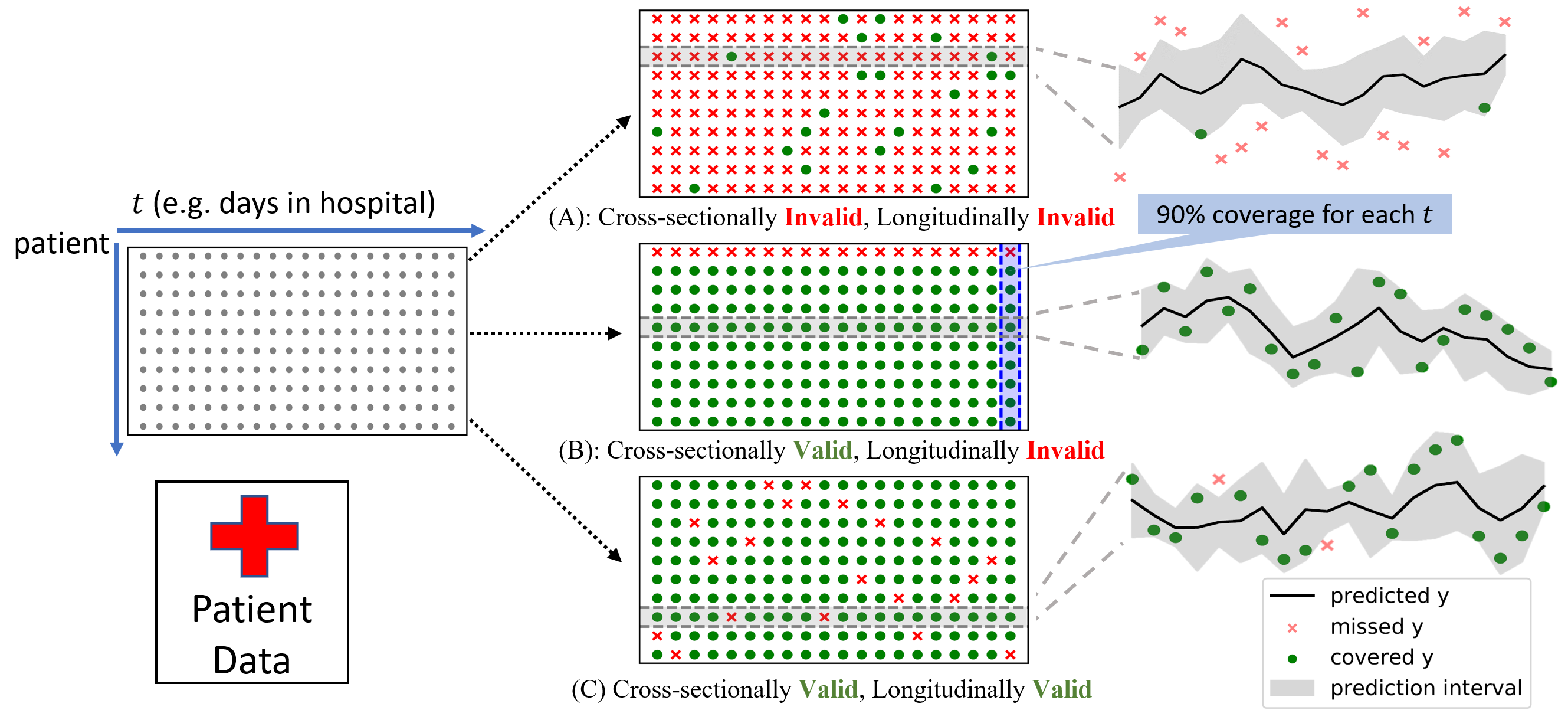
A crucial requirement in cross-sectional time series regression is to distinguish two notions of validity, longitudinal and cross-sectional, to ensure reliable performance. Longitudinal validity is concerned with validity along the temporal axis for each time series. On the other hand, cross-sectional validity is concerned with validity across the populational cross-section of the time series data. Figure 1 illustrates both notions of validity and a standard real-world occurrence of such a problem setting. Recently, several research groups have explored adapting CP to the time series setting. Some of this work [15, 55, 53] focuses only on longitudinal validity, which is extremely difficult without strong distributional assumptions [4]. Furthermore, such methods cannot leverage rich information inherent in the cross-section. The only work which addresses cross-sectional validity is to due to Stankevičiūtė et al. [45], but it ignores the temporal dependence. Accounting for both notions of coverage is critical to obtain reliable performance.

To remedy the above situation, we propose Temporal Quantile Adjustment (TQA) for CP in the cross-sectional time series regression setting. TQA is the first method that can account for both cross-sectional and longitudinal validity simultaneously. Although TQA can be used as a wrapper around any time series regression model, we focus on neural networks, as our main inspiration comes from complicated time series regression problems in healthcare. Neural networks are particularly suited for such tasks, which can involve modeling the evolution of heterogeneous entities such as diagnostic and drug codes, patient and physician embeddings and regressing over a target of interest. Taking inspiration from [15], TQA adjusts the quantile to query at each time step in a theoretically-grounded manner. Based on the nature of quantile adjustment, we also propose two variants of TQA, which further shed light on the generality of our method. The ability of TQA to handle both cross-sectional and longitudinal validity is borne out in extensive experimentation, where it significantly outperforms competing methods.

Figure 1: PI estimators with different cross-sectional or longitudinal properties/validities. × denotes the ground-truth $y$ that is outside of the PI. (A) features PIs that are not valid in either sense: $Y$ is never covered. (B) is cross-sectionally valid: for any $t$, 90% of the $Y_{\cdot,t}$ are covered. It is longitudinally invalid, as 10% of the TS receive no coverage at all. (C) exhibits both cross-sectional and longitudinal validity, which is ideal.

2 Related Work

Our work falls squarely within the Conformal Prediction (CP) framework. The original formulation of CP was in a purely transductive setting [43, 44, 50], and was computationally inefficient. More efficient variants dubbed as Inductive Conformal Prediction (ICP) [36, 37, 49] were proposed soon after and were more broadly popularized by followup works in statistics [27, 29, 30]. A similar idea, often referred to as Split Conformal [28], is now more or less used interchangeably with ICP, and is fundamental to our paper. The model-agnostic and distribution-free nature of split conformal makes it suitable for large black-box models, and thus it has seen adoption in deep learning-based pipelines (e.g. [2, 11, 24, 31, 33, 45]).

One of the mainstays of the CP framework is the assumption of exchangeability between calibration and test data. Extensions of CP “beyond exchangeability” have attracted relatively little attention until recently. A key publication in the area is [47] which used the notion of weighted exchangeability to handle covariate shift. Several notable works that address various aspects of the covariate shift problem include [19, 39, 54, 41]. More recent work [4, 15] handles gradual distribution drifts. [4] additionally proposes an extension of CP when the data-points cannot be treated in a symmetric manner. Extensions of the split conformal method to a broad class of dependent processes such as stationary $\beta$-mixing processes was proposed by [35]. These works provide some general methodological insights to model temporal dependence in our case, but are otherwise not directly related. In particular, the online adaptive method of [15], served as a major source of inspiration for the development of a variant of TQA (dubbed TQA-E). The most related works have a focus on generating valid intervals in time series regression [15, 55, 4, 53]. These works end up ignoring cross-sectional aspects, which is understandable given the tasks they study. On the other extreme is [45], which focuses only on cross-sectional coverage, ignoring the temporal dimension in constructing PIs.

Various other techniques, outside the ambit of CP, have also been extended to quantify uncertainty in time series forecasting as well. For instance, approximate Bayesian methods [8, 51, 34, 32, 23, 13, 26] are quite popular for uncertainty quantification, and have been extended to RNNs [12, 7]. Finally, one may also use the idea of directly predicting the quantiles (as opposed to the point estimate) in regression tasks [46, 25], and applying it to time series forecasting [52, 14]. However, such methods usually require changing the base model and typically do not come with coverage guarantees.

3 Preliminaries

This section builds foundation for our exposition of TQA. We begin by expounding further on longitudinal and cross-sectional validity, followed by presenting the exchangeability assumption. Finally, we discuss the use of split conformal prediction to construct (cross-sectionally) valid PIs.

3.1 Cross-sectional Validity vs Longitudinal Validity

Cross-sectional validity is the more common type of validity encountered in CP, being the only type of validity in non-time-series settings. More formally:

Definition 1.

Prediction interval $\hat{C}_{\cdot,\cdot}$ is $1-\alpha$ cross-sectionally valid if, for any $t$,

$$\mathbb{P}_{\mathbf{S}_{N+1}}\{Y_{N+1,t}\in\hat{C}_{N+1,t}\}\geq 1-\alpha.$$ (1)

$\mathbb{P}_{\mathbf{S}_{N+1}}$ means the probability is taken over the randomness of $\mathbf{S}_{N+1}$. If $\hat{C}_{N+1,t}$ is random (e.g. depends on $\{\mathbf{S}_{i}\}_{i=1}^{N}$) then the probability is taken over the randomness of $\hat{C}_{N+1,t}$ as well. Note that if we consider the case where every time series only consists of one step ($T=1$), then we recover the usual definition of marginal validity. Cross-sectional validity translates to high-probability in coverage for a randomly drawn time series. As we will see later, cross-sectional validity is easier to achieve, since we can assume inter-time-series exchangeability.

Longitudinal validity, on the other hand, is concerned with coverage along the temporal axis for a particular TS. We use the following definition:

Definition 2.

Prediction interval $\hat{C}_{\cdot,\cdot}$ is $1-\alpha$ longitudinally valid if for almost every time-series $\mathbf{S}_{N+1}\sim\mathcal{P}_{S}$ there exists a $T_{0}$ such that:

$$t>T_{0}\implies\mathbb{P}_{Y_{N+1,t}|\mathbf{S}_{N+1,:t-1}}\{Y_{N+1,t}\in\hat{C}_{N+1,t}\}\geq 1-\alpha.$$ (2)

Here, the qualifier “almost every” means that the set of time series’ for which such coverage may fail is of measure zero (under $\mathcal{P}_{S}$). The threshold $T_{0}$ allows some “time” for $\hat{C}$ to potentially adapt to the temporal information in a particular TS. It should be clear that longitudinal validity is harder to attain, because we can no longer marginalize the probability over randomly drawn time series.

3.2 Conformal Prediction for Cross-sectionally Valid PI

In this section we explain how to use conformal prediction to construct cross-sectionally valid PIs. We first introduce exchangeability assumption, which is the central assumption in conformal prediction, and slightly weaker than the standard i.i.d assumption. More formally:

Definition 3.

(Exchangeability [50]) A sequence of random variables, $Z_{1},Z_{2},\ldots,Z_{n}\in\mathcal{Z}$ are exchangeable if for any permutation $\pi:\{1,2,\dots,n\}\to\{1,2,\dots,n\}$, and every measurable set $E\subseteq\mathcal{Z}^{n}$, we have

$$\mathbb{P}\{(Z_{1},Z_{2},\ldots,Z_{n})\in E\}=\mathbb{P}\{(Z_{\pi(1)},Z_{\pi(2)},\ldots,Z_{\pi(n)})\in E\}$$ (3)

Definition 3 can naturally be extended to a sequence of randomly drawn time series:

Definition 4.

(Exchangeable Time Series) Given time series $\mathbf{S}_{1},\mathbf{S}_{2},\ldots,\mathbf{S}_{n}$ where $\mathbf{S}_{i}=[Z_{i,1},\ldots,Z_{i,T},\ldots]$, denote $Z_{i,\{t_{j}\}_{j=1}^{m}}$ as the concatenated random variable of $(Z_{i,t_{1}},\ldots,Z_{i,t_{m}})$. Time series $\mathbf{S}_{1},\mathbf{S}_{2},\ldots,\mathbf{S}_{n}$ are exchangeable if, for any finitely many $t_{1}<\cdots<t_{m}$, the random variables $Z_{1,\{t_{j}\}_{j=1}^{m}},\ldots,Z_{n,\{t_{j}\}_{j=1}^{m}}$ are exchangeable.

As a concrete example, suppose we randomly pick 100 patients from a hospital’s EHR database for predicting readmission risk. It is fairly reasonable to assume that these time series are exchangeable, despite the obvious strong temporal dependence within each time series. Throughout this paper, we will assume $\mathbf{S}_{1},\ldots,\mathbf{S}_{N+1}$ are exchangeable time series.

We now explain how to construct cross-sectionally valid PIs. To construct a PI for $Y_{i,t}$, we first split our training data $\{\mathbf{S}_{i}\}_{i=1}^{N}$ into a proper training set and a calibration set [38]. The training set is used to train models for the nonconformity score function, and the calibration set is used to collect such nonconformity scores (denoted as $V(\cdot)$). For example, one may train a mean estimator $\hat{\mu}$ (e.g. an RNN) on the training set, and use the absolute residual $v_{i,t}\leftarrow|y_{i,t}-\hat{y}_{i,t}|$, where $\hat{y}_{i,t}=\hat{\mu}(X_{i,t};\mathbf{S}_{i,:t-1})$, as the nonconformity score. Here $\mathbf{S}_{i,:t-1}$ denotes $[Z_{i,1},\ldots,Z_{i,t-1}]$. The idea behind the split conformal method is that the scoring function (e.g. $\hat{\mu}$) is only fit on the proper training set, implying that nonconformity scores on the calibration set and $v_{N+1,t}$ are also exchangeable. Here on, for the sake of simplicity of notation, we will use $\{\mathbf{S}_{i}\}_{i=1}^{N}$ to denote the calibration set only, assuming all necessary models have already been trained.

Given a nonconformity score $V(\cdot)$ (possibly using some trained model $\hat{\mu}$) and a set of exchangeable time series $\{\mathbf{S}_{i}\}_{i=1}^{N+1}$, the split conformal method can be used to generate the following $1-\alpha$ cross-sectionally valid prediction interval:

$$\hat{C}^{split}_{N+1,t+1}=\Bigg{\{}y:V_{N+1,t+1}(\hat{y},y)\leq Q\Big{(}1-\alpha;\{v_{j,t+1}\}_{j=1}^{N}\cup\{V_{N+1,t+1}(\hat{y},y)\}\Big{)}\Bigg{\}}.$$ (4)

Here, $Q(\beta;A)$ means the $\beta$-quantile for the set $A$. As a concrete example, if we let $v_{i,t}=|y_{i,t}-\hat{y}_{i,t}|$, and employ the standard trick that replaces $v_{N+1,t+1}$ with $\infty$ to avoid plugging in (uncountably) many values for $y$ [4], the prediction interval for $Y_{N+1,t+1}$ becomes:

$$\hat{C}^{split}_{N+1,t+1} \vcentcolon=[\hat{y}-\hat{v},\hat{y}+\hat{v}]\text{ where }\hat{v}\vcentcolon=Q\Big{(}1-\alpha;\{|y_{i,t+1}-\hat{y}_{i,t+1}|\}_{i=1}^{N}\cup\{\infty\}\}\Big{)}$$ (5)

Assuming exchangeability, we can easily show the cross-sectional validity of $\hat{C}^{split}$:

Theorem 3.1.

([4, 50]) $\hat{C}^{split}$ is $1-\alpha$ cross-sectionally valid (Def. 1).

The intuition behind the proof is that the exchangeability of the time series translates to the exchangeability of the nonconformity scores, which means the rank of $v_{N+1,t+1}$ among $\{v_{i,t+1}\}_{i=1}^{N+1}$ follows a uniform distribution. The coverage guarantee in Theorem 3.1 then follows. Note that with a finite calibration set, the $1-\alpha$-quantile could be ambiguously defined, and in practice one would use $\frac{\lceil(1-\alpha)(N+1)\rceil}{N+1}$ to get a slightly more conservative PI, or “flip a (biased) coin” to choose between $\frac{\lceil(1-\alpha)(N+1)\rceil}{N+1}$ and $\frac{\lfloor(1-\alpha)(N+1)\rfloor}{N+1}$ for a precise $1-\alpha$ coverage (e.g. the “smoothed” ICP in [50] or the tie-breaking trick in [2]). In Section 4, we assume the precise coverage PI for the ease of discussion.

While cross-sectionally valid, $\hat{C}^{split}$ ignores the temporal dependence in the nonconformity scores completely. We will explain in Section 4 how to adapt to the temporal dependence by “quantile adjustment”, thus improving longitudinal coverage as well.

4 Temporal Quantile Adjustment (TQA)

In Section 3 we discussed a classical conformal prediction method and also highlighted its inherent limitations in the time series setting. In this section we will formally introduce Temporal Quantile Adjustment (TQA), which queries quantiles differently than in the aforementioned split conformal procedures. We first explicate the goals and motivations of TQA in Section 4.1. Then, in Section 4.2 and 4.3 we propose two principled adjustment methods along with theoretical analyses.

4.1 Improving Longitudinal Coverage

Although it is tempting to directly pursue distribution-free finite-sample PI estimator that achieves longitudinal coverage guarantee (Def. 2), it is likely too optimistic due to the fact that $[Z_{i,1},\ldots,Z_{i,T}]$ are not exchangeable and we cannot characterize them meaningfully without imposing (strong) distributional assumptions. For example, in [4], the bound for coverage gap—which captures the loss in coverage compared to what is achievable under exchangeability—essentially becomes 1 as the data becomes time-dependent. In fact, one could view Def. 2 as a “conditional validity” (where $\mathbf{S}_{N+1,:t}$ as a whole is viewed as the input), and it is well-known that distribution-free finite-sample conditional validity is impossible to achieve in a meaningful way [5, 30].

Nevertheless, longitudinal coverage may still be empirically improved if we can adapt to the temporal dependence. From our EHR example, suppose $\hat{\mu}$ has been giving high-error predictions for a patient for 8 out of the past 10 days, we might suspect high error going forward for this patient as well. If this is indeed the case, then naively applying $\hat{C}^{split}$ can only attain low coverage for this patient, no matter how long a history we observe. To address this, we propose to query different quantiles based on the partially observed time series.

From now on, we use $\hat{C}_{a_{i,t},i,t}$ to denote a PI for $Y_{i,t}$ with a pre-specified target coverage of $1-a_{i,t}$, in order to emphasize dependence on the “quantile to query”. We let $a_{i,t}=\alpha-\hat{\delta}_{i,t}$, where $\hat{\delta}_{i,t}$ is the quantile adjustment. Classical split conformal PIs (e.g. [45]) entail a special case: $\forall i,\forall t,\hat{\delta}_{i,t}\equiv 0$. We refer to this method as Temporal Quantile Adjustment (TQA).

Now, denote the random variable $R_{i,t}$ as the rank/quantile of $V_{i,t}$ among $\{V_{j,t}\}_{j=1}^{N+1}$:

$$r_{i,t}\vcentcolon=Q^{-1}(v_{i,t};\{v_{j,t}\}_{j=1}^{N+1})\vcentcolon=\frac{|\{j:v_{j,t}<v_{i,t}\}|}{N+1}.$$ (6)

For example, if $v_{i,t}$ is the smallest among $\{v_{j,t}\}_{j=1}^{N+1}$, then $r_{i,t}=0$. Intuitively, we would like to use a more conservative (smaller) $a_{N+1,t}$ when we believe $\mathbf{S}_{N+1}$ as a whole is less “conformal” and $R_{N+1,t}$ is likely high. A crucial observation is that if there is no actual temporal dependence between the nonconformity scores (i.e. we are just adjusting $a_{t}$ based on some “noise”), then we do not lose any coverage as long as the expected adjustment is zero.

Theorem 4.1.

If the nonconformity score’s rank $(R_{N+1,t})$ is independent of the quantile adjustment $(\hat{\delta}_{N+1,t})$, then $\mathbb{P}_{\mathbf{S}_{N+1}}\{Y_{N+1,t}\in\hat{C}_{a_{N+1,t},N+1,t}\}\geq 1-\alpha+\mathbb{E}[\hat{\delta}_{N+1,t}]$.

All proofs are deferred to the Appendix.

Remark: The assumption in Theorem 4.1 is not that $\mathbf{S}_{N+1}$ itself is not temporally dependent, nor is it the slightly weaker assumption, that of the temporal independence of either $\{R_{\cdot,t}\}_{t=1}^{T}$ or $\{V_{\cdot,t}\}_{t=1}^{T}$. The assumption in Theorem 4.1 only suggests that there is no temporal pattern in the prediction errors that $\hat{\delta}$ can capture. This could happen, for example, when the RNN captures the underlying data generating process fully, but only misses the random noise (aleatoric uncertainty). This could also happen if our quantile adjustments $(\hat{\delta})$ are pure noise.

Unfortunately, although it can be tempting to conclude that $\mathbb{E}[\hat{\delta}_{N+1,t}]=0$ implies finite-sample cross-sectional validity, this conclusion would be incorrect, because it ignores the dependence between $\mathbf{1}\{Y_{N+1,t}\in\hat{C}_{a_{N+1,t},N+1,t}\}$ and $a_{N+1,t}$. However, we will next discuss how to perform quantile adjustment, and why it typically improves coverage.

4.2 Quantile Budgeting (TQA-B)

Figure 2: Coverage profiles with hypothetical realized rank $r$ condition on prediction $\hat{r}$, with $\alpha=0.2$ for readability. ($Y_{i,t}\in\hat{C}_{i,t}\Leftrightarrow r_{i,t}\leq 1-a_{i,t}$.) As $\hat{r}$ follows a uniform distribution, the proportion of dots below the red line represents the cross-sectional coverage probability. TQA-B generally improves coverage if $\hat{r}$ is correlated with the realized $r$ (middle), and does not lose coverage otherwise (right). “Budgeting” refers the constraint that sacrificed and gained have equal areas.

Theorem 4.1 provides an interesting constraint that we should consider while designing $\hat{\delta}$. That is, we should let $\mathbb{E}[\hat{\delta}]=0$ so as to keep the same coverage when we cannot predict the quantiles, but hopefully improving coverage when we can. This suggests a design of $\hat{\delta}$ that we refer to as a type of “budgeting”. Although it is possible to directly predict a good $\hat{\delta}_{i,t+1}$, we adopt a more principled two-step approach:

1. We predict quantile $\hat{r}_{i,t+1}$ which estimates $r_{i,t+1}$.

2. We use a pre-defined mapping $g$ to define the quantile adjustment $\hat{\delta}_{i,t+1}\leftarrow g(\hat{r}_{i,t+1};\alpha)$.

This also permits research to improve each component independently. We introduce one alternative for each step in the Appendix.

(i) Quantile Prediction: The quantile prediction $\hat{r}_{i,t+1}$ is estimated by a function of the form $f(\mathbf{S}_{i,:t};\{\mathbf{S}_{j,:t}\}_{j=1}^{N+1})$. Since $\hat{r}_{i,t+1}$ is supposed to predict $r_{i,t+1}$, the rank of the nonconformity score, we impose the constraint that $\hat{r}_{i,t+1}$ should follow a uniform distribution over $\{\frac{j}{N}\}_{j=0}^{N}$. We will focus on a simple rank prediction method stated below:

$$\hat{r}^{ms}_{i,t+1}\vcentcolon=Q^{-1}(\overline{\epsilon}_{i,t};\{\overline{\epsilon}_{j,t}\}_{j=1}^{N+1}) \text{ where }\overline{\epsilon}_{i,t}\vcentcolon=\sum_{t^{\prime}=1}^{t}\frac{|y_{i,t^{\prime}}-\hat{y}_{i,t^{\prime}}|}{t}\beta^{(t-t^{\prime})}.$$ (7)

Here, $\overline{\epsilon}_{i,t}$ is the exponentially decayed mean residual of time series $i$ up to time $t$, and we use $\beta=0.8$. Note that taking the rank with $Q^{-1}$ achieves the uniformity requirement, and $\overline{\epsilon}_{\cdot,t}$ could be replaced by any scoring function that takes into account the temporal information.

(ii) Budgeting: Given prediction $\hat{r}_{i,t}$, we propose the following adjustment $\hat{\delta}_{i,t}\vcentcolon=g^{B}(\hat{r}_{i,t};\alpha)$:

$$g^{B}(r;\alpha)\vcentcolon=\begin{cases}C(r-(1-\alpha))&(r<1-\alpha)\\ (r-(1-\alpha))&(r\geq 1-\alpha)\\ \end{cases}\text{ where }C=\frac{(2\alpha N-\lfloor\alpha N\rfloor)(\lfloor\alpha N\rfloor+1)}{\lceil(1-\alpha)N\rceil((1-2\alpha)N+1+\lfloor\alpha N\rfloor)}.$$ (8)

The particular coefficient design used ensures that the following property holds:

Theorem 4.2.

Using $\hat{r}^{ms}_{\cdot,\cdot}$ and $g^{B}$, $\forall t,\mathbb{E}_{\mathbf{S}_{N+1}}[a^{TQA-B}_{N+1,t}]=\alpha$.

Thus, by Theorem 4.1, TQA-B will not lose coverage if $\hat{r}$ and $r$ are independent. The following theorem provides a worst-case cross-sectional coverage guarantee, regardless of how “bad” $\hat{r}$ is:

Theorem 4.3.

$\mathbb{P}_{\mathbf{S}_{N+1}\sim\mathcal{P}_{S}}\{Y_{N+1,t+1}\in\hat{C}^{TQA-B}_{\alpha,N+1,t+1}\}\geq 1-\alpha-\underbrace{\Big{(}\frac{\alpha+\frac{1}{2N}}{1-\alpha+\frac{1}{2N}}\Big{)}^{2}(1-\alpha)}_{\text{worst-case loss}}.$

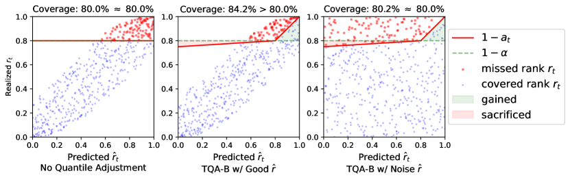
The worst-case loss term is typically small: about $0.012$ for $\alpha=0.1$ and $N=100$, although it can also be also be high for a large $\alpha$ like $0.5$. In practice, it is unlikely that $\hat{r}$ is worse than a random guess; the coverage is typically greater than $1-\alpha$, as we will see in the experiments and illustrated in Figure 2. In the Appendix, we present a more aggressive quantile adjustment function $g$ that provides a weaker guarantee than Theorem 4.3, but empirically performs better.

Implementation Details To avoid creating infinitely-wide PIs, we could also let $\hat{\delta}=\lambda g(\hat{r};\alpha)$ so $a_{t}$ is bounded away from 0 (In our experiments we choose $\lambda$ such that $a_{t}\geq 0.01$). Moreover, the specific form of $C$ presented in this section depends on the concrete distribution of $\hat{r}$. For example, $C$ would take a different form if $\hat{r}$ is defined to be uniform over $\{\frac{j}{N+1}\}_{j=1}^{N+1}$ rather than $\{\frac{j}{N}\}_{j=0}^{N}$. Practically, we can simply let $C=\alpha^{2}(1-\alpha)^{-2}$ regardless of $N$. The additional loss in Theorem 4.3 will become $\alpha^{2}/(1-\alpha)$, and the change in Theorem 4.2 is negligible for a reasonable value of $N$.

4.3 Error-based adjustment (TQA-E)

Another simple quantile adjustment approach is using a heuristic that depends on the past “errors”: Define $err_{t}=\mathbf{1}\{Y_{t}\not\in\hat{C}_{a_{t}}\}$, and increase $\delta_{t+1}$ (conservative) if we see too many errors in $\{err_{t^{\prime}}\}_{t^{\prime}<t+1}$ compared with $\alpha$, and vice versa. Since this approach does not depend on the cross-section, we drop the subscript $\cdot_{N+1}$ for simplicity. We use the following update rule (with $\hat{\delta}_{0}=0$) inspired by [15]:

$$\hat{\delta}_{t+1}\leftarrow\begin{cases}\hat{\delta}_{t}+\gamma(err_{t}-\alpha)&(\hat{\delta}_{t}\geq\alpha-1)\\ (1-\gamma)\hat{\delta}_{t}&(otherwise)\end{cases}.$$ (9)

Note that we do not explicitly impose the restriction that $\alpha-\hat{\delta}_{t}=a_{t}\in[0,1]$, which means the PI could have infinite width. However, infinite-wide PI means no error, so $\hat{\delta}_{t+1}$ will decrease and we resume to a finite PI gradually.

As $\hat{\delta}_{t}$ depends on the entire error history, it is not immediately clear whether TQA-E is still valid with the assumption in Theorem 4.1. Below we state a “no-worse” type theorem for TQA-E:

Theorem 4.4.

If we assume the nonconformity score’s rank has no temporal dependence, then

$$\forall t,\mathbb{E}_{\mathbf{S}_{N+1}\sim\mathcal{P}_{S}}[a^{TQA-E}_{N+1,t}]\leq\alpha.$$ (10)

Thus, $\hat{C}^{TQA-E}$ is finite-sample cross-sectional $1-\alpha$ valid following Theorem 4.1.

Finally, an asymptotic longitudinal validity result can also be shown for long time series:

Theorem 4.5.

(Asymptotic Longitudinal Coverage) For any time series $\mathbf{S}$, $\lim_{T\to\infty}\frac{\sum_{t=0}^{T-1}err_{t}}{T}\leq\alpha$.

Remarks: Although Theorem 4.5 seems to suggest some sort of longitudinal validity, it does not contradict the hardness claim in Section 4.1, because TQA-E achieves this via infinitely-wide PIs. We also refer interested readers to [55] as an example of an different heuristic based on errors of a single time series. However, it will require further modifications for finite-sample cross-sectional validity.

5 Experiments

In this section, our goal is to to verify the following empirically:

1. TQA maintains cross-sectional coverage and achieves competitive PI efficiency.

2. Ignoring temporal dependence in naive split conformal prediction leads to low longitudinal coverage for some TS.

3. TQA improves longitudinal coverage.

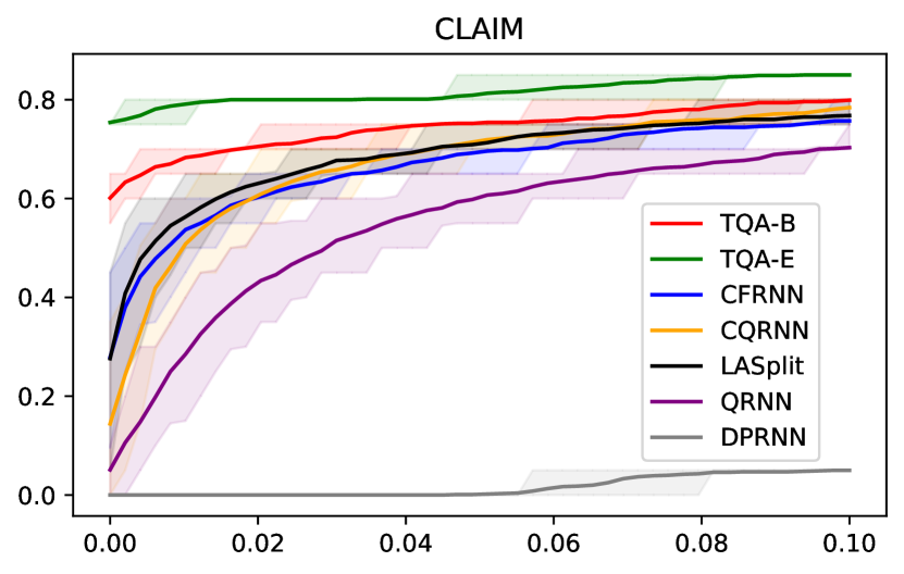
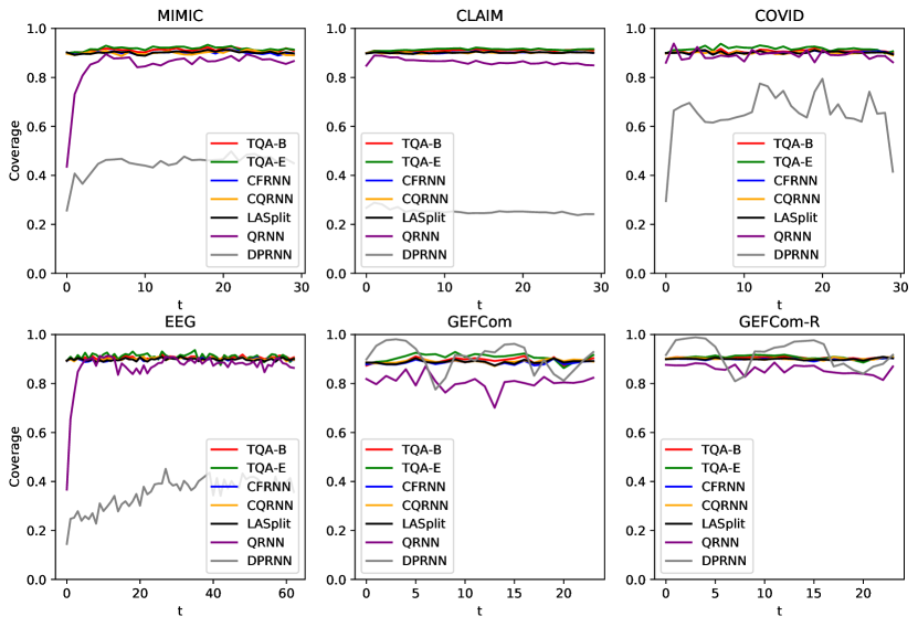
Baselines: We use the following state-of-the-art baselines for PI construction: Conformal forecasting RNN (CFRNN (Split)) [45]), a direct application of split-conformal prediction [50]; Quantile RNN (QRNN) [52], which directly predicts the two endpoints (represented by two quantiles) of the PI; RNN with Monte-Carlo Dropout (DP-RNN) [13]; Conformalized Quantile Regression with QRNN (CQRNN) [42], which, as the name suggests is a conformalized version of quantile regression; Locally adaptive split conformal prediction (LASplit) [27], which uses a normalized absolute error as the nonconformity score (we follow the implementation in [42]).

Table 1: Number of TSs in each dataset along with the length.

Properties	MIMIC	CLAIM	COVID	EEG	GEFCom/GEFCom-R
# train/cal/test	192/100/100	2393/500/500	200/100/80	300/100/200	1198/200/700
$T$ (length)	30	30	30	63	24

Figure 3: Coverage rate (Y-axis) vs the percentile among all test TS (X-axis, with zero meaning the least-covered TS) for the 10% least-covered TS in CLAIM. The bands denote the center 80% realizations. TQA-E has an natural advantage by using infinitely-wide PIs. However, even TQA-B still significantly improves the longitudinal coverage rate over all baselines.

Figure 4: Sorted absolute residuals ($|y-\hat{y}|$) for $t=T-10$. Each dataset is normalized so the mean of the residuals is 1. To cover extreme values, even if allowed to “sacrifice” some less extreme values, the PI on average is expected to get much wider. It is thus surprising that TQA-B could improve both efficiency and the tail coverage.

Datasets We test our methods and baselines on the following datasets: Electronic health records data for white blood cell counts (WBCC) prediction (MIMIC [21, 16, 20]), COVID-19 cases prediction (COVID [10]), Electroencephalography trajectory prediction after visual stimuli (EEG [48]), energy load forecasting (GEFCom [18]), and healthcare claim amount prediction (CLAIM) using data from a large American healthcare data provider. Among these, we mostly follow [45] in preparing MIMIC, COVID and EEG. Note that GEFCom is originally a single time series (hourly observations for years). Therefore, we treat each day as a single TS, and perform a strict temporal splitting (test data is preceded by calibration data, which is preceded by the training data), which means exchangeability is broken. We also include a GEFCom-R (andom) version that preserves the exchangeability by ignoring the temporal order in data splitting. Table 5 provides a brief summary of the data. Due to space constraints, the details for each dataset are relegated to the Appendix.

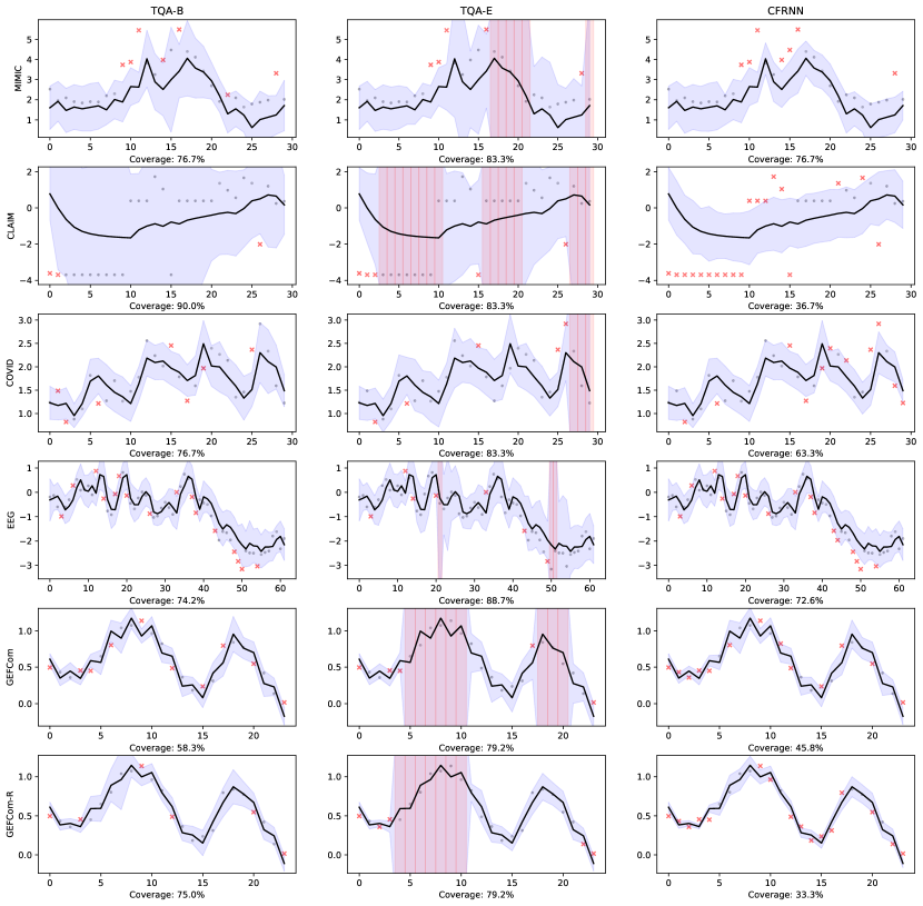
Evaluation Metrics and Experiment Setup We use RNN as the base point estimator due to its flexibility and for comparison with [45]. We use $\alpha=0.1$, and a LSTM ([17]) similar to that in [45] (full implementation details in the Appendix). For TQA-E, we use $\gamma=0.005$ following [15]. For each dataset, we repeat the prediction task 50 times, and report the mean and standard deviation of the average coverage rate, tail coverage rate, and inverse coverage efficiency for the last 20 time-steps. Here, tail coverage rate means the average coverage rate of the least-covered 10% of the time series. A high tail coverage rate thus implies better longitudinal coverage. Inverse coverage efficiency is measured by the average PI width divided by the marginal coverage rate (the smaller the better). Since TQA-E could create infinite PIs, we replace $\infty$ with 2x the widest finite PI. We also include in the Appendix results on full time series, and with Linear Regression instead of LSTM to show the model-agnostic nature of TQA.

Note that although we use equal-length time series in these experiments, for data with variable lengths (such as CLAIM or MIMIC), one could filter the calibration set before querying the quantile. As long as we assume exchangeability conditioning on length, all theoretical analysis still holds.

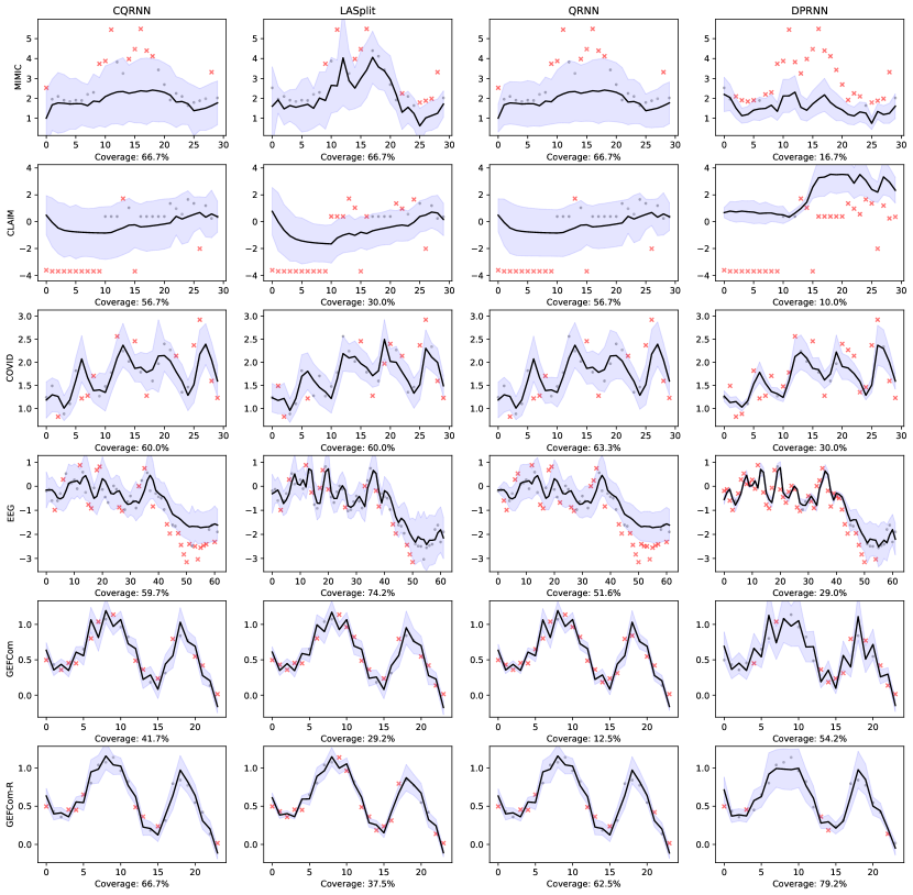
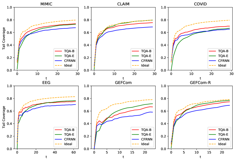
Results The results are presented in Tables 5, 5, and 5. In Table 5, we verify that conformal prediction methods - CFRNN (Split), CQRNN, LASplit and TQA- are empirically cross-sectionally valid. The non-conformal methods (QRNN and DPRNN) have unreliable coverage. In Table 5, we show that TQA can greatly improve the (longitudinal) average coverage rate for the worst TS. (TQA-E is consistently better than TQA-B due to the presence of infinitely-wide PIs.) This is also visualized in Figure 4. Note that although CQRNN and LASplit do not perform quantile adjustment, they model uncertainty directly, which also helps improve the longitudinal coverage but is less robust. In Table 5, we verify that TQA did not achieve better coverage simply by using very wide PIs (which is however the case for DPRNN on GEFCom). This is somewhat surprising because from Figure 4, the marginal gain in coverage decreases fast as $a_{t}$ decreases. The PIs for TQA-B should be wider due to the slight over-coverage, and the convexity (with any quantile adjustment). This suggests that TQA-B performs the budgeting very efficiently to cancel out both effects. The efficiency of TQA-E seems low due to the infinitely-wide PIs (replaced by 2x maximum finite width in this computation), but we will see that it generates mostly finite PIs, and the median width is still competitive.

Finally, we would like to also emphasize that any nonconformity scores could theoretically be combined with TQA. In this paper, and in our experiments, we mostly tried to combine the simplest nonconformity scores used in CFRNN (Split) with TQA. The question of how to combine TQA with other nonconformity scores (such as those used in CQRNN or LASplit) is left for future research.

Table 2: Average coverage rate. Empirically valid methods are in bold (at p = 0.01). As expected, conformal baselines are valid, while others (QRNN and DPRNN) are not. Note that GEFCom does not satisfy the exchangeability assumption, causing invalid coverage for most conformal methods. However, TQA still outperforms all conformal baselines, with TQA-E still valid.

Coverage	TQA-B	TQA-E	CFRNN (Split)	CQRNN	LASplit	QRNN	DPRNN
MIMIC	91.31$\pm$1.32	91.19$\pm$0.48	90.06$\pm$1.73	90.15$\pm$1.24	90.33$\pm$1.54	86.90$\pm$1.22	46.30$\pm$3.84
CLAIM	91.10$\pm$0.49	91.56$\pm$0.35	90.21$\pm$0.56	90.15$\pm$0.68	90.20$\pm$0.64	85.90$\pm$0.78	24.79$\pm$0.85
COVID	90.79$\pm$1.45	91.73$\pm$0.85	90.25$\pm$1.69	90.08$\pm$1.62	90.18$\pm$1.46	89.19$\pm$1.54	67.51$\pm$3.76
EEG	90.73$\pm$1.21	90.63$\pm$0.75	89.92$\pm$1.44	89.99$\pm$1.76	89.80$\pm$1.15	87.96$\pm$0.82	39.24$\pm$1.30
GEFCom	89.58$\pm$0.25	90.94$\pm$0.14	88.61$\pm$0.16	89.16$\pm$0.17	88.96$\pm$0.18	80.40$\pm$1.36	89.50$\pm$0.73
GEFCom-R	90.56$\pm$0.64	90.72$\pm$0.45	89.92$\pm$0.78	90.07$\pm$0.63	89.95$\pm$0.72	85.49$\pm$1.08	91.03$\pm$0.76

Table 3: The tail coverage rate (mean longitudinal coverage for the least-covered 10% TS), the higher the better. The best method is in bold, and the best method without using any infinitely-wide PI is underscored. Both versions of TQA consistently outperform all baselines.

Tail Coverage Rate $\uparrow$	TQA-B	TQA-E	CFRNN (Split)	CQRNN	LASplit	QRNN	DPRNN
MIMIC	71.59$\pm$4.03	80.68$\pm$1.74	62.22$\pm$7.09	68.60$\pm$3.84	65.05$\pm$6.12	61.80$\pm$3.91	17.24$\pm$5.38
CLAIM	74.16$\pm$1.22	81.53$\pm$0.77	65.95$\pm$1.88	66.45$\pm$3.19	68.08$\pm$2.44	53.89$\pm$3.59	1.65$\pm$0.54
COVID	70.01$\pm$4.45	82.39$\pm$1.28	64.41$\pm$6.11	66.41$\pm$5.99	67.38$\pm$4.63	65.16$\pm$6.15	36.65$\pm$5.63
EEG	70.99$\pm$2.18	79.03$\pm$1.22	64.14$\pm$3.42	61.95$\pm$4.71	67.13$\pm$2.32	57.82$\pm$2.78	12.99$\pm$1.32
GEFCom	68.96$\pm$1.70	81.77$\pm$0.36	58.49$\pm$1.38	61.63$\pm$1.56	60.46$\pm$1.66	47.56$\pm$2.27	67.45$\pm$1.69
GEFCom-R	75.28$\pm$1.28	81.80$\pm$0.69	68.76$\pm$2.18	71.95$\pm$1.66	70.79$\pm$2.12	64.99$\pm$1.92	71.86$\pm$1.75

Table 4: Inverse Efficiency, measured by the mean PI width divided by the coverage rate. Since TQA-E can create infinite PI, the width is computed by replacing $\infty$ with 2x the maximum finite PI width. The most efficient (and valid) method is in bold (p-value=0.01). As we can see, TQA-B is highly competitive in efficiency.

Inverse Efficiency $\downarrow$	TQA-B	TQA-E	CFRNN (Split)	CQRNN	LASplit	QRNN	DPRNN
MIMIC	1.990$\pm$0.165	2.382$\pm$0.265	1.964$\pm$0.170	1.738$\pm$0.145	2.072$\pm$0.223	1.623$\pm$0.146	1.258$\pm$0.132
CLAIM	3.020$\pm$0.045	3.279$\pm$0.074	3.003$\pm$0.052	2.902$\pm$0.044	3.009$\pm$0.064	2.691$\pm$0.035	2.401$\pm$0.205
COVID	0.831$\pm$0.032	1.167$\pm$0.337	0.826$\pm$0.034	0.908$\pm$0.091	0.826$\pm$0.037	0.888$\pm$0.096	0.744$\pm$0.050
EEG	1.449$\pm$0.025	1.749$\pm$0.125	1.445$\pm$0.031	1.586$\pm$0.052	1.448$\pm$0.025	1.497$\pm$0.042	1.061$\pm$0.027
GEFCom	0.238$\pm$0.005	0.280$\pm$0.013	0.235$\pm$0.005	0.242$\pm$0.005	0.238$\pm$0.005	0.211$\pm$0.005	0.636$\pm$0.009
GEFCom-R	0.200$\pm$0.004	0.222$\pm$0.010	0.198$\pm$0.004	0.207$\pm$0.004	0.201$\pm$0.004	0.193$\pm$0.004	0.590$\pm$0.009

6 Conclusions

In this paper, we proposed Temporal Quantile Adjustment, or TQA, to quantify uncertainty (create prediction intervals) in time series forecasting with a cross-section. TQA belongs to the framework of conformal prediction, and the main idea is to adjust the quantile to query using temporal information collected so far. This allows TQA to work with any model and any nonconformity score design. TQA theoretically is “no-worse” in cross-sectional coverage than vanilla split conformal as long as the expected value of adjustment is zero, and empirically improves the coverage. We also proposed two variants, TQA-B and TQA-E, both of which significantly outperform baselines in improving temporal/longitudinal coverage across many real world datasets. We hope that this work will serve as a foundation for the future design of PIs with both high cross-sectional and temporal coverage.

Checklist

The checklist follows the references. Please read the checklist guidelines carefully for information on how to answer these questions. For each question, change the default [TODO] to [Yes] , [No] , or [N/A] . You are strongly encouraged to include a justification to your answer, either by referencing the appropriate section of your paper or providing a brief inline description. For example:

• Did you include the license to the code and datasets? [Yes] See Section…

• Did you include the license to the code and datasets? [No] The code and the data are proprietary.

• Did you include the license to the code and datasets? [N/A]

Please do not modify the questions and only use the provided macros for your answers. Note that the Checklist section does not count towards the page limit. In your paper, please delete this instructions block and only keep the Checklist section heading above along with the questions/answers below.

1. For all authors…

   1. Do the main claims made in the abstract and introduction accurately reflect the paper’s contributions and scope? [Yes]

   2. Did you describe the limitations of your work? [Yes] TQA could theoretically lead to worse (although empirically better) coverage, as discussed in Section 4.

   3. Did you discuss any potential negative societal impacts of your work? [N/A] We do not foresee any potential negative societal impact of this work.

   4. Have you read the ethics review guidelines and ensured that your paper conforms to them? [Yes]

2. If you are including theoretical results…

   1. Did you state the full set of assumptions of all theoretical results? [Yes] Apart from exchangeability of time series (which we assume throughout this paper), any assumption is stated right before the relevant theorem.

   2. Did you include complete proofs of all theoretical results? [Yes] In the Appendix.

3. If you ran experiments…

   1. Did you include the code, data, and instructions needed to reproduce the main experimental results (either in the supplemental material or as a URL)? [Yes] In the supplemental material and will be published if accepted.

   2. Did you specify all the training details (e.g., data splits, hyperparameters, how they were chosen)? [Yes] In the Appendix.

   3. Did you report error bars (e.g., with respect to the random seed after running experiments multiple times)? [Yes] We repeat all experiments 50 times.

   4. Did you include the total amount of compute and the type of resources used (e.g., type of GPUs, internal cluster, or cloud provider)? [Yes] In Appendix.

4. If you are using existing assets (e.g., code, data, models) or curating/releasing new assets…

   1. If your work uses existing assets, did you cite the creators? [Yes]

   2. Did you mention the license of the assets? [Yes] In Appendix.

   3. Did you include any new assets either in the supplemental material or as a URL? [N/A]

   4. Did you discuss whether and how consent was obtained from people whose data you’re using/curating? [Yes] Most datasets are publicly available, except for CLAIM which is proprietary and provided to us by a company.

   5. Did you discuss whether the data you are using/curating contains personally identifiable information or offensive content? [Yes] They have been de-identified if applicable.

5. If you used crowdsourcing or conducted research with human subjects…

   1. Did you include the full text of instructions given to participants and screenshots, if applicable? [N/A]

   2. Did you describe any potential participant risks, with links to Institutional Review Board (IRB) approvals, if applicable? [N/A]

   3. Did you include the estimated hourly wage paid to participants and the total amount spent on participant compensation? [N/A]

Appendix A Proofs

A.1 Proof for Theorem 4.1

Proof.

Denote $\hat{r}_{N+1,t}=1-\alpha+\hat{\delta}_{N+1,t}$. To simplify the notation, in the following, all $\mathbb{P}$ means $\mathbb{P}_{\mathbf{S}_{N+1}\sim\mathcal{P}_{S}}$. We have:

$$\mathbb{P}\{Y_{N+1,t}\in\hat{C}_{a_{N+1,t},N+1,t}\} \geq\mathbb{P}\{rank_{N+1,t}\leq\hat{r}_{N+1,t}\}$$ (11)

$$=\int_{0}^{1}\int_{0}^{q}f_{rank_{N+1,t},\hat{r}_{N+1,t}}(r,q)drdq$$ (12)

$$=\int_{0}^{1}\int_{0}^{q}f_{rank_{N+1,t}}(r)f_{\hat{r}_{N+1,t}}(q)drdq$$ (13)

$$=\int_{0}^{1}qf_{\hat{r}_{N+1,t}}(q)dq$$ (14)

$$=\mathbb{E}[\hat{r}_{N+1,t}]=1-\alpha+\mathbb{E}[\hat{\delta}_{N+1,t}]$$ (15)

∎

A.2 Proof for Theorem 4.2

Proof.

For any $t$, we know that $\hat{r}_{N+1,t}$ follows a uniform distribution among $\{\frac{j}{N}\}_{j=0}^{N}$ by exchangeability. For simplicity, we drop the subscripts $\cdot_{N+1,t}$. As a result, we have

$$\mathbb{E}[\hat{r}|\hat{r}\geq 1-\alpha] =\frac{\lceil(1-\alpha)N\rceil+N}{2N}$$ (16)

$$\mathbb{E}[\hat{r}|\hat{r}<1-\alpha] =\frac{\lceil(1-\alpha)N\rceil-1}{2N}$$ (17)

More over,

$$\mathbb{P}\{\hat{r}\geq 1-\alpha\} =1-\frac{\lceil(1-\alpha)N\rceil}{N+1}$$ (18)

$$\mathbb{P}\{\hat{r}<1-\alpha\} =\frac{\lceil(1-\alpha)N\rceil}{N+1}.$$ (19)

Denoting $\epsilon\vcentcolon=\alpha N-\lfloor\alpha N\rfloor=\lceil(1-\alpha)N\rceil-(1-\alpha)N$, this means

$$\mathbb{E}[g^{B}(\hat{r};\alpha)] =\Bigg{(}1-\frac{\lceil(1-\alpha)N\rceil}{N+1}\Bigg{)}\Bigg{(}\frac{\lceil(1-\alpha)N\rceil+N}{2N}-(1-\alpha)\Bigg{)}$$ (20)

$$\mspace{150.0mu}+C\frac{\lceil(1-\alpha)N\rceil}{N+1}\Bigg{(}\frac{\lceil(1-\alpha)N\rceil-1}{2N}-(1-\alpha)\Bigg{)}$$ (21)

$$=\Bigg{(}1-\frac{(1-\alpha)N+\epsilon}{N+1}\Bigg{)}\Bigg{(}\frac{(2-\alpha)N+\epsilon}{2N}-(1-\alpha)\Bigg{)}$$ (22)

$$\mspace{150.0mu}+C\frac{(1-\alpha)N+\epsilon}{N+1}\Bigg{(}\frac{(1-\alpha)N-1+\epsilon}{2N}-(1-\alpha)\Bigg{)}$$ (23)

$$=\Bigg{(}\frac{\alpha N+1-\epsilon}{N+1}\Bigg{)}\Bigg{(}\frac{\alpha N+\epsilon}{2N}\Bigg{)}$$ (24)

$$\mspace{150.0mu}+C\frac{(1-\alpha)N+\epsilon}{N+1}\Bigg{(}\frac{(\alpha-1)N-1+\epsilon}{2N}\Bigg{)}$$ (25)

$$=\frac{\alpha^{2}N^{2}+\alpha N+\epsilon-\epsilon^{2}}{2(N+1)N}-C\frac{(1-\alpha)^{2}N^{2}+(1-\alpha)N+\epsilon-\epsilon^{2}}{2(N+1)N}$$ (26)

As a result,

$$\mathbb{E}[g^{B}(\hat{r};\alpha)]=0\Leftrightarrow C=\frac{(\alpha N+\epsilon)(\alpha N+1-\epsilon)}{((1-\alpha)N+\epsilon)((1-\alpha)N+1-\epsilon)}$$ (28)

∎

A.3 Proof for Theorem 4.3

Proof.

The inequality trivially holds for $\alpha\geq 0.5$, so we only focus on the case when $\alpha<0.5$.

An upper-bound for the additional loss is simply $L\vcentcolon=-\min_{q}g^{B}(q;\alpha)$. To find an upper bound for $L$, notice that

$$L=-\min_{q}g^{B}(q;\alpha) =(1-\alpha)C$$ (29)

$$=\frac{(\alpha N+\epsilon)(\alpha N+1-\epsilon)}{((1-\alpha)N+\epsilon)((1-\alpha)N+1-\epsilon)}(1-\alpha)$$ (30)

$$=\frac{\alpha^{2}N^{2}+\alpha N+\epsilon-\epsilon^{2}}{(1-\alpha)^{2}N^{2}+(1-\alpha)N+\epsilon-\epsilon^{2}}(1-\alpha)$$ (31)

$$=\Big{(}1-\frac{N^{2}[(1-\alpha)^{2}-\alpha^{2}]+N(1-2\alpha)}{(1-\alpha)^{2}N^{2}+(1-\alpha)N+\epsilon-\epsilon^{2}}\Big{)}(1-\alpha)$$ (32)

If we consider the last expression as a function of $\epsilon$, it is maximized with $\epsilon=\frac{1}{2}$, which means

$$L\leq\Bigg{(}\frac{\alpha+\frac{1}{2N}}{1-\alpha+\frac{1}{2N}}\Bigg{)}^{2}(1-\alpha)$$ (33)

Denote $\alpha^{+}\vcentcolon=\alpha+\Bigg{(}\frac{\alpha+\frac{1}{2N}}{1-\alpha+\frac{1}{2N}}\Bigg{)}^{2}(1-\alpha)$. We have $\hat{C}^{split}_{\alpha^{+},N+1,t+1}\subseteq\hat{C}^{TQA-B}_{\alpha,N+1,t+1}$. This means

$$\mathbb{P}_{\mathbf{S}_{N+1}\sim\mathcal{P}_{S}}\{Y_{N+1,t+1}\in\hat{C}^{TQA-B}_{\alpha,N+1,t+1}\}$$ (34)

$$\geq\mathbb{P}_{\mathbf{S}_{N+1}\sim\mathcal{P}_{S}}\{Y_{N+1,t+1}\in\hat{C}^{split}_{\alpha^{+},N+1,t+1}\}$$ (35)

$$\geq 1-\alpha-\Bigg{(}\frac{\alpha+\frac{1}{2N}}{1-\alpha+\frac{1}{2N}}\Bigg{)}^{2}(1-\alpha)$$ (36)

∎

A.4 Proof for Theorem 4.4

Proof.

First, let us consider the alternative quantile adjustment $b^{TQA-E}_{N+1,t}$ with update rule:

$$b_{t+1}\leftarrow\begin{cases}b_{t}+\gamma(\alpha-err_{t})&(b_{t}\in[0,1])\\ b_{t}+\gamma(\alpha-b_{t})&(otherwise)\end{cases}.$$ (37)

We will first show $\forall t,\mathbb{E}[b_{t}]=\alpha$ by induction, as we hinted in the main paper. (For simplicity in notation, we drop the subscript $\cdot_{N+1}$.) To begin with, we have

$$\mathbb{E}_{\mathbf{S}}[b^{TQA-E}_{0}]=\mathbb{E}_{\mathbf{S}}[\alpha]=\alpha$$ (38)

Now,

$$\mathbb{E}_{\mathbf{S}}[b_{t+1}|b_{t}] =\begin{cases}b_{t}+\gamma(\alpha-\mathbb{E}_{\mathbf{S}}[err_{t}])&(b_{t}\in[0,1])\\ b_{t}+\gamma(\alpha-b_{t})&(otherwise)\end{cases}$$ (39)

If the nonconformity score’s rank has no temporal dependence, we have $err_{t}\sim Bernoulli(a_{t})$ (here again we assume we use random coin-flips to ensure an exact coverage probability of $1-\alpha$), which means $\mathbb{E}[err_{t}]=b_{t}$. This leads to

$$\mathbb{E}_{\mathbf{S}}[b_{t+1}|b_{t}]=b_{t}+\gamma(\alpha-b_{t})$$ (40)

$$\implies \mathbb{E}_{\mathbf{S}}[b_{t+1}]=\mathbb{E}_{\mathbf{S}}[\mathbb{E}_{\mathbf{S}}[b_{t+1}|b_{t}]]=(1-\gamma)\mathbb{E}_{\mathbf{S}}[b_{t}]+\gamma\alpha=\alpha$$ (41)

By induction, we have

$$\forall t,\mathbb{E}_{\mathbf{S}}[b_{t}]=\alpha$$ (42)

Next, we should compare $\mathbb{E}[a_{t}]$ and $\mathbb{E}[b_{t}]$. It should be clear that

$$\forall c,\mathbb{E}_{\mathbf{S}}[a_{t+1}|a_{t}=c]\leq\mathbb{E}_{\mathbf{S}}[b_{t+1}|b_{t}=c].$$ (43)

To begin with, we have $\mathbb{E}[a_{0}]\leq\alpha$. Following a similar logic, we have

$$\mathbb{E}_{\mathbf{S}}[a_{t+1}]=\mathbb{E}_{\mathbf{S}}[\mathbb{E}_{\mathbf{S}}[a_{t+1}|a_{t}]]\leq(1-\gamma)\mathbb{E}_{\mathbf{S}}[a_{t}]+\gamma\alpha\leq\alpha$$ (44)

By induction, we get

$$\forall t,\mathbb{E}_{\mathbf{S}_{N+1}\sim\mathcal{P}_{S}}[a^{TQA-E}_{N+1,t}]\leq\alpha.$$ (45)

∎

Remarks The alternative update rule in Eq. 37 is not just used to prove Theorem 4.4. In fact, one might want to use this rule in practice if the TS is not very long and the asymptotic guarantee (Theorem 4.5) is not relevant. This is because Eq. 37 does not become more conservative on average as $t$ increases.

A.5 Proof for Theorem 4.5

Proof.

We will use an similar argument similar to one in [15]. First, we have $a_{t}\in[-\gamma,1+\gamma]$ if $a_{0}=\alpha$. To see this, note that $a_{t+1}>a_{t}\implies a_{t}\leq 1\implies a_{t+1}\leq 1+\gamma$, which means $\forall t,a_{t}\leq 1+\gamma$. Similarly, $a_{t+1}<a_{t}\implies a_{t}\geq 0\implies a_{t+1}\geq-\gamma$, which means $\forall t,a_{t}\geq-\gamma$.

Note that with Eq. 9, we have $a_{t+1}\leq a_{t}+\gamma(\alpha-a_{t})$. Now, if we expand $a_{T}$, we get

$$-\gamma\leq a_{T}\leq\alpha+\sum_{t=0}^{T-1}\gamma(\alpha-err_{t})$$ (46)

$$\implies \frac{\sum_{t=0}^{T-1}err_{t}}{T}\leq\alpha+\frac{\alpha+\gamma}{\gamma T}$$ (47)

By taking the limit of both sides, we are done.

∎

Appendix B Additional Experiment Details

B.1 Datasets

MIMIC [21, 16, 20]: MIMIC-III is a large public (but requires application of access) database consisting of records for patients admitted to critical care units. The task is to predict white blood cell counts (WBCC) levels, using 25 features (following [1]) including measurements like systolic/diastolic blood pressure or the dosage of antibiotics. To prepare the data, we follow [45] and restrict our study to patients on antibiotics (Levofloxacin). We drop sequences with less than 30 visits, ending up with 392 sequences in total. The exact SQL queries and data processing scripts are provided in the supplemental material and will be published. Note that the EHR has been de-identified - in particular, all visits for a patient are shifted in dates, so we only know the relative dates of visits belonging to the same patient, but do not know the actual dates, making it impossible to perform any temporal splitting.

CLAIM: CLAIM is a proprietary dataset from a large healthcare data provider in North America. It contains longitudinal view of information like inpatient and outpatient services, prescription, costs or enrollment. The task is to predict the (allowed) claim amount for the next visit. The features include diagnoses codes (ICD-10) and procedure codes (CPT/HCPCS), the gender and age of patient, and the previous claim amount.

COVID [10]: COVID is available at https://coronavirus.data.gov.uk/. We follow the setup of [45] and treat different regions within UK as the cross-section, and we used the most recent full-month data available at the time of this work (March 2022). The feature only consists of previous day’s case number. We include COVID for completeness as it was used in [45], and as an idealized experiment, despite its unrealistic settings.

EEG [48]: EEG is available at https://archive.ics.uci.edu/ml/datasets/EEG+Database. The “Large” version of the dataset contains the electroencephalography (EEG) signals sampled at 256 Hz for 1 second for 10 alcoholic and 10 control subjects. Like [45], we used only the control group, and downsampled the signals to facilitate training, but to length 64 instead of 50 to avoid unnecessary interpolation. We do not mix data from different EEG channels, and use only channel 0 data because different EEG channels should follow different developments. The feature only consists of the EEG signal at the previous step.

GEFCom [18]: GEFCom (2014) is the Probabilistic Electric Load Forecasting task in Global Energy Forecasting Competition 2014. It has hourly temperature and electricity load data for one utility. The load data covers 9 years. For this task, we split the data into 24-hour-sequences, and consider these sequences as forming a cross-section. The features consist of temperature data from 25 stations, and the previous load.

Data Licenses and Consent:

• MIMIC: The PhysioNet Credentialed Health Data License. The data is public, but requires access application.

• COVID: Open Government Licence v3.0. Publicly available on https://coronavirus.data.gov.uk/.

• CLAIM: This is proprietary data.

• EEG: There are no usage restrictions on this data per https://archive.ics.uci.edu/ml/datasets/eeg+database.

• GEFCom: We could not find the license, but it is publicly available (provided by the author) on http://blog.drhongtao.com/2017/03/gefcom2014-load-forecasting-data.html.

B.2 Implementation and Experiment Details

We use mostly the same architecture and training protocols as [45]. The RNN (mean estimator) is a one-layer LSTM [17], with an embedding size of 32. The optimizer is ADAM [22], and the learning rate is 1e-3. The training epochs for MIMIC/CLAIM/COVID/EEG/GEFCom are 200/500/1000/100/1000. We use the same settings for the residual predictor (for LASplit) and QRNN, except that

• The target for the residual predictor is replaced by $|y-\hat{y}|$.

• The loss for QRNN is replaced with the quantile loss, and the output is two scalars instead of one.

We normalize each feature and $Y$ by the mean and standard deviation in order for the underlying LSTM to train. In each repetition of a experiments, we pool all data together and re-split them into training/calibration/test set using a new seed, and the LSTMs are also trained using different seeds each time. The only exception is GEFCom (the non-R version), which has only one data splitting due to the temporal order. The LSTMs for GEFCom are still trained using different seeds. All code is provided in the supplemental material and will be published after the review period.Experiments in this paper are fast to run on a personal laptop - the largest single experiment is for CLAIM (without repetition), which takes about half an hour, and all experiments finish within 2 hours (for one seed).

Appendix C Variants of TQA-B

C.1 Rank-based Quantile Prediction

Instead of the quantile prediction we used in the paper, we also tried the following prediction. $\hat{r}^{ewa}_{i,t+1}=Q^{-1}(\overline{r}_{i,t};\{\overline{r}_{j,t}\}_{j=1}^{N+1})$ where $\overline{r}_{i,t}\vcentcolon=\frac{\sum_{t^{\prime}=1}^{t}\beta^{t+1-t^{\prime}}r_{i,t^{\prime}}}{\sum_{t^{\prime}=1}^{t}\beta^{t+1-t^{\prime}}}$. This is an exponentially weighted (decaying) average of the past ranks. We use $\beta=0.8$, and refer to such quantile prediction as Rank-based (as opposed to Scaled-based in Section 4.2).

C.2 The Aggressive Quantile Budgeting

Figure 5: Here we present visualizations of different quantile budgeting methods. “Budgeting” refers to the fact that all red lines are on average $1-\alpha$. The first picture (No Adjustment) is the same as the basic split conformal method. The second picture refers to the quantile budgeting method presented in Section 4.2. It is conservative because even for a very small $\hat{r}_{t}$ like 0, the adjusted $a_{t}$ is still close to $\alpha$. The third picture is the more aggressive budgeting method, and it could set $a_{t}$ to as big as $2\alpha$. In a sense, it trusts the prediction $\hat{r}_{t}$ and adapts to it more. As a result, if $\hat{r}_{t}$ predicts the actual rank of nonconformity scores well, it can achieve a much higher coverage. The extreme case is if $\hat{r}_{t}$ perfectly predicts the realized ranks: “No Adjustment” will still have $1-\alpha$ coverage whereas the other two will achieve perfect coverage.

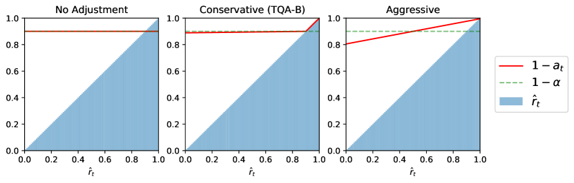
In this section, we present an alternative quantile budgeting function to $g^{B}$. The specific adjustment is given by

$$g^{BC}(q;\alpha) \vcentcolon=\frac{q-0.5}{2\alpha}.$$ (48)

Like in Section 4.2, one could use a $\lambda$ to ensure the final $a_{t}$ is not too close to zero (to avoid infinitely-wide PIs). We refer to this “aggressive” version as TQA-BC. Figure 5 visualizes the difference between “conservative” (TQA-B) and “aggressive” budgeting. It should be clear that TQA-BC also satisfies Theorem 4.2, Theorem 4.3, however, becomes looser:

Theorem C.1.

$$\mathbb{P}_{\mathbf{S}_{N+1}\sim\mathcal{P}_{S}}\{Y_{N+1,t+1}\in\hat{C}^{TQA-BC}_{\alpha,N+1,t+1}\}\geq 1-2\alpha.$$ (49)

The proof is essentially the same as that for Theorem 4.3.

C.3 Comparison

The full results of different variants of TQA-B are in Table C.3. All variants are generally valid (except for a tiny drop in coverage for Rank+Conservative on GEFCom-R). In general, among the two quantile prediction methods, Scale tends to produce better tail coverage rate, at the cost of worse efficiency. Among the quantile budgeting methods, the Aggressive version also tends to increase tail coverage rate and decrease efficiency. In practice, one might design the two components depending on the whether efficiency or tail coverage rate is more important.

Table 5: Mean coverage, tail coverage, and inverse efficiency for different variants of TQA-B. Valid mean coverage and the best of tail coverage and inverse efficiency are in bold. Note that we re-scaled all methods’ mean PI width to the same as CFRNN for the TCR here, for a fair comparison. (We couldn’t do this in a meaningful way for TQA-E in the main text.)

	TQA-B				CFRNN (Split)
Quantile Prediction Method	Scale		Rank
Budgeting Method	Conservative	Aggressive	Conservative	Aggressive
Coverage
MIMIC	91.31$\pm$1.32	93.62$\pm$1.04	89.79$\pm$1.68	91.79$\pm$1.41	90.06$\pm$1.73
CLAIM	91.19$\pm$0.48	92.87$\pm$0.37	89.88$\pm$0.55	91.54$\pm$0.46	90.21$\pm$0.56
COVID	90.79$\pm$1.45	92.46$\pm$1.15	89.94$\pm$1.71	91.16$\pm$1.44	90.25$\pm$1.69
EEG	90.73$\pm$1.21	92.53$\pm$1.00	89.57$\pm$1.46	90.95$\pm$1.28	89.92$\pm$1.44
GEFCom	89.58$\pm$0.25	91.19$\pm$0.39	87.96$\pm$0.20	89.62$\pm$0.22	88.61$\pm$0.16
GEFCom-R	90.56$\pm$0.64	91.52$\pm$0.57	89.55$\pm$0.80	90.57$\pm$0.67	89.92$\pm$0.78
Tail Coverage Rate (rescaled) $\uparrow$
MIMIC	70.18$\pm$4.17	76.84$\pm$4.20	63.06$\pm$6.46	70.98$\pm$4.69	62.22$\pm$7.09
CLAIM	73.36$\pm$1.27	78.15$\pm$1.20	66.73$\pm$1.76	73.08$\pm$1.29	65.95$\pm$1.88
COVID	69.48$\pm$4.48	75.49$\pm$4.89	64.85$\pm$5.80	69.44$\pm$5.51	64.41$\pm$6.11
EEG	70.29$\pm$2.15	75.81$\pm$2.69	64.50$\pm$3.32	69.51$\pm$3.01	64.14$\pm$3.42
GEFCom	67.71$\pm$1.68	74.19$\pm$2.55	58.51$\pm$1.27	67.52$\pm$1.42	58.49$\pm$1.38
GEFCom-R	74.48$\pm$1.36	77.47$\pm$1.36	69.18$\pm$2.14	73.59$\pm$1.58	68.76$\pm$2.18
Inverse Efficiency $\downarrow$
MIMIC	1.990$\pm$0.165	2.128$\pm$0.182	1.936$\pm$0.166	1.979$\pm$0.166	1.964$\pm$0.170
CLAIM	3.020$\pm$0.045	3.224$\pm$0.072	2.956$\pm$0.051	3.025$\pm$0.046	3.003$\pm$0.052
COVID	0.831$\pm$0.032	0.858$\pm$0.036	0.819$\pm$0.033	0.828$\pm$0.033	0.826$\pm$0.034
EEG	1.449$\pm$0.025	1.498$\pm$0.023	1.429$\pm$0.029	1.444$\pm$0.025	1.445$\pm$0.031
GEFCom	0.238$\pm$0.005	0.247$\pm$0.007	0.233$\pm$0.005	0.236$\pm$0.005	0.235$\pm$0.005
GEFCom-R	0.200$\pm$0.004	0.210$\pm$0.006	0.196$\pm$0.004	0.199$\pm$0.004	0.198$\pm$0.004

Appendix D Additional Results

Full Time Series: We repeat the experiments in Section 5 but measure the evaluation metrics on the entire time series as opposed to the last 20 steps. The results are in Table D and the conclusion stays the same.

Table 6: Mean coverage, tail coverage, and inverse efficiency using the entire time series (as opposed to the last 20 steps). Valid mean coverage and the best of tail coverage and inverse efficiency are in bold. The conclusion is the same as in the main text - TQA greatly improves the longitudinal coverage for the least-covered TSs, and in particular TQA-B maintains very competitive efficiency.

Coverage	TQA-B	TQA-E	CFRNN (Split)	CQRNN	LASplit	QRNN	DPRNN
MIMIC	91.16$\pm$1.15	91.76$\pm$0.63	90.03$\pm$1.49	90.06$\pm$1.17	90.19$\pm$1.32	84.81$\pm$1.13	44.78$\pm$3.61
CLAIM	91.00$\pm$0.37	91.38$\pm$0.23	90.13$\pm$0.48	90.07$\pm$0.54	90.11$\pm$0.44	86.38$\pm$0.62	25.31$\pm$0.72
COVID	90.70$\pm$1.39	91.73$\pm$0.74	90.18$\pm$1.61	90.08$\pm$1.44	90.15$\pm$1.39	89.11$\pm$1.45	65.40$\pm$2.74
EEG	90.56$\pm$0.85	91.04$\pm$0.30	89.82$\pm$1.07	89.99$\pm$1.14	89.82$\pm$0.96	86.82$\pm$0.62	35.35$\pm$1.18
GEFCom	89.34$\pm$0.23	90.62$\pm$0.12	88.50$\pm$0.15	89.05$\pm$0.16	88.83$\pm$0.16	80.58$\pm$1.29	90.46$\pm$0.73
GEFCom-R	90.56$\pm$0.60	90.69$\pm$0.39	89.95$\pm$0.75	90.13$\pm$0.61	89.97$\pm$0.66	85.86$\pm$1.08	91.97$\pm$0.71
Tail Coverage Rate $\uparrow$
MIMIC	75.22$\pm$3.08	84.64$\pm$0.95	67.54$\pm$4.99	71.42$\pm$3.58	69.76$\pm$4.47	62.53$\pm$3.73	21.16$\pm$4.37
CLAIM	76.26$\pm$0.91	84.60$\pm$0.39	68.76$\pm$1.71	69.75$\pm$2.50	71.21$\pm$1.87	59.78$\pm$2.85	4.55$\pm$0.56
COVID	70.47$\pm$4.65	84.21$\pm$0.89	65.22$\pm$5.83	68.70$\pm$5.71	69.07$\pm$4.59	67.19$\pm$5.72	40.74$\pm$4.24
EEG	75.80$\pm$1.25	87.22$\pm$0.13	70.43$\pm$2.17	69.94$\pm$2.80	71.62$\pm$1.77	65.22$\pm$1.93	18.86$\pm$0.94
GEFCom	67.84$\pm$1.66	82.71$\pm$0.15	58.26$\pm$1.20	61.72$\pm$1.48	60.36$\pm$1.63	48.51$\pm$2.06	71.45$\pm$1.54
GEFCom-R	75.41$\pm$1.26	83.00$\pm$0.31	69.14$\pm$2.10	72.96$\pm$1.57	71.51$\pm$1.88	66.64$\pm$1.98	75.65$\pm$1.71
Inverse Efficiency $\downarrow$
MIMIC	2.053$\pm$0.157	2.478$\pm$0.333	2.018$\pm$0.152	1.831$\pm$0.153	2.115$\pm$0.185	1.676$\pm$0.148	1.277$\pm$0.120
CLAIM	3.039$\pm$0.038	3.245$\pm$0.061	3.019$\pm$0.043	2.934$\pm$0.039	3.023$\pm$0.051	2.740$\pm$0.031	2.242$\pm$0.146
COVID	0.823$\pm$0.031	1.112$\pm$0.246	0.819$\pm$0.033	0.876$\pm$0.073	0.817$\pm$0.038	0.857$\pm$0.077	0.728$\pm$0.047
EEG	1.374$\pm$0.016	1.662$\pm$0.093	1.368$\pm$0.022	1.494$\pm$0.039	1.368$\pm$0.018	1.414$\pm$0.033	0.985$\pm$0.017
GEFCom	0.222$\pm$0.005	0.257$\pm$0.011	0.219$\pm$0.004	0.225$\pm$0.004	0.221$\pm$0.004	0.195$\pm$0.004	0.618$\pm$0.009
GEFCom-R	0.185$\pm$0.003	0.203$\pm$0.009	0.183$\pm$0.003	0.191$\pm$0.004	0.186$\pm$0.004	0.178$\pm$0.004	0.589$\pm$0.009

Percentage of Infinitely-wide PIs: Since TQA-E could generate infinitely-wide PIs, we check how many such intervals are actually created. The results are in Table D, and it shows that most $\hat{C}^{TQA-E}$ are finite.

Table 7: The percentage of infinitely-wide PIs created by TQA-E for different datasets. Only a very small percentage of the PIs are infinitely-wide.

% Infinitely-wide PI	MIMIC	CLAIM	COVID	EEG	GEFCom	GEFCom-R
Last 20 steps	3.10$\pm$1.23	2.18$\pm$0.36	3.40$\pm$1.47	3.78$\pm$0.97	3.84$\pm$0.17	2.31$\pm$0.52
Full TS	2.51$\pm$0.99	1.72$\pm$0.28	2.74$\pm$1.24	3.46$\pm$0.78	3.22$\pm$0.15	1.94$\pm$0.44

Median and Mean Width of the PIs: We examine the raw width of the PIs. Note that because TQA-B tends to improve the coverage slightly, the width is slightly higher. In addition, the mean width should be even higher due to the attempt to cover extreme residuals (as discussed/showed in Figure 4). However, from Table D, we note that the difference in the raw PI widths are also small.

Table 8: Median and mean width of the PIs. The widths of infinitely-wide $\hat{C}^{TQA-E}$ are replaced with 2x the width of the widest finite PI.

Median Width $\downarrow$	TQA-B	TQA-E	CFRNN (Split)	CQRNN	LASplit	QRNN	DPRNN
MIMIC	1.741$\pm$0.165	1.639$\pm$0.146	1.753$\pm$0.169	1.443$\pm$0.120	1.640$\pm$0.172	1.279$\pm$0.116	0.493$\pm$0.023
CLAIM	2.667$\pm$0.053	2.561$\pm$0.051	2.710$\pm$0.060	2.628$\pm$0.048	2.456$\pm$0.057	2.325$\pm$0.032	0.434$\pm$0.023
COVID	0.735$\pm$0.036	0.705$\pm$0.035	0.739$\pm$0.038	0.776$\pm$0.072	0.706$\pm$0.034	0.757$\pm$0.084	0.390$\pm$0.052
EEG	1.285$\pm$0.044	1.207$\pm$0.035	1.291$\pm$0.052	1.343$\pm$0.069	1.228$\pm$0.039	1.218$\pm$0.040	0.312$\pm$0.013
GEFCom	0.201$\pm$0.004	0.196$\pm$0.004	0.198$\pm$0.004	0.204$\pm$0.004	0.191$\pm$0.004	0.155$\pm$0.005	0.428$\pm$0.006
GEFCom-R	0.171$\pm$0.008	0.174$\pm$0.005	0.170$\pm$0.008	0.171$\pm$0.004	0.164$\pm$0.005	0.149$\pm$0.005	0.458$\pm$0.009
Mean Width $\downarrow$
MIMIC	1.818$\pm$0.157	2.189$\pm$0.245	1.769$\pm$0.164	1.566$\pm$0.132	1.872$\pm$0.212	1.411$\pm$0.130	0.578$\pm$0.031
CLAIM	2.754$\pm$0.048	3.002$\pm$0.070	2.709$\pm$0.056	2.616$\pm$0.049	2.714$\pm$0.067	2.312$\pm$0.033	0.594$\pm$0.042
COVID	0.755$\pm$0.033	1.070$\pm$0.308	0.746$\pm$0.038	0.818$\pm$0.084	0.745$\pm$0.037	0.792$\pm$0.088	0.503$\pm$0.050
EEG	1.315$\pm$0.039	1.585$\pm$0.111	1.299$\pm$0.048	1.428$\pm$0.069	1.300$\pm$0.037	1.317$\pm$0.043	0.416$\pm$0.017
GEFCom	0.213$\pm$0.005	0.255$\pm$0.012	0.208$\pm$0.004	0.216$\pm$0.004	0.212$\pm$0.005	0.170$\pm$0.005	0.569$\pm$0.007
GEFCom-R	0.181$\pm$0.004	0.201$\pm$0.010	0.178$\pm$0.005	0.187$\pm$0.004	0.181$\pm$0.005	0.165$\pm$0.005	0.537$\pm$0.011

CFRNN with Bonferroni Correction (CFRNN-Bon): As explained in Section 3.2, to perform the correct split conformal prediction, we need to use $\infty$ in place of $v_{N+1}$ (in order to avoid plugging in different $y$ values, usually defined on a fine-granular grid, which is very expensive). This means that, if we perform Bonferroni Correction as proposed in [45] by querying the $1-\frac{\alpha}{T}$ instead of $1-\alpha$, the PI will always by infinitely wide if $\frac{\alpha}{T}<=\frac{1}{N+1}$. In our experiments, this is the case for MIMIC, COVID, EEG and GEFCom/GEFCom-R. The original paper [45] implemented the split-conformal incorrectly by ignoring $v_{N+1}$, which is why this issue did not appear. In addition, even if we ignore the issue of (constant) infinitely-wide PIs, in our settings the length of the time-series (e.g. number of visits by a patient) might not be known in advance. As a result, it is not clear how to perform the Bonferroni Correction.

Tail coverage rate over time Figure 6 shows the tail coverage rate at different values of $t$. Ideal means the coverage is independent for different $t$ within each time series. In general TQA improves the tail coverage noticeably, but there is still gap between Ideal and TQA. TQA-E sometimes approaches this optimal case (at the expense of creating infinitely-wide PIs).

Figure 6: Tail Coverage Rate as a function of time. We plot the mean of 50 experiments. There is, however, still gap between TQA and Ideal.

Mean (cross-sectional) coverage over time Figure 7 shows the mean coverage rate for different $t$. As expected, conformal methods show cross-sectional validity, whereas the coverage rate for non-conformal methods vary.

Figure 7: Mean coverage rate at different $t$. Conformal methods are valid at all $t$. Coverage rate for non-conformal methods vary greatly through time.

Linear Regression: We repeat the experiments in Section 5 but replace the underlying LSTM with Linear Regression (by training one model for each $t$, taking input from up to $t-1$). The CLAIM data is skipped in this case due to difficulty in training. The results are in Table D and the conclusion stays the same.

Table 9: Mean coverage, tail coverage, and inverse efficiency with linear regression being the base point estimator. Valid mean coverage and the best of tail coverage and inverse efficiency are in bold. The conclusion is the same as the case of LSTM.

Coverage	TQA-B	TQA-E	CFRNN (Split)	CQR	LASplit
MIMIC	90.65$\pm$1.36	91.63$\pm$0.79	89.75$\pm$1.61	89.96$\pm$1.62	89.81$\pm$1.48
COVID	90.93$\pm$1.45	91.95$\pm$0.86	90.28$\pm$1.71	90.17$\pm$1.57	90.25$\pm$1.55
EEG	90.76$\pm$1.34	90.78$\pm$0.84	89.92$\pm$1.56	90.26$\pm$1.93	90.14$\pm$1.32
GEFCom	89.66$\pm$0.17	90.46$\pm$0.12	89.32$\pm$0.14	88.98$\pm$0.28	89.21$\pm$0.16
GEFCom-R	90.57$\pm$0.63	90.78$\pm$0.42	90.08$\pm$0.72	90.13$\pm$0.66	90.12$\pm$0.59
Tail Coverage Rate $\uparrow$
MIMIC	68.80$\pm$3.88	80.73$\pm$1.52	60.59$\pm$5.64	59.40$\pm$5.23	64.36$\pm$4.88
COVID	70.38$\pm$4.04	82.20$\pm$1.51	64.35$\pm$6.00	68.30$\pm$4.75	69.41$\pm$4.94
EEG	68.11$\pm$2.73	77.66$\pm$1.27	61.09$\pm$3.96	54.45$\pm$6.58	66.81$\pm$2.70
GEFCom	73.72$\pm$0.92	81.58$\pm$0.33	69.31$\pm$0.95	70.01$\pm$1.12	71.40$\pm$0.92
GEFCom-R	75.34$\pm$0.88	81.61$\pm$0.81	70.69$\pm$1.42	72.69$\pm$1.39	73.01$\pm$1.48
Inverse Efficiency $\downarrow$
MIMIC	3.235$\pm$0.263	4.092$\pm$0.768	3.205$\pm$0.266	2.899$\pm$0.252	3.326$\pm$0.286
COVID	0.898$\pm$0.028	1.129$\pm$0.171	0.893$\pm$0.030	0.921$\pm$0.042	0.894$\pm$0.028
EEG	1.840$\pm$0.048	2.232$\pm$0.152	1.832$\pm$0.057	1.976$\pm$0.080	1.995$\pm$0.059
GEFCom	0.309$\pm$0.005	0.350$\pm$0.007	0.307$\pm$0.005	0.373$\pm$0.011	0.334$\pm$0.006
GEFCom-R	0.297$\pm$0.006	0.318$\pm$0.009	0.296$\pm$0.007	0.355$\pm$0.008	0.315$\pm$0.006

Examples of Actual PIs Figure 8 how TQA-B and TQA-E improve the coverage for the least-covered TSs over CFRNN (Split) (as they use the same nonconformity score). The rest of the baselines are in Figure 9. We use random seed 1 and pick the 1-th-least-covered TS (according to the mean coverage across all baselines) from each dataset. In general, TQA would increase the width (by lowering $a_{t}$) if the first few observations of a TS shows some extremity, which is probably most noticeable in CLAIM. CQRNN and LASplit also adapt to the widths by using different nonconformity scores. Again, we note that the quality of TQA-B might be further improved with better prediction $\hat{r}$.

Figure 8: Dark lines are $\hat{y}$, blue bands are the PIs, and × denotes $y$ outside the PI. red bands means infinitely-wide PIs for TQA-E. The adaptive-ness of TQA-B and TQA-E may be most obvious in CLAIM and GEFCom-R. We also note that TQA-E seems to produce quite a few infinitely-wide PIs on these least-covered TSs (somewhat as expected).

Figure 9: Like Figure 8, but for different baselines.

References

- [1] Ahmed Alaa and Mihaela Van Der Schaar. Frequentist uncertainty in recurrent neural networks via blockwise influence functions. In Hal Daumé III and Aarti Singh, editors, Proceedings of the 37th International Conference on Machine Learning, volume 119 of Proceedings of Machine Learning Research, pages 175–190. PMLR, 13–18 Jul 2020.
- [2] Anastasios Nikolas Angelopoulos, Stephen Bates, Michael Jordan, and Jitendra Malik. Uncertainty sets for image classifiers using conformal prediction. In International Conference on Learning Representations, 2021.
- [3] Anastasios Nikolas Angelopoulos, Amit Kohli, Stephen Bates, Michael I. Jordan, Jitendra Malik, Thayer Alshaabi, Srigokul Upadhyayula, and Yaniv Romano. Image-to-image regression with distribution-free uncertainty quantification and applications in imaging. ArXiv, abs/2202.05265, 2022.
- [4] Rina Foygel Barber, Emmanuel J. Candes, Aaditya Ramdas, and Ryan J. Tibshirani. Conformal prediction beyond exchangeability, 2022.
- [5] Rina Foygel Barber, Emmanuel J. Candès, Aaditya Ramdas, and Ryan J. Tibshirani. The limits of distribution-free conditional predictive inference. arXiv, abs/1903.04684, 2020.
- [6] Stephen Bates, A. Angelopoulos, Lihua Lei, Jitendra Malik, and Michael I. Jordan. Distribution-free, risk-controlling prediction sets. J. ACM, 68:43:1–43:34, 2021.
- [7] Jose Caceres, Danilo Gonzalez, Taotao Zhou, and Enrique Lopez Droguett. A probabilistic bayesian recurrent neural network for remaining useful life prognostics considering epistemic and aleatory uncertainties. Structural Control and Health Monitoring, 28(10):e2811, 2021.
- [8] Tianqi Chen, Emily Fox, and Carlos Guestrin. Stochastic gradient hamiltonian monte carlo. In Eric P. Xing and Tony Jebara, editors, Proceedings of the 31st International Conference on Machine Learning, volume 32:2 of Proceedings of Machine Learning Research, pages 1683–1691, Bejing, China, 22–24 Jun 2014. PMLR.
- [9] Isidro Cortés-Ciriano and Andreas Bender. Concepts and applications of conformal prediction in computational drug discovery. ArXiv, abs/1908.03569, 2019.
- [10] Coronavirus (covid-19) in the uk. https://https://coronavirus.data.gov.uk/, 2022. Accessed: 2022-04-14.
- [11] Clara Fannjiang, Stephen Bates, Anastasios Nikolas Angelopoulos, Jennifer Listgarten, and Michael I. Jordan. Conformal prediction for the design problem. ArXiv, abs/2202.03613, 2022.
- [12] Meire Fortunato, Charles Blundell, and Oriol Vinyals. Bayesian recurrent neural networks. CoRR, abs/1704.02798, 2017.
- [13] Yarin Gal and Zoubin Ghahramani. Dropout as a Bayesian approximation: Representing model uncertainty in deep learning. In 33rd International Conference on Machine Learning, ICML 2016, 2016.
- [14] Jan Gasthaus, Konstantinos Benidis, Yuyang Wang, Syama Sundar Rangapuram, David Salinas, Valentin Flunkert, and Tim Januschowski. Probabilistic forecasting with spline quantile function rnns. In Kamalika Chaudhuri and Masashi Sugiyama, editors, Proceedings of the Twenty-Second International Conference on Artificial Intelligence and Statistics, volume 89 of Proceedings of Machine Learning Research, pages 1901–1910. PMLR, 16–18 Apr 2019.
- [15] Isaac Gibbs and Emmanuel Candes. Adaptive conformal inference under distribution shift. In A. Beygelzimer, Y. Dauphin, P. Liang, and J. Wortman Vaughan, editors, Advances in Neural Information Processing Systems, 2021.
- [16] A. L. Goldberger, L. A. Amaral, L. Glass, J. M. Hausdorff, P. C. Ivanov, R. G. Mark, J. E. Mietus, G. B. Moody, C. K. Peng, and H. E. Stanley. PhysioBank, PhysioToolkit, and PhysioNet: components of a new research resource for complex physiologic signals. Circulation, 2000.
- [17] Sepp Hochreiter and Jürgen Schmidhuber. Long short-term memory. Neural Comput., 9(8):1735–1780, nov 1997.
- [18] Tao Hong, Pierre Pinson, Shu Fan, Hamidreza Zareipour, Alberto Troccoli, and Rob J. Hyndman. Probabilistic energy forecasting: Global energy forecasting competition 2014 and beyond. International Journal of Forecasting, 32(3):896–913, 2016.
- [19] Xiaoyu Hu and Jing Lei. A distribution-free test of covariate shift using conformal prediction. arXiv: Methodology, 2020.
- [20] A. Johnson, T. Pollard, and R. Mark. Mimic-iii clinical database demo (version 1.4). https://archive.ics.uci.edu/ml/datasets/EEG+Database, 2019.
- [21] Alistair E.W. Johnson, Tom J. Pollard, Lu Shen, Li-wei H. Lehman, Mengling Feng, Mohammad Ghassemi, Benjamin Moody, Peter Szolovits, Leo Anthony Celi, and Roger G. Mark. MIMIC-III, a freely accessible critical care database. Scientific Data, 3(1):160035, 2016.
- [22] Diederik P. Kingma and Jimmy Ba. Adam: A method for stochastic optimization. In Yoshua Bengio and Yann LeCun, editors, 3rd International Conference on Learning Representations, ICLR 2015, San Diego, CA, USA, May 7-9, 2015, Conference Track Proceedings, 2015.
- [23] Diederik P. Kingma and Max Welling. Auto-encoding variational bayes. In Yoshua Bengio and Yann LeCun, editors, 2nd International Conference on Learning Representations, ICLR 2014, Banff, AB, Canada, April 14-16, 2014, Conference Track Proceedings, 2014.
- [24] Danijel Kivaranovic, Kory D. Johnson, and Hannes Leeb. Adaptive, distribution-free prediction intervals for deep networks. In Silvia Chiappa and Roberto Calandra, editors, Proceedings of the Twenty Third International Conference on Artificial Intelligence and Statistics, volume 108 of Proceedings of Machine Learning Research, pages 4346–4356. PMLR, 26–28 Aug 2020.
- [25] Roger Koenker and Gilbert Bassett. Regression quantiles. Econometrica, 46(1):33–50, 1978.
- [26] Balaji Lakshminarayanan, Alexander Pritzel, and Charles Blundell. Simple and scalable predictive uncertainty estimation using deep ensembles. In Advances in Neural Information Processing Systems, 2017.
- [27] Jing Lei, Max G’Sell, Alessandro Rinaldo, Ryan J. Tibshirani, and Larry Wasserman. Distribution-Free Predictive Inference for Regression. Journal of the American Statistical Association, 2018.
- [28] Jing Lei, Alessandro Rinaldo, and Larry Wasserman. A conformal prediction approach to explore functional data. Annals of Mathematics and Artificial Intelligence, 74(1):29–43, 2015.
- [29] Jing Lei, James M. Robins, and Larry A. Wasserman. Distribution-free prediction sets. Journal of the American Statistical Association, 108:278 – 287, 2013.
- [30] Jing Lei and Larry Wasserman. Distribution-free prediction bands for non-parametric regression. Journal of the Royal Statistical Society: Series B (Statistical Methodology), 76(1):71–96, 2014.
- [31] Zhen Lin, Shubhendu Trivedi, and Jimeng Sun. Locally valid and discriminative prediction intervals for deep learning models. In M. Ranzato, A. Beygelzimer, Y. Dauphin, P.S. Liang, and J. Wortman Vaughan, editors, Advances in Neural Information Processing Systems, volume 34, pages 8378–8391. Curran Associates, Inc., 2021.
- [32] Christos Louizos and Max Welling. Multiplicative normalizing flows for variational Bayesian neural networks. In Doina Precup and Yee Whye Teh, editors, Proceedings of the 34th International Conference on Machine Learning, volume 70 of Proceedings of Machine Learning Research, pages 2218–2227. PMLR, 06–11 Aug 2017.
- [33] Sergio Matiz and Kenneth E. Barner. Inductive conformal predictor for convolutional neural networks: Applications to active learning for image classification. Pattern Recognition, 90:172–182, 2019.
- [34] Radford Neal. Bayesian learning via stochastic dynamics. In S. Hanson, J. Cowan, and C. Giles, editors, Advances in Neural Information Processing Systems, volume 5. Morgan-Kaufmann, 1992.
- [35] Roberto I. Oliveira, Paulo Orenstein, Thiago Ramos, and João Vitor Romano. Split conformal prediction for dependent data, 2022.
- [36] Harris Papadopoulos. Inductive conformal prediction: Theory and application to neural networks. In Paula Fritzsche, editor, Tools in Artificial Intelligence, chapter 18. IntechOpen, Rijeka, 2008.
- [37] Harris Papadopoulos, Kostas Proedrou, Vladimir Vovk, and Alexander Gammerman. Inductive confidence machines for regression. In ECML, 2002.
- [38] Harris Papadopoulos, Kostas Proedrou, Volodya Vovk, and Alex Gammerman. Inductive confidence machines for regression. In Tapio Elomaa, Heikki Mannila, and Hannu Toivonen, editors, Machine Learning: ECML 2002, pages 345–356, Berlin, Heidelberg, 2002. Springer Berlin Heidelberg.
- [39] Sangdon Park, Edgar Dobriban, Insup Lee, and Osbert Bastani. Pac prediction sets under covariate shift. In Proceedings of the 10th International Conference on Learning Representations. PMLR, 21–25 April 2022.
- [40] Aleksandr Podkopaev and Aaditya Ramdas. Distribution-free uncertainty quantification for classification under label shift. In UAI, 2021.
- [41] Hongxiang Qiu, Edgar Dobriban, and Eric Tchetgen Tchetgen. Distribution-free prediction sets adaptive to unknown covariate shift, 2022.
- [42] Yaniv Romano, Evan Patterson, and Emmanuel Candes. Conformalized quantile regression. In H. Wallach, H. Larochelle, A. Beygelzimer, F. d'Alché-Buc, E. Fox, and R. Garnett, editors, Advances in Neural Information Processing Systems, volume 32. Curran Associates, Inc., 2019.
- [43] Craig Saunders, Alexander Gammerman, and Vladimir Vovk. Transduction with confidence and credibility. In IJCAI, 1999.
- [44] Craig Saunders, Alexander Gammerman, and Vladimir Vovk. Computationally efficient transductive machines. In ALT, 2000.
- [45] Kamilė Stankevičiūtė, Ahmed Alaa, and Mihaela van der Schaar. Conformal time-series forecasting. In A. Beygelzimer, Y. Dauphin, P. Liang, and J. Wortman Vaughan, editors, Advances in Neural Information Processing Systems, 2021.
- [46] Ingo Steinwart and Andreas Christmann. Estimating conditional quantiles with the help of the pinball loss. Bernoulli, 17(1):211 – 225, 2011.
- [47] Ryan J. Tibshirani, Rina Foygel Barber, Emmanuel J. Candès, and Aaditya Ramdas. Conformal prediction under covariate shift. In NeurIPS, 2019.
- [48] Eeg database. https://archive.ics.uci.edu/ml/datasets/EEG+Database, 1999. Accessed: 2022-04-23.
- [49] Vladimir Vovk. Conditional validity of inductive conformal predictors. Machine Learning, 92:349–376, 2013.
- [50] Vladimir Vovk, Alexander Gammerman, and Glenn Shafer. Algorithmic learning in a random world. Springer US, 2005.
- [51] Max Welling and Yee Whye Teh. Bayesian learning via stochastic gradient langevin dynamics. In Proceedings of the 28th International Conference on Machine Learning, ICML 2011, 2011.
- [52] Ruofeng Wen, Kari Torkkola, Balakrishnan Narayanaswamy, and Dhruv Madeka. A multi-horizon quantile recurrent forecaster, 2017.
- [53] Chen Xu and Yao Xie. Conformal prediction interval for dynamic time-series. In Marina Meila and Tong Zhang, editors, Proceedings of the 38th International Conference on Machine Learning, volume 139 of Proceedings of Machine Learning Research, pages 11559–11569. PMLR, 18–24 Jul 2021.
- [54] Yachong Yang, Arun Kumar Kuchibhotla, and Eric Tchetgen Tchetgen. Doubly robust calibration of prediction sets under covariate shift, 2022.
- [55] Margaux Zaffran, Aymeric Dieuleveut, Olivier Féron, Yannig Goude, and Julie Josse. Adaptive conformal predictions for time series, 2022.
- [56] Jin Zhang, Ulf Norinder, and Fredrik Svensson. Deep learning-based conformal prediction of toxicity. Journal of chemical information and modeling, 2021.