Smoothing, scattering, and a conjecture of Fukaya

Abstract.

In 2002, Fukaya [16] proposed a remarkable explanation of mirror symmetry detailing the SYZ conjecture [34] by introducing two correspondences: one between the theory of pseudo-holomorphic curves on a Calabi-Yau manifold $\check{X}$ and the multi-valued Morse theory on the base $\check{B}$ of an SYZ fibration $\check{p}:\check{X}\to\check{B}$, and the other between deformation theory of the mirror $X$ and the same multi-valued Morse theory on $\check{B}$. In this paper, we prove a reformulation of the main conjecture in Fukaya’s second correspondence, where multi-valued Morse theory on the base $\check{B}$ is replaced by tropical geometry on the Legendre dual $B$. In the proof, we apply techniques of asymptotic analysis developed in [6, 7] to tropicalize the pre-dgBV algebra which governs smoothing of a maximally degenerate Calabi-Yau log variety $\prescript{0}{}{X}^{\dagger}$ introduced in [5]. Then a comparison between this tropicalized algebra with the dgBV algebra associated to the deformation theory of the semi-flat part $X_{\text{sf}}\subseteq X$ allows us to extract consistent scattering diagrams from appropriate Maurer-Cartan solutions.

1. Introduction

Two decades ago, in an attempt to understand mirror symmetry using the SYZ conjecture [34], Fukaya [16] proposed two correspondences:

• Correspondence I: between the theory of pseudo-holomorphic curves (instanton corrections) on a Calabi-Yau manifold $\check{X}$ and the multi-valued Morse theory on the base $\check{B}$ of an SYZ fibration $\check{p}:\check{X}\to\check{B}$, and

• Correspondence II: between deformation theory of the mirror $X$ and the same multi-valued Morse theory on the base $\check{B}$.

In this paper, we prove a reformulation of the main conjecture [16, Conj 5.3] in Fukaya’s Correspondence II, where multi-valued Morse theory on the SYZ base $\check{B}$ is replaced by tropical geometry on the Legendre dual $B$. Such a reformulation of Fukaya’s conjecture was proposed and proved in [6] in a local setting; the main result of the current paper is a global version of the main result in loc. cit. A crucial ingredient in the proof is a precise link between tropical geometry on an integral affine manifold with singularities and smoothing of maximally degenerate Calabi-Yau varieties.

The main conjecture [16, Conj. 5.3] in Fukaya’s Correspondence II asserts that there exists a Maurer-Cartan element of the Kodaira-Spencer dgLa associated to deformations of the semi-flat part $X_{\text{sf}}$ of $X$ that is asymptotically close to a Fourier expansion ([16, Eq. (42)]), whose Fourier modes are given by smoothenings of distribution-valued 1-forms defined by moduli spaces of gradient Morse flow trees which are expected to encode counting of nontrivial (Maslov index 0) holomorphic disks bounded by Lagrangian torus fibers (see [16, Rem. 5.4]). Also, the complex structure defined by this Maurer-Cartan element can be compactified to give a complex structure on $X$. At the same time, Fukaya’s Correspondence I suggests that these gradient Morse flow trees arise as adiabatic limits of loci of those Lagrangian torus fibers which bound nontrivial (Maslov index 0) holomorphic disks. This can be reformulated as a holomorphic/tropical correspondence, and much evidence has been found [15, 17, 27, 28, 10, 9, 26, 8, 3].

The tropical counterpart of such gradient Morse flow trees are given by consistent scattering diagrams, which were invented by Kontsevich-Soibelman [24] and extensively used in the Gross-Siebert program [20] to solve the reconstruction problem in mirror symmetry, namely, the construction of the mirror $X$ from smoothing of a maximally degenerate Calabi-Yau variety $\prescript{0}{}{X}$. It is therefore natural to replace the distribution-valued 1-form in each Fourier mode in the Fourier expansion [16, Eq. (42)] by a distribution-valued 1-form associated to a wall-crossing factor of a consistent scattering diagram. This was exactly how Fukaya’s conjecture [16, Conj. 5.3] was reformulated and proved in the local case in [6].

In order to reformulate the global version of Fukaya’s conjecture, however, we must also relate deformations of the semi-flat part $X_{\text{sf}}$ with smoothings of the maximally degenerate Calabi-Yau variety $\prescript{0}{}{X}$. This is because by Gross-Siebert [19] consistent scattering diagrams are related to the deformation theory of the compact log variety $\prescript{0}{}{X}^{\dagger}$ (whose log structure is specified by slab functions), instead of $X_{\text{sf}}$. For this purpose, we consider the open dense part

$$\prescript{0}{}{X}_{\text{sf}}:=\mu^{-1}(W_{0})\subset\prescript{0}{}{X},$$

where $\mu:\prescript{0}{}{X}\rightarrow B$ is the generalized moment map in [31] and $W_{0}\subseteq B$ is an open dense subset such that $B\setminus W_{0}$ contains the tropical singular locus and all codimension $2$ cells of $B$.

Equipping $\prescript{0}{}{X}_{\text{sf}}$ with the trivial log structure, there is a semi-flat dgBV algebra $\prescript{}{}{\mathsf{PV}}^{*,*}_{\text{sf}}$ governing its smoothings, and the general fiber of a smoothing is given by the semi-flat Calabi-Yau $X_{\text{sf}}$ that appeared in Fukaya’s original conjecture [16, Conj. 5.3]. However, the Maurer-Cartan elements of $\prescript{}{}{\mathsf{PV}}^{*,*}_{\text{sf}}$ cannot be compactified to give complex structures on $X$. On the other hand, in [5] we constructed a Kodaira-Spencer–type pre-dgBV algebra $\prescript{}{}{PV}^{*,*}$ which controls the smoothing of $\prescript{0}{}{X}$. A key observation is that a twisting of $\prescript{}{}{\mathsf{PV}}^{*,*}_{\text{sf}}$ by slab functions is isomorphic to the restriction of $\prescript{}{}{PV}^{*,*}$ to $\prescript{0}{}{X}_{\text{sf}}$ (Lemma 5.8).

Our reformulation of the global Fukaya conjecture now claims the existence of a Maurer-Cartan element $\phi$ of this twisted semi-flat dgBV algebra which is asymptotically close to a Fourier expansion whose Fourier modes give rise to the wall-crossing factors of a consistent scattering diagram. This conjecture follows from (the proof of) our main result, stated as Theorem 1.1 below, which is a combination of Theorem 4.16, the construction in §5.3.2 and Theorem 5.20:

Theorem 1.1.

There exists a solution $\phi$ to the classical Maurer-Cartan equation (4.10) giving rise to a smoothing of the maximally degenerate Calabi-Yau log variety $\prescript{0}{}{X}^{\dagger}$ over $\mathbb{C}[[q]]$, from which a consistent scattering diagram $\mathscr{D}(\phi)$ can be extracted by taking asymptotic expansions.

A brief outline of the proof of Theorem 1.1 is now in order. First, recall that the pre-dgBV algebra $\prescript{}{}{PV}^{*,*}$ which governs smoothing of the maximally degenerate Calabi-Yau variety $\prescript{0}{}{X}$ was constructed in [5, Thm. 1.1 & §3.5], and we also proved a Bogomolov-Tian-Todorov–type theorem [5, Thm. 1.2 & §5] showing unobstructedness of the extended Maurer-Cartan equation (4.9), under the Hodge-to-de Rham degeneracy Condition 4.15 and a holomorphic Poincaré Lemma Condition 4.14 (both proven in [19, 14]). In Theorem 4.16, we will further show how one can extract from the extended Maurer-Cartan equation (4.9) a smoothing of $\prescript{0}{}{X}$, described as a solution $\phi\in\prescript{}{}{PV}^{-1,1}(B)$ to the classical Maurer-Cartan equation (4.10)

$$\bar{\partial}\phi+\frac{1}{2}[\phi,\phi]+\mathfrak{l}=0,$$

together with a holomorphic volume form $e^{f}\prescript{}{}{\omega}$ which satisfies the normalization condition

(1.1) $$\int_{T}e^{f}\prescript{}{}{\omega}=1,$$

where $T$ is a nearby vanishing torus in the smoothing.

Next, we need to tropicalize the pre-dgBV algebra $\prescript{}{}{PV}^{*,*}$. However, the original construction of $\prescript{}{}{PV}^{*,*}$ in [5] using the Thom-Whitney resolution [36, 12] is too algebraic in nature. Here, we construct a geometric resolution exploiting the affine manifold structure on $B$. Using the generalized moment map $\mu:\prescript{0}{}{X}\rightarrow B$ [31] and applying the techniques of asymptotic analysis (in particular the notion of asymptotic support) in [6], we define the sheaf $\mathscr{A}^{*}$ of monodromy invariant tropical differential forms on $B$ in §5.1. Accoring to Definition 5.4, a tropical differential form is a smoothening of a distribution-valued form supported on polyhedral subsets of $B$. Using the sheaf $\mathscr{A}^{*}$, we can take asymptotic expansions of elements in $\prescript{}{}{PV}^{*,*}$, and hence connect differential geometric operations in dgBV/dgLa with tropical geometry. In this manner, we can extract local scattering diagrams from Maurer-Cartan solutions as we did in [6], but we need to glue them together to get a global object.

To achieve this, we need the aforementioned comparison between $\prescript{}{}{PV}^{*,*}$ and the semi-flat dgBV algebra $\prescript{}{}{\mathsf{PV}}^{*,*}_{\text{sf}}$ which governs smoothing of the semi-flat part $\prescript{0}{}{X}_{\text{sf}}:=\mu^{-1}(W_{0})\subset\prescript{0}{}{X}$ equipped with the trivial log structure. The key Lemma 5.8 says that the restriction of $\prescript{}{}{PV}^{*,*}$ to the semi-flat part is isomorphic to $\prescript{}{}{\mathsf{PV}}^{*,*}_{\text{sf}}$ precisely after we twist the semi-flat operator $\bar{\partial}_{0}$ by elements corresponding to the slab functions associated to the initial walls of the form:

$$\phi_{\text{in}}=-\sum_{v\in\rho}\delta_{v,\rho}\otimes\log(f_{v,\rho})\partial_{\check{d}_{\rho}};$$

here the sum is over vertices in codimension $1$ cells $\rho$’s which intersect with the essential singular locus $\mathscr{S}_{e}$ (defined in §3.2), $\delta_{v,\rho}$ is a distribution-valued $1$-form supported on a component of $\rho\setminus\mathscr{S}_{e}$ containing $v$, $\partial_{\check{d}_{\rho}}$ is a holomorphic vector field and $f_{v,\rho}$’s are the slab functions associated to the initial walls. We remark that slab functions were used to specify the log structure on $\prescript{0}{}{X}$ as well as the local models for smoothing $\prescript{0}{}{X}$ in the Gross-Siebert program; see §2 for a review.

Now, the Maurer-Cartan solution $\phi\in\prescript{}{}{PV}^{-1,1}(B)$ obtained in Theorem 4.16 defines a new operator $\bar{\partial}_{\phi}$ on $\prescript{}{}{PV}^{*,*}$ which squares to zero. Applying the above comparison of dgBV algebras, in §5.2.4 we show that, after restricting to $W_{0}$, there is an isomorphism

$$\left(\prescript{}{}{PV}^{-1,1}(W_{0}),\bar{\partial}_{\phi}\right)\cong\left(\prescript{}{}{\mathsf{PV}}^{-1,1}_{\text{sf}}(W_{0}),\bar{\partial}_{0}+[\phi_{\text{in}}+\phi_{\text{s}},\cdot]\right)$$

for some element $\phi_{\text{s}}$, where ‘s’ stands for scattering terms. From the description of $\mathscr{A}^{*}$, the element $\phi_{\text{s}}$, to any fixed order $k$, is written locally as a finite sum of terms supported on codimension $1$ walls $\mathbf{w}$’s. Also, in a neighborhood $U_{\mathbf{w}}$ of each wall $\mathbf{w}$, the operator $\bar{\partial}_{0}+[\phi_{\text{in}}+\phi_{\text{s}},\cdot]$ is gauge equivalent to $\bar{\partial}_{0}$ via some vector field $\theta_{\mathbf{w}}\in\prescript{}{}{\mathsf{PV}}^{-1,0}_{\text{sf}}(W_{0})$, i.e.

$$e^{[\theta_{\mathbf{w}},\cdot]}\circ\bar{\partial}_{0}\circ e^{-[\theta_{\mathbf{w}},\cdot]}=\bar{\partial}_{0}+[\phi_{\text{in}}+\phi_{\text{s}},\cdot].$$

Employing the techniques for analyzing the gauge which we developed in [6, 7, 25], we see that the gauge will jump across the wall, resulting in a wall-crossing factor $\varTheta_{\mathbf{w}}$ satisfying

$$e^{[\theta_{\mathbf{w}},\cdot]}|_{\mathcal{C}_{\pm}}=\begin{dcases}\varTheta_{\mathbf{w}}|_{\mathcal{C}_{+}}&\text{on $U_{\mathbf{w}}\cap\mathcal{C}_{+}$,}\\ \text{id}&\text{on $U_{\mathbf{w}}\cap\mathcal{C}_{-}$,}\end{dcases}$$

where $\mathcal{C}_{\pm}$ are the two chambers separated by $\mathbf{w}$. Then from the fact that the volume form $e^{f}\prescript{}{}{\omega}$ is normalized as in (1.1), it follows that $\phi_{\text{s}}$ is closed under the semi-flat BV operator $\prescript{}{}{\Delta}_{0}$, and hence we conclude that the wall-crossing factor $\varTheta_{\mathbf{w}}$ lies in the tropical vertex group. This defines a scattering diagram $\mathscr{D}(\phi)$ on the semi-flat part $W_{0}$ associated to $\phi$; see §5.3.2 for details. Finally, we prove consistency of the scattering diagram $\mathscr{D}(\phi)$ in Theorem 5.20. We emphasize that the consistency is over the whole $B$ even though the diagram is only defined on $W_{0}$, because the Maurer-Cartan solution $\phi$ is globally defined on $B$.

Remark 1.2.

Our notion of scattering diagrams (Definition 5.14) is a little bit more relaxed than the usual notion defined in [24, 20]. The only difference is that we do not require the generator of the exponents of the wall-crossing factor to be orthogonal to the wall. This simply means that we are considering a larger gauge equivalence class (or equivalently, a weaker gauge equivalence), which is natural from the point of view of both the Bogomolov-Tian-Todorov Theorem and mirror symmetry (in the A-side, this amounts to flexibility in the choice of the almost complex structure). We also have a different, but more or less equivalent, formulation of the consistency of a scattering diagram; see Definition 5.17 and §5.3.1 for details.

Along the way of proving Fukaya’s conjecture, besides figuring out the precise relation between the semi-flat part $X_{\text{sf}}$ and the maximally degenerate Calabi-Yau log variety $\prescript{0}{}{X}^{\dagger}$, we also find the correct description of the Maurer-Cartan solutions near the singular locus, namely, they should be extendable to the local models prescribed by the log structure (or slab functions), as was hinted by the Gross-Siebert program. This is related to a remark by Fukaya [16, Pt. (2) after Conj. 5.3].

Another important point is that we have established in the global setting an interplay between the differential-geometric properties of the tropical dgBV algebra and the scattering (and other combinatorial) properties of tropical disks, which was speculated by Fukaya as well ([16, Pt. (1) after Conj. 5.3]) although he considered holomorphic disks instead of tropical ones.

Furthermore, by providing a direct linkage between Fukaya’s conjecture with the Gross-Siebert program [18, 19, 20] and Katzarkov-Kontsevich-Pantev’s Hodge theoretic viewpoint [22] through $\prescript{}{}{PV}^{*,*}$ (recall from [5] that a semi-infinite variation of Hodge structures can be constructed from $\prescript{}{}{PV}^{*,*}$, using the techniques of Barannikov-Kontsevich [2, 1] and Katzarkov-Kontsevich-Pantev [22]), we obtain a more transparent understanding of mirror symmetry through the SYZ framework.

List of notations

$M$, $M_{A}$	§2.1	lattice, $M_{A}:=M\otimes_{\mathbb{Z}}A$ for any $\mathbb{Z}$-module $A$
$N$, $N_{A}$	§2.1	dual lattice of $M$, $N_{A}:=N\otimes_{\mathbb{Z}}A$ for any $\mathbb{Z}$-module $A$
$(B,\mathscr{P})$	Def. 2.1	integral tropical manifold equipped with a polyhedral decomposition
$\Lambda_{\sigma}$	§2.1	lattice generated by integral tangent vectors along $\sigma$
$\text{int}_{\text{re}}(\tau)$	§2.1	relative interior of a polyhedron $\tau$
$U_{\tau}$	§2.1	open neighborhood of $\text{int}_{\text{re}}(\tau)$
$\mathscr{Q}_{\tau}$	§2.1	lattice generated by normal vectors to $\tau$
$S_{\tau}:U_{\tau}\rightarrow\mathscr{Q}_{\tau,\real}$	§2.1	fan structure along $\tau$
$\Sigma_{\tau}$	§2.1	complete fan in $\mathscr{Q}_{\tau,\real}$ constructed from $S_{\tau}$
$K_{\tau}\sigma$	§2.1	$K_{\tau}\sigma={}_{\geq 0}S_{\tau}(\sigma\cap U_{\tau})$ is a cone in $\Sigma_{\tau}$ corresponding to $\sigma$
$T_{x}$	§2.2	lattice of integral tangent vectors of $B$ at $x$
$\Delta_{i}(\tau)$, $\check{\Delta}_{i}(\tau)$	Def. 2.6	monodromy polytope of $\tau$, dual monodromy polytope of $\tau$
$\mathcal{A}\mathit{ff}$	Def. 2.2	sheaf of affine functions on $B$
$\mathcal{PL}_{\mathscr{P}}$	Def. 2.2	sheaf of piecewise affine functions on $B$ with respect to $\mathscr{P}$
$\mathcal{MPL}_{\mathscr{P}}$	Def. 2.3	sheaf of multi-valued piecewise affine functions on $B$ with respect to $\mathscr{P}$
$\varphi$	Def. 2.4	strictly convex multi-valued piecewise linear function
$\tau^{-1}\Sigma_{v}$	§2.3	localization of the fan $\Sigma_{v}$ at $\tau$
$V(\tau)$	§2.3	local affine scheme associated to $\tau$ used for open gluing
$\text{PM}(\tau)$	§2.3	group of piecewise multiplicative maps on $\tau^{-1}\Sigma_{v}$
$D(\mu,\rho,v)$	Def. 2.10	number encoding the change of $\mu\in\text{PM}(\tau)$ across $\rho$ through $v$
$\prescript{0}{}{X}_{\tau}$	§2.3	closed stratum of $\prescript{0}{}{X}$ associated to $\tau$
$C_{\tau}$	§2.4	cone defined by the strictly convex function $\bar{\varphi}_{\tau}:\Sigma_{\tau}\rightarrow\real$ representing $\varphi$
$\bar{P}_{\tau}$	§2.4	monoid of integral points in $C_{\tau}$
$q=z^{\varrho}$	§2.4	parameter for a toric degeneration
$\mathcal{N}_{\rho}$	§2.4	line bundle on $\prescript{0}{}{X}_{\rho}$ having slab functions $f_{\rho}$ as sections
$f_{v\rho}$	§2.4	local slab function associate to $\rho$ in the chart $V(v)$
$\varkappa_{\tau,i}:\prescript{0}{}{X}_{\tau}\rightarrow\mathbb{P}^{r_{\tau,i}}$	§2.4	toric morphism induced from the monodromy polytope $\Delta_{i}(\tau)$
$P_{\tau,x}$	§2.4	toric monoid describing the local model of toric degeneration near $x\in\prescript{0}{}{X}_{\tau}$
$Q_{\tau,x}$	§2.4	toric monoid isomorphic to $P_{\tau,x}/(\varrho+P_{\tau,x})$
$\mathscr{N}_{\tau}$	§2.4	normal fan of a polytope $\tau$
$\mu:\prescript{0}{}{X}\rightarrow B$	§3.1	generalized moment map
$\mathscr{S}$ (resp. $\mathscr{S}_{e}$)	§3.2	(resp. essential) tropical singular locus in $B$
$\nu:\prescript{0}{}{X}\rightarrow B$	Def. 3.5	surjective map with $\nu(Z)\subset\mathscr{S}$
$\{W_{\alpha}\}_{\alpha}$	§4	good cover (Condition 4.1) of $B$ with $V_{\alpha}:=\nu^{-1}(W_{\alpha})$ being Stein
$\prescript{k}{}{\mathbb{V}}_{\alpha}^{\dagger}$	§4	$k^{\text{th}}$-order local smoothing model of $V_{\alpha}$
$\prescript{k}{}{\mathcal{G}}_{\alpha}^{*}$	Def. 4.2	sheaf of $k^{\text{th}}$-order holomorphic relative log polyvector fields on $\prescript{k}{}{\mathbb{V}}_{\alpha}^{\dagger}$
$\prescript{k}{}{\mathcal{K}}_{\alpha}^{*}$	Def. 4.2	sheaf of $k^{\text{th}}$-order holomorphic log de Rham differentials on $\prescript{k}{}{\mathbb{V}}_{\alpha}^{\dagger}$
$\prescript{k}{\parallel}{\mathcal{K}}_{\alpha}^{*}$	§4.1	sheaf of $k^{\text{th}}$-order holomorphic relative log de Rham differentials on $\prescript{k}{}{\mathbb{V}}_{\alpha}^{\dagger}$
$\prescript{k}{}{\omega}_{\alpha}$	Def. 4.2	$k^{\text{th}}$-order relative log volume form on $\prescript{k}{}{\mathbb{V}}_{\alpha}^{\dagger}$
$\prescript{k}{}{\Delta}_{\alpha}$	§4.1	BV operator on $\prescript{k}{}{\mathcal{G}}_{\alpha}$
$\prescript{k}{}{PV}^{*,*}_{\alpha}$	Def. 4.8	local sheaf of $k^{\text{th}}$-order polyvector fields
$\prescript{k}{}{\mathcal{A}}^{*,*}_{\alpha}$	Def. 4.9	local sheaf of $k^{\text{th}}$-order de Rham forms

$\prescript{k}{}{PV}^{*,*}$	Def. 4.13	global sheaf of $k^{\text{th}}$-order polyvector fields from gluing of $\prescript{k}{}{PV}^{*,*}_{\alpha}$’s
$\prescript{k}{}{\mathcal{A}}^{*,*}$	Def. 4.13	global sheaf of $k^{\text{th}}$-order de Rham forms from gluing of $\prescript{k}{}{\mathcal{A}}^{*,*}_{\alpha}$’s
$\mathscr{A}^{*}$	Def. 5.5	global sheaf of tropical differential forms on $B$
$W_{0}$	§5.2.1	semi-flat locus
$\prescript{k}{}{\mathsf{G}}^{*}_{\text{sf}}$	§5.2.1	sheaf of $k^{\text{th}}$-order semi-flat holomorphic relative vector fields
$\prescript{k}{}{\mathsf{K}}^{*}_{\text{sf}}$	§5.2.1	sheaf of $k^{\text{th}}$-order semi-flat holomorphic log de Rham forms
$\prescript{k}{}{\mathfrak{h}}$	eqt. (5.2)	sheaf of $k^{\text{th}}$-order semi-flat holomorphic tropical vertex Lie algebras
$\prescript{k}{}{\mathsf{PV}}^{*,*}_{\text{sf}}$	Def. 5.7	sheaf of $k^{\text{th}}$-order semi-flat polyvector fields
$\prescript{k}{}{\mathsf{A}}^{*,*}_{\text{sf}}$	Def. 5.7	sheaf of $k^{\text{th}}$-order semi-flat log de Rham forms
$\prescript{k}{}{\mathsf{TL}}^{*}_{\text{sf}}$	Def. 5.10	sheaf of $k^{\text{th}}$-order semi-flat tropical vertex Lie algebras
$(\mathbf{w},\Theta_{\mathbf{w}})$	Def. 5.11	wall equipped with a wall-crossing factor
$(\mathbf{b},\Theta_{\mathbf{b}})$	Def. 5.12	slab equipped with a wall-crossing factor
$\mathscr{D}$	Def. 5.14	scattering diagram
$W_{0}(\mathscr{D})$	§5.3.1	complement of joints in the semi-flat locus
$\mathfrak{i}$	§5.3.1	the embedding $\mathfrak{i}:W_{0}(\mathscr{D})\rightarrow B$
$\prescript{k}{}{\mathscr{O}}_{\mathscr{D}}$	§5.3.1	$k^{\text{th}}$-order wall-crossing sheaf associated to $\mathscr{D}$

Notation 1.3.

We usually fix a rank $s$ lattice $\mathbf{K}$ together with a strictly convex $s$-dimensional rational polyhedral cone $Q\subset\mathbf{K}=\mathbf{K}\otimes_{\mathbb{Z}}\real$. We call $Q:=Q\cap\mathbf{K}$ the universal monoid. We consider the ring $R:=\mathbb{C}[Q]$, a monomial element of which is written as $q^{m}\in R$ for $m\in Q$, and the maximal ideal $\mathbf{m}:=\mathbb{C}[Q\setminus\{0\}]$. Then $\prescript{k}{}{R}:=R/\mathbf{m}^{k+1}$ is an Artinian ring, and we denote by $\hat{R}:=\varprojlim_{k}\prescript{k}{}{R}$ the completion of $R$. We further equip $R$, $\prescript{k}{}{R}$ and $\hat{R}$ with the natural monoid homomorphism $Q\rightarrow R$, $m\mapsto q^{m}$, which gives them the structure of a log ring (see [20, Definition 2.11]); the corresponding log analytic spaces are denoted as $S^{\dagger}$, $\prescript{k}{}{S}^{\dagger}$ and $\hat{S}^{\dagger}$ respectively.

Furthermore, we let $\prescript{}{}{\Omega}^{*}_{S^{\dagger}}:=R\otimes_{\mathbb{C}}\bigwedge^{*}\mathbf{K}_{\mathbb{C}}$, $\prescript{k}{}{\Omega}^{*}_{S^{\dagger}}:=\prescript{k}{}{R}\otimes_{\mathbb{C}}\bigwedge^{*}\mathbf{K}_{\mathbb{C}}$ and $\hat{\Omega}^{*}_{S^{\dagger}}:=\hat{R}\otimes_{\mathbb{C}}\bigwedge^{*}\mathbf{K}_{\mathbb{C}}$ (here $\mathbf{K}_{\mathbb{C}}=\mathbf{K}\otimes_{\mathbb{Z}}\mathbb{C}$) be the spaces of log de Rham differentials on $S^{\dagger}$, $\prescript{k}{}{S}^{\dagger}$ and $\hat{S}^{\dagger}$ respectively, where we write $1\otimes m=d\log q^{m}$ for $m\in\mathbf{K}$; these are equipped with the de Rham differential $\partial$ satisfying $\partial(q^{m})=q^{m}d\log q^{m}$. We also denote by $\prescript{}{}{\Theta}_{S^{\dagger}}:=R\otimes_{\mathbb{C}}\mathbf{K}_{\mathbb{C}}^{\vee}$, $\prescript{}{}{\Theta}_{S^{\dagger}}$ and $\hat{\Theta}_{S^{\dagger}}$, respectively, the spaces of log derivations, which are equipped with a natural Lie bracket $[\cdot,\cdot]$. We write $\partial_{n}$ for the element $1\otimes n$ with action $\partial_{n}(q^{m})=(m,n)q^{m}$, where $(m,n)$ is the natural pairing between $\mathbf{K}_{\mathbb{C}}$ and $\mathbf{K}^{\vee}_{\mathbb{C}}$.

2. Gross-Siebert’s cone construction of maximally degenerate Calabi-Yau varieties

This section is a brief review of Gross-Siebert’s construction of the maximally degenerate Calabi-Yau variety $\prescript{0}{}{X}$ from the affine manifold $B$ and its log structure from slab functions [18, 19, 20].

2.1. Integral tropical manifolds

We first recall the notion of integral tropical manifolds from [20, §1.1]. Given a lattice $M$, a rational convex polyhedron $\sigma$ is a convex subset in $M$ given by a finite intersection of rational (i.e. defined over $M_{\mathbb{Q}}$) affine half-spaces. We usually drop the attributes “rational” and “convex” for polyhedra. A polyhedron $\sigma$ is said to be integral if all its vertices lie in $M$; a polytope is a compact polyhedron. The group $\mathbf{Aff}(M):=M\rtimes\text{GL}(M)$ of integral affine transformations acts on the set of polyhedra in $M$. Given a polyhedron $\sigma\subset M$, let $\Lambda_{\sigma,\real}\subset M$ be the smallest affine subspace containing $\sigma$, and denote by $\Lambda_{\sigma}:=\Lambda_{\sigma,\real}\cap M$ the corresponding lattice. The relative interior $\text{int}_{\text{re}}(\sigma)$ refers to taking interior of $\sigma$ in $\Lambda_{\sigma,\real}$. There is an identification $T_{\sigma,x}\cong\Lambda_{\sigma,\real}$ for the tangent space at $x\in\text{int}_{\text{re}}(\sigma)$. Write $\partial\sigma=\sigma\setminus\text{int}_{\text{re}}(\sigma)$. Then a face of $\sigma$ is the intersection of $\partial\sigma$ with a hyperplane. Codimension one faces are called facets.

Let $\underline{\text{LPoly}}$ be the category whose objects are integral polyhedra and morphisms consist of the identity and integral affine isomorphisms $\tau\rightarrow\sigma$ identifying $\tau$ as a face of $\sigma$. An integral polyhedral complex is a functor $\mathscr{P}\rightarrow\underline{\text{LPoly}}$ from a finite category $\mathscr{P}$ such that for every $\tau,\sigma\in\mathscr{P}$, there is at most one arrow $\tau\rightarrow\sigma$. By abuse of notation, we write $\sigma\in\mathscr{P}$ for an integral polyhedron in the image of the functor. From an integral polyhedral complex, we obtain a topological space $B:=\varprojlim_{\sigma\in\mathscr{P}}\sigma$ via gluing of the polyhedra along faces. We further assume that:

1. the natural map $\sigma\rightarrow B$ is injective for each $\sigma\in\mathscr{P}$, so that $\sigma$ can be identified with a closed subset of $B$ called a cell, and a morphism $\tau\rightarrow\sigma$ can be identified with an inclusion of subsets;

2. a finite intersection of cells is a cell; and

3. $B$ is a connected orientable topological manifold of dimension $n$ without boundary and such that $H^{1}(B,\mathbb{Q})=0$.

The set of $k$-dimensional cells is denoted by $\mathscr{P}^{[k]}$, and the $k$-skeleton by $\mathscr{P}^{[\leq k]}$. For every $\tau\in\mathscr{P}$, we define its open star by

$$U_{\tau}:=\bigcup_{\sigma\supset\tau}\text{int}_{\text{re}}(\sigma),$$

which is an open subset of $B$ containing $\text{int}_{\text{re}}(\tau)$. A fan structure along $\tau\in\mathscr{P}^{[n-k]}$ is a continuous map $S_{\tau}:U_{\tau}\rightarrow{}^{k}$ such that

• $S^{-1}_{\tau}(0)=\text{int}_{\text{re}}(\tau)$,

• for every $\sigma\supset\tau$, the restriction $S_{\tau}|_{\text{int}_{\text{re}}(\sigma)}$ is an affine submersion onto its image, and

• the collection of cones $\{K_{\tau}\sigma:={}_{\geq 0}S_{\tau}(\sigma\cap U_{\tau})\}_{\sigma\supset\tau}$ forms a complete finite fan $\Sigma_{\tau}$.

Two fan structures along $\tau$ are equivalent if they differ by composition with an integral affine transformation of ^k. If $S_{\tau}$ is a fan structure along $\tau$ and $\sigma\supset\tau$, then $U_{\sigma}\subset U_{\tau}$ and there is a fan structure along $\sigma$ induced from $S_{\tau}$ via composition with the quotient map $\mathbb{R}^{k}\rightarrow\mathbb{R}^{k}/\real S_{\tau}(\sigma\cap U_{\tau})\cong\mathbb{R}^{l}$:

$$U_{\sigma}\hookrightarrow U_{\tau}\rightarrow\mathbb{R}^{k}\rightarrow\mathbb{R}^{l}.$$

Via $S_{\tau}$, the lattice $\mathscr{Q}_{\tau}$ of normal vectors is identified with $\mathbb{Z}^{k}$, and we may write $S_{\tau}:U_{\tau}\rightarrow\mathscr{Q}_{\tau,\real}$.

Definition 2.1 ([20], Def. 1.2).

An integral tropical manifold is an integral polyhedral complex $(B,\mathscr{P})$ together with a fan structure $S_{\tau}$ along each $\tau\in\mathscr{P}$ such that whenever $\tau\subset\sigma$, the fan structure induced from $S_{\tau}$ is equivalent to $S_{\sigma}$.

Taking sufficiently small mutually disjoint open subsets $W_{v}\subset U_{v}$ for $v\in\mathscr{P}^{[0]}$ and $\text{int}_{\text{re}}(\sigma)$ for $\sigma\in\mathscr{P}^{[n]}$, there is an integral affine structure on $\bigcup_{v\in\mathscr{P}^{[0]}}W_{v}\cup\bigcup_{\sigma\in\mathscr{P}^{[n]}}\text{int}_{\text{re}}(\sigma)$. This defines an affine structure which can be extended to $B$ outside of a closed subset of codimension two. We will describe the monodromy transformations and the precise singular locus of the affine structure below.

Definition 2.2 ([18], Def. 1.43).

An integral affine function on an open subset $U\subset B$ is a continuous function $\varphi$ on $U$ which is integral affine on $U\cap\text{int}_{\text{re}}(\sigma)$ for $\sigma\in\mathscr{P}^{[n]}$ and on $U\cap W_{v}$ for $v\in\mathscr{P}^{[0]}$. We denote by $\mathcal{A}\mathit{ff}_{B}$ (or simply $\mathcal{A}\mathit{ff}$) the sheaf of integral affine functions on $B$.

A piecewise integral affine function (abbrev. as PA-function) on $U$ is a continuous function $\varphi$ on $U$ which can be written as $\varphi=\psi+S_{\tau}^{*}(\bar{\varphi})$ on $U\cap U_{\tau}$ for every $\tau\in\mathscr{P}$, where $\psi\in\mathcal{A}\mathit{ff}(U\cap U_{\tau})$ and $\bar{\varphi}$ is a piecewise linear function on $\mathscr{Q}_{\tau,\real}$ with respect to the fan $\Sigma_{\tau}$. The sheaf of PA-functions on $B$ is denoted by $\mathcal{PL}_{\mathscr{P}}$.

There is a natural inclusion $\mathcal{A}\mathit{ff}\hookrightarrow\mathcal{PL}_{\mathscr{P}}$, and we let $\mathcal{MPL}_{\mathscr{P}}$ be the quotient:

$$0\to\mathcal{A}\mathit{ff}\to\mathcal{PL}_{\mathscr{P}}\to\mathcal{MPL}_{\mathscr{P}}\to 0.$$

Locally, an element $\varphi\in\Gamma(B,\mathcal{MPL}_{\mathscr{P}})$ is a collection of piecewise affine functions $\{\varphi_{U}\}$ such that on each overlap $U\cap V$, the difference $\varphi_{U}|_{V}-\varphi_{V}|_{U}$ is an integral affine function on $U\cap V$.

Definition 2.3 ([18], Def. 1.45 and 1.47).

The sheaf $\mathcal{MPL}_{\mathscr{P}}$ is called the sheaf of multi-valued piecewise affine functions (abbrev. as MPA-funtions) of the pair $(B,\mathscr{P})$. A section $\varphi\in H^{0}(B,\mathcal{MPL}_{\mathscr{P}})$ is said to be (strictly) convex if for any vertex $\{v\}\in\mathscr{P}$, there is a (strictly) convex representative $\varphi_{v}$ on $U_{v}$.

The set of all convex multi-valued piecewise affine functions gives a sub-monoid of $H^{0}(B,\mathcal{MPL}_{\mathscr{P}})$ under addition, denoted as $H^{0}(B,\mathcal{MPL}_{\mathscr{P}},\mathbb{N})$, and we let $Q$ be the dual monoid.

Definition 2.4 ([18], Def. 1.48).

The polyhedral decomposition $\mathscr{P}$ is said to be regular if there exists a strictly convex multi-valued piecewise linear function $\varphi\in H^{0}(B,\mathcal{MPL}_{\mathscr{P}})$.

We always assume that $\mathscr{P}$ is regular with a fixed strictly convex $\varphi\in H^{0}(B,\mathcal{MPL}_{\mathscr{P}})$.

2.2. Monodromy, positivity and simplicity

To describe monodromy, we consider two maximal cells $\sigma_{\pm}$ and two of their common vertices $v_{\pm}$. Taking a path $\gamma$ going from $v_{+}$ to $v_{-}$ through $\sigma_{+}$, and then from $v_{-}$ back to $v_{+}$ through $\sigma_{-}$, we obtain a monodromy transformation $T_{\gamma}$. As in [18, §1.5], we are interested in two cases. The first case is when $v_{+}$ is connected to $v_{-}$ via a bounded edge $\omega\in\mathscr{P}^{[1]}$. Let $d_{\omega}\in\Lambda_{\omega}$ be the unique primitive vector pointing to $v_{-}$ along $\omega$. For an integral tangent vector $m\in T_{v_{+}}:=T_{v_{+},\mathbb{Z}}B$, the monodromy transformation $T_{\gamma}$ is given by

(2.1) $$T_{\gamma}(m)=m+\langle m,n^{\sigma_{+}\sigma_{-}}_{\omega}\rangle d_{\omega}$$

for some $n^{\sigma_{+}\sigma_{-}}_{\omega}\in\mathscr{Q}_{\sigma_{+}\cap\sigma_{-}}^{*}\subset T_{v_{+}}^{*}$, where $\langle\cdot,\cdot\rangle$ is the natural pairing between $T_{v_{+}}$ and $T_{v_{+}}^{*}$. The second case is when $\sigma_{+}$ and $\sigma_{-}$ are separated by a codimension one cell $\rho\in\mathscr{P}^{[n-1]}$. Let $\check{d}_{\rho}\in\mathscr{Q}_{\rho}^{*}$ be the unique primitive covector which is positive on $\sigma_{+}$. The monodromy transformation is given by

(2.2) $$T_{\gamma}(m)=m+\langle m,\check{d}_{\rho}\rangle m^{\rho}_{v_{+}v_{-}}$$

for some $m^{\rho}_{v_{+}v_{-}}\in\Lambda_{\tau}$, where $\tau\subset\rho$ is the smallest face of $\rho$ containing $v_{\pm}$. In particular, if we fix both $v_{\pm}\in\omega\subset\rho\subset\sigma_{\pm}$ one obtain the formula

(2.3) $$T_{\gamma}(m)=m+\kappa_{\omega\rho}\langle m,\check{d}_{\rho}\rangle d_{\omega}$$

for some integer $\kappa_{\omega\rho}$.

Definition 2.5 ([18], Def. 1.54).

We say that $(B,\mathscr{P})$ is positive if $\kappa_{\omega\rho}\geq 0$ for all $\omega\in\mathscr{P}^{[1]}$ and $\rho\in\mathscr{P}^{[n-1]}$.

Following [18, Definition 1.58], we package the monodromy data into polytopes associated to $\tau\in\mathscr{P}^{[k]}$ for $1\leq k\leq n-1$. The simplest case is when $\rho\in\mathscr{P}^{[n-1]}$, whose monodromy polytope is defined by fixing a vertex $v_{0}\in\rho$ and let

(2.4) $$\Delta(\rho):=\text{Conv}\{m^{\rho}_{v_{0}v}\ |\ v\in\rho,\ v\in\mathscr{P}^{[0]}\}\subset\Lambda_{\rho,\real},$$

where Conv refers to taking convex hull. It is well-defined up to translation and independent of the choice of $v_{0}$. Edges in $\Delta(\rho)$ can be identified with those $\omega$ such that $\kappa_{\omega\rho}=1$. The normal fan of $\rho$ in $\Lambda_{\rho,\real}^{*}$ will be a refinement of the normal fan of $\Delta(\rho)$. Similarly, when $\omega\in\mathscr{P}^{[1]}$, one defines the dual monodromy polytope by fixing $\sigma_{0}\supset\omega$ and let

(2.5) $$\check{\Delta}(\omega):=\text{Conv}\{n^{\sigma_{0}\sigma}_{\omega}\ |\ \sigma\supset\omega,\ \sigma\in\mathscr{P}^{[n-1]}\}\subset\mathscr{Q}_{\omega,\real}^{*}.$$

Again, this is well-defined up to translation and independent of the choice of $\sigma_{0}$. The fan $\Sigma_{\omega}$ in $\mathscr{Q}_{\omega,\real}$ will be a refinement of the normal fan of $\check{\Delta}(\omega)$. For $1<\dim(\tau)<n-1$, a combination of monodromy and dual monodromy polytopes is needed. We let $\mathscr{P}_{1}(\tau)=\{\omega\ |\ \omega\in\mathscr{P}^{[1]},\ \omega\subset\tau\}$ and $\mathscr{P}_{n-1}(\tau)=\{\rho\ |\ \rho\in\mathscr{P}^{[n-1]},\ \rho\supset\tau\}$. For each $\rho\in\mathscr{P}_{n-1}(\tau)$, we choose a vertex $v_{0}\in\rho$ and let

$$\Delta_{\rho}(\tau):=\text{Conv}\{m^{\rho}_{v_{0}v}\ |\ v\in\tau,\ v\in\mathscr{P}^{[0]}\}\subset\Lambda_{\tau,\real}.$$

Similarly, for each $\omega\in\mathscr{P}_{1}(\tau)$, we choose $\sigma_{0}\supset\tau$ and let

$$\check{\Delta}_{\omega}(\tau):=\text{Conv}\{n^{\sigma_{0}\sigma}_{\omega}\ |\ \sigma\supset\tau,\ \sigma\in\mathscr{P}^{[n-1]}\}\subset\mathscr{Q}_{\tau,\real}^{*}.$$

Both of these are well-defined up to translation and independent of the choices of $v_{0}$ and $\sigma_{0}$ respectively.

Definition 2.6 ([18], Def. 1.60).

We say $(B,\mathscr{P})$ is simple if for every $\tau\in\mathscr{P}$, there are disjoint subsets

$$\Omega_{1},\dots,\Omega_{p}\subset\mathscr{P}_{1}(\tau),\quad R_{1},\dots,R_{p}\subset\mathscr{P}_{n-1}(\tau)$$

such that

1. for $\omega\in\mathscr{P}_{1}(\tau)$ and $\rho\in\mathscr{P}_{n-1}(\tau)$, $\kappa_{\omega\rho}\neq 0$ if and only if $\omega\in\Omega_{i}$ and $\rho\in R_{i}$ for some $1\leq i\leq p$;

2. $\Delta_{\rho}(\tau)$ is independent (up to translation) of $\rho\in R_{i}$ and will be denoted by $\Delta_{i}(\tau)$; similarly, $\check{\Delta}_{\omega}(\tau)$ is independent (up to translation) of $\omega\in\Omega_{i}$ and will be denoted by $\check{\Delta}_{i}(\tau)$;

3. if $e_{1},\dots,e_{p}$ denotes the standard basis in $\mathbb{Z}^{p}$, then

   $$\Delta(\tau):=\text{Conv}\left(\bigcup_{i=1}^{p}\Delta_{i}(\tau)\times\{e_{i}\}\right),\quad\check{\Delta}(\tau):=\text{Conv}\left(\bigcup_{i=1}^{p}\check{\Delta}_{i}(\tau)\times\{e_{i}\}\right)$$

   are elementary polytopes in $\left(\Lambda_{\tau}\oplus\mathbb{Z}^{p}\right)$ and $\left(\mathscr{Q}_{\tau}^{*}\oplus\mathbb{Z}^{p}\right)$ respectively.

We need the following stronger condition in order to apply [19, Thm. 3.21] in a later stage:

Definition 2.7.

We say $(B,\mathscr{P})$ is strongly simple if it is simple and for every $\tau\in\mathscr{P}$, both $\Delta(\tau)$ and $\check{\Delta}(\tau)$ are standard simplices.

Throughout this paper, we always assume that $(B,\mathscr{P})$ is positive and strongly simple. In particular, both $\Delta_{i}(\tau)$ and $\check{\Delta}_{i}(\tau)$ are standard simplices of positive dimensions, and $\Lambda_{\Delta_{1}(\tau)}\oplus\cdots\oplus\Lambda_{\Delta_{p}(\tau)}$ (resp. $\Lambda_{\check{\Delta}_{1}(\tau)}\oplus\cdots\oplus\Lambda_{\check{\Delta}_{p}(\tau)}$) forms an internal direct summand of $\Lambda_{\tau}$ (resp.$\mathscr{Q}_{\tau}^{*}$).

2.3. Cone construction by gluing open affine charts

In this subsection, we recall the cone construction of the maximally degenerate Calabi-Yau $\prescript{0}{}{X}=\prescript{0}{}{X}(B,\mathscr{P},s)$, following [18] and [20, §1.2]. For this purpose, we take $\mathbf{K}=\mathbb{Z}$ and $Q$ to be the positive real axis in Notation 1.3. Throughout this paper, we will work in the category of analytic schemes.

We will construct $\prescript{0}{}{X}$ as a gluing of affine analytic schemes $V(v)$ parametrized by the vertices of $\mathscr{P}$. For each vertex $v$, we consider the fan $\Sigma_{v}$ and take

$$V(v):=\text{Spec}_{\text{an}}(\mathbb{C}[\Sigma_{v}]),$$

where $\text{Spec}_{\text{an}}$ means analytification of the algebraic affine scheme given by Spec; here, the monoid structure for a general fan $\Sigma\subset M$ is given by

$$p+q=\begin{cases}p+q&\text{ if }p,q\in M\text{ are contained in a cone of }\Sigma,\\ \infty&\text{ otherwise},\end{cases}$$

and we set $z^{\infty}=1$ in taking $\text{Spec}(\mathbb{C}[\Sigma])$.

To glue these affine analytic schemes together, we need affine subschemes $\{V(\tau)\}$ associated to $\tau\in\mathscr{P}$ with $v\in\tau$ and natural embeddings $V(\omega)\hookrightarrow V(\tau)$ for $v\in\omega\subset\tau$. First, for $\tau\in\mathscr{P}$ such that $v\in\tau$, we consider the localization of $\Sigma_{v}$ at $\tau$ given by

$$\tau^{-1}\Sigma_{v}:=\{K_{v}\sigma+\Lambda_{\tau,\mathbb{R}}\,|\,\sigma\supset\tau\},$$

whose elements are convex, but not strictly convex, cones in $T_{v,\real}$. Abstractly, $\tau^{-1}\Sigma_{v}$ can be identified (not canonically) with the fan $\Sigma_{\tau}\times\Lambda_{\tau,\real}$ in $\mathscr{Q}_{\tau,\real}\times\Lambda_{\tau,\real}$. If $\tau$ contains another vertex $v^{\prime}$, one identifies the tangent spaces $T_{v}\cong T_{v^{\prime}}$ via parallel transport in $\sigma\supset\tau$. This gives an identification between the maximal cones $K_{v}\sigma+\Lambda_{\tau,\mathbb{R}}$ and $K_{v^{\prime}}\sigma+\Lambda_{\tau,\mathbb{R}}$ in the fans $\tau^{-1}\Sigma_{v}$ and $\tau^{-1}\Sigma_{v^{\prime}}$ respectively. These transformations on maximal cells can be patched together to give a piecewise linear transformation from $T_{v}$ to $T_{v^{\prime}}$, identifying the monoids $\tau^{-1}\Sigma_{v}$ and $\tau^{-1}\Sigma_{v^{\prime}}$. This defines the affine analytic scheme

$$V(\tau):=\text{Spec}_{\text{an}}(\mathbb{C}[\tau^{-1}\Sigma_{v}]),$$

up to unique isomorphism. For any $\omega\subset\tau$, there is a map of monoids $\omega^{-1}\Sigma_{v}\to\tau^{-1}\Sigma_{v}$ given by

$$p\mapsto\begin{cases}p&\text{ if }p\in K_{v}\sigma+\Lambda_{\omega,\mathbb{R}}\text{ for some }\sigma\supset\tau,\\ \infty&\text{ otherwise}\end{cases}$$

(though there is no fan map from $\omega^{-1}\Sigma_{v}$ to $\tau^{-1}\Sigma_{v}$ in general), and hence a ring map $\iota_{\omega\tau}^{*}:\mathbb{C}[\omega^{-1}\Sigma_{v}]\to\mathbb{C}[\tau^{-1}\Sigma_{v}]$. This gives an open inclusion of affine schemes

$$\iota_{\omega\tau}:V(\tau)\hookrightarrow V(\omega),$$

and hence a functor $F:\mathscr{P}\to{\bf{Sch}}_{\text{an}}$ defined by

$$F(\tau):=V(\tau),\quad F(e):=\iota_{\omega\tau}:V(\tau)\to V(\omega)$$

for $\omega\subset\tau$.

We can further introduce twistings of the gluing of the affine analytic schemes $\{V(\tau)\}_{\tau\in\mathscr{P}}$. Toric automorphisms $\mu$ of $V(\tau)$ are in bijection with the set of $\mathbb{C}^{*}$-valued piecewise multiplicative maps on $\Lambda_{v}\cap|\tau^{-1}\Sigma_{v}|$ with respect to the fan $\tau^{-1}\Sigma_{v}$. Explicitly, for each maximal cone $\sigma\in\mathscr{P}^{[n]}$ with $\tau\subset\sigma$, there is a monoid homomorphism $\mu_{\sigma}:\Lambda_{\sigma}\to\mathbb{C}^{*}$ such that if $\sigma^{\prime}\in\mathscr{P}^{[n]}$ also contains $\tau$, then $\mu_{\sigma}|_{\Lambda_{\sigma\cap\sigma^{\prime}}}=\mu_{\sigma^{\prime}}|_{\Lambda_{\sigma\cap\sigma^{\prime}}}$. Denote by $\text{PM}(\tau)$ the multiplicative group of piecewise multiplicative map on $\Lambda_{v}\cap|\tau^{-1}\Sigma_{v}|$. For $\omega\subset\tau$, there is a natural restriction map $|_{\tau}:\text{PM}(\omega)\rightarrow\text{PM}(\tau)$ given by restricting to a maximal cell $\sigma\supset\tau$.

Definition 2.8 ([20], Def. 1.18).

An open gluing data (for the cone construction) for $(B,\mathscr{P})$ is a set of data $s=(s_{\omega\tau})_{\omega\subset\tau}$ with $s_{\omega\tau}\in\text{PM}(\tau)$ such that

1. $s_{\tau\tau}=1$ for all $\tau\in\mathscr{P}$, and

2. if $\omega\subset\tau\subset\rho$, then

   $$s_{\omega\rho}=s_{\tau\rho}\cdot s_{\omega\tau}|_{\rho}.$$

Two open gluing data $s,s^{\prime}$ are cohomologous if for any $\tau\in\mathscr{P}$, there exists $t_{\tau}\in\text{PM}(\tau)$ such that $s_{\omega\tau}=t_{\tau}(t_{\omega}|_{\tau})^{-1}s_{\omega\tau}^{\prime}$, for any $\omega\subset\tau$.

The set of cohomology classes of open gluing data is a group under multiplication, denoted as $H^{1}(\mathscr{P},\mathscr{Q}_{\mathscr{P}}\otimes\mathbb{C}^{\times})$. Given $s\in\text{PM}(\tau)$, denote also by $s$ the corresponding toric automorphism on $V(\tau)$ which is explicitly given by $s^{*}(z^{m})=s_{\sigma}(m)z^{m}$ for $m\in\sigma\supset\tau$. If $s$ is an open gluing data, then we can define an $s$-twisted functor $F_{s}:\mathscr{P}\to{\bf{Sch}}_{\text{an}}$ by setting $F_{s}(\tau):=F(\tau)=V(\tau)$ on objects and $F_{s}(\omega\subset\tau):=F(\omega\subset\tau)\circ s_{\omega\tau}^{-1}:V(\tau)\to V(\omega)$ on morphisms. This defines the analytic scheme

$$\prescript{0}{}{X}=\prescript{0}{}{X}(B,\mathscr{P},s):=\lim_{\longleftarrow}F_{s}.$$

Gross-Siebert [18] showed that $\prescript{0}{}{X}(B,\mathscr{P},s)\cong\prescript{0}{}{X}(B,\mathscr{P},s^{\prime})$ as schemes when $s,s^{\prime}$ are cohomologous.

Remark 2.9.

Given $\tau\in\mathscr{P}$, one can define a closed stratum $\iota_{\tau}:\prescript{0}{}{X}_{\tau}\rightarrow\prescript{0}{}{X}$ of dimension $\dim_{\mathbb{C}}(\prescript{0}{}{X}_{\tau})=\dim(\tau)$ by taking the toric stratum $V_{\tau}(\omega)$ corresponding to the fan $\tau$ in $V(\omega)=\text{Spec}_{\text{an}}(\mathbb{C}[\omega^{-1}\Sigma_{v}])$ for $\omega\subset\tau$. Abstractly, it is isomorphic to the toric variety associated to the polytope $\tau\subset\Lambda_{\tau,\real}$. Also, for every pair $\omega\subset\tau$, there is a natural inclusion $\iota_{\omega\tau}:\prescript{0}{}{X}_{\omega}\rightarrow\prescript{0}{}{X}_{\tau}$. One can alternatively construct $\prescript{0}{}{X}$ by gluing along the closed strata $\prescript{0}{}{X}_{\tau}$’s according to the polyhedral decomposition; see [18, §2.2].

We recall the following definition from [18], which serves as an alternative set of combinatorial data for encoding $\mu\in\text{PM}(\tau)$.

Definition 2.10 ([18], Def. 3.25 and [20], Def. 1.20).

Let $\mu\in\text{PM}(\tau)$ and $\rho\in\mathscr{P}^{(d-1)}$ with $\tau\subset\rho$. For a vertex $v\in\tau$, we define

$$D(\mu,\rho,v):=\frac{\mu_{\sigma}(m)}{\mu_{\sigma^{\prime}}(m^{\prime})}\in\mathbb{C}^{\times},$$

where $\sigma,\sigma^{\prime}$ are the two unique maximal cells such that $\sigma\cap\sigma^{\prime}=\rho$, $m\in\Lambda_{\sigma}$ is an element projecting to the generator in $\mathscr{Q}_{\rho}\cong\Lambda_{\sigma}/\Lambda_{\rho}\cong\mathbb{Z}$ pointing to $\sigma^{\prime}$, and $m^{\prime}$ is the parallel transport of $m\in\Lambda_{\sigma}$ to $\Lambda_{\sigma^{\prime}}$ through $v$. $D(\mu,\rho,v)$ is independent of the choice of $m$.

Let $\rho\in\mathscr{P}^{(d-1)}$ and $\sigma_{+},\sigma_{-}$ be two unique maximal cells such that $\sigma_{+}\cap\sigma_{-}=\rho$. Let $\check{d}_{\rho}\in\mathscr{Q}_{\rho}^{*}$ be the unique primitive generator pointing to $\sigma_{+}$. For any two vertices $v,v^{\prime}\in\tau$, we have the formula

(2.6) $$D(\mu,\rho,v)=\mu(m_{vv^{\prime}}^{\rho})^{-1}\cdot D(\mu,\rho,v^{\prime})$$

relating monodromy data to the open gluing data, where $m_{vv^{\prime}}^{\rho}\in\Lambda_{\rho}$ is as discussed in (2.2). The formula (2.6) describes the interaction between monodromy and a fixed $\mu\in\text{PM}(\tau)$. We shall further impose the following lifting condition from [18, Prop. 4.25] relating $s_{v\tau},s_{v^{\prime}\tau}\in\text{PM}(\tau)$ and monodromy data:

Condition 2.11.

We say an open gluing data $s$ satisfies the lifting condition if for any two vertices $v,v^{\prime}\in\tau\subset\rho$ with $\rho\in\mathscr{P}^{[n-1]}$, we have $D(s_{v\tau},\rho,v)=D(s_{v^{\prime}\tau},\rho,v^{\prime})$ whenever $m^{\rho}_{vv^{\prime}}=0$.

2.4. Log structures

The combinatorial data $\varphi\in H^{0}(B,\mathcal{MPL}_{\mathscr{P}})$ enters the picture when one tries to put a log structure on $\prescript{0}{}{X}$ (see [18, §3 - 5]). For each vertex $v$, let $U_{v}\subset B$ be a neighborhood of $v$. Represent $\varphi$ by a strictly convex piecewise linear $\varphi_{v}:U_{v}\to\mathbb{R}$ and set

$$C_{v}:=\{(m,h)\in T_{v,\real}\oplus\mathbb{R}\,|\,h\geq\varphi_{v}(m)\},\quad P_{v}:=C_{v}\cap(T_{v}\oplus\mathbb{Z}).$$

The projection $T_{v}\oplus\mathbb{Z}\to\mathbb{Z}$ can be regarded as the element $\varrho=(0,1)\in\Lambda_{v}\oplus\mathbb{Z}$, which gives rise to a regular function $q:=z^{\varrho}$ on $\text{Spec}(\mathbb{C}[P_{v}])$. We have a natural identification

$$V(v):=\text{Spec}_{\text{an}}(\mathbb{C}[\Sigma_{v}])\cong\text{Spec}_{\text{an}}(\mathbb{C}[P_{v}]/q),$$

through which we can view $V(v)$ as the boundary toric divisor in $\text{Spec}_{\text{an}}(\mathbb{C}[P_{v}])$ corresponding to the holomorphic function $q$, and $\pi_{v}:\text{Spec}_{\text{an}}(\mathbb{C}[P_{v}])\rightarrow\text{Spec}_{\text{an}}(\mathbb{C}[q])$ as a model for smoothing $V(v)$. To relate these with local models for smoothing $\prescript{0}{}{X}$, we would further need ghost structures and slab functions to specify log structures.

Let us first construct a sheaf of monoids $\overline{\mathcal{M}}$, called the ghost sheaf, on $\prescript{0}{}{X}$. For any $\tau\in\mathscr{P}$ we take a strictly convex representative $\bar{\varphi}_{\tau}$ on $\mathscr{Q}_{\tau,\real}$, and define $\Gamma(V(\tau),\overline{\mathcal{M}})=\bar{P}_{\tau}=C_{\tau}\cap(\mathscr{Q}_{\tau}\oplus\mathbb{Z})$, where $C_{\tau}:=\{(m,h)\in\mathscr{Q}_{\tau,\real}\oplus\mathbb{R}\,|\,h\geq\bar{\varphi}_{\tau}(m)\}$. For any $\omega\subset\tau$, we take an integral affine function $\psi_{\omega\tau}$ on $U_{\omega}$ such that $\psi_{\omega\tau}+S_{\omega}^{*}(\bar{\varphi}_{\omega})$ vanishes on $K_{\omega}\tau$, and agrees with $S_{\tau}^{*}(\bar{\varphi}_{\tau})$ on all $\sigma\cap U_{\tau}$ for $\sigma\supset\tau$. This induces a map $C_{\omega}\rightarrow C_{\omega\tau}:=\{(m,h)\in\mathscr{Q}_{\omega,\real}\oplus\mathbb{R}\,|\,h\geq\psi_{\omega\tau}(m)+\bar{\varphi}_{\omega}(m)\}$ by sending $(m,h)\mapsto(m,h+\psi_{\omega\tau}(m))$, whose composition with the quotient map $\mathscr{Q}_{\omega,\real}\oplus\real\rightarrow\mathscr{Q}_{\tau,\real}\oplus\real$ gives a map $C_{\omega}\rightarrow C_{\tau}$ of cones corresponding to the monoid homomorphism $\bar{P}_{\omega}\rightarrow\bar{P}_{\tau}$. The $\bar{P}_{\tau}$’s glue together to give the ghost sheaf $\overline{\mathcal{M}}$ over $\prescript{0}{}{X}$. There is a well-defined section $\bar{\varrho}\in\Gamma(\prescript{0}{}{X},\overline{\mathcal{M}})$ given by gluing $(0,1)\in C_{\tau}$ for each $\tau$. The pair $(\overline{\mathcal{M}},\bar{\varrho})$ and the identification $V(v)\cong\text{Spec}_{\text{an}}(\mathbb{C}[P_{v}]/q)$ for each $v\in\mathscr{P}^{[0]}$ define a ghost structure on $\prescript{0}{}{X}$ in the sense of [18, Def. 3.16. and Ex. 3.17].

Due to presence of monodromy, the log structure on $\prescript{0}{}{X}$ will be log smooth only away from a complex codimension $2$ subset $Z\subset\prescript{0}{}{X}$ not containing any toric strata. Such log structures can be described by sections of a coherent sheaf $\mathcal{LS}^{+}_{\text{pre}}$ supported on the scheme-theoretic singular locus $\prescript{0}{}{X}_{\text{sing}}$. We now describe the sheaf $\mathcal{LS}^{+}_{\text{pre}}$ and some of its sections called slab functions; readers are referred to [18, §3 and 4] for more details.

For every $\rho\in\mathscr{P}^{[n-1]}$, we consider $\iota_{\rho}:\prescript{0}{}{X}_{\rho}\rightarrow\prescript{0}{}{X}$, where $\prescript{0}{}{X}_{\rho}$ is the toric variety associated to the polytope $\rho\subset\Lambda_{\rho,\real}$. From the fact that the normal fan $\mathscr{N}_{\rho}\subset\Lambda_{\rho,\real}^{*}$ of $\rho$ is a refinement of the normal fan $\mathscr{N}_{\Delta(\rho)}\subset\Lambda_{\rho,\real}^{*}$ of the $r_{\rho}$-dimensional simplex $\Delta(\rho)$ (as in §2.2), we have a toric morphism

(2.7) $$\varkappa_{\rho}:\prescript{0}{}{X}_{\rho}\rightarrow\mathbb{P}^{r_{\rho}}.$$

Now, $\Delta(\rho)$ corresponds to $\mathcal{O}(1)$ on $\mathbb{P}^{r_{\rho}}$. We let $\mathcal{N}_{\rho}:=\varkappa_{\rho}^{*}(\mathcal{O}(1))$ on $\prescript{0}{}{X}_{\rho}$, and define

(2.8) $$\mathcal{LS}^{+}_{\text{pre}}:=\bigoplus_{\rho\in\mathscr{P}^{[n-1]}}\iota_{\rho,*}(\mathcal{N}_{\rho}).$$

Sections of $\mathcal{LS}^{+}_{\text{pre}}$ can be described explicitly. For each $v\in\mathscr{P}^{[0]}$, we consider the open subscheme $V(v)$ of $\prescript{0}{}{X}$ and the local trivialization

$$\mathcal{LS}^{+}_{\text{pre}}|_{V(v)}=\bigoplus_{\rho:v\in\rho}\mathcal{O}_{V_{\rho}(v)},$$

whose sections over $V(v)$ are given by $(f_{v\rho})_{v\in\rho}$. Given $v,v^{\prime}\in\tau$ corresponding to $V(\tau)$, these local sections obey the change of coordinates given by

(2.9) $$D(s_{v^{\prime}\tau},\rho,v^{\prime})^{-1}s_{v^{\prime}\tau}^{-1}(f_{v^{\prime}\rho})=z^{-m^{\rho}_{vv^{\prime}}}D(s_{v\tau},\rho,v)^{-1}s_{v\tau}^{-1}(f_{v\rho}),$$

where $\rho\supset\tau$ and $s_{v\tau},s_{v^{\prime}\tau}$ are part of the open gluing data $s$. The section $f:=(f_{v\rho})_{v\in\rho}$ is said to be normalized if $f_{v\rho}$ takes the value $1$ at the $0$-dimensional toric strata corresponding to a vertex $v$, for all $\rho$. We will restrict ourselves to normalized sections $f$ of $\mathcal{LS}^{+}_{\text{pre}}$. We also let $Z$ be the zero locus of $f$ on $\prescript{0}{}{X}_{\text{sing}}$.

Only a subset of normalized sections of $\mathcal{LS}^{+}_{\text{pre}}$ corresponds to log structures. For every vertex $v$ and $\tau\in\mathscr{P}^{[n-2]}$ containing $v$, we choose a cyclic ordering $\rho_{1},\dots,\rho_{l}$ of codimension one cells containing $\tau$ according to an orientation of $\mathscr{Q}_{\tau,\real}$. Let $\check{d}_{\rho_{i}}\in\Lambda_{v}^{*}$ be the positively oriented normal to $\rho_{i}$. The condition for $f=(f_{v\rho})_{v\in\rho}\in\mathcal{LS}^{+}_{\text{pre}}|_{V(v)}$ to define a log structure is then given by

(2.10) $$\prod_{i=1}^{l}\check{d}_{\rho_{i}}\otimes f_{v\rho_{i}}|_{V_{\tau}(v)}=0\otimes 1,\quad\text{in }\Lambda_{v}^{*}\otimes\Gamma(V_{\tau}(v)\setminus Z,\mathcal{O}_{V_{\tau}(v)}^{*}),$$

where the group structure on $\Lambda_{v}^{*}$ is additive and that on $\Gamma(V_{\tau}(v)\setminus Z,\mathcal{O}_{V_{\tau}(v)}^{*})$ is multiplicative. If $f=(f_{v\rho})_{v\in\rho}$ is a normalized section satisfying this condition, we call $f_{v\rho}$’s the slab functions.

Theorem 2.12 ([18], Thm. 5.2).

Let $(B,\mathscr{P})$ be simple and positive, and let $s$ be an open gluing data satisfying the lifting condition (Condition 2.11). Then there exists a unique normalized section $f\in\Gamma(\prescript{0}{}{X},\mathcal{LS}^{+}_{\text{pre}})$ which defines a log structure on $\prescript{0}{}{X}$ (i.e. satisfying the condition (2.10)).

We write $\prescript{0}{}{X}^{\dagger}$ if we want to emphasize the log structure. One can describe the log structure explicitly using local models for smoothing $\prescript{0}{}{X}^{\dagger}$. On $V\subset V(v)\setminus Z$, where it is log smooth, the local model is described by $\text{Spec}_{\text{an}}(\mathbb{C}[P_{v}])$. We have to twist the inclusion $\prescript{}{}{\flat}:V\rightarrow\text{Spec}_{\text{an}}(\mathbb{C}[\Sigma_{v}])$ by

(2.11) $$z^{m}\mapsto h_{m}\cdot z^{m}\text{ for $m\in\Sigma_{v}$,}$$

where $h_{m}$ is some invertible holomorphic function on $V\cap V_{m}(v)$ with $V_{m}(v):=\overline{\{x\in V(v)\ |\ z^{m}\in\mathcal{O}_{x}^{*}\}}$. These holomorphic functions satisfy the relation

(2.12) $$h_{m}\cdot h_{m^{\prime}}=h_{m+m^{\prime}},\quad\text{on }V\cap V_{m+m^{\prime}}(v).$$

The choices of $h_{m}$’s are classified by the slab functions $f_{v\rho}$’s up to equivalence. Here, we shall just give the formula relating them; see [18, Thm. 3.22] for details. For any $\rho\in\mathscr{P}^{[n-1]}$ containing $v$ and two maximal cells $\sigma_{\pm}$ such that $\sigma_{+}\cap\sigma_{-}=\rho$, we take $m_{+}\in\Lambda_{v}\cap K_{v}\sigma_{+}$ generating $\mathscr{Q}_{\rho}$ with some $m_{0}\in\Lambda_{v}\cap K_{v}\rho$ such that $m_{0}-m_{+}\in\Lambda_{v}\cap K_{v}\sigma_{-}$. The relation is given by

(2.13) $$f_{v\rho}=\frac{h_{m_{0}}^{2}}{h_{m_{0}-m_{+}}\cdot h_{m_{0}+m_{+}}}\Big{|}_{V_{\rho}(v)\cap V}\in\mathcal{O}^{*}_{V_{\rho}(v)}(V_{\rho}(v)\cap V),$$

which is independent of the choices of $m_{0}$ and $m_{+}$.

The local model for smoothing $V^{\dagger}$ is then given by composing $\prescript{}{}{\flat}$ with the natural inclusion $\text{Spec}_{\text{an}}(\mathbb{C}[\Sigma_{v}])\hookrightarrow\text{Spec}_{\text{an}}(\mathbb{C}[P_{v}])$. Let $\prescript{}{}{\flat}:V\rightarrow\prescript{k}{}{\mathbb{V}}$ be the $k$-th order thickening of $V$ over $\mathbb{C}[q]/q^{k+1}$ in the model $\text{Spec}_{\text{an}}(\mathbb{C}[P_{v}])$ under the above embedding and $\prescript{}{}{\flat}:V\rightarrow\prescript{}{}{\mathbb{V}}$ be the corresponding infinitesimal thickening over $\mathbb{C}[[q]]$. There is a natural log structure $\prescript{}{}{\mathbb{V}}^{\dagger}$ over $\hat{S}^{\dagger}=\text{Spec}_{\text{an}}(\mathbb{C}[[q]])^{\dagger}$ induced by restricting the divisorial log structure on $\text{Spec}_{\text{an}}(\mathbb{C}[P_{v}])^{\dagger}$ over $S^{\dagger}$ given by the embedding $\text{Spec}_{\text{an}}(\mathbb{C}[\Sigma_{v}])\hookrightarrow\text{Spec}_{\text{an}}(\mathbb{C}[P_{v}])$. We have a Cartesian diagram of log spaces

(2.14)

and the log space $\prescript{0}{}{X}^{\dagger}$ is identified locally with $V^{\dagger}$ over the log point $\prescript{0}{}{S}^{\dagger}=\mathbb{C}^{\dagger}$.

We consider $x\in Z\cap\left(\prescript{0}{}{X}_{\tau}\setminus\bigcup_{\omega\subset\tau}\prescript{0}{}{X}_{\omega}\right)$ for some $\tau$. Viewing $f=\sum_{\rho\in\mathscr{P}^{[n-1]}}f_{\rho}$ where $f_{\rho}$ is a section of $\mathcal{N}_{\rho}$, we let $Z_{\rho}=Z(f_{\rho})\subset\prescript{0}{}{X}_{\rho}\subset\prescript{0}{}{X}$ and write $Z=\bigcup_{\rho}Z_{\rho}$. For every $\tau\in\mathscr{P}$, we have the data $\Omega_{i}$’s, $R_{i}$’s, $\Delta_{i}(\tau)$ and $\check{\Delta}_{i}(\tau)$ described in Definition 2.6 because $(B,\mathscr{P})$ is simple. Since the normal fan $\mathscr{N}_{\tau}\subset\Lambda_{\tau,\real}^{*}$ of $\tau$ is a refinement of $\mathscr{N}_{\Delta_{i}(\tau)}\subset\Lambda_{\tau,\real}^{*}$, we have a natural toric morphism

(2.15) $$\varkappa_{\tau,i}:\prescript{0}{}{X}_{\tau}\rightarrow\mathbb{P}^{r_{\tau,i}},$$

and the identification $\iota_{\tau\rho}^{*}(\mathcal{N}_{\rho})\cong\varkappa_{\tau,i}^{*}(\mathcal{O}(1))$. By the proof of [18, Thm. 5.2], $\iota_{\tau\rho}^{*}(f_{\rho})$ is completely determined by the gluing data $s$ and the associated monodromy polytope $\Delta_{i}(\tau)$ where $\rho\in R_{i}$. In particular, we have $\iota_{\tau\rho}^{*}(f_{\rho})=\iota_{\tau\rho^{\prime}}^{*}(f_{\rho^{\prime}})$ and $Z_{\rho}\cap\prescript{0}{}{X}_{\tau}=Z_{\rho^{\prime}}\cap\prescript{0}{}{X}_{\tau}=:Z_{i}^{\tau}$ for $\rho,\rho^{\prime}\in R_{i}$. Locally, if we write $V(\tau)=\text{Spec}_{\text{an}}(\mathbb{C}[\tau^{-1}\Sigma_{v}])$ by choosing some $v\in\tau$, then for each $1\leq i\leq p$, there exists an analytic function $f_{v,i}$ on $V(\tau)$ such that $f_{v,i}|_{V_{\rho}(\tau)}=s_{v\tau}^{-1}(f_{v\rho})$ for $\rho\in R_{i}$.

According to [19, §2.1], for each $1\leq i\leq p$, we have $\check{\Delta}_{i}(\tau)\subset\mathscr{Q}_{\tau,\real}^{*}$, which gives

(2.16) $$\psi_{i}(m)=-\inf\{\langle m,n\rangle\ |\ n\in\check{\Delta}_{i}(\tau)\}.$$

By convention, we write $\psi_{0}:=\bar{\varphi}_{\tau}$. By rearranging the indices $i$’s, we can assume that $x\in Z^{\tau}_{1}\cap\cdots\cap Z^{\tau}_{r}$ and $x\notin Z^{\tau}_{r+1}\cup\cdots\cup Z^{\tau}_{p}$. We introduce the convention $\psi_{x,i}=\psi_{i}$ for $0\leq i\leq r$ and $\psi_{x,i}\equiv 0$ for $r<i\leq\dim(\tau)$. The local model near $x$ is constructed as $\text{Spec}_{\text{an}}(\mathbb{C}[P_{\tau,x}])$, where

(2.17) $$P_{\tau,x}:=\{(m,a_{0},\dots,a_{l})\in\mathscr{Q}_{\tau}\times\mathbb{Z}^{l+1}\ |\ a_{i}\geq\psi_{x,i}(m)\}$$

and $l=\dim(\tau)$. The distinguished element $\varrho=(0,1,0,\dots,0)$ gives a family $\text{Spec}_{\text{an}}(\mathbb{C}[P_{\tau,x}])\rightarrow\text{Spec}_{\text{an}}(\mathbb{C}[q])$ by sending $q\mapsto z^{\varrho}$. The central fiber is given by $\text{Spec}_{\text{an}}(\mathbb{C}[Q_{\tau,x}])$, where $Q_{\tau,x}=\{(m,a_{0},\dots,a_{l})\ |\ a_{0}=\psi_{x,0}(m)\}\cong P_{\tau,x}/(\varrho+P_{\tau,x})$ is equipped with the monoid structure

$$m+m^{\prime}=\begin{cases}m+m^{\prime}&\text{if }m+m^{\prime}\in Q_{\tau,x},\\ 0&\text{otherwise.}\end{cases}$$

We have $\mathbb{C}[Q_{\tau,x}]\cong\mathbb{C}[\Sigma_{\tau}\oplus\mathbb{N}^{l}]$ induced by the monoid isomorphism $(m,a_{0},a_{1},\dots,a_{l})\mapsto(m,a_{1}-\psi_{1}(m),\dots,a_{l}-\psi_{l}(m))$.

We also fix some isomorphism $\mathbb{C}[\tau^{-1}\Sigma_{v}]\cong\mathbb{C}[\Sigma_{\tau}\oplus\mathbb{Z}^{l}]$ coming from the identification of $\tau^{-1}\Sigma_{v}$ with the fan $\Sigma_{\tau}\oplus{}^{l}=\{\omega\oplus{}^{l}\ |\ \omega\text{ is a cone of }\tau\}$ in $\mathscr{Q}_{\tau,\real}\oplus{}^{l}$. Taking a sufficiently small neighborhood $V$ of $x$ such that $Z_{\rho}\cap V=\emptyset$ if $x\notin Z_{\rho}$, we define a map $V\rightarrow\text{Spec}_{\text{an}}(\mathbb{C}[Q_{\tau,x}])$ by composing $V\hookrightarrow\text{Spec}_{\text{an}}(\mathbb{C}[\tau^{-1}\Sigma_{v}])\cong\text{Spec}_{\text{an}}(\mathbb{C}[\Sigma_{\tau}\oplus\mathbb{Z}^{l}])$ with the map $\text{Spec}_{\text{an}}(\mathbb{C}[\Sigma_{\tau}\oplus\mathbb{Z}^{l}])\rightarrow\text{Spec}_{\text{an}}(\mathbb{C}[\Sigma_{\tau}\oplus\mathbb{N}^{l}])$ described on generators by

$$\begin{cases}z^{m}\mapsto h_{m}\cdot z^{m}&\text{if }m\in\Sigma_{\tau};\\ u_{i}\mapsto f_{v,i}&\text{if }1\leq i\leq r;\\ u_{i}\mapsto z_{i}-z_{i}(x)&\text{if }r<i\leq l.\end{cases}$$

Here $u_{i}$ is the $i$-th coordinate function of $\mathbb{C}[\mathbb{N}^{l}]$, $z_{i}$ is the $i$-th coordinate function of $\mathbb{C}[\mathbb{Z}^{l}]$ chosen so that $\left(\frac{\partial f_{v,i}}{\partial{z_{j}}}\right)_{1\leq i\leq r,1\leq j\leq r}$ is non-degenerate on $V$. The $h_{m}$’s are invertible holomorphic functions on $V\cap V_{m}(v)$’s satisfying the equations (2.12) and also (2.13) by replacing $f_{v\rho}$ with

$$\tilde{f}_{v\rho}=\begin{cases}s_{v\tau}^{-1}(f_{v\rho})&\text{if }x\notin Z_{\rho},\\ 1&\text{if }x\in Z_{\rho}.\end{cases}$$

Similarly, we let $\prescript{}{}{\flat}:V\rightarrow\prescript{k}{}{\mathbb{V}}$ be the $k$-th order thickening of $V$ over $\mathbb{C}[q]/q^{k+1}$ in the model $\text{Spec}_{\text{an}}(\mathbb{C}[P_{\tau,x}])$ under the above embedding, and $\prescript{}{}{\flat}:V\rightarrow\prescript{}{}{\mathbb{V}}$ be the corresponding infinitesimal thickening over $\mathbb{C}[[q]]$. There is similarly a natural log structure on $\prescript{}{}{\mathbb{V}}^{\dagger}$ over $\hat{S}^{\dagger}$ induced from the inclusion $\text{Spec}_{\text{an}}(\mathbb{C}[Q_{\tau,x}])\hookrightarrow\text{Spec}_{\text{an}}(\mathbb{C}[P_{\tau,x}])$. Restricting it to $V$ gives $V^{\dagger}$, which is identified locally with the log space $\prescript{0}{}{X}^{\dagger}$ over the log point $\prescript{0}{}{S}^{\dagger}$.

3. A generalized moment map and the tropical singular locus on $B$

From this section onward, we further assume that $\prescript{0}{}{X}=\prescript{0}{}{X}(B,\mathscr{P},s)$ is projective; this holds if we impose the condition that $o(s)=1$ for the open gluing data $s$ (see [18, Thm. 2.34]).

3.1. A generalized moment map

Under the projectivity assumption, one can construct a generalized moment map

(3.1) $$\mu:\prescript{0}{}{X}\rightarrow B$$

using the argument in [31, Prop. 2.1]. There is a canonical embedding of $\Phi:\prescript{0}{}{X}\hookrightarrow\mathbb{P}^{N}$ given by the ($0^{\text{th}}$-order) theta functions $\{\vartheta_{m}\}_{m\in B_{\mathbb{Z}}}$, where $B_{\mathbb{Z}}=\{m_{i}\}_{i=0}^{N}$ is the set of integral points in $B$. Restricting to each toric piece $\prescript{0}{}{X}_{\tau}\subset\prescript{0}{}{X}$ associated to $\tau\in\mathscr{P}$, the only non-zero theta functions are those corresponding to $m\in B_{\mathbb{Z}}\cap\tau$. There is an embedding $\mathfrak{j}_{\tau}:\mathtt{T}_{\tau}\cong\Lambda_{\tau,\real}^{*}/\Lambda_{\tau,\mathbb{Z}}^{*}\hookrightarrow\mathtt{T}^{N}$ of tori such that the composition $\Phi_{\tau}:\prescript{0}{}{X}_{\tau}\rightarrow\mathbb{P}^{N}$ of $\Phi$ with $\prescript{0}{}{X}_{\tau}\hookrightarrow\prescript{0}{}{X}$ is equivariant. The map $\mu_{\tau}:=\mu|_{\prescript{0}{}{X}_{\tau}}$ is given by the formula

(3.2) $$\mu_{\tau}(z):=\frac{1}{\sum_{m\in B_{\mathbb{Z}}\cap\tau}|\vartheta_{m}(z)|^{2}}\sum_{m\in B_{\mathbb{Z}}\cap\tau}|\vartheta_{m}(z)|^{2}\cdot m.$$

It can be understood as a series of compositions

where $\mu_{\mathbb{P}}$ is the moment map for $\mathbb{P}^{N}$ and $d\mathfrak{j}_{\tau}:\Lambda_{\tau,\real}^{*}\rightarrow{}^{N}$ is the Lie algebra homomorphism induced by $\mathfrak{j}_{\tau}:\mathtt{T}_{\tau}\rightarrow\mathtt{T}^{N}$.

Fixing a vertex $v\in\mathscr{P}^{[0]}$, we can naturally embed $\Lambda_{\tau,\real}\hookrightarrow T_{v,\real}$ for all $\tau$ containing $v$. Furthermore, we can patch $d\mathfrak{j}^{*}_{\tau}$ into a linear map $d\mathfrak{j}^{*}:({}^{N})^{*}\rightarrow T_{v,\real}$ such that $\mu_{\tau}=d\mathfrak{j}^{*}\circ\mu_{\mathbb{P}}\circ\Phi_{\tau}$ for those $\tau$ containing $v$. In particular, for any $v\in\tau$ with the associated local chart $V(\tau)=\text{Spec}_{\text{an}}(\mathbb{C}[\tau^{-1}\Sigma_{v}])$, we have the local description $\mu|_{V(\tau)}=d\mathfrak{j}^{*}\circ\mu_{\mathbb{P}}\circ\Phi|_{V(\tau)}$ of the generalized moment map $\mu$.

We consider the amoeba $\mathcal{A}:=\mu(Z)$. As $\prescript{0}{}{X}_{\tau}\cap Z=\bigcup_{i=1}^{p}Z^{\tau}_{i}$, where each $Z^{\tau}_{i}$ is the zero set of a section of $\varkappa_{\tau,i}^{*}(\mathcal{O}(1))$ (see the discussion right after equation (2.15)), we can see that $\mathcal{A}\cap\tau=\bigcup_{i=1}^{p}\mu_{\tau}(Z^{\tau}_{i})$ is a union of amoebas $\mathcal{A}^{\tau}_{i}:=\mu_{\tau}(Z^{\tau}_{i})$. It was shown in [31] that the affine structure defined right after Definition 2.1 extends to $B\setminus\mathcal{A}$.

Notice that $\mu(V(\tau))=W(\tau):=\bigcup_{\tau\subset\omega}\text{int}_{\text{re}}(\omega)$ for any $\tau\in\mathscr{P}$. For later purposes, we would like to relate sufficiently small open convex subsets $W\subset W(\tau)$ with Stein (or strongly $1$-completed as defined in [11]) open subsets $U\subset V(\tau)$. To do so, we need to introduce a specific collection of (non-affine) charts for $B$. Recall that there is a natural map $\Lambda_{\tau,\real}\rightarrow\tau^{-1}\Sigma_{v}\rightarrow\Sigma_{\tau}$, and an identification of fans $\tau^{-1}\Sigma_{v}\cong\Sigma_{\tau}\times\Lambda_{\tau,\real}$ via a piecewise linear splitting $\Sigma_{\tau}\rightarrow\tau^{-1}\Sigma_{v}$. This induces a biholomorphism $V(\tau)=\text{Spec}_{\text{an}}(\mathbb{C}[\tau^{-1}\Sigma_{v}])\cong(\mathbb{C}^{*})^{l}\times\text{Spec}_{\text{an}}(\mathbb{C}[\Sigma_{\tau}])$. Fixing a set of generators $\{m_{i}\}_{i\in\mathtt{B}_{\tau}}$ of the monoid $\Sigma_{\tau}$, we can define a map $\hat{\mu}_{\tau}:\text{Spec}_{\text{an}}(\mathbb{C}[\Sigma_{\tau}])\rightarrow\mathscr{Q}_{\tau,\real}$ by

(3.3) $$\hat{\mu}_{\tau}:=\sum_{i\in\mathtt{B}_{\tau}}\frac{1}{2}|z^{m_{i}}|^{2}\cdot m_{i}.$$

It factors as an map $\text{Spec}_{\text{an}}(\mathbb{C}[\Sigma_{\tau}])\rightarrow{}_{\geq 0}^{|\mathtt{B}_{\tau}|}$ given by $\sum_{i\in\mathtt{B}_{\tau}}\frac{1}{2}|z^{m_{i}}|^{2}\cdot e_{i}$, compose with the linear map ${}^{|\mathtt{B}_{\tau}|}\rightarrow\mathscr{Q}_{\tau,\real}$ given by $e_{i}\mapsto m_{i}$. Combining with the log map $\log:(\mathbb{C}^{*})^{l}\rightarrow\Lambda_{\tau,\real}^{*}$, we obtain a map $\mu_{\tau}:V(\tau)\rightarrow\Lambda_{\tau,\real}^{*}\times\mathscr{Q}_{\tau,\real}$, and the following diagram

(3.4)

where $\Upsilon_{\tau}$ is a homomorphism which serves as a chart.

We investigate the transformation between these charts. First, by choosing another piecewise linear splitting $\Sigma_{\tau}\rightarrow\tau^{-1}\Sigma_{v}$, we have a piecewise linear map $b:\Sigma_{\tau}\rightarrow\Lambda_{\tau,\real}$ recording their difference. In that case, the two coordinate charts $\Upsilon_{\tau}$ and $\tilde{\Upsilon}_{\tau}$ are related by $\tilde{\Upsilon}_{\tau}=\Upsilon_{\tau}\circ\gimel$, where

$$\gimel(x,y)=(x,ye^{4\pi\langle b,x\rangle}).$$

Second, if we choose another set of generators $\tilde{m}_{j}$’s, the maps $\hat{\mu}_{\tau},\tilde{\mu}_{\tau}:\text{Spec}_{\text{an}}(\mathbb{C}[\Sigma_{\tau}])\rightarrow\mathscr{Q}_{\tau,\real}$ are related by a continuous map $\gimel:\mathscr{Q}_{\tau,\real}\rightarrow\mathscr{Q}_{\tau,\real}$ which maps each cone $\sigma\in\Sigma_{\tau}$ back to itself.

Suppose $\omega\subset\tau$, then we have $\Lambda_{\tau,\real}/\Lambda_{\omega,\real}\rightarrow\tau^{-1}\Sigma_{\omega}\rightarrow\Sigma_{\tau}$ and one may choose a piecewise linear splitting to get $\tau^{-1}\Sigma_{\omega}\cong(\Lambda_{\tau,\real}/\Lambda_{\omega,\real})\times\Sigma_{\tau}$. Therefore, we have $\text{Spec}_{\text{an}}(\mathbb{C}[\tau^{-1}\Sigma_{\omega}])\cong(\mathbb{C}^{*})^{s}\times\text{Spec}_{\text{an}}(\mathbb{C}[\Sigma_{\tau}])$. If we consider the restriction of $\hat{\mu}_{\omega}$ on $\text{Spec}_{\text{an}}(\mathbb{C}[\tau^{-1}\Sigma_{\omega}])$, the corresponding image is $W(\tau)\subset W(\omega)$. The map $\hat{\mu}_{\omega}$ depends only on a subcollection $\{m_{i}\}_{i\in\mathtt{B}_{\omega\subset\tau}}$ of $\{m_{i}\}_{i\in\mathtt{B}_{\omega}}$ which contains those $m_{i}$’s that belong to some cone $\sigma\supset\tau$. We fix another set $\{\tilde{m}_{i}\}_{i\in\mathtt{B}_{\tau}}$ of elements in $\Sigma_{\tau}\subset\tau^{-1}\Sigma_{\omega}$ such that each $m_{i}$ can be expressed as $m_{i}=\tilde{m}_{i}+b_{i}$ for some $b_{i}\in\Lambda_{\tau}/\Lambda_{\omega}$. Notice that if $m_{i}\in K_{\omega}\tau$, we have $\tilde{m}_{i}=o$ and hence $b_{i}\in K_{\omega}\tau\subset\Lambda_{\tau,\real}/\Lambda_{\omega,\real}$. There is a map

(3.5) $$\gimel:\Lambda_{\omega,\real}^{*}\times(\Lambda_{\tau,\real}/\Lambda_{\omega,\real})^{*}\times\mathscr{Q}_{\tau,\real}\rightarrow\Lambda_{\omega,\real}^{*}\times\mathscr{Q}_{\omega,\real}$$

satisfying

$$\gimel(x_{1}-c_{\omega\tau,1},x_{2}-c_{\omega\tau,2},\sum_{i}y_{i}|s_{\omega\tau}(\tilde{m}_{i})|^{-2}\tilde{m}_{i})=(x_{1},\sum_{i}y_{i}e^{4\pi\langle b_{i},x_{2}\rangle}m_{i})$$

for those $y_{i}=\frac{1}{2}|z^{\tilde{m}_{i}}(y)|^{2}$ at some point $y\in\text{Spec}_{\text{an}}(\mathbb{C}[\tau^{-1}\Sigma_{\omega}])$. Here $s_{\omega\tau}\in\text{PM}(\tau)$ is the part of open gluing data associated to $\omega\subset\tau$, and $c_{\omega\tau}=c_{\omega\tau,1}+c_{\omega\tau,2}\in\Lambda_{\tau,\real}^{*}$ above is the unique element representing the linear map $\log|s_{\omega\tau}|:\Lambda_{\tau,\real}\rightarrow\real$ given by $\log|s_{\omega\tau}|(b)=\log|s_{\omega\tau}(b)|$. The appearance of $s_{\omega\tau}$ in the above formula is due to the corresponding twisting by open gluing data $(s_{\omega\tau})_{\omega\subset\tau}$ of $V(\tau)$ when glued to $V(\omega)$. We have $\Upsilon_{\omega}=\Upsilon_{\tau}\circ\gimel$.

Lemma 3.1.

There is a base $\mathscr{B}$ of open subsets of $B$ such that the preimage $\mu^{-1}(W)$ is Stein for any $W\in\mathscr{B}$.

Proof.

First of all, it is well-known that analytic spaces associated to affine varieties are Stein. So $V(\tau)$ is Stein for any $\tau$. Now we fix a point $x\in\text{int}_{\text{re}}(\tau)\subset B$. It suffices to show that there is a local base $\mathscr{B}_{x}$ of $x$ such that the preimage $\mu^{-1}(W)$ is Stein for each $W\in\mathscr{B}_{x}$. We work locally on $\mu|_{V(\tau)}:V(\tau)\rightarrow W(\tau)$. Consider the diagram (3.4) and write $\Upsilon^{-1}(x)=(\underline{x},o)$, where $o\in\mathscr{Q}_{\tau,\real}$ is the origin. By [11, Ch. 1, Ex. 7.4], the preimage $\log^{-1}(W)$ under the log map $\log:(\mathbb{C}^{*})^{l}\rightarrow\Lambda_{\tau,\real}^{*}$ is Stein for any convex $W\subset\Lambda_{\tau,\real}^{*}$ which contains $\underline{x}$. Again by [11, Ch. 1, Ex. 7.4], any subset $\bigcap_{j=1}^{N}\{z\in\text{Spec}_{\text{an}}(\mathbb{C}[\Sigma_{\tau}])\ |\ |f_{j}(z)|<\epsilon\}$, where $f_{j}$’s are holomorphic functions, is Stein. By taking $f_{j}$’s to be the functions $z^{m_{j}}$’s associated to the set of primitive generators $m_{j}$ of $\omega_{j}\in\Sigma_{\tau}(1)$ and $\epsilon$ sufficiently small, we have a local base $\mathscr{B}_{o}$ of $o$ such that the preimage $\hat{\mu}_{\tau}^{-1}(W)$ is Stein for any $W\in\mathscr{B}_{o}$. Finally, since product of Stein open subets is Stein we obtain our desired local base $\mathscr{B}_{x}$ by taking product of these subsets. ∎

3.2. The tropical singular locus $\mathscr{S}$ of $B$

We now specify a codimension $2$ singular locus $\mathscr{S}\subset B$ of the affine structure using the charts $\Upsilon_{\tau}$ introduced in (3.4). Given the chart $\Upsilon_{\tau}$ that maps $\Lambda_{\tau,\real}^{*}$ to $\text{int}_{\text{re}}(\tau)$, we define the tropical singular locus $\mathscr{S}$ by requiring that

(3.6) $$\Upsilon_{\tau}^{-1}(\mathscr{S}\cap\text{int}_{\text{re}}(\tau))=\bigcup_{\begin{subarray}{c}\rho\in\mathscr{N}_{\tau};\\ \dim(\rho)<\dim(\tau)\end{subarray}}\big{(}(\text{int}_{\text{re}}(\rho)+c_{\tau})\times\{o\}\big{)},$$

where $\mathscr{N}_{\tau}\subset\Lambda_{\tau,\real}^{*}$ is the normal fan of the polytope $\tau$, and $\{o\}$ refers to the zero cone in $\Sigma_{\tau}\subset\mathscr{Q}_{\tau,\real}$. Here $c_{\tau}=\log|s_{v\tau}|$ is the element in $\Lambda_{\tau,\real}^{*}$ representing the linear map $\log|s_{v\tau}|:\Lambda_{\tau,\real}\rightarrow\real$, which is independent of the vertex $v\in\tau$. A subset of the form $\mathscr{S}_{\tau,\rho}:=(\text{int}_{\text{re}}(\rho)+c_{\tau})\times\{o\}$ in (3.6) is called a stratum of $\mathscr{S}$ in $\text{int}_{\text{re}}(\tau)$. The locus $\mathscr{S}$ is independent of the choice of the chart $\Upsilon_{\tau}$, because transformations induced from different choices of the splitting $\Sigma_{\tau}\rightarrow\tau^{-1}\Sigma_{v}$ and the choice of the generators $\{m_{i}\}_{i\in\mathtt{B}_{\tau}}$ will fix $\Lambda_{\tau,\real}^{*}\times\{o\}$.

Lemma 3.2.

For $\omega\subset\tau$ and a stratum $\mathscr{S}_{\tau,\rho}$ in $\text{int}_{\text{re}}(\tau)$, the intersection of the closure $\overline{\mathscr{S}_{\tau,\rho}}$ in $B$ with $\text{int}_{\text{re}}(\omega)$ is a union of strata in $\text{int}_{\text{re}}(\omega)$.

Proof.

We consider the map described in the above (3.5) and take a neighborhood $W=W_{1}\times\mathscr{Q}_{\omega,\real}$ of a point $(\underline{x},o)$ in $\Lambda_{\omega,\real}^{*}\times\mathscr{Q}_{\omega,\real}$ for some small enough neighborhood $W_{1}$ of $\underline{x}$ in $\Lambda_{\omega,\real}^{*}$. By shrinking $W$, if necessary, we may assume that $\gimel^{-1}(W)=W_{1}\times(a-\text{int}_{\text{re}}(K_{\omega}\tau^{\vee}))\times\mathscr{Q}_{\tau,\real}$, where $a$ is some element in $-\text{int}_{\text{re}}(K_{\omega}\tau^{\vee})\subset(\Lambda_{\tau,\real}/\Lambda_{\omega,\real})^{*}$. Write $c_{\tau}=c_{\tau,1}+c_{\tau,2}$, where $c_{\tau,1},c_{\tau,2}$ are the components of $c_{\tau}$ according to the choice of decomposition $\Lambda_{\tau,\real}^{*}=\Lambda_{\omega,\real}^{*}\times(\Lambda_{\tau,\real}/\Lambda_{\omega,\real})^{*}$. Then the equality $c_{\tau,1}+c_{\omega\tau,1}=c_{\omega}$ follows from the compatibility of open gluing data in Definition 2.8. Within the open subset $\gimel^{-1}(W)$, any stratum $\mathscr{S}_{\tau,\rho}$ is of the form

$$(\text{int}_{\text{re}}(\rho)+c_{\tau,1})\times(a-\text{int}_{\text{re}}(K_{\omega}\tau^{\vee}))\times\{o\}$$

for some $\rho\in\mathscr{N}_{\omega}$ ($c_{\tau,2}$ is absorbed by $a$), and hence we have $W\cap\mathscr{S}_{\tau,\rho}=\gimel((\text{int}_{\text{re}}(\rho)+c_{\tau,1})\times(a-\text{int}_{\text{re}}(K_{\omega}\tau^{\vee}))\times\{o\})$. Therefore, intersection of $\overline{\mathscr{S}_{\tau,\rho}}$ with $\Lambda_{\omega,\real}^{*}$ in the open subset $W\subset\Lambda_{\omega,\real}^{*}\times\mathscr{Q}_{\omega,\real}$ is given by $\rho\times\{o\}$. ∎

The tropical singular locus $\mathscr{S}$ is naturally equipped with a stratification, where a stratum is given by $\mathscr{S}_{\tau,\rho}$ for some cone $\rho\subset\mathscr{N}_{\tau}$ of $\dim(\rho)<\dim(\tau)$ for some $\tau\in\mathscr{P}^{[<n]}$. We use the notation $\mathscr{S}^{[k]}$ to denote the set of $k$-dimensional strata of $\mathscr{S}$. The affine structure on $\bigcup_{v\in\mathscr{P}^{[0]}}W_{v}\cup\bigcup_{\sigma\in\mathscr{P}^{[n]}}\text{int}_{\text{re}}(\sigma)$ introduced right after Definition 2.1 in §2.1 can be naturally extended to $B\setminus\mathscr{S}$ as in [20].

We may further define the essential singular locus $\mathscr{S}_{e}$ to include only those strata contained in $\mathscr{S}^{[n-2]}$ with non-trivial monodromy around them. We observe that the affine structure can be further extended to $B\setminus\mathscr{S}_{e}$. More explicitly, we have a projection

$$\mathtt{i}_{\tau}=\mathtt{i}_{\tau,1}\oplus\cdots\oplus\mathtt{i}_{\tau,p}:\Lambda_{\tau}^{*}\rightarrow\Lambda_{\Delta_{1}(\tau)}^{*}\oplus\cdots\oplus\Lambda_{\Delta_{p}(\tau)}^{*},$$

in which $\Lambda_{\Delta_{1}(\tau)}^{*}\oplus\cdots\oplus\Lambda_{\Delta_{p}(\tau)}^{*}$ can be treated as a direct summand as in §2.2. So we can consider the pull-back of the fan $\mathscr{N}_{\Delta_{1}(\tau)}\times\cdots\times\mathscr{N}_{\Delta_{p}(\tau)}$ via the map $\mathtt{i}_{\tau}$, and realize $\mathscr{N}_{\tau}\subset\Lambda_{\tau,\real}^{*}$ as a refinement of this fan. Similarly we have $\check{\mathtt{i}}_{\tau}=\check{\mathtt{i}}_{\tau,1}\oplus\cdots\oplus\check{\mathtt{i}}_{\tau,p}:\mathscr{Q}_{\tau}^{*}\rightarrow\Lambda^{*}_{\check{\Delta}_{1}(\tau)}\oplus\cdots\oplus\Lambda^{*}_{\check{\Delta}_{p}(\tau)}$, and we have the fan $\mathscr{N}_{\check{\Delta}_{1}(\tau)}\times\cdots\times\mathscr{N}_{\check{\Delta}_{p}(\tau)}$ in $\mathscr{Q}_{\tau,\real}^{*}$ under pullback via $\check{\mathtt{i}}_{\tau}$. $\mathscr{S}_{e}\cap\text{int}_{\text{re}}(\tau)$ will be described by replacing $\rho\in\mathscr{N}_{\tau}$ with the condition $\rho\in\mathtt{i}_{\tau}^{-1}(\mathscr{N}_{\Delta_{1}(\tau)}\times\cdots\times\mathscr{N}_{\Delta_{p}(\tau)})$, with a stratum denoted by $\mathscr{S}_{e,\tau,\rho}$. There gives a stratification on $\mathscr{S}_{e}$.

Lemma 3.3.

For $\omega\subset\tau$, with a strata $\mathscr{S}_{e,\tau,\rho}$ in $\text{int}_{\text{re}}(\tau)$, the intersection of its closure $\overline{\mathscr{S}_{e,\tau,\rho}}$ in $B$ with $\text{int}_{\text{re}}(\omega)$ is a union of strata of $\mathscr{S}_{e}$ in $\text{int}_{\text{re}}(\omega)$.

Proof.

We consider $\omega\subset\tau$, and take a change of coordinate map $\gimel$ together with neighborhood $W$ as in proof of the previous Lemma 3.2. What we have to show is $W\cap\mathscr{S}_{\tau,\rho}=\gimel((\text{int}_{\text{re}}(\rho)+c_{\tau,1})\times(a-\text{int}_{\text{re}}(K_{\omega}\tau^{\vee}))\times\{o\})$ for some cone $\rho\in\mathtt{i}_{\tau}^{-1}(\prod_{i=1}^{p}\mathscr{N}_{\Delta_{i}(\tau)})$.

Let $\Delta_{1}(\tau),\dots,\Delta_{r}(\tau),\dots,\Delta_{p}(\tau)$ be monodromy polytopes of $\tau$, and $\Delta_{1}(\omega),\dots,\Delta_{r}(\omega),\dots,\Delta_{p^{\prime}}(\omega)$ be that of $\omega$ such that $\Delta_{j}(\omega)$ is the face of $\Delta_{j}(\tau)$ parallel to $\Lambda_{\omega}$ for $j=1,\dots,r$. Write $\Lambda_{\Delta_{1}(\tau)}\oplus\cdots\oplus\Lambda_{\Delta_{p}(\tau)}\oplus A_{\tau}=\Lambda_{\tau}$, and $\Lambda_{\Delta_{1}(\omega)}\oplus\cdots\oplus\Lambda_{\Delta_{p^{\prime}}(\omega)}\oplus A_{\omega}=\Lambda_{\omega}$ be a direct sum decomposition. We can further choose

$$\Lambda_{\Delta_{r+1}(\omega)}\oplus\cdots\oplus\Lambda_{\Delta_{p^{\prime}}(\omega)}\oplus A_{\omega}=A_{\tau},$$

in the other words, for every $j=r+1,\dots,p^{\prime}$, any $f\in R_{j}\subset\mathscr{P}_{n-1}(\omega)$ in Definition 2.6 is not containing $\tau$. For every $j=r+1,\dots,p$, and any $f\in R_{j}\subset\mathscr{P}_{n-1}(\tau)$, the element $m^{f}_{v_{1}v_{2}}$ is zero for any two vertices $v_{1},v_{2}$ of $\omega$. We may identify

$$\Lambda_{\tau}/\Lambda_{\omega}=\bigoplus_{j=1}^{r}(\Lambda_{\Delta_{j}(\tau)}/\Lambda_{\Delta_{j}(\omega)})\oplus\bigoplus_{l=r+1}^{p}\Lambda_{\Delta_{l}(\tau)}.$$

As a result, any cone $\mathtt{i}^{-1}_{\tau}(\prod_{j=1}^{p}\rho_{j})\in\mathtt{i}^{-1}_{\tau}\big{(}\prod_{i=1}^{p}\mathscr{N}_{\Delta_{i}(\tau)}\big{)}$ of codimension great than $0$ intersecting $\gimel^{-1}(W)$ will be a pull back of cone under the projection to $\Lambda_{\Delta_{1}(\tau),\real}^{*}\oplus\cdots\oplus\Lambda_{\Delta_{r}(\tau),\real}^{*}$. Consider the commutative diagram of projection maps

(3.7)

and we see in the open subset $\gimel^{-1}(W)$, every cone of codimension greater than $0$ coming from pullback via $\mathtt{p}_{\tau}$ is a further pullback via $\Pi_{\omega\subset\tau}\circ\mathtt{p}_{\tau}$ in the above diagram. As a consequence, it must be of the form $\gimel((\text{int}_{\text{re}}(\rho)+c_{\tau,1})\times(a-\text{int}_{\text{re}}(K_{\omega}\tau^{\vee}))\times\{o\})$ in $W$. ∎

3.2.1. Contraction of $\mathcal{A}$ to $\mathscr{S}$

We would like to relate the amoeba $\mathcal{A}=\mu(Z)$ with the tropical singular locus $\mathscr{S}$ introduced above.

Assumption 3.4.

We assume the existence of a surjective contraction map $\mathscr{C}:B\rightarrow B$ which is isotopic to the identity and satisfies the following conditions:

1. The restriction $\mathscr{C}|_{\mathscr{C}^{-1}(B\setminus\mathscr{S})}:\mathscr{C}^{-1}(B\setminus\mathscr{S})\to B\setminus\mathscr{S}$ is a homeomorphism.

2. $\mathscr{C}$ maps $\mathcal{A}$ into the essential singular locus $\mathscr{S}_{e}$.

3. For each $\tau\in\mathscr{P}$ with $0<\dim(\tau)<n$, we have a decomposition of $\tau\cap\mathscr{C}^{-1}(B\setminus\mathscr{S})=\bigcup_{v\in\tau^{[0]}}\tau_{v}$ into connected components $\tau_{v}$’s, where each $\tau_{v}$ is contractible and is the unique component containing the vertex $v\in\tau$.

4. For each $\tau\in\mathscr{P}$ and each point $x\in\text{int}_{\text{re}}(\tau)\cap\mathscr{S}$, $\mathscr{C}^{-1}(x)\subset\text{int}_{\text{re}}(\tau)$ is a contractible connected compact subset.

5. For each $\tau\in\mathscr{P}$ and each point $x\in\text{int}_{\text{re}}(\tau)\cap\mathscr{S}$, there exists a local base $\mathscr{B}_{x}$ around $x$ such that $(\mathscr{C}\circ\mu)^{-1}(W)\subset V(\tau)$ is Stein for every $W\in\mathscr{B}_{x}$, and for any $U\supset\mathscr{C}^{-1}(x)$, we have $\mathscr{C}^{-1}(W)\subset U$ for sufficiently small $W\in\mathscr{B}_{x}$.

Similar contraction maps appear in [31, Rem. 2.4] (see also [33, 32]). When $\dim(B)=2$, we can take $\mathscr{C}=\text{id}$ because the amoeba $\mathcal{A}$ is just a collection of points. For $\dim(B)=3$, the amoeba $\mathcal{A}$ can possibly be of codimension $1$ and we need to construct a contraction as shown in Figure 1.

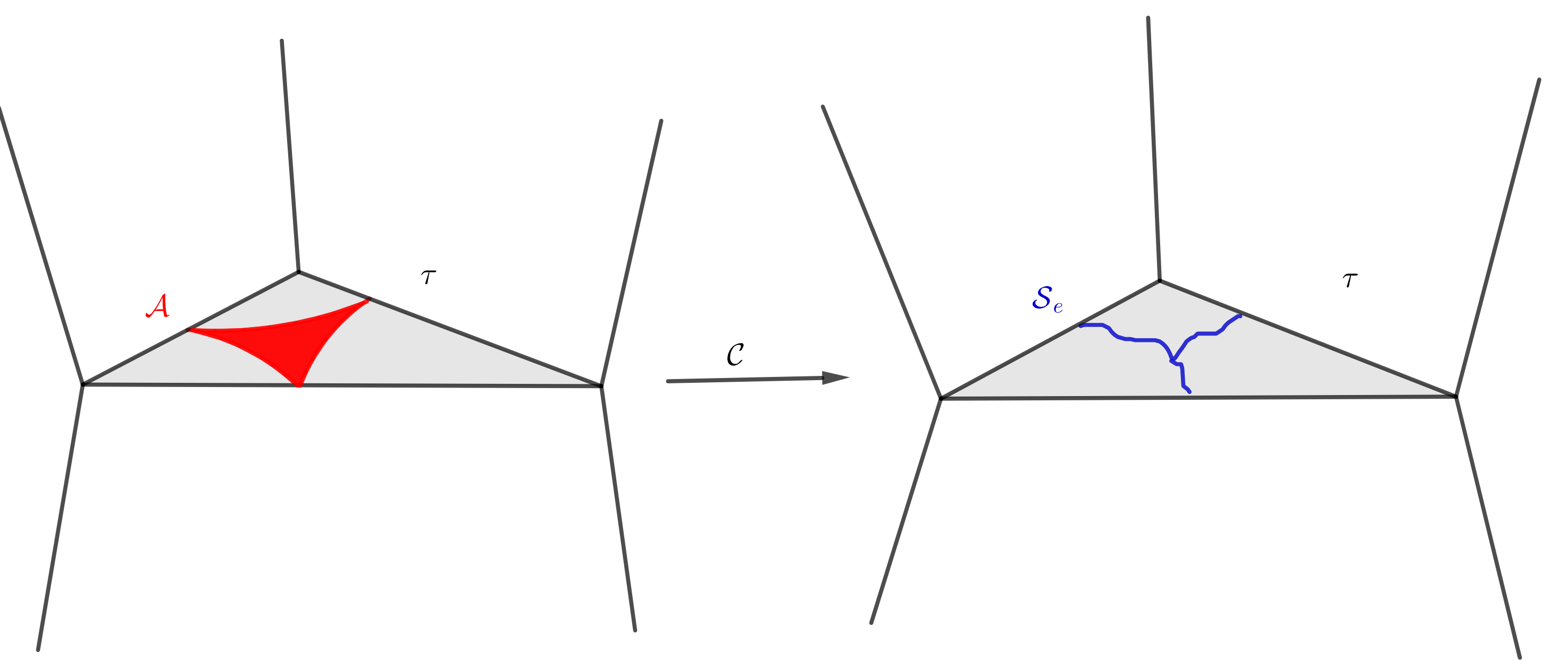
Figure 1. Contraction map $\mathscr{C}$

If $\mathcal{A}\cap\text{int}_{\text{re}}(\tau)\neq\emptyset$, it is given by the intersection of the zero locus $s_{v\tau}^{-1}(f_{v\rho})$ with $\mathbb{C}^{*}\cong V_{\tau}(\tau)\subset V(\tau)$. Taking $m$ to be the primitive vector in $\Lambda_{\tau}$ starting at $v$ that points into $\tau$, we can write $s_{v\tau}^{-1}(f_{v\rho})=1+s_{v\tau}^{-1}(m)z^{m}$. Taking the log map $\log:\mathbb{C}^{*}\rightarrow\real$, we see that $\log(\mathcal{A}\cap\text{int}_{\text{re}}(\tau))=c_{\tau}$. Therefore, for an edge $\tau\in\mathscr{P}^{[1]}$, we can define $\mathscr{C}$ to be the identity on $\tau$.

On a codimension $1$ cell $\rho$ such that $\text{int}_{\text{re}}(\rho)\cap\mathcal{A}\neq\emptyset$, we take the log map $\log:\text{Spec}_{\text{an}}(\mathbb{C}[\Lambda_{\rho}])\cong(\mathbb{C}^{*})^{2}\rightarrow\Lambda_{\rho,\real}^{*}\cong{}^{2}$ as shown in the Figure 2. We take a big enough polytope $\mathtt{P}$ (colored as purple) such that $\mathcal{A}\setminus\mathtt{P}$ is a disjoint union of legs. We contract the polytope $\mathtt{P}$ to the $0$-dimensional strata of $\mathscr{S}_{e}$. Each leg can be contracted to the tropical singular locus (colored as blue) along the normal direction to the tropical singular locus. Once it is constructed for all $\rho$, we can then extend it continuously to $B$ so that it is a diffeomorphism of $\text{int}_{\text{re}}(\sigma)$ for every maximal cell $\sigma$.

It is chosen such that the preimage $\mathscr{C}^{-1}(x)$ for every point $x\in\text{int}_{\text{re}}(\rho)$ is a convex polytope in ². Therefore, given any open subset $U\subset{}^{2}$ containing $\mathscr{C}^{-1}(x)$, we can find some convex open neighborhood $W_{1}\subset U$ of $\mathscr{C}^{-1}(x)$ giving the corresponding Stein open subset $\log^{-1}(W_{1})\subset(\mathbb{C}^{*})^{2}$. By taking $W=W_{1}\times W_{2}$ in the chart $\Lambda_{\rho,\real}^{*}\times\mathscr{Q}_{\rho,\real}$ as in the proof of Lemma 3.1, we have the open subset $W$ that satisfy condition (5) in Assumption 3.4.

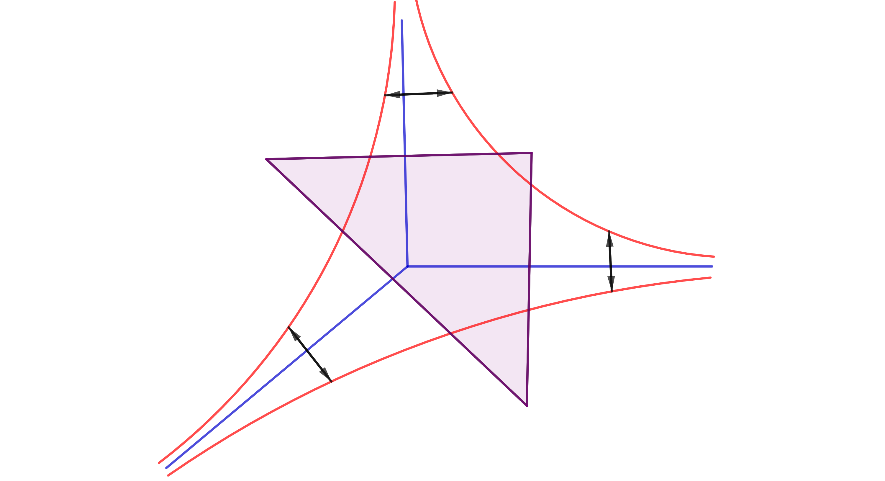
Figure 2. Contraction at $\rho$

In general, we need to construct $\mathscr{C}|_{\text{int}_{\text{re}}(\tau)}$ inductively for each $\tau\in\mathscr{P}$, such that the preimage $\mathscr{C}^{-1}(x)\subset\text{int}_{\text{re}}(\tau)$ is convex in the chart $\Lambda_{\tau,\real}^{*}\cong\text{int}_{\text{re}}(\tau)$ and the codimension $1$ amoeba $\mathcal{A}$ is contracted to the codimension $2$ tropical singular locus $\mathscr{S}_{e}$. The reason for introducing such a contraction map is that we can modify the generalized moment map $\mu$ to one which is more closely related with tropical geometry:

Definition 3.5.

We call the composition $\nu:=\mathscr{C}\circ\mu:\prescript{0}{}{X}\rightarrow B$ the modified moment map.

One immediate consequence of property $(4)$ in Assumption 3.4 is that we have $R\nu_{*}(\mathcal{F})=\nu_{*}(\mathcal{F})$ for any coherent sheaf $\mathcal{F}$ on $\prescript{0}{}{X}$, thanks to Lemma 3.1 and Cartan’s Theorem B:

Theorem 3.6 (Cartan’s Theorem B [4]; see e.g. Ch. IX, Cor. 4.11 in [11]).

For any coherent sheaf $\mathcal{F}$ over a Stein space $U$, we have $H^{>0}(U,\mathcal{F})=0.$

3.2.2. Monodromy invariant differential forms on $B$

Outside of the essential singular locus $\mathscr{S}_{e}$, we have a nice integral affine manifold $B\setminus\mathscr{S}_{e}$, on which we can talk about the sheaf $\Omega^{*}$ of (-valued) de Rham differential forms. But actually we can extend its definition to $\mathscr{S}_{e}$ using monodromy invariant differential forms.

We consider the inclusion $\iota:B_{0}:=B\setminus\mathscr{S}_{e}\rightarrow B$ and the natural exact sequence

(3.8) $$0\rightarrow\underline{\mathbb{Z}}\rightarrow\mathcal{A}\mathit{ff}\rightarrow\iota_{*}\Lambda_{B_{0}}^{*}\rightarrow 0,$$

where $\Lambda_{B_{0}}^{*}$ denotes the sheaf of integral cotangent vectors on $B_{0}$. For any $\tau\in\mathscr{P}$, the stalk $\Lambda_{B_{0},x}^{*}$ at a point $x\in\text{int}_{\text{re}}(\tau)\cap\mathscr{S}_{e}$ can be described using the chart $\Upsilon_{\tau}$ in (3.4). Using the description in §3.2, we have $x\in\mathscr{S}_{e,\tau,\rho}=\text{int}_{\text{re}}(\rho)\times\{o\}$ for some $\rho\in\mathtt{i}_{\tau}^{-1}(\mathscr{N}_{\Delta_{1}(\tau)}\times\cdots\times\mathscr{N}_{\Delta_{p}(\tau)})$. Taking a vertex $v\in\tau$ we can consider the monodromy transformations $T_{\gamma}$’s around the strata $\mathscr{S}_{e,\eta,\rho}$’s that contain $x$ in their closures. We can idenfity the stalk $\iota_{*}(\Lambda_{B_{0}}^{*})_{x}$ as the subset of $T_{v}^{*}$ that is invariant under all such monodromy transformations. Since $\rho\subset\Lambda_{\tau,\real}^{*}$ is a cone, we have $\Lambda_{\rho}\subset\Lambda_{\tau}^{*}$. Using the natural projection map $\pi_{v\tau}:T_{v}^{*}\rightarrow\Lambda_{\tau}^{*}$, we have the identification $\iota_{*}(\Lambda_{B_{0}}^{*})_{x}\cong\pi_{v\tau}^{-1}(\Lambda_{\rho})$. There is a direct sum decomposition $\iota_{*}(\Lambda_{B_{0}}^{*})_{x}=\Lambda_{\rho}\oplus\mathscr{Q}_{\tau}^{*}$, depending on a decomposition $T_{v}=\Lambda_{\tau}\oplus\mathscr{Q}_{\tau}$. This gives the map

(3.9) $$\mathtt{x}:U_{x}\rightarrow\pi_{v\tau}^{-1}(\Lambda_{\rho})^{*}$$

in a sufficiently small neighborhood $U_{x}$, locally defined up to a translation in $\pi_{v\tau}^{-1}(\Lambda_{\rho})^{*}$. We need to describe the compatibility between the map associated to a point $x\in\mathscr{S}_{e,\omega,\rho}$ and that to a point $\tilde{x}\in\mathscr{S}_{e,\tau,\tilde{\rho}}$ such that $\mathscr{S}_{e,\omega,\rho}\subset\overline{\mathscr{S}_{e,\tau,\tilde{\rho}}}$.

This first case is when $\omega=\tau$. We let $\tilde{x}\in\text{int}_{\text{re}}(\tilde{\rho})\times\{o\}\cap U_{x}$ for some $\rho\subset\tilde{\rho}$. Then, after choosing suitable translations in $\pi_{v\tau}^{-1}(\Lambda_{\rho})^{*}$ for the maps $\mathtt{x}$ and $\tilde{\mathtt{x}}$, we have the following commutative diagram:

(3.10)

The second case is when $\omega\subsetneq\tau$. Making use of the change $\gimel$ of charts in equation (3.5), and the description in the proof of Lemma 3.3, we write $\tilde{x}\in\text{int}_{\text{re}}(\tilde{\rho})\times\{o\}$ for some cone $\tilde{\rho}=\mathtt{i}_{\tau}^{-1}(\prod_{j=1}^{p}\tilde{\rho}_{j})\in\mathtt{i}_{\tau}^{-1}\big{(}\prod_{j=1}^{p}\Lambda_{\Delta_{j}(\tau)}^{*}\big{)}$ with positive codimension. In $\gimel^{-1}(W)$, we may assume $\tilde{\rho}$ is the pullback of a cone $\breve{\rho}$ via $\Pi_{\omega\subset\tau}\circ\mathtt{p}_{\tau}$ as in equation (3.7). Since $\mathscr{S}_{e,\omega,\rho}\subset\overline{\mathscr{S}_{e,\tau,\tilde{\rho}}}$, we have $\rho\subset\mathtt{p}_{\omega}^{-1}(\breve{\rho})$ and hence $\mathtt{p}_{\omega\subset\tau}^{-1}(\Lambda_{\rho})\subset\Lambda_{\tilde{\rho}}$. Therefore, from $\mathtt{p}_{\omega\subset\tau}\circ\pi_{v\tau}=\pi_{v\omega}$, we obtain $\pi_{v\omega}^{-1}(\Lambda_{\rho})\subset\pi_{v\tau}^{-1}(\Lambda_{\tilde{\rho}})$ inducing the map $\mathtt{p}:\pi_{v\tau}^{-1}(\Lambda_{\tilde{\rho}})^{*}\rightarrow\pi_{v\omega}^{-1}(\Lambda_{\rho})^{*}$. As a result, we still have the above commutative diagram (3.10) for a point $\tilde{x}$ sufficiently close to $x$.

Definition 3.7.

Given $x\in\mathscr{S}_{e}$ as above, the stalk of $\Omega^{*}$ at $x$ is defined as $\Omega^{*}_{x}:=(\mathtt{x}^{-1}\Omega^{*})_{x}$, which is equipped with the de Rham differential $d$. This defines the complex $(\Omega^{*},d)$ (or simply $\Omega^{*}$) of monodromy invariant differential forms on $B$. A section $\alpha\in\Omega^{*}(W)$ is a collection of elements $\alpha_{x}\in\Omega^{*}_{x}$, $x\in W$ such that each $\alpha_{x}$ can be represented by $\mathtt{x}^{-1}\beta_{x}$ in a small neighborhood $U_{x}\subset\mathtt{p}^{-1}(\mathtt{U}_{x})$ for some smooth form $\beta_{x}$ on $\mathtt{U}_{x}$, and satisfies the relation $\alpha_{\tilde{x}}=\tilde{\mathtt{x}}^{-1}(\mathtt{p}^{*}\beta_{x})$ in $\Omega^{*}_{\tilde{x}}$ for every $\tilde{x}\in U_{x}$.

It follows from the definition that $\underline{\real}\rightarrow\Omega^{*}$ is a resolution. We shall also prove the existence of a partition of unity.

Lemma 3.8.

Given any $x\in B$ and a sufficiently small neighborhood $U$, there exists $\varrho\in\Omega^{0}(U)$ with compact support in $U$ such that $0\leq\varrho\leq 1$ and $\varrho\equiv 1$ near $x$. (Since $\Omega^{0}$ is a subsheaf of the sheaf $\mathcal{C}^{0}$ of continuous functions on $B$, we can talk about the value $f(x)$ for $f\in\Omega^{0}(W)$ and $x\in W$.)

Proof.

If $x\notin\mathscr{S}_{e}$, the statement is a standard fact. So we assume that $x\in\text{int}_{\text{re}}(\tau)\cap\mathscr{S}_{e}$ for some $\tau\in\mathscr{P}$. As above, we an write $x\in\text{int}_{\text{re}}(\rho)\times\{o\}$. Furthermore, since $\rho$ is a cone in the fan $\mathtt{i}_{\tau}^{-1}(\mathscr{N}_{\Delta_{1}(\tau)}\times\cdots\times\mathscr{N}_{\Delta_{p}(\tau)})$, $\Lambda_{\tau}^{*}$ has $\Lambda_{\Delta_{1}(\tau)}^{*}\oplus\cdots\oplus\Lambda_{\Delta_{p}(\tau)}^{*}$ as a direct summand, and the description of $\iota_{*}(\Lambda_{B_{0}}^{*})_{x}$ is compatible with the direct sum decomposition of $\Lambda_{\tau}^{*}$, we may further assume that $p=1$ and $\tau=\Delta_{1}(\tau)$ is a simplex.

If $\rho$ is not the smallest cone (i.e. the one consisting of just the origin in $\mathscr{N}_{\tau}$), we have a decomposition $\Lambda_{\tau}^{*}=\Lambda_{\rho}\oplus\mathscr{Q}_{\rho}$ with natural projection $\mathtt{p}:\Lambda_{\tau}^{*}\rightarrow\mathscr{Q}_{\rho}$. Then, locally near $x$, we can write the normal fan $\mathscr{N}_{\tau}$ as $\mathtt{p}^{-1}(\Sigma_{\rho})$ for some normal fan $\Sigma_{\rho}\subset\mathscr{Q}_{\rho}$ of a lower dimensional simplex. So we are reduced to the case when $\rho=\{o\}$ is the smallest cone in the fan $\mathscr{N}_{\tau}$.

Now we construct the function $\varrho$ near the origin $o\in\mathscr{N}_{\tau}$ by induction on the dimension of the fan $\mathscr{N}_{\tau}$ When $\dim(\mathscr{N}_{\tau})=1$, it is the fan of $\mathbb{P}^{1}$ with three cones _-, $\{o\}$ and ₊. One can construct the bump function which is equal to $1$ near $o$ and supported in a sufficiently small neighborhood of $o$. For the induction step, we consider an $n$-dimensional fan $\mathscr{N}_{\tau}$. For any point $x$ near but not equal to $o$, we have $x\in\text{int}_{\text{re}}(\rho)$ for some $\rho\neq\{o\}$. Then we can decompose $\mathscr{N}_{\tau}$ locally as $\Lambda_{\rho}\oplus\mathscr{Q}_{\rho}$. Applying the induction hypothesis to $\mathscr{Q}_{\rho}$ gives us a bump function $\varrho_{x}$ compactly supported in any sufficiently small neighborhood of $x$ (for the $\Lambda_{\rho}$ directions, we do not need the induction hypothesis to get the bump function). This produces a partition of unity $\{\varrho_{i}\}$ outside $o$. Finally, letting $\varrho:=1-\sum_{i}\varrho_{i}$ and extending it continuously to the origin $o$ gives the desired function. ∎

Lemma 3.8 produces a partition of unity for the complex $(\Omega^{*},d)$ of monodromy invariant differential forms on $B$ to satisfy the requirement in Condition 4.7 below. In particular, the cohomology of $(\Omega^{*}(B),d)$ computes $R\Gamma(B,\underline{\real})$. Given a point $x\in B\setminus\mathscr{S}_{e}$, we take an element $\varrho_{x}\in\Omega^{n}(B)$ which is compactly supported in an arbitrary small neighborhood $U_{x}\subset B\setminus\mathscr{S}_{e}$, representing a non-zero element in the cohomology $H^{n}(\Omega^{*},d)=H^{n}(B,\mathbb{C})\cong\mathbb{C}$.

4. Smoothing of maximally degenerate Calabi-Yau varieties via dgBV algebras

In this section, we review and refine the results in [5] concerning smoothing of the maximally degenerate Calabi-Yau log variety $\prescript{0}{}{X}^{\dagger}$ over $\hat{S}^{\dagger}=\text{Spec}_{\text{an}}(\hat{R})^{\dagger}=\text{Spec}_{\text{an}}(\mathbb{C}[[q]])^{\dagger}$ using the local smoothing models $V^{\dagger}\rightarrow\prescript{k}{}{\mathbb{V}}^{\dagger}$’s specified in §2.4. In order to relate with tropical geometry on $B$, we will choose $V$ so that it is the pre-image $\nu^{-1}(W)$ of an open subset $W$ in $B$.

4.1. Good covers and local smoothing data

Given $\tau\in\mathscr{P}$ and a point $x\in\text{int}_{\text{re}}(\tau)\subset B$, we take a sufficiently small open subset $W\in\mathscr{B}_{x}$. We need to construct a local smoothing model on $V=\nu^{-1}(W)$.

• If $x\notin\mathscr{S}$, then we can simply take the local smoothing $\prescript{}{}{\mathbb{V}}^{\dagger}$ introduced in (2.14) in §2.4.

• If $x\in\mathscr{S}$, we assume that $\mathscr{C}^{-1}(W)\cap\mathcal{A}^{\tau}_{i}\neq\emptyset$ for $i=1,\dots,r$, and take $\psi_{x,i}=\psi_{i}$ for $1\leq i\leq r$ and $\psi_{x,i}=0$ otherwise accordingly. Then we can take $P_{\tau,x}$ introduced in (2.17) and the map $V=\nu^{-1}(W)\rightarrow\text{Spec}_{\text{an}}(\mathbb{C}[\Sigma_{\tau}\oplus\mathbb{Z}^{l}])$ described in §2.4. By shrinking $W$, if necessary, one can show that it is an embedding using an argument similar to [19, Thm. 2.6].

Condition 4.1.

An open cover $\{W_{\alpha}\}_{\alpha}$ of $B$ is said to be good if

1. for each $W_{\alpha}$, there exists a unique $\tau_{\alpha}\in\mathscr{P}$ such that $W_{\alpha}\in\mathscr{B}_{x}$ for some $x\in\text{int}_{\text{re}}(\tau)$;

2. $W_{\alpha\beta}=W_{\alpha}\cap W_{\beta}\neq\emptyset$ only when $\tau_{\alpha}\subset\tau_{\beta}$ or $\tau_{\beta}\subset\tau_{\alpha}$, and if this is the case, we have either $\text{int}_{\text{re}}(\alpha)\cap W_{\alpha\beta}\neq\emptyset$ or $\text{int}_{\text{re}}(\beta)\cap W_{\alpha\beta}\neq\emptyset$.

Given a good cover $\{W_{\alpha}\}_{\alpha}$ of $B$, we have the corresponding Stein open cover $\mathcal{V}=\{V_{\alpha}\}_{\alpha}$ of $\prescript{0}{}{X}$ given by $V_{\alpha}:=\nu^{-1}(W_{\alpha})$ for each $\alpha$. For each $V_{\alpha}^{\dagger}$, the infinitesimal local smoothing model is given as a log space $\prescript{}{}{\mathbb{V}}_{\alpha}^{\dagger}$ over $\hat{S}^{\dagger}$ (see (2.14)). Let $\prescript{k}{}{\mathbb{V}}_{\alpha}$ be the $k^{\text{th}}$-order thickening over $\prescript{k}{}{S}^{\dagger}=\text{Spec}_{\text{an}}(R/\mathbf{m}^{k+1})^{\dagger}$ and $j:V_{\alpha}\setminus Z\hookrightarrow V_{\alpha}$ be the open inclusion. As in [5, §8], we obtain coherent sheaves of BV algebras (and modules) over $V_{\alpha}$ from these local smoothing models. But for the purpose of this paper, we would like to push forward these coherent sheaves to $B$ and work on the open subsets $W_{\alpha}$’s. This leads to the following modification of [5, Def. 7.6] (see also [5, Def. 2.14 and 2.20]):

Definition 4.2.

For each $k\in\mathbb{Z}_{\geq 0}$, we define

• the sheaf of $k^{\text{th}}$-order polyvector fields to be $\prescript{k}{}{\mathcal{G}}_{\alpha}^{*}:=\nu_{*}j_{*}(\bigwedge^{-*}\Theta_{\prescript{k}{}{\mathbb{V}}_{\alpha}^{\dagger}/\prescript{k}{}{S}^{\dagger}})$ (i.e. push-forward of relative log polyvector fields on $\prescript{k}{}{\mathbb{V}}_{\alpha}^{\dagger}$);

• the $k^{\text{th}}$-order log de Rham complex to be $\prescript{k}{}{\mathcal{K}}^{*}_{\alpha}:=\nu_{*}j_{*}(\Omega^{*}_{\prescript{k}{}{\mathbb{V}}_{\alpha}^{\dagger}/\mathbb{C}})$ (i.e. push-forward of log de Rham differentials) equipped with the de Rham differential $\prescript{k}{}{\partial}_{\alpha}=\prescript{}{}{\partial}$ which is naturally a dg module over $\prescript{k}{}{\Omega}^{*}_{S^{\dagger}}$;

• the local log volume form $\prescript{}{}{\omega}_{\alpha}$ as a nowhere vanishing element in $\nu_{*}j_{*}(\Omega^{n}_{\prescript{}{}{\mathbb{V}}_{\alpha}^{\dagger}/\hat{S}^{\dagger}})$ and the $k^{\text{th}}$-order volume form to be $\prescript{k}{}{\omega}_{\alpha}=\prescript{}{}{\omega}_{\alpha}\ (\text{mod $\mathbf{m}^{k+1}$})$.

A natural filtration $\prescript{k}{\bullet}{\mathcal{K}}^{*}_{\alpha}$ is given by $\prescript{k}{s}{\mathcal{K}}^{*}_{\alpha}:=\prescript{k}{}{\Omega}^{\geq s}_{S^{\dagger}}\wedge\prescript{k}{}{\mathcal{K}}^{*}_{\alpha}[s]$ and taking wedge product defines the natural sheaf isomorphism $\prescript{k}{r}{\sigma}^{-1}:\prescript{k}{}{\Omega}^{r}_{S^{\dagger}}\otimes_{\prescript{k}{}{R}}(\prescript{k}{0}{\mathcal{K}}^{*}_{\alpha}/\prescript{k}{1}{\mathcal{K}}^{*}_{\alpha}[-r])\rightarrow\prescript{k}{r}{\mathcal{K}}^{*}_{\alpha}/\prescript{k}{r+1}{\mathcal{K}}^{*}_{\alpha}$. We have the space $\prescript{k}{\parallel}{\mathcal{K}}^{*}_{\alpha}:=\prescript{k}{0}{\mathcal{K}}^{*}_{\alpha}/\prescript{k}{1}{\mathcal{K}}^{*}_{\alpha}\cong\nu_{*}j_{*}(\Omega^{*}_{\prescript{k}{}{\mathbf{V}}_{\alpha}^{\dagger}/\prescript{k}{}{S}^{\dagger}})$ of relative log de Rham differentials.

There is a natural action $v\lrcorner\varphi$ for $v\in\prescript{k}{}{\mathcal{G}}_{\alpha}^{*}$ and $\varphi\in\prescript{k}{}{\mathcal{K}}^{*}$ given by contracting a logarithmic holomorphic vector fields $v$ with a logarithmic holomorphic form $\varphi$. We define the Lie derivative via the formula $(-1)^{|v|}\mathcal{L}_{v}:=[\prescript{}{}{\partial},v\lrcorner]$. By contracting with $\prescript{k}{}{\omega}_{\alpha}$, we get a sheaf isomorphism $\lrcorner\prescript{k}{}{\omega}_{\alpha}:\prescript{k}{}{\mathcal{G}}_{\alpha}^{*}\rightarrow\prescript{k}{\parallel}{\mathcal{K}}^{*}_{\alpha}$, which defines the BV operator $\prescript{k}{}{\Delta}_{\alpha}$ by $\prescript{k}{}{\Delta}_{\alpha}(\varphi)\lrcorner\prescript{k}{}{\omega}:=\prescript{k}{}{\partial}_{\alpha}(\varphi\lrcorner\prescript{k}{}{\omega})$. We call it the BV operator because it satisfies the BV identity

(4.1) $$(-1)^{|v|}[v,w]:=\Delta(v\wedge w)-\Delta(v)\wedge w-(-1)^{|v|}v\wedge\Delta(w)$$

for $v,w\in\prescript{k}{}{\mathcal{G}}_{\alpha}^{*}$ if we put $\Delta=\prescript{k}{}{\Delta}_{\alpha}$. This gives $\prescript{k}{}{\mathcal{G}}^{*}_{\alpha}$ the structure of a sheaf of BV algebras.

4.2. An explicit description of the sheaf of log de Rham forms

Here we apply the calculations in [19, 14] to give an explicit description of the stalk $\prescript{k}{}{\mathcal{K}}_{\alpha,x}^{*}$.

Let us consider $K=\nu^{-1}(x)$ and the local model near $K$ described in §4.1, with $P_{\tau,x}$ and $Q_{\tau,x}$ as in (2.17) and an embedding $V\rightarrow\text{Spec}_{\text{an}}(\mathbb{C}[Q_{\tau,x}])$. We may treat $K\subset V$ as a compact subset of $\mathbb{C}^{l}=\text{Spec}_{\text{an}}(\mathbb{C}[\mathbb{N}^{l}])\hookrightarrow\text{Spec}_{\text{an}}(\mathbb{C}[Q_{\tau,x}])$ via the identification $\text{Spec}_{\text{an}}(\mathbb{C}[\Sigma_{\tau}\oplus\mathbb{N}^{l}])\cong\text{Spec}_{\text{an}}(\mathbb{C}[Q_{\tau,x}])$. For each $m\in\Sigma_{\tau}$, we denote the corresponding element $(m,\psi_{x,0}(m),\dots,\psi_{x,l}(m))\in P_{\tau,x}$ by $\hat{m}$ to avoid any confusion, and the corresponding function by $z^{\hat{m}}\in\mathbb{C}[P_{\tau,x}]$. Similar to [14, Lem. 7.14], the germ of holomorphic functions $\mathcal{O}_{\prescript{k}{}{\mathbb{V}},K}$ near $K$ in the space $\prescript{k}{}{\mathbb{V}}=\text{Spec}_{\text{an}}(\mathbb{C}[P_{\tau,x}/q^{k+1}])$ can be written as

(4.2) $$\mathcal{O}_{\prescript{k}{}{\mathbb{V}},K}=\Bigg{\{}\sum_{m\in\Sigma_{\tau},\ 0\leq i\leq k}\alpha_{m,i}q^{i}z^{\hat{m}}\,\Big{|}\,\alpha_{m,i}\in\mathcal{O}_{\mathbb{C}^{l}}(U)\ \text{for some neigh. $U\supset K$},\ \sup_{m\in\Sigma_{\tau}\setminus\{0\}}\frac{\log|\alpha_{m,i}|}{\mathtt{d}(m)}<\infty\Bigg{\}},$$

where $\mathtt{d}:\Sigma_{\tau}\rightarrow\mathbb{N}$ is a monoid morphism such that $\mathtt{d}^{-1}(0)=0$, and it is equipped with the product $z^{\hat{m}_{1}}\cdot z^{\hat{m}_{2}}:=z^{\hat{m}_{1}+\hat{m}_{2}}$ (but note that $\widehat{m_{1}+m_{2}}\neq\hat{m}_{2}+\hat{m}_{2}$ in general). Thus we have $\prescript{k}{}{\mathcal{K}}^{0}_{\alpha,x}\cong\prescript{k}{}{\mathcal{G}}_{\alpha,x}^{0}\cong\mathcal{O}_{\prescript{k}{}{\mathbb{V}},K}$.

To describe differential forms, we consider the vector space $\mathscr{E}=P_{\tau,x,\mathbb{C}}$, regarded as $1$-forms on $\text{Spec}_{\text{an}}(\mathbb{C}[P_{\tau,x}^{\text{gp}}])\cong(\mathbb{C}^{*})^{n+1}$. Write $d\log z^{p}$ for $p\in P_{\tau,x,\mathbb{C}}$ and set $\mathscr{E}_{1}:=\mathbb{C}\langle d\log u_{i}\rangle_{i=1}^{l}$, as a subset of $\mathscr{E}$. For an element $m\in\mathscr{Q}_{\tau,\mathbb{C}}$, we have the corresponding $1$-form $d\log z^{\hat{m}}\in P_{\tau,x,\mathbb{C}}$ under the association between $m$ and $z^{\hat{m}}$. Let $\mathtt{P}$ be the power set of $\{1,\dots,l\}$ and write $u^{I}=\prod_{i\in I}u_{i}$ for $I\in\mathtt{P}$. A computation for sections of the sheaf $j_{*}(\Omega^{r}_{\prescript{k}{}{\mathbb{V}}^{\dagger}/\mathbb{C}})$ from [19, Prop. 1.12] and [14, Lem. 7.14] can then be rephrased as the following lemma.

Lemma 4.3 ([19, 14]).

The germ of sections of $j_{*}(\Omega^{*}_{\prescript{k}{}{\mathbb{V}}^{\dagger}/\mathbb{C}})_{K}$ near $K$ is a subspace of $\mathcal{O}_{\prescript{k}{}{\mathbb{V}},K}\otimes\bigwedge^{*}\mathscr{E}$ given by elements of the form

$$\alpha=\sum_{\begin{subarray}{c}m\in\Sigma_{\tau}\\ 0\leq i\leq k\end{subarray}}\sum_{I}\alpha_{m,i,I}q^{i}z^{\hat{m}}u^{I}\otimes\beta_{m,I},\quad\beta_{m,I}\in\bigwedge\nolimits^{*}\mathscr{E}_{m,I}=\bigwedge\nolimits^{*}(\mathscr{E}_{1,m,I}\oplus\mathscr{E}_{2,m,I}\oplus\langle d\log q\rangle),$$

where $\mathscr{E}_{1,m,I}=\langle d\log u_{i}\rangle_{i\in I}\subset\mathscr{E}_{1}$ and the subspace $\mathscr{E}_{2,m,I}\subset\mathscr{E}$ is given as follows: we consider the pullback of the product of normal fans $\prod_{i\notin I}\mathscr{N}_{\check{\Delta}_{i}(\tau)}$ to $\mathscr{Q}_{\tau,\real}$ and take $\mathscr{E}_{2,m,I}=\langle d\log z^{\hat{m}^{\prime}}\rangle$ for $m^{\prime}\in\sigma_{m,I}$, where $\sigma_{m,I}$ is the smallest cone in $\prod_{i\notin I}\mathscr{N}_{\check{\Delta}_{i}(\tau)}\subset\mathscr{Q}_{\tau,\real}$ containing $m$.

Here we can treat $\prod_{i\notin I}\mathscr{N}_{\check{\Delta}_{i}(\tau)}\subset\mathscr{Q}_{\tau,\real}$ since $\bigoplus_{i}\Lambda_{\check{\Delta}_{i}(\tau)}$ is a direct summand of $\mathscr{Q}_{\tau}^{*}$. A similar description for $j_{*}(\Omega^{*}_{\prescript{k}{}{\mathbb{V}}^{\dagger}/\mathbb{C}^{\dagger}})_{K}$ is simply given by quotienting out the direct summand $\langle d\log q\rangle$ in the above formula for $\alpha$. In particular, if we restrict ourselves to the case $k=0$, a general element $\alpha$ can be written as

$$\alpha=\sum_{m\in\Sigma_{\tau}}\sum_{I}\alpha_{m,I}z^{\hat{m}}u^{I}\otimes\beta_{m,I},\quad\beta_{m,I}\in\bigwedge\nolimits^{*}\mathscr{E}_{m,I}=\bigwedge\nolimits^{*}(\mathscr{E}_{1,m,I}\oplus\mathscr{E}_{2,m,I}).$$

One can choose a nowhere vanishing element $\Omega=du_{1}\cdots du_{l}\otimes\eta\in u_{1}\cdots u_{l}\otimes\wedge^{l}\mathscr{E}_{1}\otimes\wedge^{n-\dim(\tau)}\mathscr{E}_{2}\subset j_{*}(\Omega^{n}_{\prescript{0}{}{\mathbb{V}}^{\dagger}/\mathbb{C}^{\dagger}})_{K}$ for some nonzero element $\eta\in\wedge^{n-\dim(\tau)}\mathscr{E}_{2}$, which is well defined up to rescaling. Any element in $j_{*}(\Omega^{n}_{\prescript{0}{}{\mathbb{V}}^{\dagger}/\mathbb{C}^{\dagger}})_{K}$ can be written as $f\Omega$ for some $f=\sum_{m\in\Sigma_{\tau}}f_{m}z^{\hat{m}}\in\mathcal{O}_{\prescript{0}{}{\mathbb{V}},K}$.

Recall that the subset $K\subset\mathbb{C}^{l}$ is intersecting the singular locus $Z^{\tau}_{1},\dots,Z^{\tau}_{r}$ (as in §4.1), where $u_{i}$ is the coordinate function of $\mathbb{C}^{l}$ with simple zeros along $Z_{i}^{\tau}$ for $i=1,\dots,r$. There is a change of coordinates between a neighborhood of $K$ in $\mathbb{C}^{l}$ and that of $K$ in $(\mathbb{C}^{*})^{l}$ given by

$$\begin{cases}u_{i}\mapsto f_{v,i}|_{(\mathbb{C}^{*})^{l}}&\text{if }1\leq i\leq r;\\ u_{i}\mapsto z_{i}&\text{if }r<i\leq l.\end{cases}$$

Under the map $\log:(\mathbb{C}^{*})^{l}\rightarrow{}^{l}$, we have $K=\log^{-1}(\mathscr{C})$ for some connected compact subset $\mathscr{C}\subset{}^{l}$. In the coordinates $z_{1},\dots,z_{l}$, we find that $d\log z_{1}\cdots d\log z_{l}\otimes\eta$ can be written as $f\Omega$ near $K$ for some nowhere vanishing function $f\in\mathcal{O}_{\prescript{0}{}{\mathbb{V}},K}$.

Lemma 4.4.

When $K\cap Z=\emptyset$, i.e. $r=0$ in the above discussion. The top cohomology group $\mathcal{H}^{n}(j_{*}(\Omega^{n}_{\prescript{0}{}{\mathbb{V}}^{\dagger}/\mathbb{C}^{\dagger}})_{K},\prescript{}{}{\partial}):=j_{*}(\Omega^{n}_{\prescript{0}{}{\mathbb{V}}^{\dagger}/\mathbb{C}^{\dagger}})_{K}/\text{Im}(\prescript{}{}{\partial})$ is isomorphic to $\mathbb{C}$, which is generated by the element $d\log z_{1}\cdots d\log z_{l}\otimes\eta$.

Proof.

Given a general element $f\Omega$ as above, first observe that we can write $f=f_{0}+f_{+}$, where $f_{+}=\sum_{m\in\Sigma_{\tau}\setminus\{0\}}f_{m}z^{\hat{m}}$ and $f_{0}\in\mathcal{O}_{\mathbb{C}^{l},K}$. Take a basis $e_{1},\dots,e_{s}$ of $\mathscr{Q}_{\tau,\real}^{*}$, and also a partition $I_{1},\dots,I_{s}$ of the lattice points in $\Sigma_{\tau}\setminus\{0\}$ such that $\langle e_{j},m\rangle\neq 0$ for $m\in I_{j}$. Letting

$$\alpha=(-1)^{l}\sum_{j}\sum_{m\in I_{j}}\frac{f_{m}}{\langle e_{j},m\rangle}z^{\hat{m}}du_{1}\cdots du_{l}\otimes\iota_{e_{j}}\eta,$$

we have $\prescript{}{}{\partial}(\alpha)=f_{+}\Omega$. So we only need to consider elements of the form $f_{0}\Omega$. If $f_{0}\Omega=\prescript{}{}{\partial}(\alpha)$ for some $\alpha$, we may take $\alpha=\sum_{j}\alpha_{j}du_{1}\cdots\widehat{du_{j}}\cdots du_{l}\otimes\eta$ for some $\alpha_{j}\in\mathcal{O}_{\mathbb{C}^{l},K}$. Now this is equivalent to $f_{0}du_{1}\cdots du_{l}=\prescript{}{}{\partial}\big{(}\sum_{j}\alpha_{j}du_{1}\cdots\widehat{du_{j}}\cdots du_{l}\big{)}$ as forms in $\Omega^{l}_{\mathbb{C}^{l},K}$. This reduces the problem to $\mathbb{C}^{l}$.

Working in $(\mathbb{C}^{*})^{l}$ with coordinates $z_{i}$’s, we can write

$$\mathcal{O}_{(\mathbb{C}^{*})^{l},K}=\left\{\sum_{m\in\mathbb{Z}^{l}}a_{m}z^{m}\ \Big{|}\ \sum_{m\in\mathbb{Z}^{l}}|a_{m}|e^{\langle v,m\rangle}<\infty,\ \text{for all $v\in W$, for some open $W\supset\mathscr{C}$}\right\},$$

using the fact that $K$ is multi-circular. By writing $\Omega^{*}_{(\mathbb{C}^{*})^{l},K}=\mathcal{O}_{(\mathbb{C}^{*})^{l},K}\otimes\bigwedge^{*}\mathscr{F}_{1}$ with $\mathscr{F}_{1}=\langle d\log z_{i}\rangle_{i=1}^{l}$, we can see that any element can be represented as $cd\log z_{1}\cdots d\log z_{l}$ in the quotient $\Omega^{l}_{(\mathbb{C}^{*})^{l},K}/\text{Im}(\prescript{}{}{\partial})$, for some constant $c$. ∎

From this, we conclude that the top cohomology sheaf $\mathcal{H}^{n}(\prescript{0}{\parallel}{\mathcal{K}}^{*},\prescript{}{}{\partial})$ is isomorphic to the locally constant sheaf $\underline{\mathbb{C}}$ over $B\setminus\mathscr{S}_{e}$.

Lemma 4.5.

Consider $x\in W_{\alpha}\setminus\mathscr{S}_{e}$. For an element of the form $e^{f}(\prescript{k}{}{\omega}_{\alpha})$ in $\prescript{k}{\parallel}{\mathcal{K}}^{n}_{\alpha,x}$ with $f\in\prescript{k}{}{\mathcal{G}}^{0}_{\alpha,x}\cong\mathcal{O}_{\prescript{k}{}{\mathbb{V}}_{\alpha},x}$ satisfying $f\cong 0\text{(mod $\mathbf{m}$)}$, there exist $h(q)\in\prescript{k}{}{R}=\mathbb{C}[q]/(q^{k+1})$ and $v\in\prescript{k}{}{\mathcal{G}}^{-1}_{\alpha,x}$ with $h,v\cong 0\text{(mod $\mathbf{m}$)}$ such that

(4.3) $$e^{f}(\prescript{k}{}{\omega}_{\alpha})=e^{h}e^{\mathcal{L}_{v}}(\prescript{k}{}{\omega}_{\alpha})$$

in $\prescript{k}{\parallel}{\mathcal{K}}^{n}_{\alpha,x}$.

Proof.

To simplify notations in this proof, we will drop the subscript $\alpha$. We prove the first statement by induction on $k$. The initial case is trivial. Assuming that this has been done for the $(k-1)^{\text{st}}$-order, then, by taking an arbitrary lifting $\tilde{v}$ of $v$ to the $k^{\text{th}}$-order, we have

$$e^{-h+f+q^{k}\epsilon}(\prescript{k}{}{\omega})=e^{\mathcal{L}_{\tilde{v}}}(\prescript{k}{}{\omega})$$

for some $\epsilon\in\mathcal{O}_{\prescript{0}{}{\mathbb{V}}_{x}}$. By Lemmas 4.4 and 4.6, we have $\epsilon\prescript{0}{}{\omega}=c\prescript{0}{}{\omega}+\prescript{}{}{\partial}(\gamma)$ for some $\gamma$ and some suitable constant $c$. Letting $\theta\lrcorner(\prescript{0}{}{\omega})=\gamma$ and $\breve{v}=\tilde{v}+q^{k}\theta$, we have

$$e^{\mathcal{L}_{\breve{v}}}(\prescript{k}{}{\omega})=e^{\mathcal{L}_{v}}(\prescript{k}{}{\omega})-q^{k}\prescript{}{}{\partial}(\theta\lrcorner(\prescript{0}{}{\omega}))=e^{-h+f+cq^{k}}(\prescript{k}{}{\omega}).$$

By defining $\tilde{h}(q)=h(q)-cq^{k}$ in $\mathbb{C}[q]/(q^{k+1})$, we obtain the desired expression. ∎

Lemma 4.6.

The volume element $\prescript{0}{}{\omega}$ is non-zero in $\mathcal{H}^{n}(\prescript{0}{\parallel}{\mathcal{K}}^{*},\prescript{}{}{\partial})_{x}$ for every $x\in B$.

Proof.

We first consider the case when $x\in\text{int}_{\text{re}}(\sigma)$ for some maximal cell $\sigma\in\mathscr{P}^{[n]}$. The toric stratum $\prescript{0}{}{X}_{\sigma}$ associated to $\sigma$ is equipped with the natural divisorial log structure induced from its boundary divisor. Then the sheaf $\Omega^{*}_{\prescript{0}{}{X}_{\sigma}^{\dagger}/\mathbb{C}^{\dagger}}$ of log derivations for $\prescript{0}{}{X}^{\dagger}$ is isomorphic to $\bigwedge^{n}\Lambda_{\sigma}\otimes_{\mathbb{Z}}\mathcal{O}_{\prescript{0}{}{X}_{\sigma}}$. By [19, Lem. 3.12], we have $\prescript{0}{}{\omega}_{x}=c(\mu_{\sigma})_{\nu^{-1}(x)}$ in $\nu_{*}(\Omega^{n}_{\prescript{0}{}{X}_{\sigma}^{\dagger}/\mathbb{C}^{\dagger}})_{x}\cong\prescript{0}{\parallel}{\mathcal{K}}^{n}_{x}$, where $\mu_{\sigma}\in\bigwedge^{n}\Lambda_{\sigma,\mathbb{C}}$ is nowhere vanishing and $c$ is a non-zero constant $c$. Thus $\prescript{0}{}{X}|_{x}$ is non-zero in the cohomology as the same is true for $\mu_{\sigma}\in\nu_{*}(\Omega^{n}_{\prescript{0}{}{X}_{\sigma}^{\dagger}/\mathbb{C}^{\dagger}})_{x}$.

Next we consider a general point $x\in\text{int}_{\text{re}}(\tau)$. If the statement is not true, we will have $\prescript{0}{}{\omega}_{x}=\prescript{0}{}{\partial}(\alpha)$ for some $\alpha\in\prescript{0}{\parallel}{\mathcal{K}}^{n-1}_{x}$. Then there is an open neighborhood $U\supset\mathscr{C}^{-1}(x)$ such that this relation continues to hold. As $U\cap\text{int}_{\text{re}}(\sigma)\neq\emptyset$, for those maximal cells $\sigma$ which contain the point $x$, we can take a nearby point $y\in U\cap\text{int}_{\text{re}}(\sigma)$ and conclude that $c\mu_{\sigma}=\prescript{0}{}{\partial}(\alpha)$ in $\nu_{*}(\Omega^{n}_{\prescript{0}{}{X}_{\sigma}^{\dagger}/\mathbb{C}^{\dagger}})_{y}$. This contradicts the previous case. ∎

4.3. A global pre-dgBV algebra from gluing

One approach for smoothing $\prescript{0}{}{X}$ is to look for gluing morphisms $\prescript{k}{}{\psi}_{\alpha\beta}:\prescript{k}{}{\mathbb{V}}_{\alpha}^{\dagger}|_{V_{\alpha\beta}}\rightarrow\prescript{k}{}{\mathbb{V}}_{\beta}^{\dagger}|_{V_{\alpha\beta}}$ between the local smoothing models which satisfy the cocycle condition, from which one obtain a $k^{\text{th}}$-order thickening $\prescript{k}{}{X}$ over $\prescript{k}{}{S}^{\dagger}$. This was done by Kontsevich-Soibelman [24] (in 2d) and Gross-Siebert [20] (in general dimensions) using consistent scattering diagrams. If such gluing morphisms $\prescript{k}{}{\psi}_{\alpha\beta}$’s are available, one can certainly glue the global $k^{\text{th}}$-order sheaves $\prescript{k}{}{\mathcal{G}}^{*}$, $\prescript{k}{}{\mathcal{K}}^{*}$ and the volume form $\prescript{k}{}{\omega}$.

In [5], we instead took suitable dg-resolutions $\prescript{k}{}{PV}^{*,*}_{\alpha}:=\Omega^{*}(\prescript{k}{}{\mathcal{G}}_{\alpha}^{*})$’s of the sheaves $\prescript{k}{}{\mathcal{G}}_{\alpha}^{*}$’s (more precisely, we used the Thom-Whitney resolution in [5, §3]) to construct gluings $\prescript{k}{}{g}_{\alpha\beta}:\Omega^{*}(\prescript{k}{}{\mathcal{G}}_{\alpha}^{*})|_{V_{\alpha\beta}}\rightarrow\Omega^{*}(\prescript{k}{}{\mathcal{G}}_{\beta}^{*})|_{V_{\alpha\beta}}$ of sheaves which only preserve the Gerstenhaber algebra structure but not the differential. The key discovery in [5] was that, as the sheaves $\Omega^{*}(\prescript{k}{}{\mathcal{G}}_{\alpha}^{*})$’s are soft, such a gluing problem could be solved without any information from the complicated scattering diagrams. What we obtained is a pre-dgBV algebra $\prescript{k}{}{PV}^{*,*}(\prescript{}{}{X})$, in which the differential squares to zero only modulo $\mathbf{m}=(q)$. Using well-known algebraic techniques [35, 22], we can solve the Maurer-Cartan equation and construct the thickening $\prescript{k}{}{X}$. In this subsection, we will summarize the whole procedure, incorporating the nice reformulation by Felten [13] in terms of deformations of Gerstenhaber algebras.

To begin with, we assume the following condition holds:

Condition 4.7.

There is a sheaf $(\Omega^{*},d)$ of unital differential graded algebras (abbrev. as dga) (over or $\mathbb{C}$) over $B$, with degrees $0\leq*\leq L$ for some $L$, such that

• the natural inclusion $\underline{\real}\rightarrow\Omega^{*}$ (or $\underline{\mathbb{C}}\rightarrow\Omega^{*}$) of the locally constant sheaf (concentrated at degree $0$) gives a resolution, and

• for any open cover $\mathcal{U}=\{U_{i}\}_{i\in\mathcal{I}}$, there is a partition of unity subordinate to $\mathcal{U}$, i.e. we have $\{\rho_{i}\}_{i\in\mathcal{I}}$ with $\rho_{i}\in\Gamma(U_{i},\Omega^{0})$ and $\overline{\text{supp}(\rho_{i})}\subset U_{i}$ such that $\{\overline{\text{supp}(\rho_{i})}\}_{i}$ is locally finite and $\sum_{i}\rho_{i}\equiv 1$.

It is easy to construct such $\Omega^{*}$ and there are many natural choices. For instance, if $B$ is a smooth manifold, then we can simply take the usual de Rham complex on $B$. In §3.2.2, the sheaf of monodromy invariant differential forms we constructed using the (singular) integral affine structure on $B$ is another possible choice for $\Omega^{*}$ (with degrees $0\leq*\leq n$). Yet another variant, namely, the sheaf of monodromy invariant tropical differential forms will be constructed in §5.1; this links tropical geometry on $B$ with smoothing of the maximally degenerate Calabi-Yau variety $\prescript{0}{}{X}$.

Let us recall how to obtain a gluing of the dg resolutions of the sheaves $\prescript{k}{}{\mathcal{G}}_{\alpha}^{*}$ and $\prescript{k}{}{\mathcal{K}}_{\alpha}^{*}$ using any possible choice of such an $\Omega^{*}$.

Definition 4.8.

We define $\prescript{k}{}{PV}_{\alpha}^{*,*}=\Omega^{*}(\prescript{k}{}{\mathcal{G}}_{\alpha}^{*}):=\Omega^{*}|_{W_{\alpha}}\otimes\prescript{k}{}{\mathcal{G}}^{*}_{\alpha}$, which gives a sheaf of dgBV algebras over $W_{\alpha}$. The dgBV structure $(\wedge,\bar{\partial}_{\alpha},\prescript{}{}{\Delta}_{\alpha})$ is defined componentwise by

$$(\varphi\otimes v)\wedge(\psi\otimes w) :=(-1)^{|v||\psi|}(\varphi\wedge\psi)\otimes(v\wedge w),$$

$$\bar{\partial}_{\alpha}(\varphi\otimes v):=(d\varphi)\otimes v, \quad\prescript{}{}{\Delta}_{\alpha}(\varphi\otimes v):=(-1)^{|\varphi|}\varphi\otimes(\prescript{}{}{\Delta}v),$$

for $\varphi,\psi\in\Omega^{*}(U)$ and $v,w\in\prescript{k}{}{\mathcal{G}}_{\alpha}^{*}(U)$ for open subset $U\subset W_{\alpha}$.

Definition 4.9.

We define $\prescript{k}{}{\mathcal{A}}_{\alpha}^{*,*}=\Omega^{*}(\prescript{k}{}{\mathcal{K}}_{\alpha}^{*}):=\Omega^{*}|_{W_{\alpha}}\otimes\prescript{k}{}{\mathcal{K}}^{*}_{\alpha}$, which gives a sheaf of dgas over $W_{\alpha}$ equipped with the natural filtration $\prescript{k}{\bullet}{\mathcal{A}}_{\alpha}^{*,*}$ inherited from $\prescript{k}{\bullet}{\mathcal{K}}^{*}_{\alpha}$. The structures $(\wedge,\bar{\partial}_{\alpha},\prescript{}{}{\partial}_{\alpha})$ are defined componentwise by

$$(\varphi\otimes u)\wedge(\psi\otimes w) :=(-1)^{|v||\psi|}(\varphi\wedge\psi)\otimes(u\wedge w),$$

$$\bar{\partial}_{\alpha}(\varphi\otimes u):=(d\varphi)\otimes u, \quad\prescript{}{}{\partial}_{\alpha}(\varphi\otimes u)=(-1)^{|\varphi|}\varphi\otimes(\prescript{}{}{\partial}u),$$

for $\varphi,\psi\in\Omega^{*}(U)$ and $u,w\in\prescript{k}{}{\mathcal{K}}_{\alpha}^{*}(U)$ for open subset $U\subset W_{\alpha}$.

There is an action of $\prescript{k}{}{PV}_{\alpha}$ on $\prescript{k}{}{\mathcal{A}}_{\alpha}$ by contraction $\lrcorner$ defined by the formula

$$(\varphi\otimes v)\lrcorner(\psi\otimes w):=(-1)^{|v||\psi|}(\varphi\wedge\psi)\otimes(v\lrcorner w),$$

for $\varphi,\psi\in\Omega^{*}(U)$, $v\in\prescript{k}{}{\mathcal{G}}_{\alpha}^{*}(U)$ and $w\in\prescript{k}{}{\mathcal{K}}_{\alpha}^{*}(U)$ for open subset $U\subset W_{\alpha}$. Note that the local holomorphic volume form $\prescript{k}{}{\omega}_{\alpha}\in\prescript{k}{\parallel}{\mathcal{A}}_{\alpha}^{n,0}(W_{\alpha})$ satisfies $\bar{\partial}_{\alpha}(\prescript{k}{}{\omega}_{\alpha})=0$, and we have the identity $\prescript{k}{}{\partial}_{\alpha}(\phi\lrcorner\prescript{k}{}{\omega}_{\alpha})=\prescript{k}{}{\Delta}_{\alpha}(\phi)\lrcorner\prescript{k}{}{\omega}_{\alpha}$ of operators.

The next step is to consider gluing of the local sheaves $\prescript{k}{}{PV}_{\alpha}$’s for higher orders $k$. Similar constructions have been done in [5, 13] using the combinatorial Thom-Whitney resolution for the sheaves $\prescript{k}{}{\mathcal{G}}_{\alpha}$’s. We make suitable modifications of those arguments to fit into our current setting.

First, since $\prescript{k}{}{\mathbb{V}}^{\dagger}_{\alpha}|_{V_{\alpha\beta}}$ and $\prescript{k}{}{\mathbb{V}}^{\dagger}_{\beta}|_{V_{\alpha\beta}}$ are divisorial deformations (in the sense of [19, Def. 2.7]) of the intersection $V^{\dagger}_{\alpha\beta}:=V^{\dagger}_{\alpha}\cap V^{\dagger}_{\beta}$, we can use [19, Thm. 2.11] and the fact that $V_{\alpha\beta}$ is Stein to obtain an isomorphism $\prescript{k}{}{\psi}_{\alpha\beta}:\prescript{k}{}{\mathbb{V}}^{\dagger}_{\alpha}|_{V_{\alpha\beta}}\rightarrow\prescript{k}{}{\mathbb{V}}^{\dagger}_{\beta}|_{V_{\alpha\beta}}$ of divisorial deformations which induces the gluing morphism $\prescript{k}{}{\psi}_{\alpha\beta}:\prescript{k}{}{\mathcal{G}}_{\alpha}^{*}|_{W_{\alpha\beta}}\rightarrow\prescript{k}{}{\mathcal{G}}_{\beta}^{*}|_{W_{\alpha\beta}}$ that in turn gives $\prescript{k}{}{\psi}_{\alpha\beta}:\prescript{k}{}{PV}_{\alpha}|_{W_{\alpha\beta}}\rightarrow\prescript{k}{}{PV}_{\beta}|_{W_{\alpha\beta}}$.

Definition 4.10.

A $k^{\text{th}}$-order Gerstenhaber deformation of $\prescript{0}{}{PV}$ is a collection of gluing morphisms $\prescript{k}{}{g}_{\alpha\beta}:\prescript{k}{}{PV}_{\alpha}|_{W_{\alpha\beta}}\rightarrow\prescript{k}{}{PV}_{\beta}|_{W_{\alpha\beta}}$ of the form $\prescript{k}{}{g}_{\alpha\beta}=e^{[\vartheta_{\alpha\beta},\cdot]}\circ\prescript{k}{}{\psi}_{\alpha\beta}$ for some $\theta_{\alpha\beta}\in\prescript{k}{}{PV}_{\beta}^{-1,0}(W_{\alpha\beta})$ with $\theta_{\alpha\beta}\equiv 0\ (\text{mod $\mathbf{m}$})$, such that the cocycle condition $\prescript{k}{}{g}_{\gamma\alpha}\circ\prescript{k}{}{g}_{\beta\gamma}\circ\prescript{k}{}{g}_{\alpha\beta}=\text{id}$ is satisfied.

An isomorphism between two $k^{\text{th}}$-order Gerstenhaber deformations $\{\prescript{k}{}{g}_{\alpha\beta}\}_{\alpha\beta}$ and $\{\prescript{k}{}{g}_{\alpha\beta}^{\prime}\}_{\alpha\beta}$ is a collection of automorphisms $\prescript{k}{}{h}_{\alpha}:\prescript{k}{}{PV}_{\alpha}\rightarrow\prescript{k}{}{PV}_{\alpha}$ of the form $\prescript{k}{}{h}_{\alpha}=e^{[\mathbf{b}_{\alpha},\cdot]}$ for some $\mathtt{b}_{\alpha}\in\prescript{k}{}{PV}_{\alpha}^{-1,0}(W_{\alpha})$ with $\mathtt{b}_{\alpha}\equiv 0(\text{mod $\mathbf{m}$})$, such that $\prescript{k}{}{g}_{\alpha\beta}^{\prime}\circ\prescript{k}{}{h}_{\alpha}=\prescript{k}{}{h}_{\beta}\circ\prescript{k}{}{g}_{\alpha\beta}$.

A slight modification of [13, Lem. 6.6], with essentially the same proof, gives the following:

Proposition 4.11.

Given a $k^{\text{th}}$-order Gerstenhaber deformation $\{\prescript{k}{}{g}_{\alpha\beta}\}_{\alpha\beta}$, the obstruction to the existence of a lifting to a $(k+1)^{\text{st}}$-order deformation $\{\prescript{k+1}{}{g}_{\alpha\beta}\}_{\alpha\beta}$ lies in the Čech cohomology (with respect to the cover $\mathcal{W}:=\{W_{\alpha}\}_{\alpha}$)

$$\check{H}^{2}(\mathcal{W},\prescript{0}{}{PV}^{-1,0})\otimes(\mathbf{m}^{k+1}/\mathbf{m}^{k}).$$

The isomorphism classs of $(k+1)^{\text{st}}$-order liftings are in

$$\check{H}^{1}(\mathcal{W},\prescript{0}{}{PV}^{-1,0})\otimes(\mathbf{m}^{k+1}/\mathbf{m}^{k}).$$

Fixing a $(k+1)^{\text{st}}$-order lifting $\{\prescript{k+1}{}{g}_{\alpha\beta}\}_{\alpha\beta}$, the automorphisms fixing $\{\prescript{k}{}{g}_{\alpha\beta}\}_{\alpha\beta}$ are in

$$\check{H}^{0}(\mathcal{W},\prescript{0}{}{PV}^{-1,0})\otimes(\mathbf{m}^{k+1}/\mathbf{m}^{k}).$$

Since $\Omega^{i}$ satisfies Condition 4.7, we have $\check{H}^{>0}(\mathcal{W},\prescript{0}{}{PV}^{-1,0})=0$. In particular, we always have a set of compatible Gerstenhaber deformations $\prescript{}{}{g}=(\prescript{k}{}{g})_{k\in\mathbb{N}}$ where $\prescript{k}{}{g}=\{\prescript{k}{}{g}_{\alpha\beta}\}_{\alpha\beta}$ and any two of them are equivalent. Fixing such a set $\prescript{}{}{g}$, we obtain a set $\{\prescript{k}{}{PV}\}_{k\in\mathbb{N}}$ of Gerstenhaber algebras which is compatible, in the sense that there are natural identifications $\prescript{k+1}{}{PV}\otimes_{\prescript{k+1}{}{R}}\prescript{k}{}{R}=\prescript{k}{}{PV}$.

We can also glue the local sheaves $\prescript{k}{}{\mathcal{A}}^{*}_{\alpha}$’s of dgas using $\prescript{}{}{g}$. First we can define $\prescript{k}{}{\psi}_{\alpha\beta}:\prescript{k}{}{\mathcal{K}}_{\alpha}^{*}|_{W_{\alpha\beta}}\rightarrow\prescript{k}{}{\mathcal{K}}_{\beta}^{*}|_{W_{\alpha\beta}}$ using $\prescript{k}{}{\psi}_{\alpha\beta}:\prescript{k}{}{\mathbb{V}}^{\dagger}_{\alpha}|_{V_{\alpha\beta}}\rightarrow\prescript{k}{}{\mathbb{V}}^{\dagger}_{\beta}|_{V_{\alpha\beta}}$. For each fixed $k$ we can write $\prescript{k}{}{g}_{\alpha\beta}=e^{[\vartheta_{\alpha\beta},\cdot]}\circ\prescript{k}{}{\psi}_{\alpha\beta}$ as before. Then

(4.4) $$\prescript{k}{}{g}:=e^{\mathcal{L}_{\vartheta_{\alpha\beta}}}\circ\prescript{k}{}{\psi}_{\alpha\beta}:\prescript{k}{}{\mathcal{A}}_{\alpha}^{*}|_{W_{\alpha\beta}}\rightarrow\prescript{k}{}{\mathcal{A}}_{\beta}^{*}|_{W_{\alpha\beta}}$$

preserves the dga structure $(\wedge,\prescript{}{}{\partial}_{\alpha})$ and the filtration on $\prescript{k}{\bullet}{\mathcal{A}}_{\alpha}^{*}$’s. As a result, we obtain a set of compatible sheaves $\{(\prescript{k}{}{\mathcal{A}}^{*},\wedge,\prescript{}{}{\partial})\}_{k\in\mathbb{N}}$ of dgas. The contraction action $\lrcorner$ is also compatible with the gluing construction so we have a natural action $\lrcorner$ of $\prescript{k}{}{PV}^{*}$ on $\prescript{k}{}{\mathcal{A}}^{*}$.

Next, we glue the operators $\bar{\partial}_{\alpha}$’s and $\prescript{}{}{\Delta}_{\alpha}$’s.

Definition 4.12.

A $k^{\text{th}}$-order predifferential $\bar{\partial}$ on $\prescript{k}{}{PV}^{*}$is a degree $1$ operator given by a collection of elements $\eta_{\alpha}\in\prescript{k}{}{PV}^{-1,1}_{\alpha}(W_{\alpha})$ such that $\eta_{\alpha}\equiv 0\ (\text{mod $\mathbf{m}$})$ and

$$\prescript{k}{}{g}_{\beta\alpha}\circ(\bar{\partial}_{\beta}+[\eta_{\beta},\cdot])\circ\prescript{k}{}{g}_{\alpha\beta}=(\bar{\partial}_{\alpha}+[\eta_{\alpha},\cdot]).$$

Two predifferentials $\bar{\partial}$ and $\bar{\partial}^{\prime}$ are equivalent if there is a Gerstenhaber automorphism (for the deformation $\prescript{k}{}{g}$) $h:\prescript{k}{}{PV}^{*}\rightarrow\prescript{k}{}{PV}^{*}$ such that $h^{-1}\circ\bar{\partial}\circ h=\bar{\partial}^{\prime}$.

Notice that we only have $\bar{\partial}^{2}\equiv 0$ $(\text{mod $\mathbf{m}$})$, which is why we call it a predifferential. Using the argument in [5, Thm. 3.34] or [13, Lem. 8.1], we can always lift any $k^{\text{th}}$-order predifferential $\prescript{k}{}{\bar{\partial}}$ to a $(k+1)^{\text{st}}$-order predifferential, and any two such liftings differ by a global element $\mathfrak{d}\in\prescript{0}{}{PV}^{-1,1}\otimes\mathbf{m}^{k+1}/\mathbf{m}^{k}$. We fix a set $\bar{\partial}:=\{\prescript{k}{}{\bar{\partial}}\}_{k\in\mathbb{N}}$ of such compatible predifferentials. For each $k$, the action of $\prescript{k}{}{\bar{\partial}}$ on $\prescript{k}{}{\mathcal{A}}^{*}$ is given by gluing of the action of $\bar{\partial}_{\alpha}+\mathcal{L}_{\eta_{\alpha}}$ on $\prescript{k}{}{\mathcal{A}}^{*}_{\alpha}$. On the other hand, the elements

(4.5) $$\mathfrak{l}_{\alpha}:=\bar{\partial}_{\alpha}(\eta_{\alpha})+\frac{1}{2}[\eta_{\alpha},\eta_{\alpha}]\in\prescript{k}{}{PV}^{-1,2}_{\alpha}(W_{\alpha})$$

glue to give a global element $\mathfrak{l}\in\prescript{k}{}{PV}^{-1,2}(B)$, and for different $k$’s, these elements are compatible. Computation shows that $\bar{\partial}^{2}=[\mathfrak{l},\cdot]$ on $\prescript{k}{}{PV}^{*}$ and $\bar{\partial}^{2}=\mathcal{L}_{\mathfrak{l}}$ on $\prescript{k}{}{\mathcal{A}}^{*}$.

To glue the operators $\prescript{}{}{\Delta}_{\alpha}$, we need to glue the local volume elements $\prescript{k}{}{\omega}_{\alpha}$’s to a global $\prescript{k}{}{\omega}$. We consider an element of the form $e^{\mathfrak{f}_{\alpha}\lrcorner}\cdot\prescript{k}{}{\omega}_{\alpha}$, where $\mathfrak{f}_{\alpha}\in\prescript{k}{}{PV}^{0,0}(W_{\alpha})$ satisfies $\mathfrak{f}_{\alpha}\equiv 0\ (\text{mod $\mathbf{m}$})$. Given a $k^{\text{th}}$-order global volume element $e^{\mathfrak{f}_{\alpha}\lrcorner}\cdot\prescript{k}{}{\omega}_{\alpha}$, we take a lifting $e^{\tilde{\mathfrak{f}}_{\alpha}\lrcorner}\cdot\prescript{k+1}{}{\omega}_{\alpha}$ such that

$$\prescript{k+1}{}{g}_{\alpha\beta}\big{(}e^{\tilde{\mathfrak{f}}_{\alpha}\lrcorner}\cdot\prescript{k+1}{}{\omega}_{\alpha}\big{)}=e^{(\tilde{\mathfrak{f}}_{\beta}-\mathfrak{o}_{\alpha\beta})\lrcorner}\cdot\prescript{k+1}{}{\omega}_{\beta},$$

for some element $\mathfrak{o}_{\alpha\beta}\in\prescript{0}{}{PV}^{0,0}(W_{\beta})\otimes\mathbf{m}^{k+1}/\mathbf{m}^{k}$. By construction, $\{\mathfrak{o}_{\alpha\beta}\}_{\alpha\beta}$ gives a Čech $1$-cycle in $\prescript{0}{}{PV}^{0,0}$ which is exact. So there exist $\mathfrak{u}_{\alpha}$’s such that $\mathfrak{u}_{\beta}|_{W_{\alpha\beta}}-\mathfrak{u}_{\alpha}|_{W_{\alpha\beta}}=\mathfrak{o}_{\alpha\beta}$, and we can modify $\tilde{\mathfrak{f}}_{\alpha}$ as $\tilde{\mathfrak{f}}_{\alpha}+\mathfrak{u}_{\alpha}$, which gives the desired $(k+1)^{\text{st}}$-order volume element. Inductively, we can construct compatible elements $\prescript{k}{}{\omega}\in\prescript{k}{\parallel}{\mathcal{A}}^{n,0}(B)$, $k\in\mathbb{N}$. Any two such volume elements $\prescript{k}{}{\omega}$ and $\prescript{k}{}{\omega}^{\prime}$ differ by $\prescript{k}{}{\omega}=e^{\mathfrak{f}\lrcorner}\cdot\prescript{k}{}{\omega}^{\prime}$, where $\mathfrak{f}\in\prescript{k}{}{PV}^{0,0}(B)$ is some global element. Notice that $\prescript{k}{}{\omega}$ is not holomorphic unless mod $\mathbf{m}$.

Using the volume element $\prescript{}{}{\omega}$ (we omit the dependence on $k$ if there is no confusion), we may now define the global BV operator $\prescript{}{}{\Delta}$ by

(4.6) $$(\prescript{}{}{\Delta}\varphi)\lrcorner\prescript{}{}{\omega}=\prescript{}{}{\partial}(\varphi\lrcorner\prescript{}{}{\omega}),$$

which can locally be written as $\prescript{k}{}{\Delta}_{\alpha}+[\mathfrak{f}_{\alpha},\cdot]$. We have $\prescript{}{}{\Delta}^{2}=0$. The local elements

(4.7) $$\mathfrak{n}_{\alpha}:=\prescript{k}{}{\Delta}_{\alpha}(\eta_{\alpha})+\bar{\partial}_{\alpha}(\mathfrak{f}_{\alpha})+[\eta_{\alpha},\mathfrak{f}_{\alpha}]$$

glue to give a global element $\mathfrak{n}\in\prescript{k}{}{PV}^{0,1}(B)$ which satisfies $[\bar{\partial},\prescript{}{}{\Delta}]=[\mathfrak{n},\cdot]$. Also, the elements $\mathfrak{l}$ and $\mathfrak{n}$ satisfies the relation $\bar{\partial}(\mathfrak{n})+\prescript{}{}{\Delta}(\mathfrak{l})=0$ by a local calculation.

In summary, we obtain pre-dgBV algebras $(\prescript{k}{}{PV},\bar{\partial},\prescript{}{}{\Delta},\wedge)$ and pre-dgas $(\prescript{k}{}{\mathcal{A}},\bar{\partial},\prescript{}{}{\partial},\wedge)$ with a natural contraction action $\lrcorner$ of $\prescript{k}{}{\bar{\partial}}$ on $\prescript{k}{}{\mathcal{A}}^{*}$, and also volume elements $\prescript{}{}{\omega}$. We set $\prescript{}{}{PV}:=\varprojlim_{k}\prescript{k}{}{PV}$, $\prescript{}{}{\mathcal{A}}:=\varprojlim_{k}\prescript{k}{}{\mathcal{A}}$, and define a total de Rham operator $\mathbf{d}:\prescript{}{}{\mathcal{A}}^{*}\rightarrow\prescript{}{}{\mathcal{A}}^{*+1}$ by

(4.8) $$\mathbf{d}:=\bar{\partial}+\prescript{}{}{\partial}+\mathfrak{l}\lrcorner,$$

which preserves the filtration $\prescript{}{\bullet}{\mathcal{A}}^{*}$. Using the contraction $\prescript{}{}{\omega}\lrcorner:\prescript{}{}{PV}^{*}\rightarrow\prescript{}{\parallel}{\mathcal{A}}^{*+n}$ to pull back the operator, we obtain the operator $\mathbf{d}=\bar{\partial}+\prescript{}{}{\Delta}+(\mathfrak{l}+\mathfrak{n})\wedge$ acting on $\prescript{}{}{PV}^{*}$. Direct computation shows that $\mathbf{d}^{2}=0$, and indeed it plays the role of the de Rham differential on a smooth manifold. Readers may consult [5, §4.2] for the computations and more details.

Definition 4.13.

We let $\prescript{}{}{PV}$ (resp. $\prescript{k}{}{PV}$) be the sheaf of (resp. $k^{\text{th}}$-order) smooth relative polyvector fields over $S^{\dagger}$, and $\prescript{}{}{\mathcal{A}}$ (resp. $\prescript{k}{}{\mathcal{A}}$) be the sheaf of (resp. $k^{\text{th}}$-order) smooth forms over $S^{\dagger}$.

4.4. Smoothing by solving the Maurer-Cartan equation

With the sheaf $\prescript{}{}{PV}^{*,*}$ of pre-dgBV algebras defined, we can now consider the extended Maurer-Cartan equation

(4.9) $$(\bar{\partial}+t\prescript{}{}{\Delta})\varphi+\frac{1}{2}[\varphi,\varphi]+\mathfrak{l}+t\mathfrak{n}=0$$

for $\varphi=\varprojlim_{k}\prescript{k}{}{\varphi}\in\varprojlim_{k}\prescript{k}{}{PV}^{0}(B)[[t]]$. Setting $t=0$ gives the (classical) Maurer-Cartan equation

(4.10) $$\bar{\partial}(\varphi)+\frac{1}{2}[\varphi,\varphi]+\mathfrak{l}$$

for $\varphi\in\prescript{}{}{PV}^{0}(B)$. To inductively solve these equations, we need two conditions, namely the holomorphic Poincaré Lemma and the Hodge-to-de Rham degeneracy.

We begin with the holomorphic Poincaré Lemma, which is a local condition on the sheaves $\prescript{k}{}{\mathcal{K}}^{*}_{\alpha}$’s. We consider the complex $(\prescript{k}{}{\mathcal{K}}_{\alpha}^{*}[u],\widetilde{\prescript{}{}{\partial}_{\alpha}})$, where

$$\widetilde{\prescript{}{}{\partial}_{\alpha}}(\sum_{s=0}^{l}\nu_{s}u^{s}):=\sum_{s}(\prescript{}{}{\partial}_{\alpha}\nu_{s})u^{s}+sd\log(q)\wedge\nu_{s}u^{s-1}.$$

There is a natural exact sequence of stalks

(4.11)

where $\widetilde{\prescript{k,0}{}{\flat}}(\sum_{s=0}^{l}\nu_{s}u^{s}):=\prescript{k,0}{}{\flat}(\nu_{0})$ as elements in $\prescript{0}{\parallel}{\mathcal{K}}_{\alpha,x}^{*}$.

Condition 4.14.

We say that the holomorphic Poincaré Lemma holds if at every point $x$, the complex $(\prescript{k}{}{\mathfrak{K}}^{*}_{\alpha,x},\widetilde{\prescript{}{}{\partial}_{\alpha}})$ is acyclic.

The holomorphic Poincaré Lemma for our setting was proved in [19, proof of Thm. 4.1], but a gap was subsequently pointed out by Felten-Filip-Ruddat in [14], who used a different strategy to close the gap and give a correct proof in [14, Thm. 1.10]. From this condition, we can deduce that the cohomology sheaf $\mathcal{H}^{*}(\prescript{k}{\parallel}{\mathcal{K}}^{*}_{\alpha},\prescript{k}{}{\partial}_{\alpha})$ is free over $\prescript{k}{}{R}=\mathbb{C}[q]/(q^{k+1})$ (cf. [23, Lem. 4.1]), and the cohomology $H^{*}(\prescript{k}{\parallel}{\mathcal{A}}^{*},\mathbf{d})$ is free over $\prescript{k}{}{R}$ (see [23] and [5, §4.3.2]).

The Hodge-to-de Rham degeneracy is a global Hodge-theoretic condition on $\prescript{0}{}{X}^{\dagger}$. We consider the dgBV algebra $\prescript{0}{}{PV}^{*}(B)[[t]]$ equipped with the operator $\bar{\partial}+t\prescript{}{}{\Delta}$.

Condition 4.15.

We say that the Hodge-to-de Rham degeneracy holds for $\prescript{0}{}{X}^{\dagger}$ if $H^{*}(\prescript{0}{}{PV}^{*}(B)[[t]],\bar{\partial}+t\prescript{}{}{\Delta})$ is a free $\mathbb{C}[[t]]$ module.

Under the assumption tht $(B,\mathscr{P})$ is strongly simple (Definition 2.7), this condition for the maximally degenerate Calabi-Yau scheme $\prescript{0}{}{X}^{\dagger}$ was proved in [19, Thm. 3.26]. This was later generalized to the case when $(B,\mathscr{P})$ is only simple (instead of strongly simple) and further to toroidal crossing spaces in Felten-Filip-Ruddat [14] using different methods.

For the purpose of this paper, we restrict ourselves to the case that $\prescript{k}{}{\varphi}=\prescript{k}{}{\phi}+t(\prescript{k}{}{f})$ for $\prescript{k}{}{\phi}\in\prescript{k}{}{PV}^{-1,1}(B)$ and $\prescript{k}{}{f}\in\prescript{k}{}{PV}^{0,0}(B)$. The equation (4.9) can be decomposed according to orders in $t$ as the Maurer-Cartan equation (4.10) for $\prescript{k}{}{\phi}$ and the equation

(4.12) $$\bar{\partial}(\prescript{k}{}{f})+[\prescript{k}{}{\phi},\prescript{k}{}{f}]+\prescript{}{}{\Delta}(\prescript{k}{}{\phi})+\mathfrak{n}=0.$$

As in classical deformation theory, $\prescript{k}{}{\phi}$ can be interpreted as deforming the complex structure to the $k^{\text{th}}$-order and $e^{\prescript{k}{}{f}}(\prescript{k}{}{\omega})$ is a holomorphic volume form which comes along.

Theorem 4.16.

Suppose that both Conditions 4.14 and 4.15 hold. Then for any $k^{\text{th}}$-order solution $\prescript{k}{}{\varphi}=\prescript{k}{}{\phi}+t(\prescript{k}{}{f})$ to the extended Maurer-Cartan equation (4.9), there exists a solution $\prescript{k+1}{}{\varphi}=\prescript{k+1}{}{\phi}+t(\prescript{k+1}{}{f})$ lifting $\prescript{k}{}{\varphi}$ to the $(k+1)^{\text{st}}$-order. The same statement holds for the Maurer-Cartan equation (4.10) if we restrict to $\prescript{k}{}{\phi}\in\prescript{k}{}{PV}^{-1,1}(B)$.

Proof.

The first statement follows from [5, Thm. 5.6] and [5, Lem. 5.12]: Starting with a $k^{\text{th}}$-order solution $\prescript{k}{}{\varphi}=\prescript{k}{}{\phi}+t(\prescript{k}{}{f})$ for (4.9), using [5, Thm. 5.6] one can always lift it to a general $\prescript{k+1}{}{\varphi}\in\prescript{k+1}{}{PV}^{0}(B)[[t]]$. The argument in [5, Lem. 5.12] shows that we can choose $\prescript{k+1}{}{\varphi}$ such that the component of $\prescript{k+1}{}{\varphi}|_{t=0}$ in $\prescript{k+1}{}{PV}^{0,0}(B)$ is zero. As a result, the component of $\prescript{k+1}{}{\phi}+t(\prescript{k+1}{}{f})$ in $\prescript{k+1}{}{PV}^{-1,1}(B)\otimes t(\prescript{k+1}{}{PV}^{0,0}(B))$ is again a solution to (4.9).

For the second statement, we argue that, given $\prescript{k}{}{\phi}$, there always exists $\prescript{k}{}{f}\in\prescript{k}{}{PV}^{0,0}(B)$ such that $\prescript{k}{}{\phi}+t(\prescript{k}{}{f})$ is a solution to (4.9). We need to solve the equation (4.12) by induction on the order $k$. The initial case is trivial by taking $\prescript{0}{}{f}=0$. Suppose the equation can be solved for $\prescript{j-1}{}{f}$. Then we take an arbitrary lifting ${\prescript{j}{}{\tilde{f}}}$ to the $j^{\text{th}}$-order. We can define an element $\mathfrak{o}\in\prescript{0}{}{PV}^{0,0}(B)$ by

$$q^{j}\mathfrak{o}=\bar{\partial}(\prescript{j}{}{\tilde{f}})+[\prescript{j}{}{\phi},\prescript{j}{}{\tilde{f}}]+\prescript{}{}{\Delta}(\prescript{j}{}{\phi})+\mathfrak{n},$$

which satisfies $\bar{\partial}(\mathfrak{o})=0$. Therefore, the class $[\mathfrak{o}]$ lies in the cohomology $H^{1}(\prescript{0}{}{PV}^{0,*},\bar{\partial})\cong H^{1}(\prescript{0}{}{X},\mathcal{O})\cong H^{1}(B,\mathbb{C})$, where the last equivalence is from [18, Prop. 2.37]. By our assumption in §2, we have $H^{1}(B,\mathbb{C})=0$, and hence we can find an element $\breve{f}$ such that $\bar{\partial}(\breve{f})=\mathfrak{o}$. Letting $\prescript{k}{}{f}=\prescript{k}{}{\tilde{f}}+q^{j}\breve{f}$ proves the induction step. Now applying the first statement, we can lift the solution $\prescript{k}{}{\varphi}:=\prescript{k}{}{\phi}+t(\prescript{k}{}{f})$ to $\prescript{k+1}{}{\varphi}=\prescript{k+1}{}{\phi}+t(\prescript{k+1}{}{f})$ which satisfies equation (4.9), and hence $\prescript{k+1}{}{\phi}$ will solve (4.10). ∎

From Theorem 4.16, we obtain a solution $\phi\in\prescript{}{}{PV}^{-1,1}(B)$ to the Maurer-Cartan equation (4.10), from which we obtain consistent and compatible gluings $\prescript{k}{}{\varPhi}_{\alpha\beta}:\prescript{k}{}{\mathbb{V}}^{\dagger}_{\alpha}|_{V_{\alpha\beta}}\rightarrow\prescript{k}{}{\mathbb{V}}^{\dagger}_{\beta}|_{V_{\alpha\beta}}$ satisfying the cocycle condition, and hence a smoothing of $\prescript{0}{}{X}$; see [5, §5.3].

4.4.1. Normalized volume form

For later purpose, we need to further normalize the holomorphic volume $\varOmega:=e^{f}\prescript{}{}{\omega}$ by adding a suitable power series $h(q)\in(q)\subset\mathbb{C}[[q]]$ to $f$ so that the condition that $\int_{T}e^{f}\prescript{}{}{\omega}=1$, where $T$ is a nearby $n$-torus in the smoothing, is satisfied.

We define the $k^{\text{th}}$-order Hodge bundle over $\text{Spec}_{\text{an}}(\mathbb{C}[q]/q^{k+1})$ by the cohomology $\prescript{k}{}{\mathcal{H}}:=H^{n}(\prescript{k}{\parallel}{\mathcal{A}}^{*},\mathbf{d})$, which is equipped with a Gauss-Manin connection $\prescript{k}{}{\nabla}$, where $\prescript{k}{}{\nabla}_{\frac{\partial}{\partial\log q}}$ is the connecting homomorphism of the long exact sequence associated to

(4.13) $$0\rightarrow\prescript{k}{\parallel}{\mathcal{A}}^{*}\otimes\langle d\log q\rangle\rightarrow\prescript{k}{}{\mathcal{A}}^{*}\rightarrow\prescript{k}{\parallel}{\mathcal{A}}^{*}\rightarrow 0.$$

Write $\widehat{\mathcal{H}}=\varprojlim_{k}\prescript{k}{}{\mathcal{H}}$. Restricting to the $0^{\text{th}}$-order, we have $N=\prescript{0}{}{\nabla}_{\frac{\partial}{\partial\log q}}$, which is a nilpotent operator acting on $\prescript{0}{}{\mathcal{H}}=H^{n}(\prescript{0}{\parallel}{\mathcal{A}}^{*})\cong\mathbb{H}^{n}(\prescript{}{}{X},j_{*}\Omega^{*}_{\prescript{}{}{X}^{\dagger}/\mathbb{C}^{\dagger}})$, where $\prescript{}{}{X}=\prescript{0}{}{X}$. In particular, we have $H^{2n}(\prescript{k}{\parallel}{\mathcal{A}}^{*})\cong H^{2n}(\prescript{0}{\parallel}{\mathcal{A}}^{*})\otimes\mathbb{C}[q]/q^{k+1}$ since the connection $\prescript{}{}{\nabla}$ acts trivially.

Since $H^{n}(B,\mathbb{C})\cong\mathbb{C}$, we fix a non-zero generator and choose a representative $\varrho\in\Omega^{n}(B)$. Then the element $\varrho\otimes 1\in\prescript{k}{\parallel}{\mathcal{A}}^{n}(B)$ (which may simply be written as $\varrho$) represents a section $[\varrho]$ in $\widehat{\mathcal{H}}$. A direct computation shows that $\prescript{}{}{\nabla}[\varrho]=0$, i.e. it is a flat section to all orders. The pairing with the $0^{\text{th}}$-order volume form $\prescript{0}{}{\omega}$ gives a non-zero element $[\prescript{0}{}{\omega}\wedge\varrho]$ in $H^{2n}(\prescript{0}{\parallel}{\mathcal{A}}^{*})$.

Definition 4.17.

We say the volume form $\varOmega=e^{f}\prescript{}{}{\omega}$ is normalized if $[\varOmega\wedge\varrho]$ is flat under $\prescript{}{}{\nabla}$.

In the other words, we can write $[\varOmega\wedge\varrho]=[\prescript{0}{}{\omega}\wedge\varrho]$ under the identification $H^{2n}(\prescript{k}{\parallel}{\mathcal{A}}^{*})\cong H^{2n}(\prescript{0}{\parallel}{\mathcal{A}}^{*})\otimes\mathbb{C}[q]/q^{k+1}$. By modifying $f$ to $f+h(q)$, this can always be achieved.

5. From smoothing of Calabi-Yau varieties to tropical geometry

5.1. Tropical differential forms

To tropicalize the pre-dgBV algebra $\prescript{}{}{PV}^{*,*}$, we need to replace the Thom-Whitney resolution used in [5] by a geometric resolution. To do so, we first need to recall some background materials from our previous works [6, §4.2.3] and [7, §3.2].

Let $U$ be an open subset of $M$, and consider $\Omega^{k}_{\hslash}(U):=\Gamma(U\times\mathbb{R}_{>0},\bigwedge^{\raisebox{-1.20552pt}{\scriptsize$k$}}T^{\vee}U)$, where $\hslash$ is a coordinate of $\mathbb{R}_{>0}$. Let $\mathcal{W}^{k}_{-\infty}(U)\subset\Omega^{k}_{\hslash}(U)$ be the set of $k$-forms $\alpha$ such that, for each $q\in U$, there exists a neighborhood $q\in V\subset U$ and constants $D_{j,V}$, $c_{V}$ such that $\|\nabla^{j}\alpha\|_{L^{\infty}(V)}\leq D_{j,V}e^{-c_{V}/\hslash}$ for all $j\geq 0$; here $\nabla^{j}$ denotes an operator of the form $\nabla_{\frac{\partial}{\partial x_{l_{1}}}}\cdots\nabla_{\frac{\partial}{\partial x_{l_{j}}}}$ with respect to an affine coordinate system $x=(x_{1},\dots,x_{n})$ (note that this is not the Gauss-Manin connection in the previous section). Similarly, let $\mathcal{W}^{k}_{\infty}(U)\subset\Omega^{k}_{\hslash}(U)$ be the set of $k$-forms $\alpha$ such that, for each $q\in U$, there exists a neighborhood $q\in V\subset U$ and constants $D_{j,V}$ and $N_{j,V}\in\mathbb{Z}_{>0}$ such that $\|\nabla^{j}\alpha\|_{L^{\infty}(V)}\leq D_{j,V}\hslash^{-N_{j,V}}$ for all $j\geq 0$. The assignment $U\mapsto\mathcal{W}^{k}_{-\infty}(U)$ (resp. $U\mapsto\mathcal{W}^{k}_{\infty}(U)$) defines a sheaf $\mathcal{W}^{k}_{-\infty}$ (resp. $\mathcal{W}^{k}_{\infty}$) on $M$ ([6, Defs. 4.15 & 4.16]). Note that $\mathcal{W}^{k}_{-\infty}$ and $\mathcal{W}^{k}_{\infty}$ are closed under the wedge product, $\nabla_{\frac{\partial}{\partial x}}$ and the de Rham differential $d$. Since $\mathcal{W}^{k}_{-\infty}$ is a dg ideal of $\mathcal{W}^{k}_{\infty}$, the quotient $\mathcal{W}^{*}_{\infty}/\mathcal{W}^{*}_{-\infty}$ is a sheaf of dgas when equipped with the de Rham differential.

Now suppose $U$ is convex. By a tropical polyhedral subset of $U$, we mean a connected convex subset which is defined by finitely many affine equations or inequalities over $\mathbb{Q}$.

Definition 5.1 ([6], Def. 4.19).

A $k$-form $\alpha\in\mathcal{W}_{\infty}^{k}(U)$ is said to have asymptotic support on a closed codimension $k$ tropical polyhedral subset $P\subset U$ with weight $s$, denoted as $\alpha\in\mathcal{W}_{P,s}(U)$, if the following conditions are satisfied:

1. For any $p\in U\setminus P$, there is a neighborhood $p\in V\subset U\setminus P$ such that $\alpha|_{V}\in\mathcal{W}_{-\infty}^{k}(V)$.

2. There exists a neighborhood $W_{P}\subset U$ of $P$ such that $\alpha=h(x,\hslash)\nu_{P}+\eta$ on $W_{P}$, where $\nu_{P}\in\bigwedge^{k}N$ is the unique affine $k$-form which is normal to $P$, $h(x,\hslash)\in C^{\infty}(W_{P}\times{}_{>0})$ and $\eta\in\mathcal{W}_{-\infty}^{k}(W_{P})$.

3. For any $p\in P$, there exists a convex neighborhood $p\in V\subset U$ equipped with an affine coordinate system $x=(x_{1},\dots,x_{n})$ such that $x^{\prime}:=(x_{1},\dots,x_{k})$ parametrizes codimension $k$ affine linear subspaces of $V$ parallel to $P$, with $x^{\prime}=0$ corresponding to the subspace containing $P$. With the foliation $\{(P_{V,x^{\prime}})\}_{x^{\prime}\in N_{V}}$, where $P_{V,x^{\prime}}=\{(x_{1},\dots,x_{n})\in V\ |\ (x_{1},\dots,x_{k})=x^{\prime}\}$ and $N_{V}$ is the normal bundle of $V$, we require that, for all $j\in\mathbb{Z}_{\geq 0}$ and multi-indices $\beta=(\beta_{1},\dots,\beta_{k})\in\mathbb{Z}_{\geq 0}^{k}$, the estimate

   $$\int_{x^{\prime}}(x^{\prime})^{\beta}\left(\sup_{P_{V,x^{\prime}}}|\nabla^{j}(\iota_{\nu_{P}^{\vee}}\alpha)|\right)\nu_{P}\leq D_{j,V,\beta}\hslash^{-\frac{j+s-|\beta|-k}{2}}$$

   holds for some constant $D_{j,V,\beta}$ and $s\in\mathbb{Z}$, where $|\beta|=\sum_{l}\beta_{l}$ and $\nu_{P}^{\vee}=\frac{\partial}{\partial x_{1}}\wedge\cdots\wedge\frac{\partial}{\partial x_{k}}$.

Observe that $\nabla_{\frac{\partial}{\partial x_{l}}}\mathcal{W}_{P,s}(U)\subset\mathcal{W}_{P,s+1}(U)$ and $(x^{\prime})^{\beta}\mathcal{W}_{P,s}(U)\subset\mathcal{W}_{P,s-|\beta|}(U)$. It follows that

$$(x^{\prime})^{\beta}\nabla_{\frac{\partial}{\partial x_{l_{1}}}}\cdots\nabla_{\frac{\partial}{\partial x_{l_{j}}}}\mathcal{W}_{P,s}(U)\subset\mathcal{W}_{P,s+j-|\beta|}(U).$$

The weight $s$ defines a filtration of $\mathcal{W}^{k}_{\infty}$ (we drop the $U$ dependence from the notation whenever it is clear from the context):

$$\mathcal{W}_{-\infty}^{k}\subset\cdots\subset\mathcal{W}_{P,-1}\subset\mathcal{W}_{P,0}\subset\mathcal{W}_{P,1}\subset\cdots\subset\mathcal{W}_{\infty}^{k}\subset\Omega^{k}_{\hslash}(U).$$

This filtration, which keeps track of the polynomial order of $\hslash$ for $k$-forms with asymptotic support on $P$, provides a convenient tool to express and prove results in asymptotic analysis.

Definition 5.2 ([7], Def. 3.10).

A differential $k$-form $\alpha$ is in $\tilde{\mathcal{W}}_{s}^{k}(U)$ if there exist polyhedral subsets $P_{1},\dots,P_{l}\subset U$ of codimension $k$ such that $\alpha\in\sum_{j=1}^{l}\mathcal{W}_{P_{j},s}(U)$. If, moreover, $d\alpha\in\tilde{\mathcal{W}}_{s+1}^{k+1}(U)$, then we write $\alpha\in\mathcal{W}_{s}^{k}(U)$. For every $s\in\mathbb{Z}$, let $\mathcal{W}_{s}^{*}(U)=\bigoplus_{k}\mathcal{W}_{s+k}^{k}(U)$.

We say that closed tropical polyhedral subsets $P_{1},P_{2}\subset U$ of codimension $k_{1},k_{2}$ intersect transversally if the affine subspaces of codimension $k_{1}$ and $k_{2}$ which contain $P_{1}$ and $P_{2}$, respectively, intersect transversally. This definition applies also when $\partial P_{i}\neq\emptyset$.

Lemma 5.3 ([7, Lem. 3.11]).

1. Let $P_{1},P_{2},P\subset U$ be closed tropical polyhedral subsets of codimension $k_{1}$, $k_{2}$ and $k_{1}+k_{2}$, respectively, such that $P$ contains $P_{1}\cap P_{2}$ and is normal to $\nu_{P_{1}}\wedge\nu_{P_{2}}$. Then $\mathcal{W}_{P_{1},s}(U)\wedge\mathcal{W}_{P_{2},r}(U)\subset\mathcal{W}_{P,r+s}(U)$ if $P_{1}$ and $P_{2}$ intersect transversally and $\mathcal{W}_{P_{1},s}(U)\wedge\mathcal{W}_{P_{2},r}(U)\subset\mathcal{W}_{-\infty}^{k_{1}+k_{2}}(U)$ otherwise.

2. We have $\mathcal{W}_{s_{1}}^{k_{1}}(U)\wedge\mathcal{W}_{s_{2}}^{k_{2}}(U)\subset\mathcal{W}_{s_{1}+s_{2}}^{k_{1}+k_{2}}(U)$. In particular, $\mathcal{W}_{0}^{*}(U)\subset\mathcal{W}_{\infty}^{*}(U)$ is a dg subalgebra and $\mathcal{W}_{-1}^{*}(U)\subset\mathcal{W}_{0}^{*}(U)$ is a dg ideal.

Definition 5.4.

We let $\mathcal{W}_{s}^{*}$ be the sheafification of the presheaf defined by the assignment $U\mapsto\mathcal{W}_{s}^{*}(U)$. We call the quotient sheaf $\mathscr{A}^{*}:=\mathcal{W}_{0}^{*}/\mathcal{W}_{-1}^{*}$ the sheaf of tropical differential forms, which is a sheaf of dgas on $M$ with structures $(\wedge,d)$.

From [7, Lem. 3.6], we learn that $\underline{\real}\rightarrow\mathscr{A}^{*}$ is a resolution. Furthermore, given any point $x\in U$ and a sufficiently small neighborhood $x\in W\subset U$, we can show that there exists $f\in\mathcal{W}_{0}^{0}(W)$ with compact support in $W$ and satisfying $f\equiv 1$ near $x$ (using an argument similar to the proof of Lemma 3.8). Therefore, $\mathscr{A}^{*}$ has a partition of unity subordinate to a given open cover. Replacing the sheaf of de Rham differential forms on $\Lambda_{\rho_{1},\real}^{*}\oplus\mathscr{Q}_{\tau,\real}$ by the sheaf $\mathscr{A}^{*}$ of tropical differential forms, we can construct a particular complex $\Omega^{*}$ on the integral tropical manifold $B$, which dictates the tropical geometry of $B$.

Definition 5.5.

Given a point $x$ as in §3.2.2 (with a chart as in equation (3.9)), the stalk of $\mathscr{A}^{*}$ at $x$ is defined as $\mathscr{A}^{*}_{x}:=(\mathtt{x}^{-1}\mathscr{A}^{*})_{x}$. This defines the complex $(\mathscr{A}^{*},d)$ (or simply $\mathscr{A}^{*}$) of tropical differential forms on $B$. A section $\alpha\in\mathscr{A}^{*}(W)$ is a collection of elements $\alpha_{x}\in\mathscr{A}^{*}_{x}$, $x\in W$ such that each $\alpha_{x}$ can be represented by $\mathtt{x}^{-1}\beta_{x}$ in a small neighborhood $U_{x}\subset\mathtt{p}^{-1}(\mathtt{U}_{x})$ for some tropical differential form $\beta_{x}$ on $\mathtt{U}_{x}$, and satisfies the relation $\alpha_{\tilde{x}}=\tilde{\mathtt{x}}^{-1}(\mathtt{p}^{*}\beta_{x})$ in $\mathscr{A}^{*}_{\tilde{x}}$ for every $\tilde{x}\in U_{x}$.

Notice that the definition of $\mathscr{A}^{*}$ requires the projection map $\mathtt{p}$ in equation (3.10) to be affine, while that of $\Omega^{*}$ in §3.2.2 does not. But like $\Omega^{*}$, $\mathscr{A}^{*}$ satisfies Condition 4.7 and can be used for the purpose of gluing the sheaf $\prescript{}{}{PV}^{*}$ of dgBV algebras in §4.3. In the rest of this section, we shall use the notations $\prescript{}{}{PV}^{*}$, $\prescript{}{}{TL}^{*}$ and $\prescript{}{}{\mathcal{A}}^{*}$ to denote the complexes of sheaves constructed using $\mathscr{A}^{*}$.

5.2. The semi-flat dgBV algebra and its comparison with the pre-dgBV algebra $\prescript{}{}{PV}^{*,*}$

In this section, we define a twisting of the semi-flat dgBV algebra by the slab functions (or initial wall-crossing factors) in §2.4, and compare it with the dgBV algebra we constructed in §4.3 using gluing of local smoothing models. The main result is Lemma 5.8, which an important step in the proof of our main result.

We start by recalling some notations from §2.4. For each vertex $v$, we fix a representative $\varphi_{v}:U_{v}\rightarrow\real$ of $\varphi\in H^{0}(B,\mathcal{MPL}_{\mathscr{P}})$ and define the cone $C_{v}$ and the monoid $P_{v}$. There is a monoid homomorphism $\rho^{-1}P_{v}\rightarrow\rho^{-1}\Sigma_{v}$ coming from the natural projection $T_{v}\oplus\mathbb{Z}\rightarrow T_{v}$; in this section, we write $\bar{m}$ for the element in $\rho^{-1}\Sigma_{v}$ corresponding to $m\in\rho^{-1}P_{v}$ under the natural projection. We consider $\mathbf{V}(\tau)_{v}:=\text{Spec}(\mathbb{C}[\tau^{-1}P_{v}])$ for some $\tau$ containing $v$, and write $z^{m}$ for the function corresponding to $m\in\tau^{-1}P_{v}$. The element $\varrho$ together with the corresponding function $z^{\varrho}$ determine a family $\text{Spec}(\mathbb{C}[\tau^{-1}P_{v}])\rightarrow\mathbb{C}$, whose central fiber is given by $\text{Spec}(\mathbb{C}[\tau^{-1}\Sigma_{v}])$. $\mathbf{V}(\tau)_{v}=\text{Spec}(\mathbb{C}[\tau^{-1}P_{v}])$ is equipped with the divisorial log structure induced by $\text{Spec}(\mathbb{C}[\tau^{-1}\Sigma_{v}])$, which is log smooth. We write $\mathbf{V}(\tau)_{v}^{\dagger}$ if we need to emphasize the log structure.

Since $B$ is orientable, we can choose a nowhere vanishing integral element $\mu\in\Gamma(B\setminus\mathscr{S}_{e},\bigwedge^{n}T_{B,\mathbb{Z}})$. We fix a local representative $\mu_{v}\in\bigwedge^{n}T_{v}$ for every vertex $v$ and $\mu_{\sigma}\in\bigwedge^{n}\Lambda_{\sigma}$ for every maximal cell $\sigma$. Writing $\mu_{v}=m_{1}\wedge\cdots\wedge m_{n}$, we have the corresponding relative volume form $\mu_{v}=d\log z^{m_{1}}\wedge\cdots\wedge d\log z^{m_{n}}$ in $\Omega^{n}_{\mathbf{V}(\tau)_{v}^{\dagger}/\mathbb{C}^{\dagger}}$. Now the relative log polyvector fields can be written as

$$\bigwedge\nolimits^{-l}\Theta_{\mathbf{V}(\tau)_{v}^{\dagger}/\mathbb{C}^{\dagger}}=\bigoplus_{m\in\tau^{-1}P_{v}}z^{m}\partial_{n_{1}}\wedge\cdots\wedge\partial_{n_{l}}.$$

The volume form $\mu_{v}$ defines a BV operator via $(\prescript{}{}{\Delta}\alpha)\dashv\mu_{v}:=\partial(\alpha\dashv\mu_{v})$, which is given explicitly by

$$\prescript{}{}{\Delta}(z^{m}\partial_{n_{1}}\wedge\cdots\wedge\partial_{n_{l}})=\sum_{j=1}^{l}(-1)^{j-1}\langle m,n_{j}\rangle z^{m}\partial_{n_{1}}\wedge\cdots\widehat{\partial}_{n_{j}}\cdots\wedge\partial_{n_{l}}.$$

A Schouten–Nijenhuis–type bracket is given by extending the following formulas skew-symmetrically:

$$[z^{m_{1}}\partial_{n_{1}},z^{m_{2}}\partial_{n_{2}}] =z^{m_{1}+m_{2}}\partial_{\langle\bar{m}_{1},n_{2}\rangle n_{1}-\langle\bar{m}_{2},n_{1}\rangle n_{2}},$$

$$[z^{m},\partial_{n}] =\langle\bar{m},n\rangle z^{m}.$$

This gives $\bigwedge^{-*}\Theta_{\mathbf{V}(\tau)_{v}^{\dagger}/\mathbb{C}^{\dagger}}$ a structure of BV algebras.

5.2.1. Construction of the semi-flat sheaves

For each $k\in\mathbb{N}$, we shall define a sheaf $\prescript{k}{}{\mathsf{G}}^{*}_{\text{sf}}$ (resp. $\prescript{k}{}{\mathsf{K}}^{*}_{\text{sf}}$) of $k^{\text{th}}$-order semi-flat log vector fields (resp. semi-flat log de Rham forms) over the semi-flat locus $W_{0}\subset B$, which is an open dense subset defined by

$$W_{0}:=\bigcup_{\sigma\in\mathscr{P}^{[n]}}\text{int}_{\text{re}}(\sigma)\cup\bigcup_{\tau\in\mathscr{P}^{[n-1]}_{0}}\text{int}_{\text{re}}(\tau)\cup\bigcup_{\tau\in\mathscr{P}^{[n-1]}_{1}}\big{(}\text{int}_{\text{re}}(\tau)\setminus(\mathscr{S}\cap\text{int}_{\text{re}}(\tau))\big{)},$$

where $\mathscr{P}^{[n-1]}_{0}$ consists of $\tau$ such that $\text{int}_{\text{re}}(\tau)\cap\mathscr{S}_{e}=\emptyset$ and $\mathscr{P}^{[n-1]}_{1}$ of $\tau$ that intersects with $\mathscr{S}_{e}$. These sheaves will not depend on the slab functions $f_{v\rho}$’s.

For $\sigma\in\mathscr{P}^{[n]}$, recall that we have $V(\sigma)=\text{Spec}_{\text{an}}(\mathbb{C}[\sigma^{-1}\Sigma_{v}])$ for some $v\in\sigma^{[0]}$. Because $\sigma^{-1}\Sigma_{v}=\Lambda_{\sigma,\real}=T_{v,\real}$, we have $\text{Spec}_{\text{an}}(\mathbb{C}[\sigma^{-1}\Sigma_{v}])=\Lambda^{*}_{\sigma,\mathbb{C}}/\Lambda^{*}_{\sigma}$, which is isomorphic to $(\mathbb{C}^{*})^{n}$. The local $k^{\text{th}}$-order thickening $\prescript{k}{}{\mathbb{V}}(\sigma)^{\dagger}:=\text{Spec}_{\text{an}}(\mathbb{C}[\sigma^{-1}P_{v}/q^{k+1}])\cong(\mathbb{C}^{*})^{n}\times\text{Spec}_{\text{an}}(\mathbb{C}[q]/q^{k+1})$ is obtained by identifying $\sigma^{-1}P_{v}$ as $\Lambda_{\sigma}\times\mathbb{N}$. Choosing a different vertex $v^{\prime}$, we can use the parallel transport $T_{v}\cong T_{v^{\prime}}$ from $v$ to $v^{\prime}$ within $\text{int}_{\text{re}}(\sigma)$ and the difference $\varphi_{v}|_{\sigma}-\varphi_{v^{\prime}}|_{\sigma}$ between two affine functions to identify the monoids $\sigma^{-1}P_{v}\cong\sigma^{-1}P_{v^{\prime}}$. We take

$$\prescript{k}{}{\mathsf{G}}^{*}_{\text{sf}}|_{\text{int}_{\text{re}}(\sigma)}:=\nu_{*}\Big{(}\bigwedge\nolimits^{-*}\Theta_{\prescript{k}{}{\mathbb{V}}(\sigma)^{\dagger}/\prescript{k}{}{S}^{\dagger}}\Big{)}\cong\nu_{*}(\mathcal{O}_{\prescript{k}{}{\mathbb{V}}(\sigma)^{\dagger}})\otimes\bigwedge\nolimits^{-*}\Lambda_{\sigma,\real}^{*}.$$

Next we need to glue sheaves $\prescript{k}{}{\mathsf{G}}^{*}_{\text{sf}}|_{\text{int}_{\text{re}}(\sigma)}$’s along neighborhoods of codimension $1$ cells $\rho$’s. For each codimension $1$ cell $\rho$, we fix a primitive normal $\check{d}_{\rho}$ to $\rho$ and label the two adjacent maximal cells $\sigma_{+}$ and $\sigma_{-}$ so that $\check{d}_{\rho}$ is pointing into $\sigma_{+}$. There are two situations to consider.

The simpler case is when $\mathscr{S}_{e}\cap\text{int}_{\text{re}}(\rho)=\emptyset$, where the monodromy is trivial. In this case, we have $V(\rho)=\text{Spec}_{\text{an}}(\mathbb{C}[\rho^{-1}\Sigma_{v}])$, with the gluing $V(\sigma_{\pm})\hookrightarrow V(\rho)$ as described below Definition 2.8.We take the $k^{\text{th}}$-order thickening given by $\prescript{k}{}{\mathbb{V}}(\rho)^{\dagger}:=\text{Spec}_{\text{an}}(\mathbb{C}[\rho^{-1}P_{v}/q^{k+1}])^{\dagger}$, equipped with the divisorial log structure induced by $V(\rho)$. Then we extend the open gluing data $s_{\rho\sigma_{\pm}}:\Lambda_{\sigma_{\pm}}\rightarrow\mathbb{C}^{*}$ to $s_{\rho\sigma_{\pm}}:\Lambda_{\sigma_{\pm}}\oplus\mathbb{Z}\rightarrow\mathbb{C}^{*}$ so that $s_{\rho\sigma_{\pm}}(0,1)=1$, which acts as an automorphism of $\text{Spec}_{\text{an}}(\mathbb{C}[\sigma^{-1}\Sigma_{v}])$. In this way we can extend the gluing $V(\sigma_{\pm})\hookrightarrow V(\rho)$ to $\text{Spec}_{\text{an}}(\mathbb{C}[\sigma_{\pm}^{-1}P_{v}/q^{k+1}])\rightarrow\text{Spec}_{\text{an}}(\mathbb{C}[\rho^{-1}P_{v}/q^{k+1}])$ by twisting with the ring homomorphism induced by $z^{m}\rightarrow s_{\rho\sigma_{\pm}}(m)^{-1}z^{m}$. On a sufficiently small neighborhood $\mathscr{W}_{\rho}$ of $\text{int}_{\text{re}}(\rho)$, we take

$$\prescript{k}{}{\mathsf{G}}^{*}_{\text{sf}}|_{\mathscr{W}_{\rho}}:=\nu_{*}\Big{(}\bigwedge\nolimits^{-*}\Theta_{\prescript{k}{}{\mathbb{V}}(\rho)^{\dagger}/\prescript{k}{}{S}^{\dagger}}\Big{)}\Big{|}_{\mathscr{W}_{\rho}}.$$

Choosing a different vertex $v^{\prime}$, we may use parallel transport to identify the fans $\rho^{-1}\Sigma_{v}\cong\rho^{-1}\Sigma_{v^{\prime}}$, and further use the difference $\varphi_{v}|_{\mathscr{W}_{\rho}}-\varphi_{v^{\prime}}|_{\mathscr{W}_{\rho}}$ to identify the monoids $\rho^{-1}P_{v}\cong\rho^{-1}P_{v^{\prime}}$. One can check that the sheaf $\prescript{k}{}{\mathsf{G}}^{*}_{\text{sf}}|_{\mathscr{W}_{\rho}}$ is well-defined.

The more complicated case is when $\mathscr{S}_{e}\cap\text{int}_{\text{re}}(\rho)\neq\emptyset$, where the monodromy is non-trivial. We write $\text{int}_{\text{re}}(\rho)\setminus\mathscr{S}=\bigcup_{v}\text{int}_{\text{re}}(\rho)_{v}$, where $\text{int}_{\text{re}}(\rho)_{v}$ is the unique component which contains the vertex $v$ in its closure. We fix one $v$, the corresponding $\text{int}_{\text{re}}(\rho)_{v}$, and a sufficiently small open subset $\mathscr{W}_{\rho,v}$ of $\text{int}_{\text{re}}(\rho)_{v}$. We assume that the neighborhood $\mathscr{W}_{v,\rho}$ of $\text{int}_{\text{re}}(\rho)_{v}$ intersects neither $\mathscr{W}_{v^{\prime},\rho^{\prime}}$ nor $\mathscr{W}_{\rho^{\prime}}$ for any possible $v^{\prime}$ and $\rho^{\prime}$. Then we consider the scheme-theoretic embedding $V(\rho)=\text{Spec}_{\text{an}}(\mathbb{C}[\rho^{-1}\Sigma_{v}])\rightarrow\text{Spec}_{\text{an}}(\mathbb{C}[\rho^{-1}P_{v}])$ given by $z^{m}\mapsto z^{\bar{m}}$ for any $m\in\rho^{-1}P_{v}$. We denote by $\prescript{k}{}{\mathsf{V}}(\rho)_{v}^{\dagger}$ the $k^{\text{th}}$-order thickening of $V(\rho)|_{\nu^{-1}(\mathscr{W}_{\rho,v})}$ inside $\text{Spec}_{\text{an}}(\mathbb{C}[\rho^{-1}P_{v}])$ and equip it with the divisorial log structure which is log smooth over $\prescript{k}{}{S}^{\dagger}$ (note that it is different from the local model $\prescript{k}{}{\mathbb{V}}(\rho)^{\dagger}$ introduced earlier in §4 because the latter depends on the slab functions $f_{v,\rho}$, as we can see explicitly in §5.2.2, while the former doesn’t). We take

$$\prescript{k}{}{\mathsf{G}}^{*}_{\text{sf}}|_{\mathscr{W}_{v,\rho}}:=\bigwedge\nolimits^{-*}\Theta_{\prescript{k}{}{\mathsf{V}}(\rho)_{v}^{\dagger}/\prescript{k}{}{S}^{\dagger}}.$$

The gluing with nearby maximal cells $\sigma_{\pm}$ on the overlap $\text{int}_{\text{re}}(\sigma_{\pm})\cap\mathscr{W}_{v,\rho}$ is given by parallel transport through the vertex $v$ to relate the monoids $\sigma_{\pm}^{-1}P_{v}$ and $\rho^{-1}P_{v}$ constructed from $P_{v}$, and twisting the map $\text{Spec}_{\text{an}}(\mathbb{C}[\sigma^{-1}_{\pm}P_{v}])\rightarrow\text{Spec}_{\text{an}}(\mathbb{C}[\rho^{-1}P_{v}])$ with the open gluing data $z^{m}\mapsto s_{\rho\sigma_{\pm}}^{-1}(m)z^{m},$ using previous lifting of $s_{\rho\sigma_{\pm}}$ to $\Lambda_{\sigma_{\pm}}\oplus\mathbb{Z}$. There is a commutative diagram of holomorphic maps

$$\lx@xy@svg{\hbox{\raise 0.0pt\hbox{\kern 18.5904pt\hbox{\ignorespaces\ignorespaces\ignorespaces\hbox{\vtop{\kern 0.0pt\offinterlineskip\halign{\entry@#!@&&\entry@@#!@\cr&\\&\crcr}}}\ignorespaces{\hbox{\kern-18.5904pt\raise 0.0pt\hbox{\hbox{\kern 0.0pt\raise 0.0pt\hbox{\hbox{\kern 1.0pt\raise 0.0pt\hbox{$\textstyle{V(\sigma_{\pm})|_{\mathscr{D}}\ignorespaces\ignorespaces\ignorespaces\ignorespaces\ignorespaces\ignorespaces\ignorespaces\ignorespaces}$}}}}}}}\ignorespaces\ignorespaces\ignorespaces\ignorespaces{}{\hbox{\lx@xy@droprule}}\ignorespaces{\hbox{\kern 42.5904pt\raise 0.0pt\hbox{\hbox{\kern 0.0pt\raise 0.0pt\hbox{\lx@xy@tip{1}\lx@xy@tip{-1}}}}}}{\hbox{\lx@xy@droprule}}{\hbox{\lx@xy@droprule}}\ignorespaces\ignorespaces\ignorespaces\ignorespaces{}{\hbox{\lx@xy@droprule}}\ignorespaces{\hbox{\kern 0.0pt\raise-29.44443pt\hbox{\hbox{\kern 0.0pt\raise 0.0pt\hbox{\lx@xy@tip{1}\lx@xy@tip{-1}}}}}}{\hbox{\lx@xy@droprule}}{\hbox{\lx@xy@droprule}}{\hbox{\kern 42.5904pt\raise 0.0pt\hbox{\hbox{\kern 0.0pt\raise 0.0pt\hbox{\hbox{\kern 1.0pt\raise 0.0pt\hbox{$\textstyle{\prescript{k}{}{\mathbb{V}}(\sigma_{\pm})^{\dagger}|_{\mathscr{D}}\ignorespaces\ignorespaces\ignorespaces\ignorespaces}$}}}}}}}\ignorespaces\ignorespaces\ignorespaces\ignorespaces{}{\hbox{\lx@xy@droprule}}\ignorespaces{\hbox{\kern 69.09264pt\raise-27.49998pt\hbox{\hbox{\kern 0.0pt\raise 0.0pt\hbox{\lx@xy@tip{1}\lx@xy@tip{-1}}}}}}{\hbox{\lx@xy@droprule}}{\hbox{\lx@xy@droprule}}{\hbox{\kern-16.14063pt\raise-37.94443pt\hbox{\hbox{\kern 0.0pt\raise 0.0pt\hbox{\hbox{\kern 1.0pt\raise 0.0pt\hbox{$\textstyle{V(\rho)|_{\mathscr{D}}\ignorespaces\ignorespaces\ignorespaces\ignorespaces}$}}}}}}}\ignorespaces\ignorespaces\ignorespaces\ignorespaces{}{\hbox{\lx@xy@droprule}}\ignorespaces{\hbox{\kern 45.04016pt\raise-37.94443pt\hbox{\hbox{\kern 0.0pt\raise 0.0pt\hbox{\lx@xy@tip{1}\lx@xy@tip{-1}}}}}}{\hbox{\lx@xy@droprule}}{\hbox{\lx@xy@droprule}}{\hbox{\kern 45.04016pt\raise-37.94443pt\hbox{\hbox{\kern 0.0pt\raise 0.0pt\hbox{\hbox{\kern 1.0pt\raise 0.0pt\hbox{$\textstyle{\prescript{k}{}{\mathsf{V}}(\rho)^{\dagger}|_{\mathscr{D}}}$}}}}}}}\ignorespaces}}}}\ignorespaces, \textstyle{V(\sigma_{\pm})|_{\mathscr{D}}\ignorespaces\ignorespaces\ignorespaces\ignorespaces\ignorespaces\ignorespaces\ignorespaces\ignorespaces} \textstyle{\prescript{k}{}{\mathbb{V}}(\sigma_{\pm})^{\dagger}|_{\mathscr{D}}\ignorespaces\ignorespaces\ignorespaces\ignorespaces} \textstyle{V(\rho)|_{\mathscr{D}}\ignorespaces\ignorespaces\ignorespaces\ignorespaces} \textstyle{\prescript{k}{}{\mathsf{V}}(\rho)^{\dagger}|_{\mathscr{D}}} \textstyle{V(\sigma_{\pm})|_{\mathscr{D}}\ignorespaces\ignorespaces\ignorespaces\ignorespaces\ignorespaces\ignorespaces\ignorespaces\ignorespaces} \textstyle{\prescript{k}{}{\mathbb{V}}(\sigma_{\pm})^{\dagger}|_{\mathscr{D}}\ignorespaces\ignorespaces\ignorespaces\ignorespaces} \textstyle{V(\rho)|_{\mathscr{D}}\ignorespaces\ignorespaces\ignorespaces\ignorespaces} \textstyle{\prescript{k}{}{\mathsf{V}}(\rho)^{\dagger}|_{\mathscr{D}}}$$

where $\mathscr{D}=\nu^{-1}(\mathscr{W}_{\rho,v}\cap\text{int}_{\text{re}}(\sigma_{\pm}))$ and the vertical arrow on the right-hand-side respects the log structures. The induced isomorphism

$$\nu_{*}\Big{(}\bigwedge\nolimits^{-*}\Theta_{\prescript{k}{}{\mathsf{V}}(\rho)_{v}^{\dagger}/\prescript{k}{}{S}^{\dagger}}\Big{)}\cong\nu_{*}\Big{(}\bigwedge\nolimits^{-*}\Theta_{\prescript{k}{}{\mathbb{V}}(\sigma_{\pm})_{v}^{\dagger}/\prescript{k}{}{S}^{\dagger}}\Big{)}$$

of sheaves on the overlap $\mathscr{W}_{\rho,v}\cap\text{int}_{\text{re}}(\sigma_{\pm})$ then gives the desired gluing for defining the sheaf $\prescript{k}{}{\mathsf{G}}^{*}_{\text{sf}}$ on $W_{0}$. Note that the cocycle condition is trivial here as there is no triple intersection of any three open subsets from $\text{int}_{\text{re}}(\sigma)$, $\mathscr{W}_{\rho}$ and $\mathscr{W}_{v,\rho}$. However, monodromy around the singular locus $\mathscr{S}_{e}\cap\text{int}_{\text{re}}(\rho)$ acts non-trivially on the semi-flat sheaf $\prescript{k}{}{\mathsf{G}}^{*}_{\text{sf}}$.

Similarly, we can define the sheaf $\prescript{k}{}{\mathsf{K}}^{*}_{\text{sf}}$ of semi-flat log de Rham forms, together with a relative volume form $\prescript{k}{}{\omega}_{0}\in\prescript{k}{\parallel}{\mathsf{K}}^{n}_{\text{sf}}(W_{0})$ obtained from gluing the local $\mu_{v}$’s specified by the element $\mu$ as described in the beginning of §5.2.

It would be useful to write down elements of the sheaf $\prescript{k}{}{\mathsf{G}}^{*}_{\text{sf}}$ more explicitly. For instance, fixing a point $x\in\text{int}_{\text{re}}(\rho)_{v}$, we may write

(5.1) $$\prescript{k}{}{\mathsf{G}}^{*}_{\text{sf},x}=\nu_{*}(\mathcal{O}_{\prescript{k}{}{\mathsf{V}}(\rho)_{v}})_{x}\otimes\bigwedge\nolimits^{-*}T^{*}_{v,\real},$$

and use $\partial_{n}$ to stand for the semi-flat holomorphic vector field associated to an element $n\in T^{*}_{v,\real}$. It is equipped with the BV algebra structure inherited from $\text{Spec}_{\text{an}}(\mathbb{C}[\rho^{-1}P_{v}])^{\dagger}$ (as described in the beginning of §5.2), which agrees with the one induced from the volume form $\prescript{k}{}{\omega}_{0}$. This allows us to define the sheaf of semi-flat tropical vertex Lie algebras as

(5.2) $$\prescript{k}{}{\mathfrak{h}}:=\text{Ker}(\prescript{}{}{\Delta})|_{\prescript{k}{}{\mathsf{G}}^{-1}_{\text{sf}}}[-1].$$

Remark 5.6.

This sheaf can actually be extended over the non-essential singular locus $\mathscr{S}\setminus\mathscr{S}_{e}$ because the monodromy around that locus acts trivially, but this is not necessary for our later discussion.

5.2.2. Explicit gluing away from codimension $2$

When we define the sheaves $\prescript{k}{}{\mathcal{G}}^{*}_{\alpha}$’s in §4.1, the open subset $W_{\alpha}$ is taken to be a sufficiently small neighborhood of $x\in\text{int}_{\text{re}}(\tau)$ for some $\tau\in\mathscr{P}$. In fact, we can choose one of these open subsets to be the large open dense subset $W_{0}$. In this subsection, we give a construction of the sheaves $\prescript{k}{}{\mathcal{G}}^{*}_{0}$ and $\prescript{k}{}{\mathcal{K}}^{*}_{0}$ over $W_{0}$ using an explicit gluing of the underlying complex analytic space.

Over $\text{int}_{\text{re}}(\sigma)$ for $\sigma\in\mathscr{P}^{[n]}$ or $\mathscr{W}_{\rho}$ for $\rho\in\mathscr{P}^{[n-1]}$ with $\mathscr{S}_{e}\cap\text{int}_{\text{re}}(\rho)=\emptyset$, we have $\prescript{k}{}{\mathcal{G}}^{*}_{0}=\prescript{k}{}{\mathsf{G}}^{*}_{\text{sf}}$, which was just constructed in §5.2.1. The only difference is when we consider $\rho\in\mathscr{P}^{[n-1]}$ such that $\mathscr{S}_{e}\cap\text{int}_{\text{re}}(\rho)\neq\emptyset$. The log structure of $V(\rho)^{\dagger}$ is prescribed by the slab functions $s^{-1}_{v,\rho}(f_{v,\rho})$’s, which are functions on the torus $\text{Spec}_{\text{an}}(\mathbb{C}[\Lambda_{\rho}])\cong(\mathbb{C}^{*})^{n-1}$. Each of these can be pulled back via the natural projection $\text{Spec}_{\text{an}}(\mathbb{C}[\rho^{-1}\Sigma_{v}])\rightarrow\text{Spec}_{\text{an}}(\mathbb{C}[\Lambda_{\rho}])$ to give a function on $\text{Spec}_{\text{an}}(\mathbb{C}[\rho^{-1}\Sigma_{v}])$. In this case, we may fix the log chart $V(\rho)^{\dagger}|_{\nu^{-1}(\mathscr{W}_{\rho,v})}\rightarrow\text{Spec}_{\text{an}}(\mathbb{C}[\rho^{-1}P_{v}])^{\dagger}$ given by the equation

$$z^{m}\mapsto\begin{dcases*}z^{\bar{m}}&\text{if $\langle\check{d}_{\rho},\bar{m}\rangle\geq 0$ },\\ z^{\bar{m}}\big{(}s^{-1}_{v\rho}(f_{v,\rho})\big{)}^{\langle\check{d}_{\rho},\bar{m}\rangle}&\text{if $\langle\check{d}_{\rho},\bar{m}\rangle\leq 0$ }.\end{dcases*}$$

Write $\prescript{k}{}{\mathbb{V}}(\rho)_{v}^{\dagger}$ for the corresponding $k^{\text{th}}$-order thickening in $\text{Spec}_{\text{an}}(\mathbb{C}[\rho^{-1}P_{v}])$, which gives a local model for smoothing $V(\rho)|_{\nu^{-1}(\mathscr{W}_{\rho,v})}$ (as in §4). We take

$$\prescript{k}{}{\mathcal{G}}_{0}^{*}|_{\mathscr{W}_{\rho,v}}:=\nu_{*}\Big{(}\bigwedge\nolimits^{-*}\Theta_{\prescript{k}{}{\mathbb{V}}(\rho)_{v}^{\dagger}/\prescript{k}{}{S}^{\dagger}}\Big{)}.$$

We have to specify the gluing on the overlap $\mathscr{W}_{\rho,v}\cap\text{int}_{\text{re}}(\sigma_{\pm})$ with the adjacent maximal cells $\sigma_{\pm}$. This is given by first using parallel transport through $v$ to relate the monoids $\sigma_{\pm}^{-1}P_{v}$ and $\rho^{-1}P_{v}$ as in the semi-flat case, and then an embedding $\text{Spec}_{\text{an}}(\mathbb{C}[\sigma_{\pm}^{-1}P_{v}/q^{k+1}])\rightarrow\text{Spec}_{\text{an}}(\mathbb{C}[\rho^{-1}P_{v}/q^{k+1}])$ via the formula

(5.3) $$z^{m}\mapsto\begin{dcases*}s_{\rho\sigma_{+}}^{-1}(m)z^{m}&\text{for $\sigma_{+}$ },\\ s_{\rho\sigma_{-}}^{-1}(m)z^{m}\big{(}s^{-1}_{v\sigma_{-}}(f_{v,\rho})\big{)}^{\langle\check{d}_{\rho},\bar{m}\rangle}&\text{for $\sigma_{-}$ },\end{dcases*}$$

where $s_{v\sigma_{\pm}}$, $s_{\rho\sigma_{\pm}}$ are treated as maps $\Lambda_{\sigma_{\pm}}\oplus\mathbb{Z}\rightarrow\mathbb{C}^{*}$ as before. Observe that there is a commutative diagram of log morphisms

$$\lx@xy@svg{\hbox{\raise 0.0pt\hbox{\kern 18.72375pt\hbox{\ignorespaces\ignorespaces\ignorespaces\hbox{\vtop{\kern 0.0pt\offinterlineskip\halign{\entry@#!@&&\entry@@#!@\cr&\\&\crcr}}}\ignorespaces{\hbox{\kern-18.72375pt\raise 0.0pt\hbox{\hbox{\kern 0.0pt\raise 0.0pt\hbox{\hbox{\kern 1.0pt\raise 0.0pt\hbox{$\textstyle{V(\sigma_{\pm})^{\dagger}|_{\mathscr{D}}\ignorespaces\ignorespaces\ignorespaces\ignorespaces\ignorespaces\ignorespaces\ignorespaces\ignorespaces}$}}}}}}}\ignorespaces\ignorespaces\ignorespaces\ignorespaces{}{\hbox{\lx@xy@droprule}}\ignorespaces{\hbox{\kern 42.72375pt\raise 0.0pt\hbox{\hbox{\kern 0.0pt\raise 0.0pt\hbox{\lx@xy@tip{1}\lx@xy@tip{-1}}}}}}{\hbox{\lx@xy@droprule}}{\hbox{\lx@xy@droprule}}\ignorespaces\ignorespaces\ignorespaces\ignorespaces{}{\hbox{\lx@xy@droprule}}\ignorespaces{\hbox{\kern 0.0pt\raise-27.49998pt\hbox{\hbox{\kern 0.0pt\raise 0.0pt\hbox{\lx@xy@tip{1}\lx@xy@tip{-1}}}}}}{\hbox{\lx@xy@droprule}}{\hbox{\lx@xy@droprule}}{\hbox{\kern 42.72375pt\raise 0.0pt\hbox{\hbox{\kern 0.0pt\raise 0.0pt\hbox{\hbox{\kern 1.0pt\raise 0.0pt\hbox{$\textstyle{\prescript{k}{}{\mathbb{V}}(\sigma_{\pm})^{\dagger}|_{\mathscr{D}}\ignorespaces\ignorespaces\ignorespaces\ignorespaces}$}}}}}}}\ignorespaces\ignorespaces\ignorespaces\ignorespaces{}{\hbox{\lx@xy@droprule}}\ignorespaces{\hbox{\kern 69.226pt\raise-27.49998pt\hbox{\hbox{\kern 0.0pt\raise 0.0pt\hbox{\lx@xy@tip{1}\lx@xy@tip{-1}}}}}}{\hbox{\lx@xy@droprule}}{\hbox{\lx@xy@droprule}}{\hbox{\kern-16.27399pt\raise-37.94443pt\hbox{\hbox{\kern 0.0pt\raise 0.0pt\hbox{\hbox{\kern 1.0pt\raise 0.0pt\hbox{$\textstyle{V(\rho)^{\dagger}|_{\mathscr{D}}\ignorespaces\ignorespaces\ignorespaces\ignorespaces}$}}}}}}}\ignorespaces\ignorespaces\ignorespaces\ignorespaces{}{\hbox{\lx@xy@droprule}}\ignorespaces{\hbox{\kern 45.17352pt\raise-37.94443pt\hbox{\hbox{\kern 0.0pt\raise 0.0pt\hbox{\lx@xy@tip{1}\lx@xy@tip{-1}}}}}}{\hbox{\lx@xy@droprule}}{\hbox{\lx@xy@droprule}}{\hbox{\kern 45.17352pt\raise-37.94443pt\hbox{\hbox{\kern 0.0pt\raise 0.0pt\hbox{\hbox{\kern 1.0pt\raise 0.0pt\hbox{$\textstyle{\prescript{k}{}{\mathbb{V}}(\rho)^{\dagger}|_{\mathscr{D}}}$}}}}}}}\ignorespaces}}}}\ignorespaces, \textstyle{V(\sigma_{\pm})^{\dagger}|_{\mathscr{D}}\ignorespaces\ignorespaces\ignorespaces\ignorespaces\ignorespaces\ignorespaces\ignorespaces\ignorespaces} \textstyle{\prescript{k}{}{\mathbb{V}}(\sigma_{\pm})^{\dagger}|_{\mathscr{D}}\ignorespaces\ignorespaces\ignorespaces\ignorespaces} \textstyle{V(\rho)^{\dagger}|_{\mathscr{D}}\ignorespaces\ignorespaces\ignorespaces\ignorespaces} \textstyle{\prescript{k}{}{\mathbb{V}}(\rho)^{\dagger}|_{\mathscr{D}}} \textstyle{V(\sigma_{\pm})^{\dagger}|_{\mathscr{D}}\ignorespaces\ignorespaces\ignorespaces\ignorespaces\ignorespaces\ignorespaces\ignorespaces\ignorespaces} \textstyle{\prescript{k}{}{\mathbb{V}}(\sigma_{\pm})^{\dagger}|_{\mathscr{D}}\ignorespaces\ignorespaces\ignorespaces\ignorespaces} \textstyle{V(\rho)^{\dagger}|_{\mathscr{D}}\ignorespaces\ignorespaces\ignorespaces\ignorespaces} \textstyle{\prescript{k}{}{\mathbb{V}}(\rho)^{\dagger}|_{\mathscr{D}}}$$

where $\mathscr{D}=\nu^{-1}(\mathscr{W}_{\rho,v}\cap\text{int}_{\text{re}}(\sigma_{\pm}))$. The induced isomorphism

$$\nu_{*}\left(\bigwedge\nolimits^{-*}\Theta_{\prescript{k}{}{\mathbb{V}}(\rho)_{v}^{\dagger}/\prescript{k}{}{S}^{\dagger}}\right)\cong\nu_{*}\left(\bigwedge\nolimits^{-*}\Theta_{\prescript{k}{}{\mathbb{V}}(\sigma_{\pm})_{v}^{\dagger}/\prescript{k}{}{S}^{\dagger}}\right)$$

of sheaves on the overlap $\mathscr{D}$ then provides the gluing for defining the sheaf $\prescript{k}{}{\mathcal{G}}^{*}_{0}$ on $W_{0}$. Hence, we obtain a sheaf $\prescript{k}{}{\mathcal{G}}^{*}_{0}$ of BV algebras where the BV structure is inherited from the local models $\text{Spec}_{\text{an}}(\mathbb{C}[\sigma^{-1}P_{v}])$ and $\text{Spec}_{\text{an}}(\mathbb{C}[\rho^{-1}P_{v}])$. Similarly, we can define the sheaf $\prescript{k}{}{\mathcal{K}}^{*}_{0}$ of log de Rham forms over $W_{0}$, together with a relative volume form $\prescript{k}{}{\omega}_{0}\in\prescript{k}{\parallel}{\mathcal{K}}^{n}_{0}(W_{0})$ by gluing the local $\mu_{v}$’s.

5.2.3. Relation between the semi-flat dgBV algebra and the log structure

The difference between $\prescript{k}{}{\mathcal{G}}^{*}_{0}$ and $\prescript{k}{}{\mathsf{G}}^{*}_{\text{sf}}$ is that the monodromy along any path $\gamma$ in $\text{int}_{\text{re}}(\sigma_{\pm})\cup\text{int}_{\text{re}}(\rho)$, where $\rho=\sigma_{+}\cap\sigma_{-}$, acts non-trivially on $\prescript{k}{}{\mathsf{G}}^{*}_{\text{sf}}$ (the semi-flat sheaf) but trivially on $\prescript{k}{}{\mathcal{G}}^{*}_{0}$ (the corrected sheaf). This is in line with the philosophy that monodromy is being cancelled by the slab functions or initial wall-crossing factors $f_{v,\rho}$’s. Hence, we should be able to relate the sheaves $\prescript{k}{}{\mathcal{G}}^{*}_{0}$ and $\prescript{k}{}{\mathsf{G}}^{*}_{\text{sf}}$ by adding back the initial wall-crossing factors $f_{v,\rho}$’s. To do so, we resolve these sheaves by the complex $\mathscr{A}^{*}$ introduced in §5.1. Also, over the open subset $\mathscr{W}_{v,\rho}$, we consider the element

(5.4) $$\phi_{v,\rho}:=-\delta_{v,\rho}\otimes\log(s_{v\rho}^{-1}(f_{v,\rho}))\partial_{\check{d}_{\rho}},$$

where $\delta_{v,\rho}$ is a $1$-form with asymptotic support in $\text{int}_{\text{re}}(\rho)_{v}$ and whose integral over any curve transversal to $\text{int}_{\text{re}}(\rho)_{v}$ going from $\sigma_{-}$ to $\sigma_{+}$ is asymptotically $1$ (see [6, Eq. 4.3]).

Definition 5.7.

The sheaf of semi-flat polyvector fields is defined as $\prescript{k}{}{\mathsf{PV}}^{*,*}_{\text{sf}}:=\mathscr{A}^{*}|_{W_{0}}\otimes\prescript{k}{}{\mathsf{G}}^{*}_{\text{sf}}$, which is equipped with a BV operator $\prescript{}{}{\Delta}$, a wedge product $\wedge$ (and hence a Lie bracket $[\cdot,\cdot]$) and the operator

$$\bar{\partial}:=\bar{\partial}_{0}+[\phi_{\text{in}}]=\bar{\partial}_{0}+\sum_{v,\rho}[\phi_{v,\rho},\cdot],$$

where $\bar{\partial}_{0}=d\otimes 1$ and $\phi_{\text{in}}:=\sum_{v,\rho}\phi_{v,\rho}$. We also define the sheaf of semi-flat log de Rham forms as $\prescript{k}{}{\mathsf{A}}^{*,*}_{\text{sf}}:=\mathscr{A}^{*}|_{W_{0}}\otimes\prescript{k}{}{\mathsf{K}}^{*}_{\text{sf}}$, equipped with $\prescript{}{}{\partial}$, $\wedge$,

$$\bar{\partial}:=\bar{\partial}_{0}+\sum_{v,\rho}\mathcal{L}_{\phi_{v,\rho}},$$

and a contraction action $\lrcorner$ by elements in $\prescript{k}{}{\mathsf{PV}}^{*}_{\text{sf}}$.

It can be easily checked that $\bar{\partial}^{2}=[\bar{\partial},\prescript{}{}{\Delta}]=0$, so we have a sheaf of dgBV algebras. We write $\prescript{k}{}{PV}^{*,*}_{0}:=\mathscr{A}^{*}|_{W_{0}}\otimes\prescript{k}{}{\mathcal{G}}^{*}_{0}$, which is equipped with the operators $\bar{\partial}_{0}=d\otimes 1$, $\prescript{}{}{\Delta}$ and $\wedge$. The following important lemma is a comparison between the two sheaves of dgBV algebras.

Lemma 5.8.

There exists a set of compatible isomorphisms

$$\varPhi:\prescript{k}{}{PV}^{*,*}_{0}\rightarrow\prescript{k}{}{\mathsf{PV}}^{*,*}_{\text{sf}},\ k\in\mathbb{N}$$

of sheaves of dgBV algebras such that $\varPhi\circ\bar{\partial}_{0}=\bar{\partial}\circ\varPhi$ for each $k\in\mathbb{N}$.

There also exists a set of compatible isomorphisms

$$\varPhi:\prescript{k}{}{\mathcal{A}}^{*,*}_{0}\rightarrow\prescript{k}{}{\mathsf{A}}^{*,*}_{\text{sf}},\ k\in\mathbb{N}$$

of sheaves of dgas preserving the contraction action $\lrcorner$ and such that $\varPhi\circ\bar{\partial}_{0}=\bar{\partial}\circ\varPhi$ for each $k\in\mathbb{N}$. Furthermore, the relative volume form $\prescript{k}{}{\omega}_{0}$ is identified via $\varPhi$.

Proof.

Outside those $\text{int}_{\text{re}}(\rho)$ such that $\mathscr{S}_{e}\cap\text{int}_{\text{re}}(\rho)\neq\emptyset$, the two sheaves are identical. So we will take a component $\text{int}_{\text{re}}(\rho)_{v}$ of $\text{int}_{\text{re}}(\rho)\setminus\mathscr{S}$ and compare the sheaves on a neighborhood $\mathscr{W}_{v,\rho}$.

We fix a point $x\in\text{int}_{\text{re}}(\rho)_{v}$ and describe the map $\Phi$ at the stalks of the two sheaves. First, the preimage $K:=\nu^{-1}(x)\cong\Lambda_{\rho,\real}^{*}/\Lambda_{\rho}^{*}$ can be identified as an $(n-1)$-dimensional torus in $\text{Spec}_{\text{an}}(\mathbb{C}[\Lambda_{\rho}])\cong(\mathbb{C}^{*})^{n-1}$. We have an identification $\rho^{-1}\Sigma_{v}\cong\Sigma_{\rho}\times\Lambda_{\rho}$, and we choose the unique primitive element $m_{\rho}$ in $\Sigma_{\rho}$ in the ray corresponding to $\sigma_{+}$. As analytic spaces, we may write $\text{Spec}_{\text{an}}(\mathbb{C}[\Sigma_{\rho}])=\{uv=0\}\subset\mathbb{C}^{2}$ where $u=z^{m_{\rho}}$ and $v=z^{-m_{\rho}}$, and $\text{Spec}_{\text{an}}(\mathbb{C}[\rho^{-1}\Sigma_{v}])=(\mathbb{C}^{*})^{n-1}\times\{uv=0\}$. The germ $\mathcal{O}_{V(\rho),K}$ of analytic functions can be written as

$$\mathcal{O}_{V(\rho),K}=\left\{a_{0}+\sum_{i=1}^{\infty}a_{i}u^{i}+\sum_{i=-1}^{-\infty}a_{i}v^{-i}\ |\ a_{i}\in\mathcal{O}_{(\mathbb{C}^{*})^{n-1}}(U)\ \text{for neigh. $U\supset K$},\ \sup_{i\neq 0}\frac{\log|a_{i}|}{|i|}<\infty\right\}.$$

Using the embedding $V(\rho)|_{\nu^{-1}(\mathscr{W}_{v,\rho})}\rightarrow\prescript{k}{}{\mathbb{V}}(\rho)_{v}^{\dagger}$ in §5.2.2, we can write

$$\prescript{k}{}{\mathcal{G}}^{0}_{0,x}=\mathcal{O}_{\prescript{k}{}{\mathbb{V}}(\rho)_{v},K}=$$

$$\left\{\sum_{j=0}^{k}(a_{0,j}+\sum_{i=1}^{\infty}a_{i,j}u^{i}+\sum_{i=-1}^{-\infty}a_{i,j}v^{-i})q^{j}|\ a_{i,j}\in\mathcal{O}_{(\mathbb{C}^{*})^{n-1}}(U)\ \text{for neigh. $U\supset K$},\ \sup_{i\neq 0}\frac{\log|a_{i,j}|}{|i|}<\infty\right\},$$

with the relation $uv=q^{l}s_{v\rho}^{-1}(f_{v,\rho})$ (here $l$ is the change of slopes for $\varphi_{v}$ across $\rho$). For the elements $(m_{\rho},\varphi_{v}(m_{\rho}))$ and $(-m_{\rho},\varphi_{v}(-m_{\rho}))$ in $\rho^{-1}P_{v}$, we have the identities

$$z^{(m_{\rho},\varphi_{v}(m_{\rho}))}=u,\qquad z^{-(-m_{\rho},\varphi_{v}(-m_{\rho}))}=s_{v\rho}^{-1}(f_{v,\rho})^{-1}v,$$

describing the embedding $\prescript{k}{}{\mathbb{V}}(\rho)_{v}^{\dagger}\hookrightarrow\text{Spec}_{\text{an}}(\mathbb{C}[\rho^{-1}P_{v}])^{\dagger}$. For polyvector fields, we can write $\prescript{k}{}{\mathcal{G}}^{*}_{0,x}=\prescript{k}{}{\mathcal{G}}^{0}_{0,x}\otimes\bigwedge^{-*}T_{v,\real}^{*}$. The BV operator is described by the relations $\prescript{}{}{\Delta}(\partial_{n})=0$, $[\partial_{n_{1}},\partial_{n_{2}}]=0$, and

(5.5) $$\begin{cases}[z^{m},\partial_{n}]=\prescript{}{}{\Delta}(z^{m}\partial_{n})=\langle m,n\rangle z^{m}&\text{for $\bar{m}\in\Lambda_{\rho},\ n\in T^{*}_{v,\real}$;}\\ [u,\partial_{n}]=\prescript{}{}{\Delta}(u\partial_{n})=\langle m_{\rho},n\rangle u&\text{for $n\in T^{*}_{v,\real}$};\\ [v,\partial_{n}]=\prescript{}{}{\Delta}(v\partial_{n})=\langle-m_{\rho},n\rangle v+\partial_{n}(\log s_{v\rho}^{-1}(f_{v,\rho}))v&\text{for $n\in T^{*}_{v,\real}$}.\end{cases}$$

Similarly we can write down the stalk for $\prescript{k}{}{\mathsf{G}}^{*}_{\text{sf},x}=\prescript{k}{}{\mathsf{G}}^{*}_{\text{sf},x}\otimes\bigwedge^{-*}T_{v,\real}^{*}$. As a module over $\mathcal{O}_{(\mathbb{C}^{*})^{n-1},K}\otimes_{\mathbb{C}}\mathbb{C}[q]/(q^{k+1})$, we have $\prescript{k}{}{\mathsf{G}}^{*}_{\text{sf},x}=\prescript{k}{}{\mathcal{G}}^{0}_{0,x}$, while the ring structure is determined by the relation $uv=q^{l}$. The embedding $\prescript{k}{}{\mathsf{V}}(\rho)_{v}^{\dagger}\hookrightarrow\text{Spec}_{\text{an}}(\mathbb{C}[\rho^{-1}P_{v}])^{\dagger}$ is given by

$$z^{(m_{\rho},\varphi_{v}(m_{\rho}))}=u,\qquad z^{-(-m_{\rho},\varphi_{v}(-m_{\rho}))}=v.$$

The formula for the BV operator is the same as above, except that now we have $[v,\partial_{n}]=\prescript{}{}{\Delta}(v\partial_{n})=\langle-m_{\rho},n\rangle v$ for the last equation in (5.5).

To relate these two sheaves, we recall the situation in [6, §4], where we considered a scattering diagram consisting of only one wall. Using the argument there, we can find a set of compatible elements $\{\theta\in\prescript{k}{}{\mathsf{PV}}^{0,-1}_{\text{sf}}(\mathscr{W}_{v,\rho})\}_{k\in\mathbb{N}}$, such that $e^{\theta}*\bar{\partial}_{0}=\bar{\partial}$ and $\prescript{}{}{\Delta}(\theta)=0$. Explicitly, $\theta$ is a step-function-like element of the form

$$\theta=\begin{dcases}\log(s_{v\rho}^{-1}(f_{v,\rho}))\partial_{\check{d}_{\rho}}&\text{on $\text{int}_{\text{re}}(\sigma_{+})\cap\mathscr{W}_{v,\rho}$,}\\ 0&\text{on $\text{int}_{\text{re}}(\sigma_{-})\cap\mathscr{W}_{v,\rho}$.}\end{dcases}$$

We also let $\theta_{0}:=\log(s_{v\rho}^{-1}(f_{v,\rho}))\partial_{\check{d}_{\rho}}$, as an element defined on the whole $\mathscr{W}_{v,\rho}$. Now we define the map $\varPhi_{x}:\prescript{k}{}{PV}^{*,*}_{0,x}\rightarrow\prescript{k}{}{\mathsf{PV}}_{\text{sf},x}^{*,*}$ at the stalks by writing $\prescript{k}{}{PV}^{*}_{0,x}=\mathscr{A}_{x}\otimes\prescript{k}{}{\mathcal{G}}^{0}_{0,x}\otimes\bigwedge^{-*}T_{v,\real}^{*}$ (and similarly for $\prescript{k}{}{\mathsf{PV}}^{*}_{\text{sf},x}$), and extending the formulas

$$\begin{cases}\varPhi_{x}(\alpha)=\alpha&\text{for $\alpha\in\mathscr{A}_{x}$},\\ \varPhi_{x}(f)=e^{[\theta,\cdot]}f=f&\text{for $f\in\mathcal{O}_{(\mathbb{C}^{*})^{n-1},K}$},\\ \varPhi_{x}(u)=e^{[\theta-\theta_{0},\cdot]}u,&\\ \varPhi_{x}(v)=e^{[\theta,\cdot]}v,&\\ \varPhi_{x}(\partial_{n})=e^{[\theta-\theta_{0},\cdot]}\partial_{n}&\text{for $n\in T_{v,\real}^{*}$}\end{cases}$$

using the tensor product $\otimes$ and also skew-symmetrically in $\partial_{n}$’s.

To see that $\varPhi$ is the desired isomorphism, we check all the required relations by computations:

• First of all, since $e^{[\theta,\cdot]}\circ\bar{\partial}_{0}\circ e^{-[\theta,\cdot]}=\bar{\partial}$, we have

  $$\bar{\partial}\varPhi_{x}(u)=e^{[\theta,\cdot]}\bar{\partial}_{0}(e^{-[\theta_{0},\cdot]}u)=0;$$

  similarly, we have $\bar{\partial}(\varPhi_{x}(v))=0=\bar{\partial}(\varPhi_{x}(\partial_{n}))$. Hence, $\varPhi_{x}\circ\bar{\partial}=\bar{\partial}_{0}\circ\varPhi_{x}$.

• Next, we have $e^{-[\theta_{0},\cdot]}u=s^{-1}_{v\rho}(f_{v,\rho})u$ and hence

  $$\varPhi_{x}(u)\varPhi_{x}(v)=e^{[\theta,\cdot]}(s^{-1}_{v\rho}(f_{v,\rho})u)e^{[\theta,\cdot]}v=s^{-1}_{v\rho}(f_{v,\rho})e^{[\theta,\cdot]}(uv)=q^{l}s^{-1}_{v\rho}(f_{v,\rho})=\varPhi_{x}(uv),$$

  i.e. the map $\varPhi_{x}$ preserves the product structure.

• From the fact that $\prescript{}{}{\Delta}(\theta)=0=\prescript{}{}{\Delta}(\theta_{0})$, we see that $e^{[\theta-\theta_{0},\cdot]}$ commutes with $\prescript{}{}{\Delta}$, and hence $\prescript{}{}{\Delta}(\varPhi_{x}(\partial_{n}))=e^{[\theta-\theta_{0},\cdot]}\prescript{}{}{\Delta}(\partial_{n})=0$. We also have $[\varPhi_{x}(\partial_{n_{1}}),\varPhi_{x}(\partial_{n_{2}})]=e^{[\theta-\theta_{0},\cdot]}[\partial_{n_{1}},\partial_{n_{2}}]=0$.

• Again because $\prescript{}{}{\Delta}(\theta)=0=\prescript{}{}{\Delta}(\theta_{0})$, we have

  $$\prescript{}{}{\Delta}(\varPhi_{x}(u)\varPhi_{x}(\partial_{n}))=\prescript{}{}{\Delta}(e^{[\theta-\theta_{0},\cdot]}u\partial_{n})=e^{[\theta-\theta_{0},\cdot]}\big{(}\prescript{}{}{\Delta}(u\partial_{n})\big{)}=\langle m_{\rho},n\rangle e^{[\theta-\theta_{0},\cdot]}(u)=\langle m_{\rho},n\rangle\varPhi_{x}(u).$$

• Finally, we have

  $$\prescript{}{}{\Delta}(\varPhi_{x}(v)\varPhi_{x}(\partial_{n})) =\prescript{}{}{\Delta}\big{(}e^{[\theta-\theta_{0},\cdot]}((e^{[\theta_{0},\cdot]}v)\partial_{n})\big{)}=e^{[\theta-\theta_{0},\cdot]}\big{(}\prescript{}{}{\Delta}(s_{v\rho}^{-1}(f_{v,\rho})v\partial_{n})\big{)}$$

  $$=e^{[\theta-\theta_{0},\cdot]}\big{(}\langle-m_{\rho},n\rangle s^{-1}_{v\rho}(f_{v,\rho})v+\partial_{n}(s^{-1}_{v\rho}(f_{v,\rho}))v\big{)}$$

  $$=\langle-m_{\rho},n\rangle(e^{[\theta,\cdot]}v)+\partial_{n}\big{(}\log s^{-1}_{v\rho}(f_{v,\rho})\big{)}(e^{[\theta,\cdot]}v)$$

  $$=\langle-m_{\rho},n\rangle\varPhi_{x}(v)+\partial_{n}\big{(}\log s^{-1}_{v\rho}(f_{v,\rho})\big{)}\varPhi_{x}(v).$$

We conclude that $\varPhi_{x}:\prescript{k}{}{PV}^{*,*}_{0,x}\rightarrow\prescript{k}{}{\mathsf{PV}}_{\text{sf},x}^{*,*}$ is an isomorphism of dgBV algebras.

We also need to check that the map $\varPhi_{x}$ agrees with the isomorphism $\prescript{k}{}{PV}^{*,*}_{0}|_{\mathscr{C}}\rightarrow\prescript{k}{}{\mathsf{PV}}^{*,*}_{\text{sf}}|_{\mathscr{C}}$ induced simply by the identity $\prescript{k}{}{\mathcal{G}}^{*}_{0}|_{\mathscr{C}}\cong\prescript{k}{}{\mathsf{G}}^{*}_{\text{sf}}|_{\mathscr{C}}$, where $\mathscr{C}=W_{0}\setminus\bigcup_{\mathscr{S}_{e}\cap\text{int}_{\text{re}}(\rho)\neq\emptyset}\text{int}_{\text{re}}(\rho)$. For this purpose, we consider two nearby maximal cells $\sigma_{\pm}$ such that $\sigma_{+}\cap\sigma_{-}=\rho$. So we have $\prescript{k}{}{\mathbb{V}}(\sigma_{\pm})=\text{Spec}_{\text{an}}(\mathbb{C}[\sigma^{-1}_{\pm}P_{v}]/q^{k+1})$, and the gluing of $\prescript{k}{}{\mathcal{G}}^{*}_{0}$ over $\mathscr{W}_{v,\rho}\cap\sigma_{+}$ is given by first using the parallel transport through $v$, and then the formula

(5.6) $$\begin{cases}z^{m}\mapsto s^{-1}_{\rho\sigma_{+}}(m)z^{m}&\text{for $m\in\Lambda_{\rho}$},\\ u\mapsto s^{-1}_{\rho\sigma_{+}}(m_{\rho})z^{m_{\rho}},&\\ v\mapsto q^{l}s^{-1}_{v\sigma_{+}}(f_{v,\rho})s^{-1}_{\rho\sigma_{+}}(-m_{\rho})z^{-m_{\rho}}.\end{cases}$$

The gluing for $\prescript{k}{}{\mathsf{G}}^{*}_{\text{sf}}$ differs only by the last equation in (5.6), namely, it is replaced by $v\mapsto q^{l}s^{-1}_{\rho\sigma_{+}}(-m_{\rho})z^{-m_{\rho}}$. Because we have

$$\varPhi_{x}(v)=\begin{dcases}s_{v\rho}^{-1}(f_{v,\rho})v&\text{on $U_{x}\cap\text{int}_{\text{re}}(\sigma_{+})$},\\ v&\text{on $U_{x}\cap\text{int}_{\text{re}}(\sigma_{-})$}\end{dcases}$$

on some sufficiently small neighborhood $U_{x}$ of $x$, we see that $\varPhi_{x}(v)\mapsto q^{l}s^{-1}_{v\sigma_{+}}(f_{v,\rho})s^{-1}_{\rho\sigma_{+}}(-m_{\rho})z^{-m_{\rho}}$ under the gluing map of $\prescript{k}{}{\mathsf{G}}^{*}_{\text{sf}}$ on $U_{x}\cap\text{int}_{\text{re}}(\sigma_{+})$. This shows the compatibility of $\varPhi_{x}$ with the gluing of $\prescript{k}{}{\mathcal{G}}^{*}_{0}$ and $\prescript{k}{}{\mathsf{G}}^{*}_{\text{sf}}$ over $U_{x}\cap\text{int}_{\text{re}}(\sigma_{+})$. Similar arguments apply for $U_{x}\cap\text{int}_{\text{re}}(\sigma_{-})$.

The proof for $\varPhi:\prescript{k}{}{\mathcal{A}}^{*}_{0}\rightarrow\prescript{k}{}{\mathsf{A}}^{*}_{\text{sf}}$, which is similar, will be omitted. The volume form is preserved under $\varPhi$ because we have $\prescript{}{}{\Delta}(\theta)=0=\prescript{}{}{\Delta}(\theta_{0})$. This completes the proof of the lemma. ∎

5.2.4. A global sheaf of dgLas from gluing of the semi-flat sheaves

We shall apply the procedure described in §4.3 to the semi-flat sheaves to glue a global sheaf of dgLas. First of all, we choose an open cover $\{W_{\alpha}\}_{\alpha\in\mathscr{I}}$ satisfying Condition 4.1, together with a decomposition $\mathscr{I}=\mathscr{I}_{1}\sqcup\mathscr{I}_{2}$ such that $\mathcal{W}_{1}=\{W_{\alpha}\}_{\alpha\in\mathscr{I}_{1}}$ is a cover of the semi-flat part $W_{0}$, and $\mathcal{W}_{2}=\{W_{\alpha}\}_{\alpha\in\mathscr{I}_{2}}$ is a cover of a neighborhood of $\big{(}\bigcup_{\tau\in\mathscr{P}^{[n-2]}}\tau\big{)}\cup\big{(}\bigcup_{\rho\cap\mathscr{S}_{e}\neq\emptyset}\mathscr{S}\cap\text{int}_{\text{re}}(\rho)\big{)}$.

For each $W_{\alpha}$, we have a compatible set of local sheaves $\prescript{k}{}{\mathcal{G}}^{*}_{\alpha}$ of BV algebras, local sheaves $\prescript{k}{}{\mathcal{K}}^{*}_{\alpha}$ of dgas, and relative volume elements $\prescript{k}{}{\omega}_{\alpha}$, $k\in\mathbb{N}$ (as in §4.1). We can further demand that, over the semi-flat locus $W_{0}$, we have $\prescript{k}{}{\mathcal{G}}^{*}_{\alpha}=\prescript{k}{}{\mathcal{G}}^{*}_{0}|_{W_{\alpha}}$, $\prescript{k}{}{\mathcal{K}}^{*}_{\alpha}=\prescript{k}{}{\mathcal{K}}^{*}_{0}|_{W_{\alpha}}$ and $\prescript{k}{}{\omega}_{\alpha}=\prescript{k}{}{\omega}_{0}|_{W_{\alpha}}$, and hence $\prescript{k}{}{PV}^{*}_{\alpha}=\prescript{k}{}{PV}^{*}_{0}|_{W_{\alpha}}$ and $\prescript{k}{}{\mathcal{A}}^{*}_{\alpha}=\prescript{k}{}{\mathcal{A}}^{*}_{0}|_{W_{\alpha}}$ for $\alpha\in\mathscr{I}_{1}$.

Using the construction in §4.3, we obtain a Gerstenhaber deformation $\prescript{k}{}{g}_{\alpha\beta}=e^{[\theta_{\alpha\beta},\cdot]}\circ\prescript{k}{}{\psi}_{\alpha\beta}$ specified by $\theta_{\alpha\beta}\in\prescript{k}{}{PV}^{0}_{\beta}(W_{\alpha\beta})$, which gives rise to sets of compatible global sheaves $\prescript{k}{}{PV}^{*}$ and $\prescript{k}{}{\mathcal{A}}^{*}$, $k\in\mathbb{N}$. Restricting to the semi-flat part, we get two Gensterharber deformations $\prescript{k}{}{PV}^{*}_{0}$ and $\prescript{k}{}{PV}^{*}|_{W_{0}}$, which must be equivalent as $\check{H}^{>0}(\mathcal{W}_{1},\prescript{0}{}{TL}^{0}|_{W_{0}})=0$. Therefore we have a set of compatible isomorphisms locally given by $h_{\alpha}=e^{[\mathbf{b}_{\alpha},\cdot]}:\prescript{k}{}{PV}^{*}_{0}|_{W_{\alpha}}\rightarrow\prescript{k}{}{PV}^{*}_{0}|_{W_{\alpha}}$ for some $\mathbf{b}_{\alpha}\in\prescript{k}{}{TL}^{0}_{0}(W_{\alpha})$, for each $k\in\mathbb{N}$, and they fit into the following commutative diagram

Since the pre-differential on $\prescript{k}{}{PV}^{*}|_{W_{0}}$ obtained from the construction in §4.3 is of the form $\bar{\partial}_{\alpha}+[\eta_{\alpha},\cdot]$ for some $\eta_{\alpha}\in\prescript{k}{}{PV}^{-1,1}_{0}(W_{\alpha})$, pulling back via $h_{\alpha}$ gives a global element $\eta\in\prescript{k}{}{PV}^{-1,1}_{0}(W_{0})$ such that

$$h_{\alpha}^{-1}\circ(\bar{\partial}_{\alpha}+[\eta_{\alpha},\cdot])\circ h_{\alpha}=\bar{\partial}_{0}+[\eta,\cdot].$$

Theorem 4.16 gives a Maurer-Cartan solution $\phi\in\prescript{k}{}{PV}^{-1,1}(B)$ such that $(\bar{\partial}+[\phi,\cdot])^{2}=0$, together with a holomorphic volume form $e^{f}\prescript{}{}{\omega}$, compatible for each $k$. We denote the pullback of $\phi$ under $h_{\alpha}$’s to $\prescript{k}{}{PV}^{-1,1}_{0}(W_{0})$ as $\phi_{0}$, and that of volume form to $\prescript{k}{\parallel}{\mathcal{A}}^{n,0}_{0}(W_{0})$ as $e^{g}\prescript{}{}{\omega}_{0}$, satisfying

$$(\bar{\partial}_{0}+\mathcal{L}_{\eta+\phi_{0}})e^{g}\prescript{}{}{\omega}_{0}=0.$$

Lemma 5.9.

If the holomorphic volume form is normalized in the sense of Definition 4.17, then we can find a set of compatible $\mathcal{V}\in\prescript{k}{}{PV}^{-1,0}_{0}(W_{0})$, $k\in\mathbb{N}$, such that

$$e^{-\mathcal{L}_{\mathcal{V}}}\prescript{}{}{\omega}_{0}=e^{g}\prescript{}{}{\omega}_{0}.$$

Proof.

We shall construct $\mathcal{V}$ by induction on $k$ as in the proof of Lemma 4.5. Namely, suppose $\mathcal{V}$ is constructed for $(k-1)^{\text{st}}$-order, then we shall lift it to the $k^{\text{th}}$-order. We prove the existence of a lifting $\mathcal{V}_{x}\in\prescript{k}{}{PV}^{-1,0}_{0,x}$ at every stalk $x\in W_{0}$ and use partition of unity to glue a global lifting $\mathcal{V}$. First, we can always find a gauge equivalent $\theta\in\prescript{k}{}{PV}^{-1,0}_{0,x}$ such that

$$e^{-[\theta,\cdot]}\circ\bar{\partial}_{0}\circ e^{[\theta,\cdot]}=\bar{\partial}_{0}+[\eta+\phi_{0},\cdot].$$

So we have $\bar{\partial}_{0}(e^{\mathcal{L}_{\theta}}e^{g}\prescript{}{}{\omega}_{0})=0$, which implies that $e^{\mathcal{L}_{\theta}}e^{g}\prescript{}{}{\omega}_{0}\in\prescript{k}{\parallel}{\mathcal{K}}^{n}_{0,x}$. We can write $e^{\mathcal{L}_{\theta}}e^{g}\prescript{}{}{\omega}_{0}=e^{h}\prescript{}{}{\omega}_{0}$ in the stalk at $x$ for some germ $h\in\prescript{k}{}{\mathcal{G}}^{0}_{0,x}$ of holomorphic functions. Applying Lemma 4.5, we can further choose $\theta$ so that $h=h(q)\in(q)\subset\mathbb{C}[q]/q^{k+1}$. In a sufficiently small neighborhood $U_{x}$, we find an element $\varrho_{x}\in\mathscr{A}^{n}(U_{x})$ as in Definition 4.17. The fact that the volume form is normalized forces $e^{h(q)}[\prescript{}{}{\omega}_{0}\wedge\varrho_{x}]$ to be constant with respect to the Gauss-Manin connection $\prescript{k}{}{\nabla}$. Tracing through the exact sequence (4.13) on $U_{x}$, we can lift $\prescript{}{}{\omega}_{0}$ to $\prescript{k}{}{\mathcal{K}}^{n}_{0}(U_{x})$, which is closed under $\prescript{}{}{\partial}$. As a consequence, we have $\prescript{k}{}{\nabla}_{\frac{\partial}{\partial\log q}}[\prescript{}{}{\omega}_{0}\wedge\varrho_{x}]=0$, and hence we conclude that $h(q)=0$.

Now we have to solve for a lifting $\mathcal{V}_{x}$ such that $e^{\mathcal{L}_{\theta}}e^{-\mathcal{L}_{\mathcal{V}_{x}}}\prescript{}{}{\omega}_{0}=\prescript{}{}{\omega}_{0}$ up to the $k^{\text{th}}$-order. This is equivalent to solving for a lifting $u$ satisfying $e^{\mathcal{L}_{u}}\prescript{}{}{\omega}_{0}=\prescript{}{}{\omega}_{0}$ for the $k^{\text{th}}$-order once the $(k-1)^{\text{st}}$-order is given. Take an arbitrary lifting $\tilde{u}$ to the $k^{\text{th}}$-order, and making use of the formula in [5, Lem. 2.8], we have

$$e^{\mathcal{L}_{\tilde{u}}}\prescript{}{}{\omega}_{0}=\exp\left(\sum_{s=0}^{\infty}\frac{\delta_{\tilde{u}}^{s}}{(s+1)!}\prescript{}{}{\Delta}(\tilde{u})\right)\prescript{}{}{\omega}_{0},$$

where $\delta_{\tilde{u}}=-[\tilde{u},\cdot]$. From $e^{\mathcal{L}_{\tilde{u}}}\prescript{}{}{\omega}_{0}=\prescript{}{}{\omega}_{0}\ (\text{mod $\mathbf{m}^{k}$})$, we use induction on the order $j$ to prove that $\prescript{}{}{\Delta}(\tilde{u})=0$ up to order $(k-1)$. Therefore we can write $\prescript{}{}{\Delta}(\tilde{u})=q^{k}\prescript{}{}{\Delta}(\breve{u})\ (\text{mod $\mathbf{m}^{k}$})$ for some $\breve{u}\in\prescript{0}{}{PV}^{-1,0}_{0,x}$, using the fact that the cohomology sheaf under $\prescript{}{}{\Delta}$ is free over $\prescript{k}{}{R}=\mathbb{C}[q]/(q^{k+1})$ (see the discussion right after Condition 4.14). Setting $u=\tilde{u}-q^{k}\breve{u}$ will then solve the equation. ∎

The element $\mathcal{V}$ obtained Lemma 5.9 can be used to conjugate the operator $\bar{\partial}+[\phi,\cdot]$ and get $\phi_{0}$ satisfying

$$e^{-[\mathcal{V},\cdot]}\circ(\bar{\partial}_{0}+[\phi_{0},\cdot])\circ e^{[\mathcal{V},\cdot]}=\bar{\partial}+[\phi,\cdot].$$

The volume form $\prescript{}{}{\omega}_{0}$ is holomorphic under the operator $\bar{\partial}_{0}+[\phi_{0},\cdot]$. From equation (4.12), we observe that $\prescript{}{}{\Delta}(\phi_{0})=0$. Furthermore, the image of $\phi_{0}$ under the isomorphism $\varPhi:\prescript{k}{}{PV}^{*}_{0}\rightarrow\prescript{k}{}{\mathsf{PV}}^{*}_{\text{sf}}$ in Lemma 5.8 gives $\phi_{\text{s}}\in\prescript{k}{}{\mathsf{PV}}^{1}_{\text{sf}}(W_{0})$, and an operator of the form

(5.7) $$\bar{\partial}_{0}+[\phi_{\text{in}}+\phi_{\text{s}},\cdot]=\bar{\partial}_{0}+\sum_{v,\rho}[\phi_{v,\rho},\cdot]+[\phi_{\text{s}},\cdot],$$

where $\phi_{\text{in}}=\sum_{v,\rho}\phi_{v,\rho}$, that acts on $\prescript{k}{}{\mathsf{PV}}^{*}_{\text{sf}}$. Equipping with this operator, the semi-flat sheaf $\prescript{k}{}{\mathsf{PV}}^{*}_{\text{sf}}$ can be glued to the sheaves $\prescript{k}{}{PV}^{*}_{\alpha}$’s for $\alpha\in\mathscr{I}_{2}$, preserving all the operators. More explicitly, on each overlap $W_{0\alpha}:=W_{0}\cap W_{\alpha}$, we have

(5.8) $$\prescript{k}{}{g}_{0\alpha}:\prescript{k}{}{\mathsf{PV}}^{*}_{\text{sf}}|_{W_{0\alpha}}\rightarrow\prescript{k}{}{PV}^{*}|_{W_{0\alpha}}$$

defined by $\prescript{k}{}{g}_{\alpha\beta}\circ\prescript{k}{}{g}_{0\alpha}|_{W_{\alpha\beta}}=h_{\beta}\circ e^{-[\mathcal{V},\cdot]}\circ\varPhi^{-1}|_{W_{\alpha\beta}}$ for $\beta\in\mathscr{I}_{1}$, which sends the operator $\bar{\partial}_{0}+[\phi_{\text{in}}+\phi_{\text{s}},\cdot]$ to $\bar{\partial}_{\alpha}+[\eta_{\alpha},\cdot]$.

Definition 5.10.

We call $\prescript{k}{}{\mathsf{TL}}^{*}_{\text{sf}}:=\text{Ker}(\prescript{}{}{\Delta})[-1]\subset\prescript{k}{}{\mathsf{PV}}^{*}_{\text{sf}}[-1]$, equipped with the structure of a dgLa using $\bar{\partial}_{0}$ and $[\cdot,\cdot]$ inherited from $\prescript{k}{}{\mathsf{PV}}^{*}_{\text{sf}}$, the sheaf of semi-flat tropical vertex Lie algebras (abbrev. as sf-TVL).

Note that $\prescript{k}{}{\mathsf{TL}}^{*}_{\text{sf}}\cong\mathscr{A}|_{W_{0}}\otimes\prescript{k}{}{\mathfrak{h}}$. Also, we have $\prescript{}{}{\Delta}(\phi_{\text{s}})=0$ since $\prescript{}{}{\Delta}(\phi_{0})=0$, and a direct computation shows that $\prescript{}{}{\Delta}(\phi_{\text{in}})=0$. Thus $\phi_{\text{in}},\phi_{\text{s}}\in\prescript{k}{}{\mathsf{TL}}^{1}_{\text{sf}}(W_{0})$, and the operator $\bar{\partial}_{0}+[\phi_{\text{in}}+\phi_{\text{s}},\cdot]$ preserves the sub-dgLa $\prescript{k}{}{\mathsf{TL}}^{*}_{\text{sf}}$.

From the description of the sheaf $\mathscr{A}^{*}$, we can see that locally on $U\subset W_{0}$, $\phi_{\text{s}}$ is supported on finitely many codimension $1$ polyhedral subsets, called walls or slabs, which are constituents of a scattering diagram. This is why we use the subscript ‘s’ in $\phi_{\text{s}}$ because it stands for ‘scattering’.

5.3. Consistent scattering diagrams from Maurer-Cartan solutions

5.3.1. Scattering diagrams

In this subsection, we recall the notion of scattering diagrams introduced by Kontsevich-Soibelman [24] and Gross-Siebert [20], and make modifications to suit our needs. We begin with the notion of walls from [20, §2]. Let $\hat{\mathscr{S}}=\Big{(}\bigcup_{\tau\in\mathscr{P}^{[n-2]}}\tau\big{)}\cup\big{(}\bigcup_{\rho\cap\mathscr{S}_{e}\neq\emptyset}\mathscr{S}\cap\text{int}_{\text{re}}(\rho)\Big{)}$ be equipped with a polyhedral decomposition induced from $\mathscr{P}$ and $\mathscr{S}$. For the exposition below, we will always fix $k>0$ and consider all these structures modulo $\mathbf{m}^{k+1}=(q^{k+1})$.

Definition 5.11.

A wall $\mathbf{w}$ is an $(n-1)$-dimensional tropical polyhedral subset of $\sigma_{\mathbf{w}}\setminus(\mathbf{w}\cap\hat{\mathscr{S}})$ for some maximal cell $\sigma_{\mathbf{w}}\in\mathscr{P}^{[n]}$ such that $\mathbf{w}\cap\text{int}_{\text{re}}(\sigma_{\mathbf{w}})\neq\emptyset$, together with the choice of a primitive normal $\check{d}_{\mathbf{w}}$ and a section $\Theta_{\mathbf{w}}$ of the tropical vertex group $\exp(q\cdot\prescript{k}{}{\mathfrak{h}})$ in a sufficiently small neighborhood of $\mathbf{w}$, called the wall-crossing factor associated to the wall $\mathbf{w}$.

We also need the notion of slabs, the only difference with walls being that these are subsets of codimension one strata $\rho$ intersecting $\mathscr{S}_{e}$.

Definition 5.12.

A slab $\mathbf{b}$ is an $(n-1)$-dimensional tropical polyhedral subset of $\text{int}_{\text{re}}(\rho)\setminus(\text{int}_{\text{re}}(\rho)\cap\mathscr{S})$ for some $(n-1)$-cell $\rho_{\mathbf{b}}\in\mathscr{P}^{[n-1]}$ such that $\rho_{\mathbf{b}}\cap\mathscr{S}_{e}\neq\emptyset$, together with a chosen normal $\check{d}_{\rho}$ and a section $\varTheta_{\mathbf{b}}$ of $\exp(q\cdot\prescript{k}{}{\mathfrak{h}})$ in a neighborhood of $\mathbf{b}$. The wall-crossing factor associated to $\mathbf{b}$ is given by

$$\Theta_{\mathbf{b}}:=\varTheta_{v,\rho}\circ\varTheta_{\mathbf{b}},$$

where $v$ is the unique vertex such that $\text{int}_{\text{re}}(\rho)_{v}$ contains $\mathbf{b}$ and

$$\varTheta_{v,\rho}=\exp([\log(s_{v\rho}^{-1}(f_{v,\rho}))\partial_{\check{d}_{\rho}},\cdot])$$

(cf. equation (5.4)).

Remark 5.13.

In the above definition, a slab is not allowed to intersect the singular locus $\mathscr{S}$. This is different from the situation in [20, §2]. However, in our definition of consistent scattering diagrams, we will require consistency around each stratum of $\mathscr{S}_{e}$.

Definition 5.14.

A ($k^{\text{th}}$-order) scattering diagram is a locally finite countable collection $\mathscr{D}=\{(\mathbf{w}_{i},\Theta_{i})\}_{i\in\mathbb{N}}$ of walls or slabs in the semi-flat locus $W_{0}$.

Given a scattering diagram $\mathscr{D}$, we can define its support as $|\mathscr{D}|:=\bigcup_{i\in\mathbb{N}}\mathbf{w}_{i}$. There is an induced polyhedral decomposition on $|\mathscr{D}|$ such that its $(n-1)$-cells are closed subsets of some wall or slab, and all intersections of walls or slabs are lying in the union of the $(n-2)$-cells. We write $|\mathscr{D}|^{[i]}$ for the collection of all the $i$-cells in this polyhedral decomposition. We may assume, after further subdividing the walls or slabs in $\mathscr{D}$ if necessary, that every wall or slab is an $(n-2)$-cell in $|\mathscr{D}|$. We call an $(n-2)$-cell $\mathfrak{j}$ in $|\mathscr{D}|$ a joint, and a connected component of $W_{0}\setminus|\mathscr{D}|$ a chamber.

Given a wall or slab, we shall make sense of wall crossing in terms of jumping of holomorphic functions across it. Instead of formulating the definition in terms of path-ordered products of elements in the tropical vertex group as in [20], we will express it in terms of the action by the tropical vertex group on the local sections of $\prescript{k}{}{\mathsf{G}}^{0}_{\text{sf}}$. There is no harm in doing so since we have the inclusion $\prescript{k}{}{\mathsf{G}}^{-1}_{\text{sf}}\hookrightarrow\text{Der}(\prescript{k}{}{\mathsf{G}}^{0}_{\text{sf}},\prescript{k}{}{\mathsf{G}}^{0}_{\text{sf}})$, i.e. a relative vector field is determined by its action on functions.

In this regard, we would like to define the ($k^{\text{th}}$-order) wall-crossing sheaf $\prescript{k}{}{\mathscr{O}}_{\mathscr{D}}$ on the open set

$$W_{0}(\mathscr{D}):=W_{0}\setminus\bigcup_{\mathfrak{j}\in|\mathscr{D}|^{[n-2]}}\mathfrak{j},$$

which captures the jumping of holomorphic functions described by the wall-crossing factor when crossing a wall. We first consider the sheaf $\prescript{k}{}{\mathsf{G}}^{0}_{\text{sf}}$ of holomorphic functions over the subset $W_{0}\setminus|\mathscr{D}|$, and let

$$\prescript{k}{}{\mathscr{O}}_{\mathscr{D}}|_{W_{0}\setminus|\mathscr{D}|}:=\prescript{k}{}{\mathsf{G}}^{0}_{\text{sf}}|_{W_{0}\setminus|\mathscr{D}|}.$$

To extend it through the walls/slabs, we will specify the analyic continuation through $\text{int}_{\text{re}}(\mathbf{w})$ for each $\mathbf{w}\in|\mathscr{D}|^{[n-1]}$. Given a wall/slab $\mathbf{w}$ with two adjacent chambers $\mathcal{C}_{+}$, $\mathcal{C}_{-}$ and $\check{d}_{\mathbf{w}}$ pointing into $\mathcal{C}_{+}$, and a point $x\in\text{int}_{\text{re}}(\mathbf{w})$ with the germ $\Theta_{\mathbf{w},x}$ of wall-crossing factors near $x$, we let

$$\prescript{k}{}{\mathscr{O}}_{\mathscr{D},x}:=\prescript{k}{}{\mathsf{G}}^{0}_{\text{sf},x},$$

but with a different gluing to nearby chambers $\mathcal{C}_{\pm}$: in a sufficiently small neighborhood $U_{x}$ of $x$, the gluing of a local section $f\in\prescript{k}{}{\mathscr{O}}_{\mathscr{D},x}$ is given by

(5.9) $$f|_{U_{x}\cap\mathcal{C}_{\pm}}:=\begin{dcases}\Theta_{\mathbf{w},x}(f)|_{U_{x}\cap\mathcal{C}_{+}}&\text{on $U_{x}\cap\mathcal{C}_{+}$,}\\ f|_{U_{x}\cap\mathcal{C}_{-}}&\text{on $U_{x}\cap\mathcal{C}_{-}$.}\end{dcases}$$

In this way, the sheaf $\prescript{k}{}{\mathscr{O}}_{\mathscr{D}}|_{W_{0}\setminus|\mathscr{D}|}$ extends to $W_{0}(\mathscr{D})$.

Now we can formulate consistency of a scattering diagram $\mathscr{D}$ in terms of the behaviour of the sheaf $\prescript{k}{}{\mathscr{O}}_{\mathscr{D}}$ over the joints $\mathfrak{j}$’s and $(n-2)$-dimensional strata of $\hat{\mathscr{S}}$. More precisely, we consider the push-forward $\mathfrak{i}_{*}(\prescript{k}{}{\mathscr{O}}_{\mathscr{D}})$ along the embedding $\mathfrak{i}:W_{0}(\mathscr{D})\rightarrow B$, and its stalk at $x\in\text{int}_{\text{re}}(\mathfrak{j})$ and $x\in\text{int}_{\text{re}}(\tau)$ for strata $\tau\subset\hat{\mathscr{S}}$. Similar to above, we can define the ($l^{\text{th}}$-order) sheaf $\prescript{l}{}{\mathscr{O}}_{\mathscr{D}}$ by using $\prescript{l}{}{\mathsf{G}}^{0}_{\text{sf}}$ and considering equation (5.9) modulo $(q)^{l+1}$. There is a natural restriction map $\prescript{k,l}{}{\flat}:\mathfrak{i}_{*}(\prescript{k}{}{\mathscr{O}}_{\mathscr{D}})\rightarrow\mathfrak{i}_{*}(\prescript{l}{}{\mathscr{O}}_{\mathscr{D}})$. Taking tensor product, we have $\prescript{k,l}{}{\flat}:\mathfrak{i}_{*}(\prescript{k}{}{\mathscr{O}}_{\mathscr{D}})\otimes_{\prescript{k}{}{R}}\prescript{l}{}{R}\rightarrow\mathfrak{i}_{*}(\prescript{l}{}{\mathscr{O}}_{\mathscr{D}})$, where $\prescript{k}{}{R}=\mathbb{C}[q]/(q^{k+1})$.

The proof of the following lemma will be given in Appendix §A.

Lemma 5.15.

We have $\iota_{*}(\prescript{0}{}{\mathcal{G}}^{0}|_{W_{0}})=\prescript{0}{}{\mathcal{G}}^{0}$, where $\iota:W_{0}\rightarrow B$ is the inclusion. Moreover, for any scattering diagram $\mathscr{D}$, we have $\mathfrak{i}_{*}(\prescript{0}{}{\mathcal{G}}^{0}|_{W_{0}(\mathscr{D})})=\prescript{0}{}{\mathcal{G}}^{0}$, where $\mathfrak{i}:W_{0}(\mathscr{D})\rightarrow B$ is the inclusion.

Lemma 5.16.

The $0^{\text{th}}$-order sheaf $\mathfrak{i}_{*}(\prescript{0}{}{\mathscr{O}}_{\mathscr{D}})$ is isomorphic to the sheaf $\prescript{0}{}{\mathcal{G}}^{0}$.

Proof.

In view of Lemma 5.15, we only have to show that the two sheaves are isomorphic on the open subset $W_{0}(\mathscr{D})$. Since we work modulo $(q)$, only the wall-crossing factor $\varTheta_{v,\rho}$ associated to a slab matters. So we take a point $x\in\text{int}_{\text{re}}(\mathbf{b})\subset\text{int}_{\text{re}}(\rho)_{v}$ for some vertex $v$, and compare $\prescript{0}{}{\mathscr{O}}_{\mathscr{D},x}$ with $\prescript{0}{}{\mathcal{G}}^{0}_{x}=\prescript{0}{}{\mathsf{G}}^{0}_{\text{sf},x}$. From the proof of Lemma 5.8, we have

$$\prescript{0}{}{\mathcal{G}}^{0}_{x}=\prescript{0}{}{\mathsf{G}}^{0}_{\text{sf},x}=\mathcal{O}_{\prescript{k}{}{\mathbb{V}}(\rho)_{v},K}$$

$$= \left\{a_{0,j}+\sum_{i=1}^{\infty}a_{i}u^{i}+\sum_{i=-1}^{-\infty}a_{i}v^{-i}\ |\ a_{i}\in\mathcal{O}_{(\mathbb{C}^{*})^{n-1}}(U)\ \text{for some neigh. $U\supset K$},\ \sup_{i\neq 0}\frac{\log|a_{i}|}{|i|}<\infty\right\},$$

with the relation $uv=0$. The gluings with nearby maximal cells $\sigma_{\pm}$ of both $\prescript{0}{}{\mathcal{G}}^{0}$ and $\prescript{0}{}{\mathsf{G}}^{0}_{\text{sf}}$ are simply given by the parallel transport through $v$ and the formulas

$$\sigma_{+}:\begin{cases}z^{m}\mapsto s^{-1}_{\rho\sigma_{+}}(m)z^{m}&\text{for $m\in\Lambda_{\rho}$},\\ u\mapsto s^{-1}_{\rho\sigma_{+}}(m_{\rho})z^{m_{\rho}},&\\ v\mapsto 0,&\end{cases}\qquad\quad\sigma_{-}:\begin{cases}z^{m}\mapsto s^{-1}_{\rho\sigma_{-}}(m)z^{m}&\text{for $m\in\Lambda_{\rho}$},\\ u\mapsto 0,&\\ v\mapsto s^{-1}_{\rho\sigma_{-}}(-m_{\rho})z^{-m_{\rho}}&\end{cases}$$

in the proof of Lemma 5.8.

Now for the wall-crossing sheaf $\prescript{0}{}{\mathscr{O}}_{\mathscr{D},x}\cong\prescript{0}{}{\mathsf{G}}^{0}_{\text{sf},x}$, the wall-crossing factor $\varTheta_{v,\rho}$ can only acts on the coordinate functions $u,v$ as $\langle m,\check{d}_{\rho}\rangle=0$ for $m\in\Lambda_{\rho}$. The gluing of $u$ to the nearby maximal cells obeying wall crossing is given by

$$u|_{U_{x}\cap\sigma_{\pm}}:=\begin{dcases}u|_{U_{x}\cap\sigma_{+}}&\text{on $U_{x}\cap\sigma_{+}$,}\\ \varTheta^{-1}_{v,\rho,x}(u)|_{U_{x}\cap\sigma_{-}}=0&\text{on $U_{x}\cap\sigma_{-}$,}\end{dcases}$$

in a sufficiently small neighborhood $U_{x}$ of $x$. The reason that we have $\varTheta^{-1}_{v,\rho,x}(u)|_{U_{x}\cap\sigma_{-}}=0$ on $U_{x}\cap\sigma_{-}$ is simply because we have $u\mapsto 0$ in the gluing of $\prescript{0}{}{\mathsf{G}}^{0}_{\text{sf}}$. For the same reason, we see that the gluing of $v$ agrees with that of $\prescript{0}{}{\mathcal{G}}^{0}$ and $\prescript{0}{}{\mathsf{G}}^{0}_{\text{sf}}$. ∎

Definition 5.17.

A ($k^{\text{th}}$-order) scattering diagram $\mathscr{D}$ is said to be consistent if there is an isomorphism $\mathfrak{i}_{*}(\prescript{k}{}{\mathscr{O}}_{\mathscr{D}})|_{W_{\alpha}}\cong\prescript{k}{}{\mathcal{G}}^{0}_{\alpha}$ as sheaves of $\mathbb{C}[q]/(q^{k+1})$-algebras on each open subset $W_{\alpha}$.

The above consistency condition would imply that $\prescript{k,l}{}{\flat}:\mathfrak{i}_{*}(\prescript{k}{}{\mathscr{O}}_{\mathscr{D}})\rightarrow\mathfrak{i}_{*}(\prescript{l}{}{\mathscr{O}}_{\mathscr{D}})$ is surjective for any $l<k$ and hence $\mathfrak{i}_{*}(\prescript{k}{}{\mathscr{O}}_{\mathscr{D}})$ is a sheaf of free $\mathbb{C}[q]/(q^{k+1})$-module on $B$. We will see that $\mathfrak{i}_{*}(\prescript{k}{}{\mathscr{O}}_{\mathscr{D}})$ agrees with the push-forward of the sheaf of holomorphic functions on a ($k^{\text{th}}$-order) thickening $\prescript{k}{}{X}$ of the central fiber $\prescript{0}{}{X}$ under the modified moment map $\nu$.

Let us elaborate a bit on the relation between this definition of consistency and that in [20]. Assuming we have a consistent scattering diagram in the sense of [20], then we obtain a $k^{\text{th}}$-order thickening $\prescript{k}{}{X}$ of $\prescript{0}{}{X}$ which is locally modeled on the thickening $\prescript{k}{}{\mathbb{V}}_{\alpha}$’s by [19, Cor. 2.18]. Pushing forward via $\nu$, we obtain a sheaf of algebras over $\mathbb{C}[q]/(q^{k+1})$ lifting $\prescript{0}{}{\mathcal{G}}^{0}$, which is locally isomorphic to the $\prescript{k}{}{\mathcal{G}}^{0}_{\alpha}$’s. This consequence is exactly what we use to formulate our definition of consistency.

Lemma 5.18.

Suppose we have $W\subset W_{\alpha}\cap W_{\beta}$ such that $V=\nu^{-1}(W)$ is Stein, and an isomorphism $h:\prescript{k}{}{\mathcal{G}}^{0}_{\beta}|_{W}\rightarrow\prescript{k}{}{\mathcal{G}}^{0}_{\alpha}|_{W}$ of sheaves of $\mathbb{C}[q]/(q^{k+1})$-algebras which is the identity modulo $(q)$. Then there is a unique isomorphism $\psi:\prescript{k}{}{\mathbb{V}}_{\alpha}|_{V}\rightarrow\prescript{k}{}{\mathbb{V}}_{\beta}|_{V}$ of analytic spaces inducing $h$.

Proof.

From the description in §2.4, we can embed both families $\prescript{k}{}{\mathbb{V}}_{\alpha}$, $\prescript{k}{}{\mathbb{V}}_{\beta}$ over $\text{Spec}_{\text{an}}(\mathbb{C}[q]/(q^{k+1}))$ as closed analytic subshemes of $\mathbb{C}^{N+1}=\mathbb{C}^{N}\times\mathbb{C}_{q}$ and $\mathbb{C}^{L+1}=\mathbb{C}^{L}\times\mathbb{C}_{q}$ respectively, where projection to the second factor defines the family over $\mathbb{C}[q]/(q^{k+1})$. Let $\mathcal{J}_{\alpha}$ and $\mathcal{J}_{\beta}$ be the corresponding ideal sheaves, which can be generated by finitely many elements. We can take Stein open subsets $U_{\alpha}\subseteq\mathbb{C}^{N+1}$ and $U_{\beta}\subseteq\mathbb{C}^{L+1}$ such that their intersections with the subschemes give $\prescript{k}{}{\mathbb{V}}_{\alpha}|_{V}$ and $\prescript{k}{}{\mathbb{V}}_{\beta}|_{V}$ respectively. By taking global sections of the sheaves over $W$, we obtain the isomorphism $h:\mathcal{O}_{\prescript{k}{}{\mathbb{V}}_{\beta}}(V)\rightarrow\mathcal{O}_{\prescript{k}{}{\mathbb{V}}_{\alpha}}(V)$. Using the fact that $U_{\alpha}$ is Stein, we can lift $h(z_{i})$’s, where $z_{i}$’s are restrictions of coordinate functions to $\prescript{k}{}{\mathbb{V}}_{\beta}|_{V}\subset U_{\beta}$, to holomorphic functions on $U_{\alpha}$. In this way, $h$ can be lifted as a holomorphic map $\psi:U_{\alpha}\rightarrow U_{\beta}$. Restricting to $\prescript{k}{}{\mathbb{V}}_{\alpha}|_{V}$, we see that the image lies in $\prescript{k}{}{\mathbb{V}}_{\beta}|_{V}$, and hence we obtain the isomorphism $\psi$. The uniqueness follows from the fact the $\psi$ is determined by $\psi^{*}(z_{i})=h(z_{i})$. ∎

Given a consistent scattering diagram $\mathscr{D}$ (in the sense of Definition 5.17), the sheaf $\mathfrak{i}_{*}(\prescript{k}{}{\mathscr{O}}_{\mathscr{D}})$ can be treated as a gluing of the local sheaves $\prescript{k}{}{\mathcal{G}}^{0}_{\alpha}$’s. Then from Lemma 5.18, we obtain a gluing of the local models $\prescript{k}{}{\mathbb{V}}_{\alpha}$’s yielding a thickening $\prescript{k}{}{X}$ of $\prescript{0}{}{X}$. This justifies Definition 5.17.

5.3.2. Consistent scattering diagrams from Maurer-Cartan solutions

We are finally ready to demonstrate how to construct a consistent scattering diagram $\mathscr{D}(\phi)$ in the sense of Definition 5.17 from a Maurer-Cartan solution $\varphi=\phi+tf$ obtained in Theorem 4.16. As in §5.2.4, we will fix a $k^{\text{th}}$-order Maurer-Cartan solution $\phi$ and define its scattered part as $\phi_{\text{s}}\in\prescript{k}{}{\mathsf{TL}}^{1}_{\text{sf}}(W_{0})$. From this, we want to construct a $k^{\text{th}}$-order scattering diagram $\mathscr{D}(\phi)$.

We take an open cover $\{U_{i}\}_{i}$ by pre-compact convex open subsets of $W_{0}$, such that locally on $U_{i}$, $\phi_{\text{in}}+\phi_{\text{s}}$ can be written as a finite sum

$$(\phi_{\text{in}}+\phi_{\text{s}})|_{U_{i}}=\sum_{j}\alpha_{ij}\otimes v_{ij},$$

where $\alpha_{i}\in\mathscr{A}^{1}(U_{i})$ has asymptotic support on a codimension $1$ polyhedral subset $P_{ij}\subset U_{i}$, and $v_{ij}\in\prescript{k}{}{\mathfrak{h}}(U_{i})$. We take a partition of unity $\{\varrho_{i}\}_{i}$ subordinate to the cover $\{U_{i}\}_{i}$ such that $\text{supp}(\varrho_{i})$ has asymptotic support on a compact subset $C_{i}$ of $U_{i}$. As a result, we can write

(5.10) $$\phi_{\text{in}}+\phi_{\text{s}}=\sum_{i}\sum_{j}(\varrho_{i}\alpha_{ij})\otimes v_{ij}$$

such that each $(\varrho_{i}\alpha_{ij})$ has asymptotic support on compact codimension $1$ subset $C_{i}\cap P_{ij}\subset U_{i}$. The subset $\bigcup_{ij}C_{i}\cap P_{ij}$ will be the support $|\mathscr{D}|$ of our scattering diagram $\mathscr{D}=\mathscr{D}(\phi)$.

We may equip $|\mathscr{D}|:=\bigcup_{ij}C_{i}\cap P_{ij}$ with a polyhedral decomposition such that all the boundaries and mutual intersections of $C_{i}\cap P_{ij}$’s are contained in $(n-2)$-dimensional strata of $|\mathscr{D}|$. So, for each $(n-1)$-dimensional cell $\tau$, if $\text{int}_{\text{re}}(\tau)\cap(C_{i}\cap P_{ij})\neq\emptyset$ for some $i,j$, then we must have $\tau\subset C_{i}\cap P_{ij}$. Let $\mathtt{I}(\tau):=\{(i,j)\ |\ \tau\subset C_{i}\cap P_{ij}\}$, which is a finite set of indices. We will equip the $(n-1)$-cells $\tau$’s of $|\mathscr{D}|$ with the structure of walls or slabs.

We first consider the case of a wall. Take $\tau\in|\mathscr{D}|^{[n-1]}$ such that $\tau\cap\text{int}_{\text{re}}(\rho)=\emptyset$ for those $\rho$ with $\rho\cap\mathscr{S}_{e}\neq\emptyset$. We let $\mathbf{w}=\tau$, choose a primitive normal $\check{d}_{\mathbf{w}}$ of $\tau$, and give the labels $\mathcal{C}_{\pm}$ to the two adjacent chambers $\mathcal{C}_{\pm}$ so that $\check{d}_{\mathbf{w}}$ is pointing into $\mathcal{C}_{+}$. In a sufficiently small neighborhood $U_{\tau}$ of $\text{int}_{\text{re}}(\tau)$, we may write

$$\phi_{\text{s}}|_{U_{\tau}}=\sum_{(i,j)\in\mathtt{I}(\tau)}(\varrho_{i}\alpha_{ij})\otimes v_{ij},$$

where each $(\varrho_{i}\alpha_{ij})$ has asymptotic support on $\text{int}_{\text{re}}(\tau)$. Since locally on $U_{\tau}$ any Maurer-Cartan solution is gauge equivalent to $0$, there exists an element $\theta_{\tau}\in\mathscr{A}^{0}(U_{\tau})\otimes q\cdot\prescript{k}{}{\mathfrak{h}}(U_{\tau})$ such that

$$e^{[\theta_{\tau},\cdot]}\circ\bar{\partial}_{0}\circ e^{-[\theta_{\tau},\cdot]}=\bar{\partial}_{0}+[\phi_{\text{s}},\cdot].$$

Such an element can be constructed inductively using the procedure in [25, §3.4.3], and can be chosen to be of the form

(5.11) $$\theta_{\tau}|_{U_{\tau}\cap\mathcal{C}_{\pm}}=\begin{dcases}\theta_{\tau,0}|_{U_{\tau}\cap\mathcal{C}_{+}}&\text{on $U_{\tau}\cap\mathcal{C}_{+}$,}\\ 0&\text{on $U_{\tau}\cap\mathcal{C}_{-}$,}\end{dcases}$$

for some $\theta_{\tau,0}\in q\cdot\prescript{k}{}{\mathfrak{h}}(U_{\tau})$.From this we obtain the wall-crossing factor

(5.12) $$\Theta_{\mathbf{w}}:=e^{[\theta_{\tau,0},\cdot]}.$$

Remark 5.19.

Here we need to apply the procedure in [25, §3.4.3], which is a generalization of that in [6], because of the potential non-commutativity: $[v_{ij},v_{ij^{\prime}}]\neq 0$ for $j\neq j^{\prime}$.

For the case where $\tau\subset\text{int}_{\text{re}}(\rho)_{v}$ for some $\rho$ with $\rho\cap\mathscr{S}_{e}\neq\emptyset$, we will define a slab. We take $U_{\tau}$ and $\mathtt{I}(\tau)$ as above, and let the slab $\mathbf{b}=\tau$. The primitive normal $\check{d}_{\rho}$ is the one we chose earlier for each $\rho$. Again we work in a small neighborhood $U_{\tau}$ of $\text{int}_{\text{re}}(\tau)$ with two adjacent chambers $\mathcal{C}_{\pm}$. As in the proof of Lemma 5.8, we can find a step-function-like element $\theta_{v,\rho}$ of the form

$$\theta_{v,\rho}=\begin{dcases}\log(s_{v\rho}^{-1}(f_{v,\rho}))\partial_{\check{d}_{\rho}}&\text{on $U_{\tau}\cap\mathcal{C}_{+}$},\\ 0&\text{on $U_{\tau}\cap\mathcal{C}_{+}$}\end{dcases}$$

to solve the equation $e^{[\theta_{v,\rho},\cdot]}\circ\bar{\partial}_{0}\circ e^{-[\theta_{v,\rho},\cdot]}=\bar{\partial}_{0}+[\phi_{\text{in}},\cdot]$ on $U_{\tau}$. In other words,

$$\varPsi:=e^{-[\theta_{v,\rho},\cdot]}:(\prescript{k}{}{\mathsf{TL}}^{*}_{\text{sf}}|_{U_{\tau}},\bar{\partial})\rightarrow(\prescript{k}{}{\mathsf{TL}}^{*}_{\text{sf}}|_{U_{\tau}},\bar{\partial}_{0})$$

is an isomorphism of sheaves of dgLas. Computations using the formula in [5, Lem. 2.5] then gives the identity

$$\varPsi^{-1}(\bar{\partial}_{0}+[\varPsi(\phi_{\text{s}}),\cdot])\circ\varPsi=\bar{\partial}_{0}+[\phi_{\text{in}}+\phi_{\text{s}},\cdot].$$

Once again, we can find an element $\theta_{\tau}$ such that

$$e^{[\theta_{\tau},\cdot]}\circ\bar{\partial}_{0}\circ e^{-[\theta_{\tau},\cdot]}=\bar{\partial}_{0}+[\varPsi(\phi_{\text{s}}),\cdot],$$

and hence a corresponding element $\theta_{\tau,0}\in q\cdot\prescript{k}{}{\mathfrak{h}}(U_{\tau})$ of the form (5.11). From this we get

(5.13) $$\varTheta_{\mathbf{b}}:=e^{[\theta_{\tau,0},\cdot]}$$

and hence the wall-crossing factor $\Theta_{\mathbf{b}}:=\varTheta_{v,\rho}\circ\varTheta_{\mathbf{b}}$ associated to the slab $\mathbf{b}$.

Next we would like to argue that consistency of the scattering diagram $\mathscr{D}$ follows from the fact that $\phi$ is a Maurer-Cartan solution. First of all, on the global sheaf $\prescript{k}{}{PV}^{*,*}$ over $B$, we have the operator $\bar{\partial}_{\phi}:=\bar{\partial}+[\phi,\cdot]$ which satisfies $[\prescript{}{}{\Delta},\bar{\partial}_{\phi}]=0$ and $\bar{\partial}_{\phi}^{2}=0$. This allows us to define the sheaf of $k^{\text{th}}$-order holomorphic functions as

$$\prescript{k}{}{\mathcal{O}}_{\phi}:=\text{Ker}(\bar{\partial}_{\phi})\subset\prescript{k}{}{PV}^{0,0},$$

for each $k\in\mathbb{N}$. It is a sequence of sheaves of commutative $\mathbb{C}[q]/(q^{k+1})$-algebras over $B$, equipped with a natural map $\prescript{k,l}{}{\flat}:\prescript{k}{}{\mathcal{O}}_{\phi}\rightarrow\prescript{l}{}{\mathcal{O}}_{\phi}$ for $l<k$ that is induced from the maps for $\prescript{k}{}{PV}^{*}$. By construction, we see that $\prescript{0}{}{\mathcal{O}}_{\phi}\cong\prescript{0}{}{\mathcal{G}}^{0}\cong\nu_{*}(\mathcal{O}_{\prescript{0}{}{X}})$.

We claim that the maps $\prescript{k,l}{}{\flat}$’s are surjective. To prove this, we fix a point $x\in B$ and take an open chart $W_{\alpha}$ containing $x$ in the cover of $B$ we chose at the beginning of §5.2.4. There is an isomorphism $\varPhi_{\alpha}:\prescript{k}{}{PV}^{*}|_{W_{\alpha}}\cong\prescript{k}{}{PV}^{*}_{\alpha}$ identifying the differential $\bar{\partial}$ with $\bar{\partial}_{\alpha}+[\eta_{\alpha},\cdot]$ by our construction. Write $\phi_{\alpha}=\varPhi_{\alpha}(\phi)$ and notice that $\bar{\partial}_{\alpha}+[\eta_{\alpha}+\phi_{\alpha},\cdot]$ squares to zero, which means that $\eta_{\alpha}+\phi_{\alpha}$ is a solution to the Maurer-Cartan equation for $\prescript{k}{}{PV}^{*}_{\alpha}(W_{\alpha})$. We apply the same trick as above to the local open subset $W_{\alpha}$, namely, any Maurer-Cartan solution lying in $\prescript{k}{}{PV}^{-1,1}_{\alpha}(W_{\alpha})$ is gauge equivalent to the trivial one, so there exists $\theta_{\alpha}\in\prescript{k}{}{PV}^{-1,0}_{\alpha}(W_{\alpha})$ such that

$$e^{[\theta_{\alpha},\cdot]}\circ\bar{\partial}_{\alpha}\circ e^{-[\theta_{\alpha},\cdot]}=\bar{\partial}_{\alpha}+[\eta_{\alpha}+\phi_{\alpha},\cdot].$$

As a result, the map $e^{-[\theta_{\alpha},\cdot]}\circ\varPhi_{\alpha}:(\prescript{k}{}{PV}^{*,*}|_{W_{\alpha}},\bar{\partial}+[\phi,\cdot])\cong(\prescript{k}{}{PV}^{*,*}_{\alpha},\bar{\partial}_{\alpha})$ is an isomorphism of dgLas, sending $\prescript{k}{}{\mathcal{O}}_{\phi}$ isomorphically onto $\prescript{k}{}{\mathcal{G}}_{\alpha}^{0}$.

We shall now prove the consistency of the scattering diagram $\mathscr{D}=\mathscr{D}(\phi)$ by identifying the associated wall-crossing sheaf $\prescript{k}{}{\mathscr{O}}_{\mathscr{D}}$ with the sheaf $\prescript{k}{}{\mathcal{O}}_{\phi}|_{W_{0}(\mathscr{D})}$ of $k^{\text{th}}$-order holomorphic functions.

Theorem 5.20.

There is an isomorphism $\Phi:\prescript{k}{}{\mathcal{O}}_{\phi}|_{W_{0}(\mathscr{D})}\rightarrow\prescript{k}{}{\mathscr{O}}_{\mathscr{D}}$ of sheaves of $\mathbb{C}[q]/(q^{k+1})$-algebras on $W_{0}(\mathscr{D})$. Furthermore, the scattering diagram $\mathscr{D}=\mathscr{D}(\phi)$ associated to the Maurer-Cartan solution $\phi$ is consistent in the sense of Definition 5.17.

Proof.

To prove the first statement, we first notice that there is a natural isomorphism $\prescript{k}{}{\mathcal{O}}_{\phi}|_{W_{0}\setminus|\mathscr{D}|}\cong\prescript{k}{}{\mathscr{O}}_{\mathscr{D}}|_{W_{0}\setminus|\mathscr{D}|}$, so we only need to consider those points $x\in\text{int}_{\text{re}}(\tau)$ where $\tau$ is either a wall or a slab. Since $W_{0}(\mathscr{D})\subset W_{0}$, we will work on the semi-flat locus $W_{0}$ and use the model $\prescript{k}{}{\mathsf{PV}}^{*,*}_{\text{sf}}$ which is equipped with the operator $\bar{\partial}_{0}+[\phi_{\text{in}}+\phi_{\text{s}},\cdot]$. Via the isomorphism $\varPhi:(\prescript{k}{}{PV}^{*,*}_{0},\bar{\partial}_{\phi})\rightarrow(\prescript{k}{}{\mathsf{PV}}^{*,*}_{\text{sf}},\bar{\partial}_{0}+[\phi_{\text{in}}+\phi_{\text{s}},\cdot])$ from Lemma 5.8, we may treat $\prescript{k}{}{\mathcal{O}}_{\phi}|_{W_{0}}=\text{Ker}(\bar{\partial}_{\phi})\subset\prescript{k}{}{\mathsf{PV}}^{0,0}_{\text{sf}}$. We fix a point $x\in W_{0}(\mathscr{D})\cap|\mathscr{D}|$ and consider the stalk at $x$ for both sheaves. In the above construction of walls and slabs from the Maurer-Cartan solution $\phi$, we first take a sufficiently small open subset $U_{x}$ and then find a gauge equivalence of the form $\varPsi=e^{[\theta_{\tau},\cdot]}$ in the case of a wall, and of the form $\varPsi=e^{[\theta_{v,\rho},\cdot]}\circ e^{[\theta_{\tau},\cdot]}$ in the case of a slab. We have $\varPsi\circ\bar{\partial}_{0}\circ\varPsi^{-1}=\bar{\partial}_{0}+[\phi_{\text{in}}+\phi_{\text{s}},\cdot]$ by construction, so this further induces an isomorphism $\varPsi:\prescript{k}{}{\mathsf{G}}^{0}_{\text{sf}}|_{U_{x}}\rightarrow\prescript{k}{}{\mathcal{O}}_{\phi}|_{U_{x}}$ of $\mathbb{C}[q]/(q^{k+1})$-algebras.

It remains to see how the stalk $\varPsi:\prescript{k}{}{\mathsf{G}}^{0}_{\text{sf},x}\rightarrow\prescript{k}{}{\mathcal{O}}_{\phi,x}$ is glued to nearby chambers $\mathcal{C}_{\pm}$. Let $\Psi:=e^{[\theta_{\tau,0},\cdot]}$ as in (5.12) in the case of a wall and $\Psi:=\varTheta_{v,\rho}\circ e^{[\theta_{\tau,0},\cdot]}$ as in (5.13) in the case of a slab. Then the restriction of an element $f\in\prescript{k}{}{\mathsf{G}}^{0}_{\text{sf},x}$ to a nearby chamber is given by

$$f=\begin{dcases}\Psi(f)&\text{on $U_{x}\cap\mathcal{C}_{+}$},\\ f&\text{on $U_{x}\cap\mathcal{C}_{+}$}\end{dcases}$$

in a sufficiently small neighborhood $U_{x}$. This agrees with the description of the wall-crossing sheaf $\prescript{k}{}{\mathscr{O}}_{\mathscr{D},x}$ in equation (5.9). Hence we obtain an isomorphism $\prescript{k}{}{\mathcal{O}}_{\phi}|_{W_{0}(\mathscr{D})}\cong\prescript{k}{}{\mathscr{O}}_{\mathscr{D}}$.

To prove the second statement, we first apply pushing forward via $\mathfrak{i}:W_{0}(\mathscr{D})\rightarrow B$ to the first statement to get the isomorphism $\mathfrak{i}_{*}(\prescript{k}{}{\mathcal{O}}_{\phi}|_{W_{0}(\mathscr{D})})\cong\mathfrak{i}_{*}(\prescript{k}{}{\mathscr{O}}_{\mathscr{D}})$. Now, by the discussion right before this proof, we may identify $\prescript{k}{}{\mathcal{O}}_{\phi}$ with $\prescript{k}{}{\mathcal{G}}^{0}_{\alpha}$ locally. But the sheaf $\prescript{k}{}{\mathcal{G}}^{0}_{\alpha}$, which is isomorphic to the restriction of $\prescript{0}{}{\mathcal{G}}^{0}\otimes_{\mathbb{C}}\mathbb{C}[q]/(q^{k+1})$ to $W_{\alpha}$ as sheaf of $\mathbb{C}[q]/(q^{k+1})$-module, satisfies the Hartogs extension property from $W_{0}(\mathscr{D})\cap W_{\alpha}$ to $W_{\alpha}$ by Lemma 5.15. So we have $\mathfrak{i}_{*}(\prescript{k}{}{\mathcal{O}}_{\phi}|_{W_{0}(\mathscr{D})})\cong\prescript{k}{}{\mathcal{O}}_{\phi}$. Hence, we have $\mathfrak{i}_{*}(\prescript{k}{}{\mathscr{O}}_{\mathscr{D}})|_{W_{\alpha}}\cong(\prescript{k}{}{\mathcal{O}}_{\phi})|_{W_{\alpha}}\cong\prescript{k}{}{\mathcal{G}}^{0}_{\alpha}$, from which follows the consistency of the diagram $\mathscr{D}$. ∎

Remark 5.21.

From the above proof, we actually have a correspondence between step function like elements in the gauge group and elements in the tropical vertex group as follows. We fix a generic point $x$ in a joint $\mathfrak{j}$, and consider a neighborhood of $x$ of the form $U_{x}\times D_{x}$, where $U_{x}$ is a neighborhood of $x$ in $\text{int}_{\text{re}}(\mathfrak{j})$ and $D_{x}$ is a disc in the normal direction of $\mathfrak{j}$. We pick a compact annulus $A_{x}\subset D_{x}$ surrounding $x$, intersecting finitely many walls/slabs. We let $\tau_{1},\dots,\tau_{s}$ be the walls/slabs in anti-clockwise direction. For each $\tau_{i}$, we take an open subset $\mathscr{W}_{i}$ just containing the wall $\tau_{i}$ such that $\mathscr{W}_{i}\setminus\tau_{i}=\mathscr{W}_{i,+}\cup\mathscr{W}_{i,-}$. Figure 3 illustrates the situation.

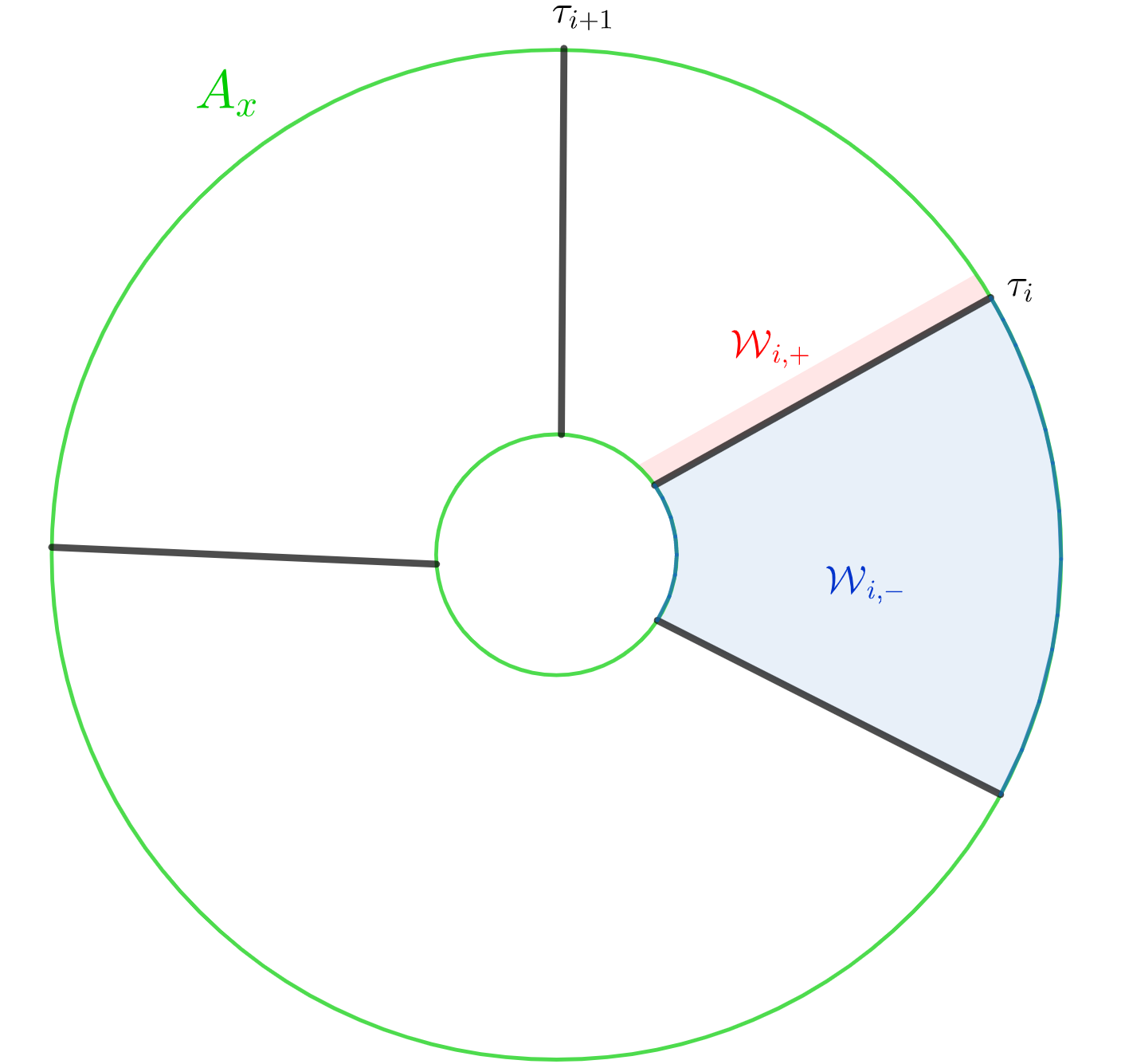
Figure 3.

As in the proof of Theorem 5.20, there is a gauge transformation $\varPsi_{i}:(\prescript{k}{}{\mathsf{PV}}^{*}_{\text{sf}}|_{\mathscr{W}_{i}},\bar{\partial}_{0})\rightarrow(\prescript{k}{}{\mathsf{PV}}^{*}_{\text{sf}}|_{\mathscr{W}_{i}},\bar{\partial}_{0}+[\phi_{\text{in}}+\phi_{\text{s}},\cdot])$ on each $\mathscr{W}_{i}$, where $\varPsi_{i}=e^{[\theta_{v,\rho},\cdot]}\circ e^{[\theta_{\tau},\cdot]}$ for a slab and $\varPsi_{i}=e^{[\theta_{\tau},\cdot]}$ for a wall. These are step function like elements in the gauge group satisfying

$$\varPsi_{i}=\begin{dcases}\Theta_{i}&\text{on $\mathscr{W}_{i,+}$,}\\ \text{id}&\text{on $\mathscr{W}_{i,-}$,},\end{dcases}$$

where $\Theta_{i}$ is the wall crossing factor associated to $\tau_{i}$. On the overlap $\mathscr{W}_{i,+}=\mathscr{W}_{i}\cap\mathscr{W}_{i+1}$ (if $i=s$, $i+1=1$), there is a commutative diagram

allowing us to understand the wall crossing factor $\Theta_{i}$ as the gluing between $(\prescript{k}{}{\mathsf{PV}}^{*}_{\text{sf}}|_{\mathscr{W}_{i}},\bar{\partial}_{0})$ and $(\prescript{k}{}{\mathsf{PV}}^{*}_{\text{sf}}|_{\mathscr{W}_{i+1}},\bar{\partial}_{0})$ over $\mathscr{W}_{i,+}$.

Notice that the Maurer-Cartan element $\phi$ is global. On a small neighborhood $W_{\alpha}$ containing $U_{x}\times D_{x}$, we have the sheaf $(\prescript{k}{}{PV}_{\alpha}^{*},\bar{\partial}_{\phi})$ on $W_{\alpha}$, and there is an isomorphism $e^{[\theta_{\alpha},\cdot]}:(\prescript{k}{}{PV}^{*}_{\alpha},\bar{\partial}_{\alpha})\cong(\prescript{k}{}{PV}^{*}_{\alpha},\bar{\partial}_{\phi}).$ Composing with the isomorphism $(\prescript{k}{}{PV}^{*}_{\alpha}|_{\mathscr{W}_{i}},\bar{\partial}_{\phi})\cong(\prescript{k}{}{\mathsf{PV}}^{*}_{\text{sf}}|_{\mathscr{W}_{i}},\bar{\partial}_{0}+[\phi_{\text{in}}+\phi_{\text{s}},\cdot])$, we have a commutative diagram of isomorphisms

$$\lx@xy@svg{\hbox{\raise 0.0pt\hbox{\kern 36.69643pt\hbox{\ignorespaces\ignorespaces\ignorespaces\hbox{\vtop{\kern 0.0pt\offinterlineskip\halign{\entry@#!@&&\entry@@#!@\cr&&\\&&\crcr}}}\ignorespaces{\hbox{\kern-36.69643pt\raise 0.0pt\hbox{\hbox{\kern 0.0pt\raise 0.0pt\hbox{\hbox{\kern 1.0pt\raise 0.0pt\hbox{$\textstyle{(\prescript{k}{}{\mathsf{PV}}^{*}_{\text{sf}}|_{\mathscr{W}_{i,+}},\bar{\partial}_{0})\ignorespaces\ignorespaces\ignorespaces\ignorespaces\ignorespaces\ignorespaces\ignorespaces\ignorespaces}$}}}}}}}\ignorespaces\ignorespaces\ignorespaces\ignorespaces{}{\hbox{\lx@xy@droprule}}\ignorespaces\ignorespaces\ignorespaces{\hbox{\kern 91.3762pt\raise 6.44008pt\hbox{{}\hbox{\kern 0.0pt\raise 0.0pt\hbox{\hbox{\kern 3.0pt\hbox{\hbox{\kern 0.0pt\raise-1.34326pt\hbox{$\scriptstyle{\varPsi_{i,0}}$}}}\kern 3.0pt}}}}}}\ignorespaces{\hbox{\kern 161.98961pt\raise 0.0pt\hbox{\hbox{\kern 0.0pt\raise 0.0pt\hbox{\lx@xy@tip{1}\lx@xy@tip{-1}}}}}}{\hbox{\lx@xy@droprule}}{\hbox{\lx@xy@droprule}}\ignorespaces\ignorespaces\ignorespaces{}\ignorespaces\ignorespaces{\hbox{\lx@xy@drawline@}}\ignorespaces{\hbox{\kern 71.30185pt\raise-28.59079pt\hbox{\hbox{\kern 0.0pt\raise 0.0pt\hbox{\lx@xy@tip{1}\lx@xy@tip{-1}}}}}}\ignorespaces\ignorespaces{\hbox{\lx@xy@drawline@}}\ignorespaces{\hbox{\lx@xy@drawline@}}{\hbox{\kern 98.34302pt\raise 0.0pt\hbox{\hbox{\kern 0.0pt\raise 0.0pt\hbox{\hbox{\kern 1.0pt\raise 0.0pt\hbox{$\textstyle{}$}}}}}}}{\hbox{\kern 161.98961pt\raise 0.0pt\hbox{\hbox{\kern 0.0pt\raise 0.0pt\hbox{\hbox{\kern 1.0pt\raise 0.0pt\hbox{$\textstyle{(\prescript{k}{}{\mathsf{PV}}^{*}_{\text{sf}}|_{\mathscr{W}_{i,+}},\bar{\partial}_{0})\ignorespaces\ignorespaces\ignorespaces\ignorespaces}$}}}}}}}\ignorespaces\ignorespaces\ignorespaces{}\ignorespaces\ignorespaces{\hbox{\lx@xy@drawline@}}\ignorespaces{\hbox{\kern 127.39517pt\raise-28.59079pt\hbox{\hbox{\kern 0.0pt\raise 0.0pt\hbox{\lx@xy@tip{1}\lx@xy@tip{-1}}}}}}\ignorespaces\ignorespaces{\hbox{\lx@xy@drawline@}}\ignorespaces{\hbox{\lx@xy@drawline@}}{\hbox{\kern-1.0pt\raise-39.83801pt\hbox{\hbox{\kern 0.0pt\raise 0.0pt\hbox{\hbox{\kern 1.0pt\raise 0.0pt\hbox{$\textstyle{}$}}}}}}}{\hbox{\kern 60.69643pt\raise-39.83801pt\hbox{\hbox{\kern 0.0pt\raise 0.0pt\hbox{\hbox{\kern 1.0pt\raise 0.0pt\hbox{$\textstyle{(\prescript{k}{}{PV}^{*}_{\alpha}|_{\mathscr{W}_{i,+}},\bar{\partial}_{\alpha})}$}}}}}}}{\hbox{\kern 197.68604pt\raise-39.83801pt\hbox{\hbox{\kern 0.0pt\raise 0.0pt\hbox{\hbox{\kern 1.0pt\raise 0.0pt\hbox{$\textstyle{}$}}}}}}}\ignorespaces}}}}\ignorespaces. \textstyle{(\prescript{k}{}{\mathsf{PV}}^{*}_{\text{sf}}|_{\mathscr{W}_{i,+}},\bar{\partial}_{0})\ignorespaces\ignorespaces\ignorespaces\ignorespaces\ignorespaces\ignorespaces\ignorespaces\ignorespaces} \scriptstyle{\varPsi_{i,0}} \textstyle{(\prescript{k}{}{\mathsf{PV}}^{*}_{\text{sf}}|_{\mathscr{W}_{i,+}},\bar{\partial}_{0})\ignorespaces\ignorespaces\ignorespaces\ignorespaces} \textstyle{(\prescript{k}{}{PV}^{*}_{\alpha}|_{\mathscr{W}_{i,+}},\bar{\partial}_{\alpha})} \textstyle{(\prescript{k}{}{\mathsf{PV}}^{*}_{\text{sf}}|_{\mathscr{W}_{i,+}},\bar{\partial}_{0})\ignorespaces\ignorespaces\ignorespaces\ignorespaces\ignorespaces\ignorespaces\ignorespaces\ignorespaces} \scriptstyle{\varPsi_{i,0}} \textstyle{(\prescript{k}{}{\mathsf{PV}}^{*}_{\text{sf}}|_{\mathscr{W}_{i,+}},\bar{\partial}_{0})\ignorespaces\ignorespaces\ignorespaces\ignorespaces} \textstyle{(\prescript{k}{}{PV}^{*}_{\alpha}|_{\mathscr{W}_{i,+}},\bar{\partial}_{\alpha})}$$

It is a Čech-type cocycle condition between the sheaves $\prescript{k}{}{\mathsf{PV}}^{*}_{\text{sf}}|_{\mathscr{W}_{i}}$’s and $\prescript{k}{}{PV}^{*}_{\alpha}$, which can be understood as the original consistency condition defined using path-ordered products in [24, 20]. In particular, taking a local holomorphic function in $\prescript{k}{}{\mathcal{G}}^{0}_{\alpha}(W_{\alpha})$ and restricting it to $U_{x}\times A_{x}$, we obtain elements in $\prescript{k}{}{\mathsf{G}}^{0}_{\text{sf}}(\mathscr{W}_{i})$ that jump across the walls according to the wall crossing factors $\Theta_{i}$’s.

Appendix A The Hartogs extension property

The following lemma is an application of the Hartogs extension theorem [29].

Lemma A.1.

Consider the analytic space $(\mathbb{C}^{*})^{k}\times\text{Spec}_{\text{an}}(\mathbb{C}[\Sigma_{\tau}])$ for some $\tau$ and an open subset of the form $U\times V$, where $U\subset(\mathbb{C}^{*})^{k}$ and $V$ is a neighborhood of the origin $o\in\text{Spec}_{\text{an}}(\mathbb{C}[\Sigma_{\tau}])$. Let $W:=V\setminus\big{(}\bigcup_{\omega}V_{\omega}\big{)}$, where $\dim(\omega)+2\leq\dim(\Sigma_{\tau})$ (i.e. $W$ is the complement of complex codimension $2$ orbits in $V$). Then the restriction $\mathcal{O}(U\times V)\rightarrow\mathcal{O}(U\times W)$ is a ring isomorphism.

Proof.

We first consider the case where $\dim(\Sigma_{\tau})\geq 2$ and $W=V\setminus\{0\}$. We can further assume that $\Sigma_{\tau}$ consists of just one cone $\sigma$, because the holomorphic functions on $V$ are those on $V\cap\sigma$ that agree on the overlaps. So we can write

$$\mathcal{O}(U\times W)=\left\{\sum_{m\in\Lambda_{\sigma}}a_{m}z^{m}\ |\ a_{m}\in\mathcal{O}_{(\mathbb{C}^{*})^{k}}(U)\right\},$$

i.e. as Laurent series converging in $W$. We may further assume that $W$ is a sufficiently small Stein open subset. Take $f=\sum_{m\in\Lambda_{\sigma}}a_{m}z^{m}\in\mathcal{O}(U\times W)$. We have the corresponding holomorphic function $\sum_{m\in\Lambda_{\sigma}}a_{m}(u)z^{m}$ on $W$ for each point $u\in U$, which can be extended to $V$ using the Hartogs extension theorem [29] because $\{0\}$ is a compact subset of $V$ such that $W$ is connected. Therefore, we have $a_{m}(u)=0$ for $m\notin\sigma\cap\Lambda_{\sigma}$ for each $u$, and hence $f=\sum_{\sigma\cap\Lambda_{\sigma}}a_{m}z^{m}$ is an element in $\mathcal{O}(U\times V)$.

For the general case, we use induction on the codimension of $\omega$ to show that any holomorphic function can be extended through $V_{\omega}\setminus\bigcup_{\tau}V_{\tau}$ with $\dim(\tau)<\dim(\omega)$. Taking a point $x\in V_{\omega}\setminus\bigcup_{\tau}V_{\tau}$, a neighborhood of $x$ can be written as $(\mathbb{C}^{*})^{l}\times\text{Spec}_{\text{an}}(\mathbb{C}[\Sigma_{\omega}])$, and by induction hypothesis, we know that holomorphic functions can already be extended through $(\mathbb{C}^{*})^{l}\times\{0\}$. We conclude that any holomorphic function can be extended through $V_{\omega}\setminus\bigcup_{\tau}V_{\tau}$. ∎

We will make use of the following version of the Hartogs extension theorem, which can be found in e.g. [21, p. 58], to handle extension within codimension $1$ cells $\rho$’s and maximal cells $\sigma$’s.

Theorem A.2 (Hartogs extension theorem, see e.g. [21]).

Let $U\subset\mathbb{C}^{n}$ be a domain with $n\geq 2$, and $A\subset U$ such that $U\setminus A$ is still a domain. Suppose $\pi(U)\setminus\pi(A)$ is a non-empty open subset, and $\pi^{-1}(\pi(x))\cap A$ is compact for every $x\in A$, where $\pi:\mathbb{C}^{n}\rightarrow\mathbb{C}^{n-1}$ is projection along one of the coordinate direction. Then the natural restriction $\mathcal{O}(U)\rightarrow\mathcal{O}(U\setminus A)$ is an isomorphism.

Proof of Lemma 5.15.

To prove the first statement, we apply Lemma A.1. So we only need to show that, for $\rho\in\mathscr{P}^{[n-1]}$, a holomorphic function $f$ in $U_{x}\setminus\mathscr{S}\subset V(\rho)$ can be extended uniquely to $U_{x}$, where $U_{x}$ is some neighborhood of $x\in\text{int}_{\text{re}}(\rho)\cap\mathscr{S}$. Writing $V(\rho)=(\mathbb{C}^{*})^{n-1}\times\text{Spec}_{\text{an}}(\mathbb{C}[\Sigma_{\rho}])$, we may simply prove that this is the case with $\Sigma_{\rho}$ consisting of a single ray $\sigma$ as in the proof of Lemma A.1. Thus we can assume that $V(\rho)=(\mathbb{C}^{*})^{n-1}\times\mathbb{C}$, and the open subset $U_{x}=U\times V$ for some connected $U$. We observe that extension of holomorphic functions from $(U\setminus\mathscr{S})\times V$ to $U\times V$ can be done by covering the former open subset with Hartogs’ figures.

To prove the second statement, we need to further consider extension through $\text{int}_{\text{re}}(\mathfrak{j})$ for a joint $\mathfrak{j}$. For those joints lying in some codimension $1$ stratum $\rho$, the argument is similar to the above. So we assume that $\sigma_{\mathfrak{j}}=\sigma$ is a maximal cell. We take a point $x\in\text{int}_{\text{re}}(\mathfrak{j})$ and work in a sufficiently small neighborhood $U$ of $x$. In this case, we may find a codimension $1$ rational hyperplane $\omega$ containing $\mathfrak{j}$, together with the lattice embedding $\Lambda_{\omega}\hookrightarrow\Lambda_{\sigma}$ inducing a projection $\pi:(\mathbb{C}^{*})^{n}\rightarrow(\mathbb{C}^{*})^{n-1}$ along one of the coordinate direction. Letting $A=\nu^{-1}(A\cap U)$ and applying Theorem A.2, we obtain the extensions for holomorphic functions in $U$. ∎

References

- [1] S. Barannikov, Generalized periods and mirror symmetry in dimensions , preprint, arXiv:math/9903124.
- [2] S. Barannikov and M. Kontsevich, Frobenius manifolds and formality of Lie algebras of polyvector fields, Internat. Math. Res. Notices (1998), no. 4, 201–215.
- [3] S. Bardwell-Evans, M.-W. Cheung, H. Hong, and Y.-S. Lin, Scattering diagrams from holomorphic discs in log Calabi-Yau surfaces, preprint, arXiv:2110.15234.
- [4] H. Cartan, Variétés analytiques réelles et variétés analytiques complexes, Bull. Soc. Math. France 85 (1957), no. 19.7, 77.
- [5] K. Chan, N. C. Leung, and Z. N. Ma, Geometry of the Maurer-Cartan equation near degenerate Calabi-Yau varieties, J. Differential Geom., to appear, arXiv:1902.11174.
- [6] by same author, Scattering diagrams from asymptotic analysis on Maurer-Cartan equations, J. Eur. Math. Soc. (JEMS) 24 (2022), no. 3, 773–849.
- [7] K. Chan and Z. N. Ma, Tropical counting from asymptotic analysis on Maurer-Cartan equations, Trans. Amer. Math. Soc. 373 (2020), no. 9, 6411–6450.
- [8] M.-W. Cheung and Y.-S. Lin, Some examples of family Floer mirror, preprint, arXiv:2101.07079.
- [9] C.-H. Cho, H. Hong, and S.-C. Lau, Gluing localized mirror functors, preprint, arXiv:1810.02045.
- [10] by same author, Localized mirror functor for Lagrangian immersions, and homological mirror symmetry for , J. Differential Geom. 106 (2017), no. 1, 45–126.
- [11] J.-P. Demailly, Complex analytic and differential geometry, 2012, https://www-fourier.ujf-grenoble.fr/ demailly/manuscripts/agbook.pdf.
- [12] J. L. Dupont, Simplicial de Rham cohomology and characteristic classes of flat bundles, Topology 15 (1976), no. 3, 233–245.
- [13] S. Felten, Log smooth deformation theory via Gerstenhaber algebras, Manuscripta Math. 167 (2022), no. 1-2, 1–35.
- [14] S. Felten, M. Filip, and H. Ruddat, Smoothing toroidal crossing spaces, Forum Math. Pi 9 (2021), Paper No. e7, 36.
- [15] A. Floer, Morse theory for Lagrangian intersections, J. Differential Geom. 28 (1988), no. 3, 513–547.
- [16] K. Fukaya, Multivalued Morse theory, asymptotic analysis and mirror symmetry, Graphs and patterns in mathematics and theoretical physics, Proc. Sympos. Pure Math., vol. 73, Amer. Math. Soc., Providence, RI, 2005, pp. 205–278.
- [17] K. Fukaya and Y.-G. Oh, Zero-loop open strings in the cotangent bundle and Morse homotopy, Asian J. Math. 1 (1997), no. 1, 96–180.
- [18] M. Gross and B. Siebert, Mirror symmetry via logarithmic degeneration data. I, J. Differential Geom. 72 (2006), no. 2, 169–338. MR 2213573 (2007b:14087)
- [19] by same author, Mirror symmetry via logarithmic degeneration data, II, J. Algebraic Geom. 19 (2010), no. 4, 679–780. MR 2669728 (2011m:14066)
- [20] by same author, From real affine geometry to complex geometry, Ann. of Math. (2) 174 (2011), no. 3, 1301–1428. MR 2846484
- [21] M. Jarnicki and P. Pflug, First steps in several complex variables: Reinhardt domains, EMS Textbooks in Mathematics, European Mathematical Society (EMS), Zürich, 2008.
- [22] L. Katzarkov, M. Kontsevich, and T. Pantev, Hodge theoretic aspects of mirror symmetry, From Hodge theory to integrability and TQFT tt*-geometry, Proc. Sympos. Pure Math., vol. 78, Amer. Math. Soc., Providence, RI, 2008, pp. 87–174.
- [23] Y. Kawamata and Y. Namikawa, Logarithmic deformations of normal crossing varieties and smoothing of degenerate Calabi-Yau varieties, Invent. Math. 118 (1994), no. 3, 395–409.
- [24] M. Kontsevich and Y. Soibelman, Affine structures and non-Archimedean analytic spaces, The unity of mathematics, Progr. Math., vol. 244, Birkhäuser Boston, Boston, MA, 2006, pp. 321–385.
- [25] N. C. Leung, Z. N. Ma, and M. B. Young, Refined scattering diagrams and theta functions from asymptotic analysis of Maurer-Cartan equations, Int. Math. Res. Not. IMRN (2021), no. 5, 3389–3437.
- [26] Y.-S. Lin, Correspondence theorem between holomorphic discs and tropical discs on K3 surfaces, J. Differential Geom. 117 (2021), no. 1, 41–92.
- [27] G. Mikhalkin, Enumerative tropical algebraic geometry in , J. Amer. Math. Soc. 18 (2005), no. 2, 313–377. MR 2137980 (2006b:14097)
- [28] T. Nishinou and B. Siebert, Toric degenerations of toric varieties and tropical curves, Duke Math. J. 135 (2006), no. 1, 1–51. MR 2259922 (2007h:14083)
- [29] H. Rossi, Vector fields on analytic spaces, Ann. of Math. (2) 78 (1963), 455–467.
- [30] H. Ruddat, Log Hodge groups on a toric Calabi-Yau degeneration, Mirror symmetry and tropical geometry, Contemp. Math., vol. 527, Amer. Math. Soc., Providence, RI, 2010, pp. 113–164.
- [31] H. Ruddat and B. Siebert, Period integrals from wall structures via tropical cycles, canonical coordinates in mirror symmetry and analyticity of toric degenerations, Publ. Math. Inst. Hautes Études Sci. 132 (2020), 1–82.
- [32] H. Ruddat and I. Zharkov, Topological Strominger-Yau-Zaslow fibrations, in preparation.
- [33] by same author, Compactifying torus fibrations over integral affine manifolds with singularities, 2019–20 MATRIX annals, MATRIX Book Ser., vol. 4, Springer, Cham, [2021] ©2021, pp. 609–622.
- [34] A. Strominger, S.-T. Yau, and E. Zaslow, Mirror symmetry is -duality, Nuclear Phys. B 479 (1996), no. 1-2, 243–259.
- [35] J. Terilla, Smoothness theorem for differential BV algebras, J. Topol. 1 (2008), no. 3, 693–702.
- [36] H. Whitney, Geometric integration theory, Princeton University Press, Princeton, N. J., 1957.