1 Introduction

There has been a growing interest in applications involving the causal-noncausal Vector Autoregressive (VAR) models and in their theoretical properties [Hecq, Lieb, Telg (2016), Davis, Song (2020), Lanne, Luoto (2021), Swensen (2022)]. Most of the currently available inference methods for these processes are either simulation-based, or Bayesian, or arise as extensions of maximum-likelihood-based methods for causal VAR models. Especially, only simulation-based and Bayesian methods of forecasting from mixed causal-noncausal VAR processes are currently available, and in the early literature their causal predictive densities were believed to be without tractable closed-form expressions [see Lanne, Luoto, Saikkonen (2012), Nyberg, Saikkonen (2014)].

This paper provides an alternative forecasting method for multivariate processes based on a closed-form expression of the predictive density. It builds upon the results on predictive densities of noncausal processes given in Gourieroux, Jasiak (2016) and introduces a new closed-form expression of predictive density for multivariate causal-noncausal VAR processes at horizon 1. The predictive densities at any horizon higher than 1 are obtained by applying a Sampling Importance Resampling (SIR) procedure. The proposed forecasting method is applicable to Structural (SVAR) models, which are the mixed causal-noncausal VAR models satisfying an assumption of cross-sectionally independent errors.

In this class of processes, the error independence condition helps identify the autoregressive parameters and suggests a suitable error orthogonalization method. We show that in the (S)VAR model, it is possible to implement an impulse response analysis, which is consistent with the classical definition of an impulse response function tracing out ”the consequences of an increase in the jth variable’s innovation at date $t$ for the value of the ith variable at time $t+s$, holding all other variables dated $t$ or earlier constant” [Hamilton (1994)]. The proposed impulse response functions are computed from nonlinear causal innovations, which are introduced for mixed causal-noncausal processes as well, by extending the results in Koop, Pesaran, Potter (1996), Gourieroux, Jasiak (2005) and are in line with those in Gonzalves et al.(2022). We define the nonlinear causal innovations for a mixed causal-noncausal (S)VAR model and determine their relationship with the errors of the (S)VAR model. The effects of shocks applied separately to nonlinear causal innovations associated with the causal and non-causal components of a multivariate process $Y_{t}$ are discussed and the impulse response functions (IRF) and their term structure are described.

The forecast performance and the impulse response analysis are illustrated by simulated and estimated time series. We use semi-parametric estimators introduced in Gourieroux, Jasiak (2017), (2022) to estimate the (S)VAR models, and compute their residuals and nonlinear causal innovations. This approach does not require distributional assumptions on the errors of a (S)VAR model and is in line with the recent literature on SVAR models [Guay (2021)]. The semi-parametric estimation distinguishes our approach from the existing literature employing maximum likelihood-based methods [Davis, Song (2020), Swensen (2022)] .

The paper is organized as follows. Section 2 describes the (Structural) causal-noncausal VAR model. Section 3 presents the closed-form formula of multivariate predictive density. Section 4 describes the nonlinear causal innovations and the derivation of impulse response functions. Section 5 presents the semi-parametric estimation of the mixed SVAR model. Section 6 provides an illustration based on a bivariate causal-noncausal model: A simulated mixed VAR process is examined, as well as a bivariate process of Bitcoin/USD and Ethereum/USD exchange rates. In addition, Section 6 discusses the uncertainty in the term structure of impulse response functions. Section 7 concludes. The technical results are given in Appendices 1-3. Appendix 1 contains the proof of the expression of the predictive density. Appendix 2 explains why some multivariate causal-noncausal VAR models proposed in the existing literature are incompatible with the Structural VAR (SVAR) representation. Appendix 3 discusses the (under)-identification of nonlinear innovations in a multivariate framework.

Additional information is provided in the online Appendices B and C, which include a discussion of the identification conditions for Independent Component Analysis (ICA) and the closed-form expression of the kernel-based semi-nonparametric estimator of predictive density, respectively.

2 The Mixed Causal-Noncausal (S)VAR(1) Model

Let us consider a strictly stationary solution $(Y_{t})$ of a Structural VAR model:

$$Y_{t} = \Phi_{1}Y_{t-1}+\cdots+\Phi_{p}Y_{t-p}+\varepsilon_{t},$$ (2.1)

$$= \Phi_{1}Y_{t-1}+\cdots+\Phi_{p}Y_{t-p}+Pu_{t},$$ (2.2)

where $Y_{t}$ is a vector of length $m$, $\Phi_{j},\,j=1,...,p$ are matrices of autoregressive coefficients of dimension $m\times m$, $P$ is an invertible $(m\times m)$ matrix and $(\varepsilon_{t})$ is a sequence of independent, identically distributed (i.i.d.) random vectors of dimension $m$ with mean zero and finite variance-covariance matrix $\Sigma$. The components $(u_{1t}),(u_{2t})...,(u_{mt})$ are i.i.d. and are cross-sectionally independent of one another. The cross-sectional independence condition is necessary to discuss the impulse response functions in a nonlinear framework. The stationarity assumption implies that the determinant of the autoregressive polynomial has no roots on the unit circle.

2.1 Identification Issues

The classical methods of estimation and testing for SVAR models are based on the first and second-order moments, such as the means, variances and autocovariances/autocorrelations, which is equivalent to assuming Gaussian error distributions. Under the assumption of Gaussian errors $\varepsilon_{t}$, two identification issues arise:

i) Matrix $P$ is not identifiable

If $u_{t},\,t=1,...,T$ are standard normal variables, $u_{t}\sim N(0,Id)$, where $Id$ denotes the identity matrix and matrix $P$ is an orthogonal matrix $PP^{\prime}=Id$, then the distribution of $\varepsilon_{t}$ is also standard normal.

ii) The roots of the autoregressive polynomial cannot be distinguished from their reciprocals.

The autoregressive matrix coefficients $\Phi_{1},...,\Phi_{p}$ can be computed from the Yule-Walker equations for multivariate autocovariances. The system of Yule-Walker equations yields several solutions in $\Phi_{1},...,\Phi_{p}$, which can be distinguished by considering the values of the roots of the characteristic equation $\det(Id-\Phi_{1}z+\cdots+\Phi_{p}z^{p})=0$. Let the set of roots be denoted by $\lambda_{j},\;j=1,...,mp$. The Yule-Walker equations are satisfied by either the autoregressive coefficient matrices associated with roots $\lambda_{j},\;j=1,...,mp$, or $1/\lambda_{j},\;j=1,...,mp$. Thus, in general the Yule-Walker equations have $2^{mp}$ solutions in $\Phi_{1},...,\Phi_{p}$, if the roots are distinct [see Velasco (2022), Section 2].

The first identification issue is usually solved by introducing identifying restrictions, such as the causal ordering, i.e. the Cholesky decomposition [Sims (1980), (2002)], which has been criticized by e.g. Lutkepohl (1990), or by imposing additional restrictions such as the equality restrictions [Rubio-Ramirez, Waggoner , Zha (2010)], sign restrictions [Grangiera, Moon, Schorfheide (2018)], or long-run restrictions [see Blanchard, Quah (1989), Cochrane (1994), Section 2.1.5, Faust, Leeper (1997), Leeper et al. (2013)].

The second identification issue has been addressed recently in the literature on noncausal multivariate models. Nevertheless, the standard least squares procedures implemented in commonly used software for multivariate time series analysis are set to always provide autoregressive coefficients estimators such that the roots of the estimated autoregressive polynomial are located outside the unit circle. In many instances, this least squares estimation method leads to misleading results [see the discussion in Lanne, Saikkonen (2011)].

2.2 Independent Non-Gaussian Errors

It follows from the Independent Component Analysis (ICA) literature [Comon (1994), Erikson, Koivunen (2004)] and the existence of two-sided moving average representation [Chan, Ho, Tong (2006)] that the two identification issues i) and ii) can be solved without imposing identifying restrictions if the components $u_{j,t}$ of the error vector $u_{t}$ are independent of one another and non-Gaussian [Gourieroux, Monfort, Renne (2017), Lobato, Velasco (2018), Velasco (2022)]. In some sense, the Gaussian distribution is not representative of the set of error distributions. In such a case, it is possible to identify the autoregressive coefficient matrices $\Phi_{1},...,\Phi_{p}$, matrix $P$ and also to identify non-parametrically the distributions of variables $u_{j,t},j=1,...,m$. The error independence conditions determine the structural characteristic of the VAR model.

The exact conditions on the distributions of $u_{t}$ components allowing us to solve the identification issues are reviewed in the on-line Appendix B.

2.3 Mixed Causal-Noncausal Processes

When the roots of the autoregressive polynomial matrix are either outside, or inside the unit circle, there exists a unique stationary solution to the VAR system (1.1)-(1.2). This stationary solution can be written as a two-sided moving average in errors $\varepsilon_{t}$:

$$Y_{t}=\sum_{j=-\infty}^{+\infty}C_{j}\varepsilon_{t-j}.$$ (2.3)

This is a linear time series, according to the terminology used in Rosenblatt (2012). It is said to be causal in $\varepsilon_{t}$, if $Y_{t}=\sum_{j=0}^{+\infty}C_{j}\varepsilon_{t-j}$, or noncausal in $\varepsilon_{t}$, if $Y_{t}=\sum_{j=-\infty}^{-1}C_{j}\varepsilon_{t-j}=\sum_{j=1}^{+\infty}C_{-j}\varepsilon_{t+j}$, or mixed causal-noncausal, otherwise.

In either case, process $(Y_{t})$ can be characterized by a possibly complex conditional distribution of $Y_{t+h}$ given $\underline{Y_{t}}=(Y_{t},Y_{t-1},...)$ for $h=1,2,..$, that provides nonlinear predictions and impulse response functions. In the presence of a noncausal, or mixed causal-noncausal representation, process $(Y_{t})$ has nonlinear dynamics and may display local trends and bubbles [Gourieroux, Zakoian (2017), Gourieroux, Jasiak (2017)].

3 Predictive Density

Let us consider a VAR(p) process of dimension $m$:

$$Y_{t}=\Phi_{1}Y_{t-1}+\cdots+\Phi_{p}Y_{t-p}+\varepsilon_{t},$$ (3.1)

where the error vectors $\varepsilon_{t}$ are i.i.d. and have a continuous distribution with probability density function $g$. We also assume that the roots of:

$$\det(Id-\Phi_{1}z-\cdots-\Phi_{p}z^{p})=0,$$ (3.2)

are not on the unit circle. Then, there exists a unique stationary solution of model (3.1) with a two-sided moving average representation in $\varepsilon_{t}$.

Remark 1: Alternatively, the model could have been written in a multiplicative representation proposed by Lanne, Saikkonen (2008),(2013) as:

$$\Phi(L)\Psi(L^{-1})Y_{t}=\epsilon_{t}^{*},$$

where matrix autoregressive polynomials $\Phi$ and $\Psi$ have both roots outside the unit circle and $\epsilon_{t}^{*}$ is an i.i.d. sequence of vectors. Appendix 2 shows that this latter representation may not be compatible with the SVAR model (2.1).

By stacking the present and lagged values of process $(Y_{t})$, model (3.1) can be rewritten as a $n=mp$ multidimensional VAR(1) model:

$$\left(\begin{array}[]{c}Y_{t}\\ \tilde{Y}_{t-1}\end{array}\right)=\left(\begin{array}[]{c}Y_{t}\\ Y_{t-1}\\ \vdots\\ Y_{t-p+1}\end{array}\right)=\Psi\left(\begin{array}[]{c}Y_{t-1}\\ \tilde{Y}_{t-2}\end{array}\right)+\left(\begin{array}[]{c}\varepsilon_{t}\\ 0\end{array}\right),$$ (3.3)

with

$$\Psi=\left(\begin{array}[]{cccc}\Phi_{1}&\cdots&\cdots&\Phi_{p}\\ Id&0&\cdots&\\ \vdots&\ddots&\ddots&\vdots\\ 0&\cdots&Id&0\end{array}\right).$$ (3.4)

The eigenvalues of the autoregressive matrix $\Psi$ are the reciprocals of the roots of the characteristic equation (3.2).

Matrix $\Psi$ has a Jordan representation:

$$\Psi=A\left(\begin{array}[]{cc}J_{1}&0\\ 0&J_{2}\end{array}\right)A^{-1},$$

where $J_{1}$ (resp. $J_{2}$) are real $(n_{1}\times n_{1})$ (resp. $(n_{2}\times n_{2})$) matrices where $n_{2}=n-n_{1}$ with all eigenvalues of modulus strictly less than 1 [resp. strictly larger than 1] and $A$ is a ($n\times n$) invertible matrix [see Perko (2001), Gourieroux, Jasiak (2016), Section 5.2, Davis, Song (2020), Remark 2.1. for real Jordan representations]. Then, equation (3.4) can be rewritten as:

$$A^{-1}\left(\begin{array}[]{c}Y_{t}\\ \tilde{Y}_{t-1}\end{array}\right)=\left(\begin{array}[]{cc}J_{1}&0\\ 0&J_{2}\end{array}\right)A^{-1}\left(\begin{array}[]{c}Y_{t-1}\\ \tilde{Y}_{t-2}\end{array}\right)+A^{-1}\left(\begin{array}[]{c}\varepsilon_{t}\\ 0\end{array}\right).$$ (3.5)

Let us introduce a block decomposition of $A^{-1}$:

$$A^{-1}=\left(\begin{array}[]{c}A^{1}\\ A^{2}\end{array}\right),$$ (3.6)

where $A^{1}$ is of dimension $(n_{1},n)$ and the transformed variables:

$$Z_{t}=\left(\begin{array}[]{c}Z_{1,t}\\ Z_{2,t}\end{array}\right)=A^{-1}\left(\begin{array}[]{c}Y_{t}\\ \tilde{Y}_{t-1}\end{array}\right),\;\;\;\eta_{t}=\left(\begin{array}[]{c}\eta_{1,t}\\ \eta_{2,t}\end{array}\right)=A^{-1}\left(\begin{array}[]{c}\varepsilon_{t}\\ 0\end{array}\right).$$ (3.7)

Then, we get:

$$Z_{1,t} = J_{1}Z_{1,t-1}+\eta_{1,t},$$

$$Z_{2,t} = J_{2}Z_{2,t-1}+\eta_{2,t}.$$ (3.8)

The first set of equations in system (3.8) defines a causal VAR(1) model. Thus, process $Z_{1}$ has the causal MA$(\infty)$ representation:

$$Z_{1,t}=\sum_{j=0}^{+\infty}J_{1}\eta_{1,t-j},$$ (3.9)

with $\eta_{1,t}$ as the causal innovation of $Z_{1,t}$.

The second set of equations in system (3.8) needs to be inverted to obtain a MA representation in matrices with eigenvalues of modulus strictly less than 1. We get:

$$Z_{2,t} = J_{2}^{-1}Z_{2,t+1}-J_{2}^{-1}\,\eta_{2,t+1},$$ (3.10)

$$= -\sum_{j=0}^{+\infty}[J_{2}^{-j-1}\,\eta_{2,t+j+1}].$$

Therefore, $(Z_{2,t})$ is a noncausal process with a one-sided moving average representation in future values $\varepsilon_{t+1},\varepsilon_{t+2},...,$. While this noncausal component is a linear function of future values of $\eta_{2,t}$, it has nonlinear dynamics in the calendar time.

The expression of the predictive density of $Y_{T+1}$ given $\underline{Y}_{T}=(Y_{T},Y_{T-1},...)$ is given below and derived in Appendix 1.

Proposition 1: The conditional probability density function (pdf) of $Y_{T+1}$ given $\underline{Y}_{T}$ is:

$$l(y|\underline{Y}_{T})=\frac{l_{2}\left[A^{2}\left(\begin{array}[]{c}y\\ \tilde{Y}_{T-1}\end{array}\right)\right]}{l_{2}\left[A^{2}\left(\begin{array}[]{c}Y_{T}\\ \tilde{Y}_{T-1}\end{array}\right)\right]}\,|\det J_{2}|\,g(y-\Phi_{1}Y_{T}-\cdots-\Phi_{p}Y_{T-p+1}),$$ (3.11)

where $l_{2}(z_{2})$ is the stationary pdf of $Z_{2,t}=A^{2}\left(\begin{array}[]{c}Y_{t}\\ \tilde{Y}_{t-1}\end{array}\right)$, if $n_{2}\geq 1$. In the pure noncausal process, $n_{2}=0$, we have:

$$l(y|\underline{Y}_{T})=g(y-\Phi_{1}Y_{T}-\cdots-\Phi_{p}Y_{T-p+1}).$$

Corollary 1: The mixed causal-noncausal process is a Markov process of order $p$ in the calendar time for $n_{2}\geq 1$.

This corollary extends to linear mixed causal-noncausal processes of any autoregressive order, the result of Cambanis, Fakhre-Zakeri (1994), who show that a linear pure noncausal autoregressive process of order 1 is a Markov process of order 1 in calendar time.

Remark 2: In the special case $p=1$ the predictive density becomes:

$$l(y|\underline{Y}_{T})=l(y|Y_{T})=\frac{l_{2}(A^{2}y)}{l_{1}(A^{2}Y_{T})}\,|\det J_{2}|\,g(y-\Phi Y_{T}).$$ (3.12)

There exists a multiplicity of Jordan representations and associated matrices $A$ built from ”extended” eigenspaces. However, $\det J_{2}=\prod_{j=1}^{n_{2}}\lambda_{j}$, where $|\lambda_{j}|>1,\,j=1,...,n_{2}$ is independent of the Jordan representation. Similarly, the noncausal component $Z_{2}$ is defined up to a linear invertible transformation. Since the Jacobian is the same for the numerator and denominator of the ratio $\frac{l_{2}\left[A^{2}\left(\begin{array}[]{c}y\\ \tilde{Y}_{T-1}\end{array}\right)\right]}{l_{2}\left[A^{2}\left(\begin{array}[]{c}Y_{T}\\ \tilde{Y}_{T-1}\end{array}\right)\right]}$, it has no effect on the ratio. Thus, the expression of $l(y|\underline{Y}_{T})$ does not depend on the selected Jordan representation.

In the VAR(1) model, we have $dim\,Z_{t}=dim\,Y_{t}$ and $Y_{t}=AZ_{t}$. Therefore, each component of $Y_{t}$ is a linear combination of the causal and noncausal components $Z_{1,t},Z_{2,t}$, respectively. When $p=2$, there exist more underlying causal and non-causal components.

A mixed VAR process has nonlinear causal dynamics, which is captured by the predictive density. In this non-linear, non-Gaussian framework, the predictive density provides prediction intervals at various horizons, replacing the linear pointwise predictions and prediction intervals.

The closed-form expression of the predictive density at horizon 1 allows us to perform drawings from that density by applying a Sampling Importance Resampling (SIR) method [Smith, Gelfand (1992), Tanner (1993)]. Predictions at horizons $h>1$ can be obtained as follows. By replicating $s=1,...,S$ times $h$ consecutive drawings of $Y_{T+1},...,Y_{t+h}$ we build the predictive distribution at horizon $h$. This procedure provides the SIR-based predictive density at any horizon $h$.

4 Nonlinear Innovations and Impulse Responses

In macroeconomics and finance, the inference on a (nonlinear) dynamic model commonly includes the computation of impulse response functions, which are a useful tool for economic and financial policy evaluation. That computation need to be consistent with the structural interpretation of the model. More specifically, the ”structural” IRFs have to be based on ”structural” shocks that need to be identified. These shocks have to satisfy serial and cross-sectional independence conditions and be past-dependent only [Gourieroux, Jasiak (2005), Gourieroux, Monfort, Renne (2017), Gonzalves, Herrera, Kilian, Pesavento (2022)]. We discuss below the identification of shocks in the framework of mixed SVAR models.

4.1 Nonlinear Innovations

Several types of errors can be defined from the mixed causal-noncausal models, such as the errors $(\varepsilon_{t})$, the causal errors $(\eta_{1,t})$ and the noncausal errors $(\eta_{2,t})$. Among them, only $(\eta_{1,t})$ can be interpreted as causal innovations, i.e. the causal innovations of $Z_{1,t}=A^{1}Y_{t}$.

The remaining errors $(\eta_{2,t})$ and components of $(\varepsilon_{t})$ do not have a causal interpretation. Therefore, they cannot be used directly to define and examine the impulse response functions [see Davis, Song (2020), Figure 1.7, for an approach different from the classical definition of IRF in noncausal models]. Therefore, nonlinear causal innovations need to be derived for any noncausal or mixed causal-noncausal VAR model.

Definition 1: A nonlinear causal innovation is a process $(v_{t})$ of dimension $m$ such that:

i) the variables $v_{t}$ are i.i.d. over time.

ii) the process $(Y_{t})$ can be written in a nonlinear autoregressive form:

$$Y_{t}=a(\tilde{Y}_{t-1},v_{t}).$$ (4.1)

It is easy to see that this condition is equivalent to the Markov of order $p$ property of $(Y_{t})$ with a continuous distribution and can be applied to the mixed model (3.1) by Corollary 1. The nonlinear causal innovations follow from the Volterra representation of a multivariate strictly stationary process, providing the basis of nonlinear impulse response functions [Potter (2000), Gourieroux, Jasiak (2005)]. When function $a$ is invertible with respect to $v$, we find that $v_{t}$ is a nonlinear function of $Y_{t}$ given its past. In the next section, $v_{t}$ is used to define the structural shocks. These shocks are nonlinear combinations of different variables, and are not associated with some specific observed variable [see e.g Cochrane (1994) p. 361 for a similar remark in a linear dynamic framework].

4.2 Impulse Response Functions (IRF)

The effect of simultaneous shocks in vector $\delta$ of length $m$ to $v_{T}$ at time $T$ on the distributions of future values $Y_{T+h},\;h=0,1,...,H$ can be examined from the nonlinear autoregressive model (4.1).

Let $\hat{v}_{T+h}^{s},\,h=0,...,H$ denote a joint path of future innovations drawn in the distribution of $v_{t}$. The simulated path prior to the shock, i.e. the baseline path $Y_{T+h}^{s},\,h=1,...,H$, can be found from recursions:

$$Y_{T+h}^{s}=a(\tilde{Y}_{T+h-1}^{s},v_{T+h}^{s}),\;\;h=0,...,H.$$

The shocked path $Y_{T+h}^{s}(\delta)$ is obtained by applying the propagation mechanism:

$$Y_{T}^{s}(\delta)=a(\tilde{Y}_{T-1}^{s},v_{T}^{s}+\delta),\;\;\mbox{for}\;h=0,$$

and $Y_{T+h}^{s}(\delta)=a(\tilde{Y}_{T+h-1}^{s}(\delta),v_{T+h}^{s}),\;$ for h=1,2,… . The difference $Y^{s}_{T+h}(\delta)-Y^{s}_{T+h},\,h=1,2,...,H$ is a function of $\delta$ and provides the term structure of IRF corresponding to scenario $s$.

By replicating this computation for $S$ simulations (scenarios), we get for a large $S$ and any $h$ the joint conditional distribution of $[Y_{T+h},Y_{T+h}(\delta)]$ given $\underline{Y}_{T}$ and the information on uncertainty about the IRF term structures. In particular, we can compare the conditional means $E[Y_{T+h}|\underline{Y}_{T}]$ and $E[Y_{T+h}(\delta)|\underline{Y}_{T}]$, the conditional variances $V[Y_{T+h}(\delta)-Y_{T+h}|\underline{Y}_{T}]$ and the conditional prediction intervals [Koop, Pesaran, Potter (1996), Gourieroux, Jasiak (2005)]. The conditional correlation $Corr[(Y_{T+h},Y_{T+h}(\delta)|\underline{Y}_{T}]$ is also informative, especially for mixed models, as it allows us to trace out the effects of shocks along the speculative bubbles.

4.3 The Identification of Causal Shocks

The nonlinear innovations are not defined in a unique way, even under an additional condition of independence of components $(v_{1,t}),...,(v_{m,t})$, which is required to appropriately define the notion of a shock to one innovation $v_{2,t}$, say, with no effect on the remaining components of $v_{t}$. This identification issue is examined in Appendix 3 in a functional framework. In particular, we get the following Proposition:

Proposition 2:

In a VAR(1) process, the dimension of under-identification in the functional space of nonlinear innovations is finite and equal to $2m$.

Therefore, the identification of structural shocks is an issue in the mixed causal-noncausal VAR models, similarly to the linear causal Gaussian VAR models.

Nevertheless, the aplications of mixed causal-noncausal models indicate that the noncausal order is often equal to 1, i.e. $n_{2}=1$ [see e.g. Gourieroux, Jasiak (2017), Hecq, Lieb, Telg (2016), and Section 6.3 of this paper]. This is likely due to the type of nonlinear dynamics generated by noncausal roots capturing the speculative bubbles and local trends. For example, in macroeconomic models, the noncausal effect is mainly due to speculative bubbles in gas prices impacting jointly the consumer price index (CPI), GDP and unemployment rate. For this reason, some papers on causal VAR models for macroeconomic data include an index of sensitive commodity prices [Christiano, Eichenbaum, Evans (1996)].

It is interesting to examine if one can shock the noncausal component $(Z_{2})$, which determines the nonlinear dynamics of the model, independently of the causal component $(Z_{1})$. Let us consider a VAR(1) model with $n_{2}=1$. We can define, up to an increasing transformation, the nonlinear innovation associated with $Z_{2,t}=A^{2}Y_{t}$ as:

$$v_{2,t}=F_{2}[Z_{2,t}|\underline{Y}_{t-1}],$$ (4.2)

which is the conditional cumulated distribution function (c.d.f) of $Z_{2,t}$. Next we can append it by vector $\eta_{1,t}=A^{1}\varepsilon_{t}$ of dimension $n-1$ to obtain a complete vector of causal innovations $v_{t}=(\eta_{1,t}^{\prime},v_{2,t})^{\prime}$. Obviously, there is a priori no reason for $v_{1,t}=\eta_{1,t}$ to be independent of $v_{2,t}$, which is a necessary condition to perform the IRF of a (structural) shock to $v_{2,t}$ without an effect on $\eta_{1,t}$. Therefore, before deriving the effect of a shock on the ”noncausal” component, we need to check if the independence condition holds. The test of independence hypothesis can be applied to the residuals $\hat{v}_{1,t}=\hat{\eta}_{1,t},\hat{v}_{2,t}$. A following alternative approach can also be used to check if the independence condition is satisfied. Let us consider the SVAR model (2.1):

$$Y_{t}=\Phi Y_{t-1}+\varepsilon_{t}=\Phi Y_{t-1}+Pu_{t},$$ (4.3)

where the components $(u_{1,t}),...,(u_{m,t})$ are independent and defined up to permutation and scale effects. These independent errors are identifiable. Hence, we can check if one of the error processes $u_{k,t}$, say, satisfies a one-to-one (nonlinear) relationship with $(v_{2,t})$ and the other errors satisfy one-to-one relationships with $(\eta_{1,t})$. The idea is to project nonlinearly the residual $\hat{v}_{2,t}$ on the estimated errors $\hat{u}_{t}$.

As an example, let us consider a macroeconomic VAR model including oil prices. If $n_{2}=1$ and $v_{2}$ is identifiable (up to a nonlinear increasing function), and if the dynamics of $Z_{2}$ resemble the oil prices, then the shock to $v_{2}$ is seen as a shock to oil prices.

The nonlinear dynamics generated by the noncausal component can sometimes help identify the ”noncausal” shock. Otherwise, there is an identification issue and the structural shocks to $v$ have to be considered jointly, as the simultaneity cannot be eliminated.

5 Semi-Parametric Estimation

The mixed SVAR model can be estimated by the maximum likelihood method based on an assumed parametric distribution of $\varepsilon_{t}$, or $u_{t}$ [see Breidt et al. (1991), Lanne, Saikkonen (2010), (2013), Davis, Song (2020), Bec et al (2020)]. This approach yields consistent estimators provided that the distributional assumption is valid.

Alternatively, the mixed (S)VAR model can be consistently estimated without any parametric assumptions on the error distribution by using either the (Generalized) Covariance (GCov) estimator [Gourieroux, Jasiak (2017), (2021) for the GCov estimator and Gourieroux, Monfort, Renne (2017), (2020)], moment estimators [see, Guay (2021), Lanne, Luoto (2021)], or minimum distance estimators based on cumulant spectral density of order 3 and 4 [Velasco, Lobato (2019), Velasco (2022)].

The GCov estimator provides asymptotically normally distributed and semi-parametrically efficient estimators . The estimation approach can be applied along the following lines:

step 1. Apply the GCov estimator to model (2.1) to obtain the estimators of matrices of autoregressive coefficients $\hat{\Phi}_{1},...,\hat{\Phi}_{p}$.

step 2. Use the $\hat{\Phi}_{i},i=1,...,p$ estimators to compute the roots of the lag-polynomial and more generally an estimated Jordan representation: $\hat{A},\hat{J}_{1},\hat{J}_{2}$.

step 3. Compute the error approximations using the estimates obtained in Step 1:$\hat{\varepsilon}_{t}=Y_{t}-\hat{\Phi}_{1}Y_{t-1}-...-\hat{\Phi}_{p}Y_{t-p}$.

step 4. Compute $\hat{Z}_{t}=\hat{A}^{-1}\left(\begin{array}[]{c}Y_{t}\\ \tilde{Y}_{t-1}\end{array}\right),\;\;\;\hat{\eta}_{t}=\hat{A}^{-1}\left(\begin{array}[]{c}\hat{\varepsilon}_{t}\\ 0\end{array}\right)$.

step 5. If the GCov or the pseudo-maximum likelihood estimator are applied to estimate the SVAR model (2.2), an Independent Component Analysis (ICA) analysis can be applied to the errors $\hat{\varepsilon}_{t}$, to provide a consistent estimator $\hat{P}$ of matrix $P$ and the approximations $\hat{u}_{t}$ of errors $u_{t}$.

step 6. The following densities can be estimated by kernel estimators applied to the approximated series:

- the density $g$ of $\varepsilon_{t}$ can be estimated from $\hat{\varepsilon}_{t},\;t=1,...,T$;

- the density $l_{2}$ of $Z_{2,t}$ can be estimated from $\hat{Z}_{2,t},\;t=1,...,T$;

- the densities of errors $u_{j,t},\,j=1,...,m$ can be estimated from $\hat{u}_{j,t},\,j=1,...,m,\;t=1,...,T$;

step 7. The predictive density can be estimated by replacing in the formula of Proposition 2 $l_{2}$ by $\hat{l}_{2}$, $A^{2}$ by $\hat{A}^{2}$, and also $J_{2}$ by $\hat{J}_{2}$, $g$ by $\hat{g}$, and $\Phi_{1},...,\Phi_{p}$ by $\hat{\Phi}_{1},...,\hat{\Phi}_{p}$. The mode of the predictive density provides the point forecasts and the quantiles of the predictive density can be used to obtain prediction intervals at horizon 1.

step 8. The nonlinear innovations $\hat{v}_{2,t}$ can be computed from the estimated distributions as $\hat{v}_{2,t}=\hat{F}_{2,T}(\hat{Z}_{2,t}|\underline{Y}_{t-1})$.

step 9. The independence between $v_{2,t}$ and $\eta_{1,t}$ can be tested.

step 10. The impulse response functions can be traced out and their term structures can be calculated.

6 Illustration

We illustrate the nonlinear forecasts and IRF in the causal-noncausal (S)VAR model. In the first part of this Section, we perform and discuss a Monte Carlo study. Next, we examine a forecast and IRF in an application to a bivariate series of Bitcoin/USD and Ethereum/USD exchange rates.

6.1 Simulation Study

6.1.1 The Data Generating Process

We consider a simulated trajectory of length 600 of a bivariate causal-noncausal VAR(1) process with the following matrix of autoregressive coefficients:

$$\Phi=\left(\begin{array}[]{cc}0.7&-1.3\\ 0&2\end{array}\right),$$

with eigenvalues 0.7 and 2, located inside and outside the unit circle, respectively. The errors follow a bivariate noise with independent components both t-student distributed with $\nu$ =4 degrees of freedom, mean zero and variance equal to $\nu/(\nu-2)=2$.

Matrix A is as follows:

$$A=\left(\begin{array}[]{cc}1&-1\\ 0&1\end{array}\right).$$

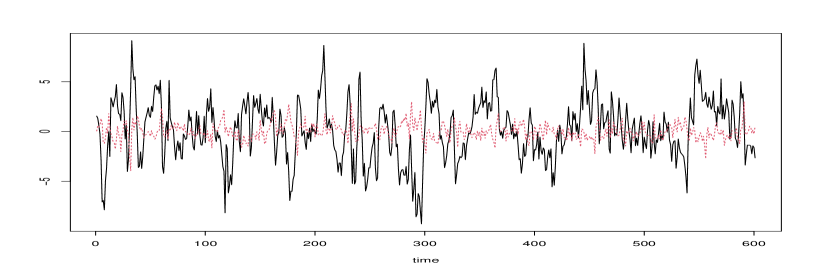
Figure 1: Trajectory of the Bivariate Causal-Noncausal VAR(1) Process: $Y_{1}$: solid line, $Y_{2}$: dashed line

The simulated paths of the series are displayed in Figure 1. The solid (black) line represents process $Y_{1t}$ and the dashed (red) line represents process $Y_{2t}$.

[Insert Figure 1: Trajectory of the Bivariate Causal-Noncausal VAR(1) Process]

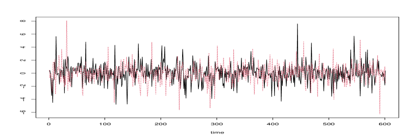
Figure 2: Trajectory of Error Processes: $\epsilon_{1}$: solid line, $\epsilon_{2}$: dashed line

We calculate the error series defined as $\varepsilon_{t}=Y_{t}-\Phi_{1}Y_{t-1}$. The two series are plotted in Figure 2. The sequence of bubbles is clearly visible in the noncausal component $Z_{2t}=Y_{2t}$ which impacts the component $Y_{1t}$ through the recursive form of matrix $\Phi$.

[Insert Figure 2: Trajectory of Error Processes]

The solid (black) line represents process $\varepsilon_{1}$ and the dashed (red) line represents process $\varepsilon_{2}$.

6.1.2 Nonlinear Forecast

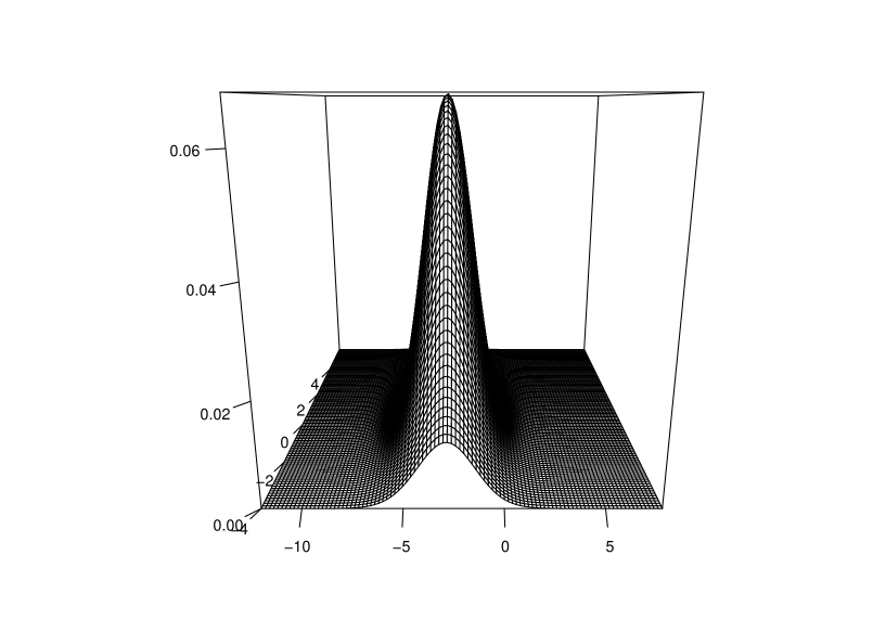
(a) Joint Predictive Density

(b) Marginal Predictive Density of $Y_{1,t}$

(c) Marginal Predictive Density of $Y_{2,t}$

Figure 3: Predictive Joint and Marginal Densities

Let us consider the nonlinear forecast at horizon 1 performed at date $T=590$. At time T=590, the process takes values -3.367 and -0.239. The true values of $Y_{1}$ and $Y_{2}$ at T+1=591 are -2.260 and -0.331, respectively. The nonlinear forecasts are summarized by the predictive density that can be used to compute the pointwise predictions of any nonlinear function of $Y_{1,T+1}$ and $Y_{2,T+1}$. The predictive bivariate density is given in Figure 3 along with the predictive marginal densities of $Y_{1,T+1}$ and $Y_{2,T+1}$, respectively .

[Insert Figure 3: Joint and Marginal Predictive Densities]

The predictive density provides the following point forecasts computed as the coordinates of the mode of the bivariate density. The point forecast of $Y_{1,591}$ is -2.80 and the point forecast of $Y_{2,591}$ is -0.50. The forecast intervals are determined from the predictive density: The forecast interval of $Y_{1,591}$ at level 0.90 is [-5.0, -1.0] and the forecast interval of $Y_{2,591}$ at level 0.90 is [-2.7, 2.1]. Both confidence intervals contain the true future values of the process.

We also perform 100 one-step-ahead forecasts along the trajectory, which are displayed in Figure 4. The RMSE for the two component processes are 1.414 and 1.381, respectively.

[Insert Figure 4: One-step Ahead Forecasts]

6.1.3 Nonlinear Forecast with GCov Estimated Parameters

The Generalized Covariance (GCov) estimate of matrix $\Phi$ is obtained by minimizing the portmanteau statistic computed from the auto- and cross-correlations up to and including lag $H=10$ of the errors $\varepsilon_{t}=Y_{t}-\Phi_{1}Y_{t-1}$ and their squared values [see Gourieroux, Jasiak (2017), (2021)] .

The following estimated autoregressive matrix is obtained:

$$\hat{\Phi}=\left(\begin{array}[]{cc}0.724&-1.452\\ -0.030&1.993\end{array}\right)$$

with eigenvalues $\lambda_{1}=0.690$, $\lambda_{2}=2.027$ close to the true values $J_{1}=0.7$ and $J_{2}=2.0$. The standard errors of $\hat{\Phi}$ obtained by bootstrap are 0.023, 0.308, for the elements of the first row, and 0.009, 0.120 for the elements of the second row.

After estimating $\Phi$, the GCov residuals $\hat{\varepsilon}_{t}=Y_{t}-\hat{\Phi}Y_{t-1}$ are computed and used for forecasting.

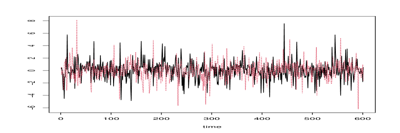
Figure 5: Trajectory of Residuals: $\hat{\epsilon}_{1}$: solid line, $\hat{\epsilon}_{2}$: dashed line

[Insert Figure 5: Trajectory of Residuals: $\hat{\varepsilon}_{1}$: solid line, $\hat{\varepsilon}_{2}$: dashed line ]

Matrices $A$ and $A^{-1}$ are identified from the spectral (Jordan) representation of matrix $\Phi$, up to scale factors. The estimated matrix $\hat{A}^{-1}$ computed from the normalized Jordan decomposition of $\hat{\Phi}$ is

$\hat{A}^{-1}=\left(\begin{array}[]{cc}0.022&0.025\\ -0.022&0.974\end{array}\right)$. It corresponds to matrix $A^{-1}=\left(\begin{array}[]{cc}1&1\\ 0&1\end{array}\right)$ up to scale factors of about 0.02 and 0.97 for each column.

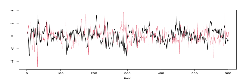
Figure 6: Trajectory of Components: $\hat{Z}_{1}$: solid line, $\hat{Z}_{2}$: dashed line

We use these estimates to approximate the causal and noncausal components displayed in Figure 6.

[Insert Figure 6: Trajectory of Components: $\hat{Z}_{1}$: solid line, $\hat{Z}_{2}$: dashed line ]

The point forecast of $Y_{1,591}$ based on the estimated parameters is -2.80 and the point forecast of $Y_{2,591}$ is -0.30. The forecast intervals at level 0.90 determined from the predictive density are as follows: The forecast interval of $Y_{1,591}$ at level 0.90 is [-4.80, -0.80] and the forecast interval of $Y_{2,591}$ is [-2.60, 2.10]. Both forecast intervals contain the true future values of the process.

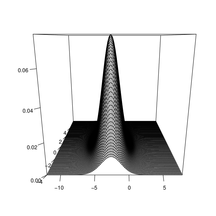
(a) Estimated Joint Predictive Density

(b) Estimated Marginal Predictive Density of $Y_{1,t}$

(c) Estimated Marginal Predictive Density of $Y_{2,t}$

Figure 7: Estimated Predictive Joint and Marginal Densities

[Insert Figure 7: Joint and Marginal Predictive Densities ]

The series of 100 one-step ahead forecasts along the trajectory is displayed in Figure 8.

[Insert Figure 8: Estimation-Based One-Step Ahead Forecasts]

The mean forecast error for $y_{1}$ is -0.035 and the RMSE for $y_{1}$ forecast is 1.453. The mean forecast error for $y_{2}$ is 0.102 and the RMSE for $y_{2}$ is 1.389.

6.2 Impulse Response Functions

This section illustrates steps 8-10 of the approach outlined in Section 5.

6.2.1 Causal innovation of the noncausal component (step 8)

The causal innovations $\hat{v}_{2,t}$ are obtained by applying formula (4.2) with$Z_{2,t}$ replaced by $\hat{Z}_{2,t}$, and by using the kernel estimate of the conditional c.d.f. $F_{2}$. The series of innovations $\hat{v}_{2,t}$ is given in Figure 9.

[Insert Figure 9: Innovation of Noncausal Component]

6.2.2 Link between the innovations (step 9)

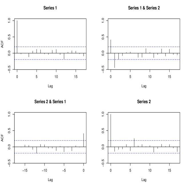
Figure 10: ACF of Innovations

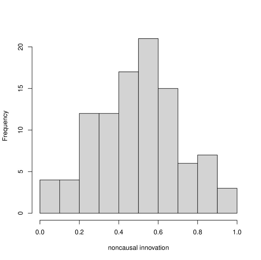
(b) Histogram of $v_{2,t}$

Figure 11: Innovation Histograms

We can now examine the joint dynamics of the innovations of causal and noncausal components $(\hat{\eta}_{1,t},\hat{v}_{2,t})$. Figure 10 shows the ACF and cross-ACF of these series and Figure 11 presents their histograms.

[Insert Figure 10: ACF of Innovations]

[Insert Figure 11: Innovation Histograms]

As pointed out in Section 4.3, if these series were independent, structural separate shocks could be applied to the causal and noncausal components. Then, the shock effects could be easily interpreted. In Figure 10, we see that the contemporaneous correlation is statistically significant. Therefore, the shock effects have to be interpreted by taking into account the existing simultaneity between $\eta_{1}$ and $v_{2}$.

6.2.3 Term structure of impulse responses (step 10)

The method for deriving the IRF outlined in Section 4.2 is applied as follows. The IRFs performed at date $T$ depend on:

- the scenario $s,s=1,...,S$, i.e. the i.i.d. draws in the joint distribution of $(\eta_{1,t},v_{2,t})$.

- the size of the shock at time $t$ and which innovation among $(\eta_{1,1},v_{2,1})$ the shock is applied to.

- the term $h$

Below, we illustrate the baseline and impulse responses of $Y_{1}$ and $y_{2}$ to a shock of size 0.3 applied to the noncausal innovation $v_{2,1}$ at time 1. The baseline innovations at h=2,…,30,are drawn from their historical distributions, except for fixed values of $\eta_{1,1}^{s}=0.0,v_{2,1}^{s}=0.5$ at time 1.

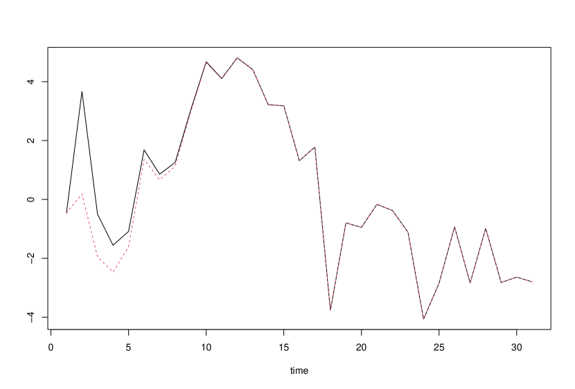
(a) Impulse Response of $y_{1}$

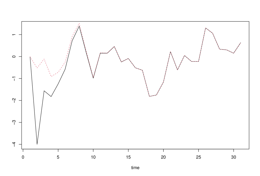
(b) Impulse Response of $y_{2}$

Figure 12: IRF to Shock of Size 0.3 to $v_{2,t}$; Baseline: black solid line, IRF: dashed red line

[Insert Figure 12: IRF to Shock of Size 0.3 to $v_{2,t}$]

We observe that $Y_{2}$ responds stronger to the shock than $Y_{1}$, while the shock effect to $Y_{2}$ is more long-lasting and dissipates at a slower rate.

In the next experiment, the shocks are independently and randomly drawn in the set $(\hat{\eta}_{1,t},\hat{v}_{2,t}),\;t=1,...,T$, i.e. in their historical distribution, with $\eta_{1,1}^{s}=0.0$ and $v_{2,1}^{s}=0.5$. The shocks $\delta=0.1,0.2,0.3$ are applied to innovation $v_{2,1}^{s}$. The benchmark value of $v_{2}$ is the median of the innovation distribution and the shocked values $v_{2}+\delta$ are the quantiles 0.6, 0.7, 0.8. The IRFs are computed for $h=1,...,H=10$ and replicated 200 times. For a given scenario and a given term, the IRF is a function of $\delta$. It is a nonlinear function of the shock size. By considering different scenarios, the term structure of IRF is obtained, which is shown to be random. It becomes a bivariate spatial process indexed by $(\delta,h)$.

The random term structure of IRF as a bivariate spatial process indexed by $(\delta,h)$ can be described in various ways. We focus on the marginal distribution of the differences between the simulated shocked and baseline values of $Y_{t+h}$, that is $Y_{t+h}^{s}(\delta)-Y_{t+h}^{s}$. Tables 1 and 2 provide the means, standard deviations and quantiles at 5% and 95% of the series $Y_{1}$ and $Y_{2}$, respectively.

In the standard causal VAR model, the IRF to a transitory shock at date $t$ tend rather quickly to 0 (when the eigenvalues of $\Phi$ are real positive and less than 1). In the mixed VAR model, the dissipation rate is different because the noncausal component can create nonlinear bubble effects. We observe that the mean IRF is a nonlinear function of $\delta$, in contrast to the causal VAR framework where that relation is linear.

Table 1: Impulse Response of $y_{1}$

h	baseline
	mean	s.dev.	q(5)	q(95)
1	-0.332	.	.	.
2	-0.175	2.054	-3.647	2.965
3	0.270	2.432	-3.820	4.511
4	0.605	2.786	-4.253	5.045
5	0.613	2.706	-4.008	4.802
6	0.620	2.939	-4.201	5.488
7	0.610	2.766	-3.834	5.068
8	0.508	2.667	-3.947	5.166
9	0.751	2.820	-4.305	5.050
10	0.700	2.899	-4.714	4.776
h	$\delta=0.1$
	mean	s.dev.	q(5)	q(95)
1	-0.596	.	.	.
2	-0.469	1.994	-4.035	2.538
3	0.0904	2.447	-3.804	4.074
4	0.247	2.486	-3.840	4.188
5	0.244	2.659	-3.972	4.395
6	0.110	2.548	-4.001	4.358
7	0.407	2.510	-3.656	4.756
8	0.561	2.717	-3.598	5.472
9	0.496	2.712	-3.688	4.875
10	0.183	2.700	-4.162	4.565
h	$\delta=0.2$
	mean	s.dev.	q(5)	q(95)
1	-0.868	.	.
2	-0.681	2.001	-3.734	2.564
3	-0.085	2.236	-3.623	3.809
4	0.191	2.663	-4.398	4.147
5	0.332	2.544	-3.616	4.694
6	0.319	2.765	-4.422	5.038
7	0.433	2.814	-4.651	4.748
8	0.459	2.816	-4.217	4.997
9	0.139	2.862	-4.426	4.492
10	0.171	2.871	-4.116	4.800
h	$\delta=0.3$
	mean	s.dev.	q(5)	q(95)
1	-1.196	.	.
2	-0.815	1.973	-4.036	2.490
3	-0.413	2.477	-4.451	3.991
4	-0.001	2.620	-4.678	4.073
5	0.252	2.805	-4.240	4.842
6	0.544	2.776	-3.268	5.294
7	0.530	2.774	-3.797	4.949
8	0.743	2.698	-3.849	4.880
9	0.719	2.850	-3.916	4.866
10	0.697	2.967	-3.740	5.400

Table 2: Impulse Response of $y_{2}$

h	baseline
	mean	s.dev.	q(5)	q(95)
1	0.0	.	.	.
2	0.024	1.002	-1.528	1.592
3	-0.064	1.222	-1.968	1.888
4	-0.065	1.239	-2.000	1.728
5	-0.035	1.322	-2.480	2.120
6	-0.011	1.322	-2.200	2.208
7	-0.040	1.395	-2.504	2.200
8	0.024	1.343	-2.224	2.160
9	0.010	1.318	-2.208	2.216
10	-0.084	1.251	-2.000	2.128
h	$\delta=0.1$
	mean	s.dev.	q(5)	q(95)
1	0.264	.	.	.
2	0.277	1.066	-1.472	1.992
3	0.077	1.158	-1.952	1.912
4	-0.043	1.256	-2.016	1.936
5	0.035	1.281	-2.136	2.176
6	0.153	1.187	-1.712	2.176
7	0.042	1.256	-1.840	2.040
8	0.055	1.307	-2.248	2.152
9	0.247	1.238	-1.984	2.032
10	0.286	1.255	-1.848	2.344
h	$\delta=0.2$
	mean	s.dev.	q(5)	q(95)
1	0.536	.	.	.
2	0.368	1.010	-1.424	1.928
3	0.233	1.166	-1.912	2.096
4	0.137	1.251	-2.224	1.856
5	0.071	1.266	-1.888	2.240
6	-0.040	1.316	-2.336	2.192
7	-0.119	1.352	-2.248	2.232
8	-0.034	1.310	-2.136	2.024
9	0.012	1.283	-2.344	2.008
10	-0.070	1.311	-2.456	2.120
h	$\delta=0.3$
	mean	s.dev.	q(5)	q(95)
1	0.864	.	.	.
2	0.664	0.955	-0.920	2.224
3	0.468	1.248	-1.400	2.656
4	0.155	1.296	-1.888	2.248
5	0.043	1.305	-2.096	2.080
6	-0.083	1.297	-2.232	1.992
7	0.080	1.268	-1.976	2.280
8	-0.115	1.269	-2.336	2.224
9	-0.084	1.303	-2.192	2.032
10	-0.096	1.221	-2.200	2.016

6.3 Application to Cryptocurrency Prices

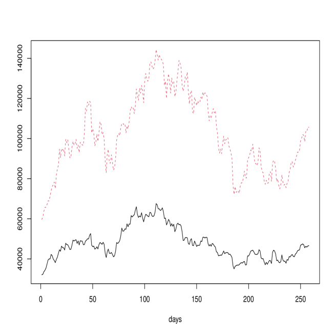
Figure 13: BTC/USD and ETH/USD Daily Closing Rates, July 21, 2021 to April 04, 2022 BTC/USD: solid black line, ETH/USD (times 30): dashed red line

This section examines the bivariate series of Bitcoin and Ethereum prices in US Dollars. The Bitcoin (BTC) and Ethereum (ETH) are the main cryptocurrencies with market capitalizations of about 765 and 364 trillions of Dollars, respectively. The bivariate series of 257 daily adjusted closing BTC/USD and ETH/USD exchange rates recorded between July 21, 2021 and April, 04, 2022 are displayed in Figure 13:

[Insert Figure 13: BTC/USD and ETH/USD Daily Closing Rates]

We observe that both series display comovements over time and their dynamics are characterized by spikes and local trends/bubbles.

The bivariate VAR model is estimated from the data rescaled and adjusted by a polynomial function of time of order 2 for the hump-shaped pattern in the middle of the sampling period. The estimation is performed without imposing any distributional assumptions on the errors. We use the semi-parametrically efficient GCov estimator with nonlinear transformations including powers two, three and four of the errors summed up to lag 10. The estimated matrix $\hat{\Phi}$ is:

$$\hat{\Phi}=\left(\begin{array}[]{cc}-0.0901&1.1998\\ 0.4183&0.7724\end{array}\right),$$

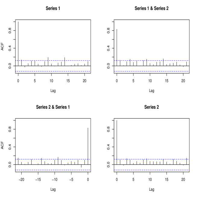
Figure 14: Residual ACF

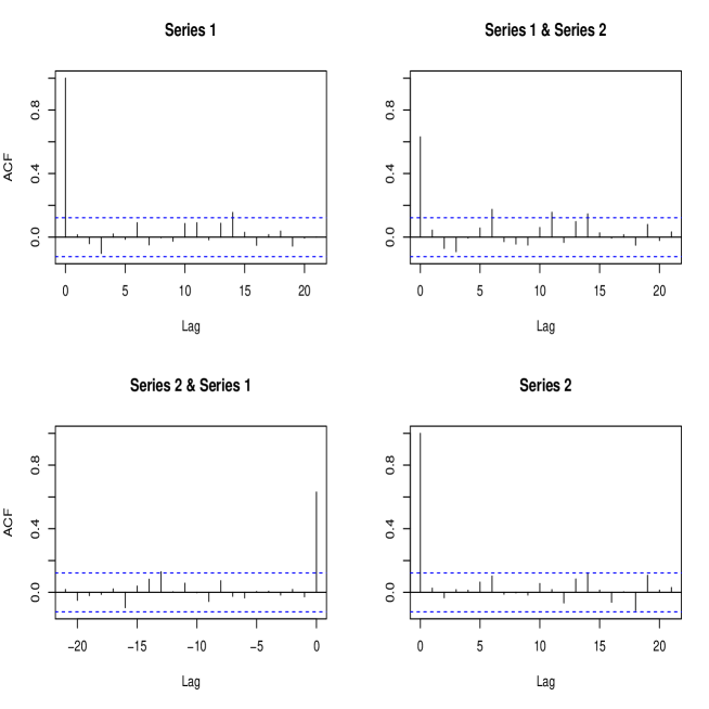
Figure 15: ACF of Squared Residuals

with eigenvalues -0.488 and 1.171. Hence, there is a single noncausal component that captures the codependent successive bubbles observed in Figure 13. The standard errors of $\hat{\Phi}_{1,1}$ and $\hat{\Phi}_{1,2}$ are 0.014 and 0.013. For $\hat{\Phi}_{2,1}$ and $\hat{\Phi}_{2,2}$ the standard errors take values 0.022 and 0.019, respectively. Figures 14 and 15 display the autocorrelations of the residuals and squared residuals of the VAR(1) model indicating that the residuals are close to a bivariate white noise and the model provides a satisfactory fit.

[Insert Figure 14: Residual ACF]

[Insert Figure 15: ACF of Squared Residuals]

The Jordan decomposition of matrix $\hat{\Phi}$ is:

$$\hat{\Phi}=\hat{A}\hat{J}\hat{A}^{-1}$$

with

$\hat{A}=\left(\begin{array}[]{cc}-3.013&0.951\\ 1&1\end{array}\right)$, $\hat{J}=\left(\begin{array}[]{cc}-0.488&0\\ 0&1.171\end{array}\right)$, $\hat{A}^{-1}=\left(\begin{array}[]{cc}-0.252&0.240\\ 0.252&0.759\end{array}\right)$.

We forecast the adjusted closing BTC/USD and ETH/USD exchange rates on April 4, 2022 equal to 46622.67 and 3521.24, respectively. The point forecast of demeaned and rescaled $y_{1,T+1}$ is -740.00, and the forecast of demeaned $y_{2,T+1}$ is 105.00. The forecast interval of $y_{1}$ at 0.90% is [-940.00 and -150.00] and contains the true value -844.81. The forecast interval of $y_{2}$ at 0.90% is [57.00, 174.00] and contains the true value 126.68. After adjusting for the mean and scale, we obtain forecasts of 46727.0 for Bitcoin and 3499.56 for Ethereum prices, which are off by 105 and 22 Dollars, respectively, outperforming a combined ”no-change” forecast based on the previous day values.

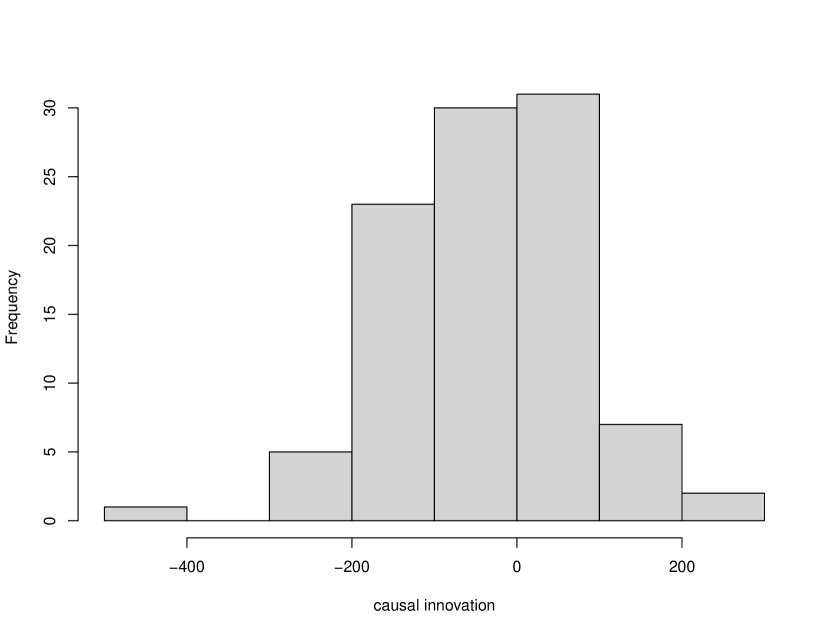
(a) Histogram of $v_{1,t}$

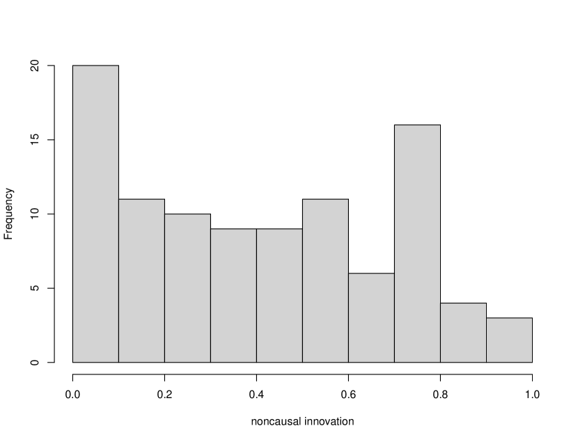
(b) Histogram of $v_{2,t}$

Figure 16: Innovation Histograms

The histograms of nonlinear innovations are presented in Figure 16.

[Insert Figure 16: Innovation Histograms]

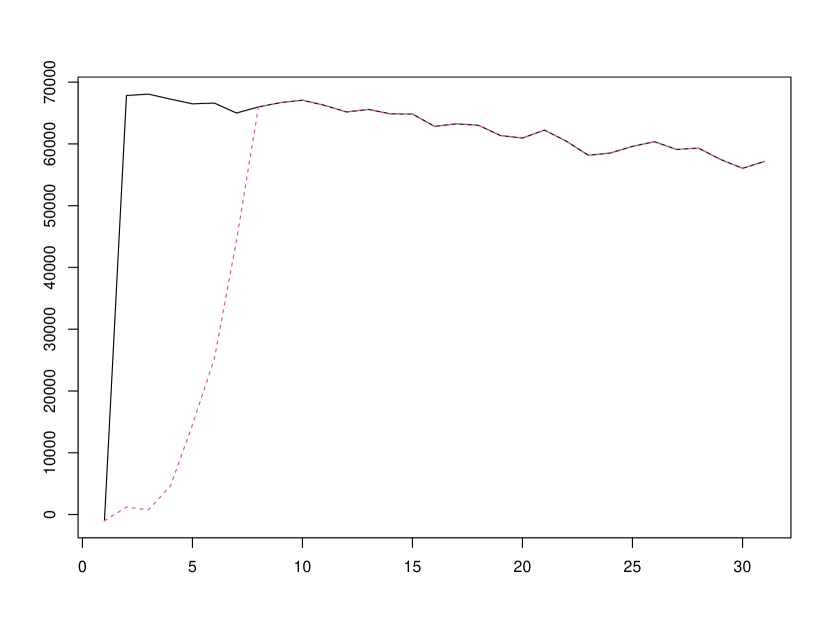
(a) Impulse Response of Demeaned $y_{1}$

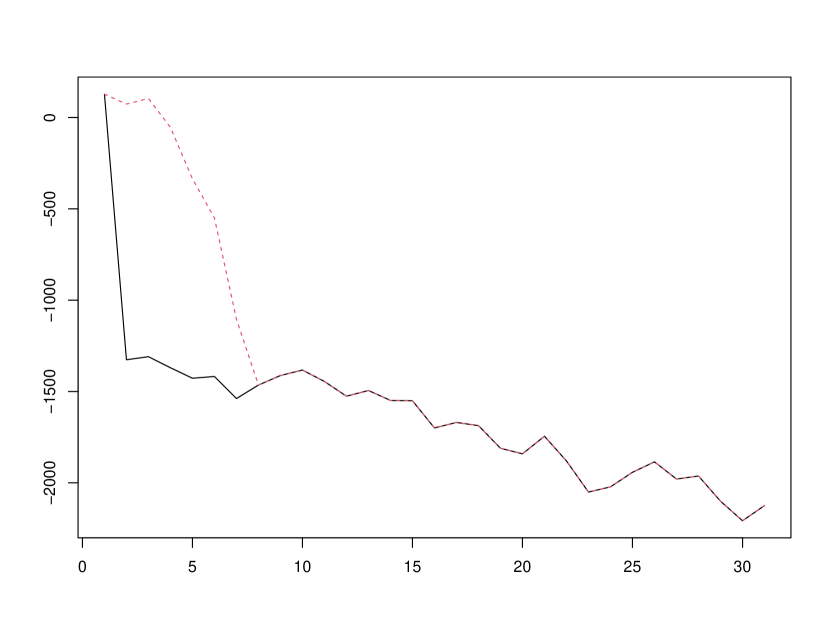
(b) Impulse Response of Demeaned $y_{2}$

Figure 17: IRF to Shock of Size 0.3 to $v_{2,t}$; Baseline: black solid line, IRF: dashed red line

The histogram of $v_{1}$ reveals a close to symmetric density with a long left tail, while the histogram of $v_{2}$ is close to a uniform density shape. Following the approach outlined in Section 6.2, we evaluate the impulse responses of adjusted data to a shock of size 0.3 to $v_{2,1}$. The baseline is equal to 30 values of the causal and noncausal innovations drawn in their historical distributions. The impulse response functions are plotted in Figure 17.

[Insert Figure 17: Impulse Responses]

The shocks to Bitcoin and ETH rates have about the same duration of 8 periods(days) before dissipating fully, and generate strong responses in both series.

7 Concluding Remarks

This paper examines nonlinear forecast and impulse response functions (IRF) in the framework of a causal-noncausal (S)VAR model. It provides the closed-form expression of the (causal) predictive distribution of the VAR model and introduces (past-dependent) causal nonlinear innovations. As the causal nonlinear innovations are not uniquely defined, their identification is examined in detail. We show how the stochastic term structure of IRF can be computed, from selected causal nonlinear innovations.

The approach is illustrated by a simulation study highlighting the differences between the errors, residuals and innovations of a mixed (S)VAR model. The proposed approach is applied to cryptocurrency prices providing nonlinear forecast and impulse response functions.

R E F E R E N C E S

Bec, F., Nielsen, H. and S. Saidi (2020): ”Mixed Causal-Noncausal Autoregression: Bimodality Issues in Estimation and Unit Root Testing”, Oxford Bulletin of Economics and Statistics, 82, 1413-1428.

Blanchard, O. and D. Quah (1989): ”The Dynamic Effects of Aggregate Demand and Supply Disturbances”, American Economic Review, 79, 655-673.

Breidt, F., Davis, R., Lii, K. and M. Rosenblatt (1991) : ”Maximum Likelihood Estimation for Noncausal Autoregressive Processes”, Journal of Multivariate Analysis, 36, 175-198.

Cambanis, S. and I. Fakhre-Zakeri (1994): ”On Prediction of Heavy-Tailed Autoregressive Sequences Forward versus Reversed Time, Theory of Probability and its Applications, 39, 217-233.

Chan, K., Ho, L. and H. Tong (2006) : ”A Note on Time-Reversibility of Multivariate Linear Processes”, Biometrika, 93, 221-227.

Cochrane, J. (1994): ”Shocks”, Carnegie-Rochester Conference Series on Public Policy”, 41, 295-324.

Christiano, L, Eichenbaum, M. and C. Evans (1996): ”The Effects of Monetary Policy Shocks: Evidence from the Flow of Funds”, Review of Economics and Statistics, 78, 16-34.

Comon, P. (1994): ”Independent Component Analysis: A New Concept?”, Signal Process., 36, 287-314.

Cordoni, F. and F. Corsi (2019): ”Identification of Singular and Noisy Structural VAR Models: The Collapsing ICA Approach”, D.P. University of Pisa.

Davis, R. and L. Song (2020) : ”Noncausal Vector AR Processes with Application to Economic Time Series”, Journal of Econometrics, 216, 246-267.

Eriksson, J. and V. Koivunen (2004): ”Identifiability, Separability and Uniqueness of Linear ICA Models”, IEEE Signal Processing Letter, 11, 601-604.

Faust, J. and E. Leeper (1997): ”When Do Long Run Identifying Restrictions Give Reliable Results”, Journal of Business and Economic Statistics, 15, 345-353.

Funovits, B. and J. Nyholm (2016): ”Multivariate All-Pass Time Series Models: Modelling and Estimation Strategies”, D.P. University of Helsinki

Gelfand, A. and A. Smith (1992): ”Bayesian Statistics without Tears: A Sampling-Resampling Perspective”, Annals of Statistics, 46, 84-88.

Gonzalves, S., Herrera, A., Kilian, L. and E. Pesavento (2021): ’Impulse Response Analysis for Structural Dynamic Models with Nonlinear Regressors”, Journal of Econometrics, 225, 107-130.

Gonzalves, S., Herrera, A., Kilian, L. and E. Pesavento (2022): ”When Do State-dependent Local Projections Work?”, McGill U, working paper.

Gourieroux, C. and A. Hencic (2015) : ”Noncausal Autoregressive Model in Application to Bitcoin/USD Exchange Rates”, Econometrics of Risk, Studies in Computational Intelligence, 583:17-40

Gourieroux, C. and J. Jasiak (2005) : ”Nonlinear Innovations and Impulse Responses with Application to VaR Sensitivity”, Annals of Economics and Statistics, 78, 1-31.

Gourieroux, C. and J. Jasiak (2016): ”Filtering, Prediction, and Simulation Methods for Noncausal Processes”, Journal of Time Series Analysis, 37, 405-430.

Gourieroux, C. and J. Jasiak (2017): ”Noncausal Vector Autoregressive Process: Representation, Identification and Semi-Parametric Estimation”, Journal of Econometrics, 200, 118-134.

Gourieroux, C. and J. Jasiak (2021): ”Generalized Covariance Estimator”, CREST.

Gourieroux, C., Monfort, A. and J.P. Renne (2017) : ”Statistical Inference for Independent Component Analysis”, Application to Structural VAR Models”, Journal of Econometrics, 196, 111-126.

Gourieroux, C., Monfort A. and J.P. Renne (2020): ”Identification and Estimation in Nonfundamental Structural VARMA Models”, Review of Economic Studies, 87, 1915-1953.

Gourieroux, C. and J.M. Zakoian (2017) : ”Local Explosion Modelling by Noncausal Process”, Journal of the Royal Statistical Society, B, 79, 737-756.

Granzeria, E., Moon, H. and F., Schorfheide (2018): ”Inference for VARs Identified with Sign Restrictions”, Quantitative Economics, 9, 1087-1121.

Guay, A. (2021): ”Identification of Structural Vector Autoregressions Through Higher Unconditional Moments”, Journal of Econometrics, 225, 27-45.

Hamilton, J. (1994): ”Time Series Analysis”, Princeton, New Jersey.

Hecq, A. , Lieb, L. and S. Telg (2016): ”Identification of Mixed Causal-Noncausal Models in Finite Samples”, Annals of Economics and Statistics, 123/124, 307-331.

Keweloh, S. (2021): ”A Generalized Method of Moments Estimator for Structural Vector Autoregressions Based on Higher Moments”, Journal of Business and Economic Statistics, 39, 772-782.

Koop, G., Pesaran, H. and S. Potter (1996): ”Impulse Response Analysis in Nonlinear Multivariate Models”, Journal of Econometrics, 74, 119-147.

Lanne, M. and J. Luoto (2021): ”GMM Estimation of Non-Gausian Structural Vector Autoregressions”, Journal of Business and Economic Statistics, 39, 69-81.

Lanne, M., Luoto J. and P. Saikkonen (2012) : ’Optimal Forecasting of Noncausal Autoregressive Time Series”, International Journal of Forecasting, 28, 623-631.

Lanne, M. and P. Saikkonen (2008): ”Modelling Expectations with Noncausal Autoregressions”, European University Institute, D.P. 2008/20.

Lanne, M. and P. Saikkonen (2010) : ”Noncausal Autoregressions for Economic Time Series”, Journal of Time Series Econometrics, 3, 1-39.

Lanne, M. and P. Saikkonen (2011) : ”GMM Estimators with Non-Causal Instruments”, Oxford Bulletin of Economics and Statistics, 71, 581-591.

Lanne, M. and P. Saikkonen (2013) : ”Noncausal Vector Autoregression”, Econometric Theory, 29, 447-481.

Leeper, E., Walker, T. and S. Yang (2013) : ”Fiscal Foresight and Information Flows”, Econometrica, 81, 1115-1145.

Lutkepohl, H. (1990): ”Asymptotic Distribution of Impulse Response Functions and Forecast Error Variance Decomposition of Vector Autoregressive Models”, Review of Economics and Statistics, 72, 116-125.

Nyberg, H. and P. Saikkonen (2014): ’Forecasting with a Noncausal VAR Model”, Computational Statistics and Data Analysis, 76, 536-555.

Perko, L. (2001): ”Differential Equations and Dynamical Systems”, Springer, New York.

Potter, S. (2000): ”Nonlinear Impulse Response Functions”, Journal of Economic Dynamics and Control, 24, 1425-1426.

Rosenblatt, M. (2012) : ”Gaussian and Non-Gaussian Linear Time Series and Random Fields”, Springer Verlag.

Rubio-Ramirez, J. F., Waggoner, D. F. and T. Zha, (2010): ”Structural Vector Autoregressions: Theory of Identification and Algorithms for Inference”, Review of Economic Studies, 77, 665-696.

Sims, C. (1980): ”Macroeconomics and Reality”, Econometrica, 48, 1-48.

Sims, C. (2002): ”Structural VAR’s”, Econ 513, Time Series Econometrics, Princeton.

Swensen, A. (2022): ”On Causal and Non-Causal Cointegrated Vector Autoregressive Time Series”, Journal of Time Series Analysis, 42, 178-196.

Tanner, M. (1993): ”Tools for Statistical Inference”, Springer Series in Statistics, 2nd edition, Springer, New York.

Uhlig, H. (2005): ”What are the Effects of Monetary Policy on Output? Result from an Agnostic Identification Procedure”, Journal of Monetary Economics, 52, 381-419.

Velasco, C. (2022): ”Identification and Estimation of Structural VARMA Models Using Higher Order Dynamics”, Journal of Business and Economic Statistics, forthcoming.

Velasco, C., and I. Lobato (2018): ”Frequency Domain Minimum Distance Inference for Possibly Noninvertible and Noncausal ARMA Models”, Annals of Statistics, 46, 555-579.

(a) Forecasts of $Y_{1,t}$

(b) Forecasts of $Y_{2,t}$

Figure 4: One-step Ahead Forecasts

(a) Estimation-Based Forecasts of $Y_{1,t}$

(b) Estimation-Based Forecasts of $Y_{2,t}$

Figure 8: Estimation-Based One-Step Ahead Forecasts true:solid line, forecast:dashed line

Figure 9: Innovation of Noncausal Component

(a) Histogram of $v_{1,t}=\eta_{1,t}$

APPENDIX 1

Proof of Proposition 1

The proof follows the same lines as in Gourieroux, Jasiak (2016), (2017).

1) Let us consider the information set:

$$I_{T+1}=(Y_{1},...,Y_{T},Y_{T+1}).$$

This set is equivalent to the set generated by $(Z_{1},Z_{2},...,Z_{T+1})$ and the set generated by $(Z_{1,2},\eta_{3},\eta_{4},....,\eta_{T},\eta_{1,T+1},Z_{2,T},Z_{2,T+1})$ by using the recursive equations (3.10). Since $(\eta_{1,T+1},Z_{2,T},Z_{2,T+1})$ is independent of $\underline{\varepsilon}_{T}$, we see that the conditional density $l(\eta_{1,T+1},Z_{2,T},Z_{2,T+1}|\underline{\varepsilon}_{T})=l(\eta_{1,T+1},Z_{2,T},Z_{2,T+1})$ is equal to the marginal density.

It follows that the conditional density is:

$$l(\eta_{1,T+1},Z_{2,T+1}|Z_{2,T},\underline{\varepsilon}_{T})=l(\eta_{1,T+1},Z_{2,T+1}|I_{T})=l(\eta_{1,T+1},Z_{2,T+1}|Z_{2,T}).$$ (a.1)

The last conditional density needs to be rewritten with a conditioning variable being the future $Z_{2}$. From the Bayes theorem, it follows that:

$$l(\eta_{1,T+1},Z_{2,T+1}|I_{T})=\frac{l_{2}(Z_{2,T+1})}{l_{2}(Z_{2,T})}\;l(\eta_{1,T+1},Z_{2,T}|Z_{2,T+1}),$$ (a.2)

where $l_{2}$ is the marginal density of $Z_{2,t}$.

2) Let us now consider the vector $\eta_{t}=A^{-1}\left(\begin{array}[]{c}\varepsilon_{t}\\ 0\end{array}\right)$. This random vector takes values on the subspace $E=A^{-1}(I\hskip-3.0ptR^{m}\times I\hskip-3.0ptR^{n-m})$. Its distribution admits a density $g_{\eta}(\eta_{1},\eta_{2})$ with respect to the Lebesgue measure on subspace $E$. Moreover, we have:

$$\eta_{T+1}=\left(\begin{array}[]{c}\eta_{1,T+1}\\ Z_{2,T+1}-J_{2}Z_{2,T}\end{array}\right)=\left(\begin{array}[]{cc}Id&0\\ 0&-J_{2}\end{array}\right)\left(\begin{array}[]{c}\eta_{1,T+1}\\ Z_{2,T}\end{array}\right)+\left(\begin{array}[]{c}0\\ Z_{2,T+1}\end{array}\right).$$ (a.3)

Then, conditional on $Z_{2,T+1}$, vector $\left(\begin{array}[]{c}\eta_{1,T+1}\\ Z_{2,T}\end{array}\right)$ takes values in the affine subspace $F=\left(\begin{array}[]{cc}Id&0\\ 0&-J_{2}\end{array}\right)^{-1}\left[E-\left(\begin{array}[]{c}0\\ Z_{2,T+1}\end{array}\right)\right]$ with a density with respect to the Lebesgue measure on $F$. Since the transformation from $\eta_{T+1}$ to $\left(\begin{array}[]{c}\eta_{1,T+1}\\ Z_{2,T}\end{array}\right)$ is linear affine invertible, we can apply the Jacobian formula to get:

$$l(\eta_{1,T+1},Z_{2,T}|Z_{2,T+1})=|\det J_{2}|\,g_{\eta}(\eta_{1,T+1},Z_{2,T+1}-J_{2}Z_{2,T}).$$ (a.4)

Then from (a.2), (a.4) and $Z_{1,T+1}=J_{1}Z_{1,T}+\eta_{1,T+1}$, it follows that:

$$l(Z_{1,T+1},Z_{2,T+1}|I_{T})=\frac{l_{2}(Z_{2,T+1})}{l_{2}(Z_{2,T})}\;|\det J_{2}|\,g_{\eta}(Z_{1,T+1}-J_{1}Z_{1,T},Z_{2,T+1}-J_{2}Z_{2,T}).$$ (a.5)

Let us now derive the predictive density of $Y_{T+1}$ given $I_{T}$. We get a succession of affine transformations of variables with values in different affine subspaces (depending on the conditioning set) along the following scheme:

$$\begin{array}[]{ccccccc}\left(\begin{array}[]{c}\varepsilon_{T+1}\\ 0\end{array}\right)&\stackrel{{\scriptstyle A^{-1}}}{{\rightarrow}}&\eta_{T+1}&\stackrel{{\scriptstyle Id}}{{\rightarrow}}&Z_{T+1}&\stackrel{{\scriptstyle A}}{{\rightarrow}}&\left(\begin{array}[]{c}Y_{T+1}\\ \tilde{Y}_{T}\end{array}\right).\\ &&&&(\mbox{given}\;Z_{T})&&(\mbox{given}\;\tilde{Y}_{T})\end{array}$$

Then, we can apply three times the Jacobian formula on manifolds. Since $|\det A^{-1}||\det A|=\frac{|\det A|}{|\det A|}=1$, the Jacobians cancel out and the predictive density becomes:

$$l(y|\underline{Y}_{T})=\frac{l_{2}\left[A^{2}\left(\begin{array}[]{c}y\\ \tilde{Y}_{T-1}\end{array}\right)\right]}{l_{2}\left[A^{2}\left(\begin{array}[]{c}Y_{T}\\ \tilde{Y}_{T-1}\end{array}\right)\right]}\,|\det J_{2}|\,g(y-\Phi_{1}Y_{T}-\cdots-\Phi_{p}Y_{T-p+1}),$$

which yields the formula in Proposition 1.

APPENDIX 2

The Causal-Noncausal Model in Multiplicative Form

The multiplicative causal-noncausal model is:

$$\Phi(L)\Psi(L^{-1})Y_{t}=\varepsilon^{*}_{t},$$

where both autoregressive polynomials have roots outside the unit circle and i.i.d. errors $\varepsilon^{*}_{t}$. This model is used in Lanne, Luoto, Saikkonen (2012), Lanne, Saikkonen (2013) and Nyberg, Saikkonen (2014). While the multiplicative representation is equivalent to the general AR(p) model for univariate time series, it is not the case in the multivariate framework.

As pointed out in Davis, Song (2020), p. 247, this decomposition implies restrictions on the autoregressive coefficients $\Phi_{1},...,\Phi_{p}$ of the past-dependent representation.

Moreover, it is not compatible with the SVAR specification (2.1). To illustrate this problem, let us consider the multiplicative bivariate model:

$$\left(\begin{array}[]{cc}1-\phi L&0\\ 0&1\end{array}\right)\left(\begin{array}[]{cc}1&0\\ 0&1-\psi L^{-1}\end{array}\right)Y_{t}=\varepsilon_{t}^{*}.$$

It follows that:

$$Y_{1,t}-\phi Y_{1,t-1} = \varepsilon_{1,t}^{*},$$

$$Y_{2,t}-\psi Y_{2,t+1} = \varepsilon_{2,t}^{*},$$

or equivalently:

$$Y_{1,t}-\phi Y_{1,t-1} = \varepsilon_{1,t}^{*},$$

$$Y_{2,t}-\frac{1}{\psi}Y_{2,t-1} = -\frac{1}{\psi}\varepsilon_{2,t-1}^{*},$$

$$\iff Y_{t}=\left(\begin{array}[]{cc}\phi&0\\ 0&\frac{1}{\psi}\end{array}\right)Y_{t-1}+\varepsilon_{t},$$

where $\varepsilon_{t}=\left(\begin{array}[]{c}\varepsilon_{1,t}\\ \varepsilon_{2,t}\end{array}\right)$ with $\varepsilon_{1,t}=\varepsilon_{1,t}^{*}$ and $\varepsilon_{2,t}=-\frac{1}{\psi}\varepsilon_{2,t-1}^{*}$.

We observe that, if $\varepsilon_{1,t}^{*},\varepsilon_{2,t}^{*}$ are correlated, then $\varepsilon_{1,t}$ and $\varepsilon_{2,t+1}$ are correlated too. Therefore the condition of i.i.d. errors in the SVAR model (2.1) cannot be satisfied.

This major difficulty is a consequence of a different normalization. For example, if $\Phi(L)=Id-\Phi L$ and $\Psi(L^{-1})=Id-\Psi L^{-1}$, then the multiplicative model is such that:

$$\Phi(L)\Psi(L^{-1})Y_{t}=-\Psi Y_{t+1}+(Id+\Phi\Psi)Y_{t}-\Phi Y_{t-1}=\epsilon_{t}^{*},$$

which cannot be transformed into:

$$Y_{t}=\Phi_{1}Y_{t-1}+\Phi_{2}Y_{t-2}+\varepsilon_{t},$$

if matrix $\Psi$ is not invertible.

APPENDIX 3

Identification of Nonlinear Causal Innovations

For ease of exposition, let us consider a bivariate VAR(1) model, which is a Markov process. By analogy to the recursive (i.e. causal) approach for defining the shocks, we start from the first component.

i) Let $F_{1}[y_{1}|Y_{T-1}]$ denote the conditional c.d.f. of $Y_{1,T}$ given $Y_{T-1}$ and define:

$$v_{1,T}=F_{1}[Y_{1,T}|Y_{T-1}].$$ (a.6)

Then, $v_{1,T}$ follows a uniform distribution $U_{[0,1]}$ for any $Y_{T-1}$. In particular, $v_{1,T}$ is independent of $Y_{T-1}$.

ii) Let $F_{2}[y_{2}|Y_{1,T},Y_{T-1}]$ denote the conditional c.d.f. of $Y_{2,T}$ given $Y_{1,T},Y_{T-1}$, and define:

$$v_{2,T}=F_{2}[Y_{2,T}|Y_{1,T},Y_{T-1}].$$ (a.7)

It follows that $v_{2,T}$ follows a uniform distribution on [0,1], for any $Y_{1,T},Y_{T-1}$, or equivalently for any $v_{1,T},Y_{T-1}$. Therefore, $v_{2,T}$ is independent of $v_{1,T},Y_{T-1}$.

iii) By inverting equations (a.6)-(a.7), we obtain a nonlinear autoregressive representation: $Y_{T}=g(Y_{T-1},v_{T})$, where the $v_{T}$’s are i.i.d. such that $(v_{1,T}),(v_{2,T})$ are independent.

Clearly, this brings us back to the standard shock identification issue, called the Wold causality ordering, encountered in linear Gaussian models. Indeed, the same approach can be applied to the alternative ordering: $Y_{2,T}$ followed by $Y_{1,T}$ given $Y_{2,T}$. More generally, for any invertible nonlinear transformation $Y_{T}^{*}=c(Y_{T})$, the above approach can be applied first to $Y_{1,T}^{*}$ and next to $Y_{2,T}^{*}$ conditional on $Y_{1,T}^{*}$.

Let us now describe in detail all the identification issues. First, we can assume that $v_{1,T},v_{2,T}$ are i.i.d and independent of one another with uniform distributions on [0,1]. We need to find out if there exists another pair of variables $w_{1,T},w_{2,T}$, which are independent and uniformly distributed such that:

$$g(Y_{T-1},w_{T})=g(Y_{T-1},v_{T}),\;\;\forall Y_{T-1},$$

or, equivalently, a pair of variables $w_{T}$ that satisfy a (nonlinear) one-to-one relationship with $v_{T}$. Let $w=a(v)$ denote this relationship. We have the following Lemma:

Lemma A.1:

Let us assume that $a$ is continuous, twice differentiable and that the Jacobian matrix $\partial a(v)/\partial v$ has distinct eigenvalues. Then, the components of $a$ are harmonic functions, that is:

$$\frac{\partial^{2}a_{j}(v)}{\partial v_{1}^{2}}+\frac{\partial^{2}a_{j}(v)}{\partial v_{2}^{2}}=0,\;\;j=1,2.$$

Proof:

i) We can apply the Jacobian formula to get the density of $w$ given the density of $v$. Since both joint densities are uniform, it follows that $|\det\frac{\partial a(v)}{\partial v}|=1$, $\forall v\in[0,1]^{2}$.

ii) Let us consider the eigenvalues $\lambda_{1}(v),\lambda_{2}(v)$ of the Jacobian matrix $\frac{\partial a(v)}{\partial v}$. The eigenvalues are continuous functions of this matrix, and therefore continuous functions of $v$ (whenever these eigenvalues are different). Then, two cases can be distinguished:

case 1: The eigenvalues are real.

case 2: The eigenvalues are complex conjugates.

iii) In case 1, we have $\lambda_{2}(v)=1/\lambda_{1}(v)$ ( or $-1/\lambda_{1}(v)$), where $\lambda_{1}(v)$ is less or equal to 1 in absolute value for any $v$, and then $\lambda_{2}(v)$ is larger than or equal to 1 in absolute value for any $v$. Since $a(v)\in[0,1]^{2}$ for any $v\in[0,1]^{2}$, it follows that $\lambda_{2}(v)$ cannot be explosive.

iv) Therefore case 2 is the only relevant one. Let us consider the case $\det\frac{\partial a(v)}{\partial v}=1$, $\forall v\in[0,1]^{2}$ (the analysis of $\det\frac{\partial a(v)}{\partial v}=-1$ is similar). Then, the Jacobian matrix is a rotation matrix:

$$\frac{\partial a(v)}{\partial v}=\left(\begin{array}[]{cc}\frac{\partial a_{1}(v)}{\partial v_{1}}&\frac{\partial a_{1}(v)}{\partial v_{2}}\\ \frac{\partial a_{2}(v)}{\partial v_{1}}&\frac{\partial a_{2}(v)}{\partial v_{2}}\end{array}\right)\equiv\left(\begin{array}[]{cc}\cos\theta(v)&-\sin\theta(v)\\ \sin\theta(v)&\cos\theta(v)\end{array}\right).$$

We deduce that:

$$\frac{\partial a_{1}(v)}{\partial v_{1}} = \frac{\partial a_{2}(v)}{\partial v_{2}},$$

$$\frac{\partial a_{1}(v)}{\partial v_{2}} = -\frac{\partial a_{2}(v)}{\partial v_{1}}.$$ (a.8)

Let us differentiate the first equation with respect to $v_{1}$ and the second one with respect to $v_{2}$. We get:

$$\frac{\partial^{2}a_{1}(v)}{\partial v_{1}^{2}}=\frac{\partial^{2}a_{2}(v)}{\partial v_{1}\partial v_{2}}\;\;\mbox{and}\;\;\frac{\partial^{2}a_{1}(v)}{\partial v_{2}^{2}}=-\frac{\partial^{2}a_{2}(v)}{\partial v_{1}\partial v_{2}},$$ (a.9)

and by adding these equalities:

$$\frac{\partial^{2}a_{1}(v)}{\partial v_{1}^{2}}+\frac{\partial^{2}a_{1}(v)}{\partial v_{2}^{2}}=0.$$ (a.10)

Therefore $a_{1}$ is a harmonic function that satisfies the Laplace equation. Similarly, $a_{2}$ is also a harmonic function. QED

Harmonic functions are regular functions: they are infinitely differentiable and have series representations that can be differentiated term by term [Axler et al. (2001)]:

$$a_{1}(v) = \sum_{h=0}^{\infty}\sum_{k=0}^{\infty}(a_{1hk}v_{1}^{k}v_{2}^{h}),$$

$$a_{2}(v) = \sum_{h=0}^{\infty}\sum_{k=0}^{\infty}(a_{2hk}v_{1}^{k}v_{2}^{h}).$$ (a.11)

Moreover, these series representations are unique. Then, we can apply the conditions (a.8) to these expansions to derive the constraints on the series coefficients and the link between functions $a_{1}$ and $a_{2}$.

Let us define:

$$\frac{\partial a_{1}(v)}{\partial v_{1}}=\frac{\partial a_{2}(v)}{\partial v_{2}}\equiv\sum_{h=0}^{\infty}\sum_{k=0}^{\infty}(c_{hk}v_{1}^{h}v_{2}^{k}).$$

Then, by integration, we get:

$$a_{1}(v) \equiv \sum_{h=0}^{\infty}\sum_{k=0}^{\infty}[c_{hk}\frac{v_{1}^{h+1}}{h+1}v_{2}^{k}]+\sum_{k=0}^{\infty}d_{1k}v_{2}^{k},$$

$$a_{2}(v) \equiv \sum_{h=0}^{\infty}\sum_{k=0}^{\infty}[c_{hk}v_{1}^{h}\frac{v_{2}^{k+1}}{k+1}]+\sum_{h=0}^{\infty}d_{2h}v_{1}^{h},$$

where the second sums on the right hand sides are the integration ”constants”. Equivalently, we have:

$$a_{1}(v) \equiv \sum_{k=0}^{\infty}d_{1k}v_{2}^{k}+\sum_{h=1}^{\infty}\sum_{k=0}^{\infty}[c_{h-1,k}\frac{v_{1}^{h}}{h}v_{2}^{k}],$$

$$a_{2}(v) \equiv \sum_{h=0}^{\infty}d_{2h}v_{1}^{h}+\sum_{h=0}^{\infty}\sum_{k=1}^{\infty}[c_{h,k-1}v_{1}^{h}\frac{v_{2}^{k}}{k}].$$

Let us now write the second equality in (a.8), i.e.

$$\frac{\partial a_{1}(v)}{\partial v_{2}}=-\frac{\partial a_{2}(v)}{\partial v_{1}}.$$

This yields:

$$\frac{k+1}{h}c_{h-1,k+1} = -\frac{h+1}{k}c_{h+1,k-1},\;\;h\geq 1,k\geq 1,$$ (a.12)

$$\frac{1}{h}c_{h-1,1} = -(h+1)d_{2,h+1}\;\;h\geq 1,$$

$$\frac{1}{h}c_{1,k-1} = -(k+1)d_{1,k+1}\;\;k\geq 1,$$

$$d_{11} = -d_{21}.$$

The set of restrictions (a.12) provides information on the dimension of underidentification. As the dimension concerns functional spaces, we describe it from the series expansions (a.11) and the number of independent parameters $a_{1,h,k},a_{2,h,k}$ with $h+k\leq m$. This number is equal to $(m+1)(m+2)/2$.

Proposition A.2

The space of parameters $(a_{1,h,k},a_{2,h,k},\;h+k\leq m)$ is of dimension $2m$.

Proof:

Let us consider an alternative parametrization of (a.12) with parameters $c_{h,k},d_{1,h},d_{2,h}$. The parameters $a_{1,h,k},a_{2,h,k}$ with $h+k=j$ are linear functions of parameters $c_{h,k},h+k=j+1,d_{1,j+1}d_{2,j+1}$. The restrictions (a.12) imply a degree of freedom equal to 2 on this subset. The result follows.

QED

Other identification issues can arise if transformation $a$ is not assumed twice continuously differentiable. Let us consider the first component $v_{1}$ that follows the uniform distribution on $[0,1]$ and introduce two intervals $[0,c]$ and $[1-c,1]$ with $c<0.5$. Then, the variable $w_{1}$ defined by:

$$w_{1}=\left\{\begin{array}[]{l}v_{1},\;\mbox{if}\;v_{1}\in(c,1-c),\\ 2v_{1}-1,\;\mbox{if}\;v_{1}\in(0,c)\cup(1-c,1),\end{array}\right.$$

also follows the uniform distribution and, similarly to $v_{1}$, variable $w_{1}$ is independent of $v_{2}=w_{2}$.

Note that this transformation is not monotonous. Therefore, the size $\delta$ of a shock to $v_{1}$ is difficult to interpret in terms of a magnitude of a shock to $w_{1}$.

We conclude that, in a nonlinear dynamic framework, the assumption of independence between the components of $v_{t}$ is insufficient to identify the structural errors to be shocked.