Modelling self-interacting dark matter substructures I:  Calibration with N-body simulations of a Milky-Way-sized halo and its satellite

Abstract

We study evolution of single subhaloes with their masses of $\sim 10^{9}M_{\odot}$ in a Milky-Way-sized host halo for self-interacting dark matter (SIDM) models. We perform dark-matter-only N-body simulations of dynamical evolution of individual subhaloes orbiting its host by varying self-scattering cross sections (including a velocity-dependent scenario), subhalo orbits, and internal properties of the subhalo. We calibrate a gravothermal fluid model to predict time evolution in spherical mass density profiles of isolated SIDM haloes with the simulations. We find that tidal effects of SIDM subhaloes can be described with a framework developed for the case of collision-less cold dark matter (CDM), but a shorter typical time scale for the mass loss due to tidal stripping is required to explain our SIDM simulation results. As long as the cross section is less than $\sim 10\,\mathrm{cm}^{2}/\mathrm{g}$ and initial states of subhaloes are set within a $2\sigma$-level scatter at redshifts of $\sim 2$ predicted by the standard $\Lambda$CDM cosmology, our simulations do not exhibit a prominent feature of gravothermal collapse in the subhalo central density for 10 Gyr. We develop a semi-analytic model of SIDM subhaloes in a time-evolving density core of the host with tidal stripping and self-scattering ram pressure effects. Our semi-analytic approach provides a simple, efficient and physically-intuitive prediction of SIDM subhaloes, but further improvements are needed to account for baryonic effects in the host and the gravothermal instability accelerated by tidal stripping effects.

1 Introduction

An array of astronomical observations has established a concordance cosmological model, referred to as $\Lambda$ Cold Dark Matter ($\Lambda$CDM) model. The $\Lambda$CDM model requires the presence of invisible mass components in the Universe to explain the current observational data. The nature of such “dark” matter is still uncertain. Because dark matter plays an essential role in formation and evolution of cosmic large-scale structures, the observations of large-scale structures have constrained the cosmic abundance of dark matter in the Universe (e.g. Planck Collaboration et al., 2020; Alam et al., 2021), free-streaming effects induced by thermal motion of dark matter particles (e.g. Baur et al., 2016; Palanque-Delabrouille et al., 2020), non-gravitational scattering of baryons and dark matter (e.g. Dvorkin et al., 2014; Xu et al., 2018), electrically charged dark matter (e.g. Kamada et al., 2017a), and annihilation and decay processes of dark matter particles (e.g. Ando & Ishiwata, 2015; Shirasaki et al., 2016; Slatyer & Wu, 2017; Kawasaki et al., 2021). So far, all constraints by the large-scale structures indicate that gravitational interactions are dominant in the growth of dark matter density, dark matter does not interact with ordinary matter and/or electromagnetic radiation, and its thermal motion is negligible.

Although the $\Lambda$CDM model has provided an excellent fit to the observational data on length scales longer than $\sim 10\,\mathrm{Mpc}$, it remains unclear if the model can be compatible with observations at smaller scales (e.g. Bullock & Boylan-Kolchin, 2017, for a review). Self-interacting dark matter (SIDM) has been proposed as a solution for the small-scale challenges to the $\Lambda$CDM model (e.g. Spergel & Steinhardt, 2000). Elastic self-interactions among dark matter particles can lead to formation of a cored density profile, that is preferred by observations of galaxies and galaxy clusters. After its proposal, numerical simulations have played a central role to improve our understanding of the structure formation in the presence of dark matter self-interactions, whereas particle physics models have been proposed to realise the SIDM preferred by some astronomical observations (e.g. Tulin & Yu, 2018, for a review).

Recently, Oman et al. (2015) found that rotation curves of observed spiral galaxies exhibit a diversity at their inner regions. This diversity problem appears to conflict with the $\Lambda$CDM prediction, but it can be explained within a SIDM framework (e.g. Kamada et al., 2017b; Ren et al., 2019; Kaplinghat et al., 2020). Nevertheless, it would be worth noting that the SIDM solution to the diversity problem depends on the sampling of halo concentration as well as co-evolution of dark matter with baryons (e.g. Creasey et al., 2017; Santos-Santos et al., 2020; Sameie et al., 2021).

Satellite galaxies in the Milky Way (denoted as MW satellites) are promising targets for robustly constraining the SIDM scenarios. The MW satellites are expected to be dominated by dark matter, and their dark matter contents would be less affected by possible baryonic effects inside the satellites. Valli & Yu (2018) examined the cross section of dark matter self-interactions with kinematic observations of MW dwarf spheroidals, but their modelling of SIDM density profiles does not include tidal effects from the host. A similar investigation has been done for less massive satellites known as ultra-faint dwarf galaxies in Hayashi et al. (2021). Kaplinghat et al. (2019) pointed out an anti-correlation between the central dark-matter densities of the bright MW satellites and their orbital peri-center distances inferred from Gaia data. The anti-correlation can be explained by a SIDM model (e.g. Correa, 2021), while a more careful modelling of the kinematic observations leads that the $\Lambda$CDM predictions can explain the anti-correlation (e.g. Hayashi et al., 2020)

High-resolution numerical simulations provide a powerful means of predicting the MW satellites in the presence of dark matter self-interactions (e.g. Zavala et al., 2019; Ebisu et al., 2022; Silverman et al., 2022) and the interplay with baryonic effects (e.g. Robles et al., 2019; Lovell et al., 2020; Orkney et al., 2021). However, numerical simulations can suffer from resolution effects and are commonly expensive to scan a wider range of parameters of interest. In practice, we need to account for various modelling uncertainties (e.g. possible baryonic effects and galaxy-halo connections) as well as several observational systematic effects to place a meaningful constraint of the nature of dark matter with the observations of the MW satellites (e.g. Nadler et al., 2021; Kim & Peter, 2021). Looking towards future measurements in wide-field spectroscopic surveys (e.g. Takada et al., 2014), an efficient semi-analytic modelling of the MW satellites in the presence of dark matter self-interactions is highly demanded.

In this paper, we aim at developing a semi-analytic model of the SIDM satellite haloes (denoted as subhaloes) in a MW-sized host halo. For this purpose, we perform a set of (dark-matter-only) N-body simulations of halo-subhalo mergers by varying the self-interacting cross sections, subhalo orbits, and internal properties of the subhaloes at their initial state. For comparisons, we formulate a simple semi-analytic model of the SIDM subhaloes accreting onto the host halo based on previous findings for the collision-less dark matter (e.g. Green & van den Bosch, 2019; Jiang et al., 2021b). We then calibrate our semi-analytic model with the idealised N-body simulations and assess its limitation. Our analysis would make an important first step toward a more precise modelling of the SIDM subhaloes, as well as improve our physical understanding of evolution of the SIDM subhaloes.

The rest of this paper is organised as follows. We describe our N-body simulations in Section 2. Next, we summarise our semi-analytic model of the SIDM subhaloes in Section 3. Section 4 presents the key results, whereas we discuss the limitations of our analysis in Section 5. Finally, concluding remarks are provided in Section 6. In the following, $\ln$ represents the natural logarithm. Throughout this paper, we adopt $\Lambda$CDM cosmological parameters below; the average cosmic mass density $\Omega_{\mathrm{m}}=0.315$, the cosmological constant $\Omega_{\Lambda}=1-\Omega_{\mathrm{m}}=0.685$, the average baryon density $\Omega_{\mathrm{b}}=0.0497$, the present-day Hubble parameter $H_{0}=100h=67.3\,\mathrm{km/s/Mpc}$, the spectral index of the power spectrum of primordial curvature perturbations $n_{s}=0.96$, and the linear mass variance within $8\,\mathrm{Mpc}/h$ being $\sigma_{8}=0.80$. Those parameters are consistent with statistical analyses of cosmic microwave backgrounds in Planck Collaboration et al. (2020). If necessary, we compute the critical density of the universe as $\rho_{\mathrm{crit,z}}=2.775\times 10^{11}\,[\Omega_{\mathrm{m}}(1+z)^{3}+\Omega_{\Lambda}]\,h^{2}\,M_{\odot}/\mathrm{Mpc}^{3}$, where $z$ is a redshift.

2 Simulations

In this paper, we perform N-body simulations of idealised minor mergers to study evolution of single subhaloes in an external potential by a host halo for SIDM models. This section summarises how to set initial conditions of our N-body simulations, our N-body simulation code, and physical parameter sets adopted in our simulations.

2.1 Initial conditions

We assume that either host halo or subhalo at its initial state follows a spherical Navarro-Frenk-White (NFW; Navarro et al., 1997) density profile. At a given halo-centric radius $r$, the NFW profile is given by

$$\rho_{\mathrm{NFW}}(r)=\frac{\rho_{s}}{(r/r_{s})(1+r/r_{s})^{2}},$$ (1)

where $\rho_{s}$ and $r_{s}$ represent the scaled density and radius, respectively. The scaled density and radius can be related to a spherical over-density mass as

$$M_{\Delta}=\frac{4\pi}{3}\,\Delta\,\rho_{\mathrm{crit},z}\,r_{\Delta}^{3}=\int_{0}^{r_{\Delta}}\,4\pi r^{2}\mathrm{d}r\,\rho_{\mathrm{NFW}}(r),$$ (2)

where $M_{\Delta}$ is the spherical over-density mass and $r_{\Delta}$ is the corresponding halo radius. Throughout this paper, we adopt a conventional mass definition with $\Delta=200$. The halo concentration is defined as $c=r_{200}/r_{s}$ and a set of $c$ and $M_{200}$ can fully determine the NFW profile. In the following, we use subscripts ’h’ and ’sub’ to indicate properties of the host- and sub-haloes, respectively.

For an initial condition of our N-body simulation, we fix the host halo mass, the halo radius and the scaled radius to $M_{200,\mathrm{h}}=10^{12}\,M_{\odot}$, $r_{200,\mathrm{h}}=211\,\mathrm{kpc}$, and $r_{s,\mathrm{h}}=21.1\,\mathrm{kpc}$, respectively. Note that the scaled density and radius of the host halo are set with the critical density at $z=0$. For our fiducial case, we adopt $M_{200,\mathrm{sub}}=10^{9}\,M_{\odot}$ and $c_{\mathrm{sub}}=6$ in the initial subhalo density, but we vary $M_{200,\mathrm{sub}}$ and $c_{\mathrm{sub}}$ as necessary. The initial subhalo concentration is set to be consistent with a model prediction in Diemer & Kravtsov (2015) at $z=2$. It would be worth noting that the redshift of $z=2$ provides a typical formation epoch of the $\sim 10^{12}\,M_{\odot}$ halo at $z=0$ in the excursion set approach (Bond et al., 1991; Lacey & Cole, 1993). To keep a consistency with our choice of $c_{\mathrm{sub}}=6$, we determine $\rho_{s,\mathrm{sub}}$ and $r_{s,\mathrm{sub}}$ with the critical density at $z=2$. Using different redshifts to define the initial density profiles of the host and subhalo is a bit ambiguous, but our simulations do not contain accreting mass around the host and there are no unique ways to realise a realistic situation as in cosmological simulations. Because the outskirt region of the host halo is less important for orbital evolution of the subhalo, our simulations would be still useful to develop a better physical understanding of orbiting SIDM subhaloes.

To generate isolated NFW host halo and subhalo, we use a public code of MAGI (Miki & Umemura, 2018), assuming that the NFW (sub)halo has an isotropic velocity distribution. The code employs a distribution-function-based method so that the phase-space distribution of member particles in halos can be determined by energy alone. To realise the system of particles in dynamical equilibrium with a sharp cut-off at $r\simeq r_{200}$, we multiply the target NFW density profile with a function of $\mathrm{erfc}([r-r_{200}]/[2r_{\mathrm{cut}}])/2$, where we adopt $r_{\mathrm{cut}}=0.05\,r_{\mathrm{200}}$. The number of particles is set to $10^{7}$ for the host halo, corresponding to the particle mass being $m_{\mathrm{part}}=10^{5}\,M_{\odot}$. The convergence tests of our N-body simulations are summarised in Appendix A. We confirmed that our choice of the particle mass can provide converged results of subhalo mass loss with a level of $1\%$, and subhalo density profiles at $r/r_{s,\mathrm{sub}}\lower 2.15277pt\hbox{$\;\buildrel>\over{\sim}\;$}0.2$ within $10\%$ over 10 Gyr.

To specify the subhalo orbit, we introduce two dimensionless quantities $x_{c}$ and $\eta$. In this paper, we express the angular momentum $L$ and the total energy $E$ of the orbiting subhalo as

$$L = \eta r_{c}V_{c}$$ (3)

$$E = \frac{V^{2}_{c}}{2}+\Phi_{\mathrm{NFW,h}}(r_{c}),$$ (4)

where $r_{c}=x_{c}r_{200,\mathrm{h}}$, $V_{c}=(GM_{200,\mathrm{h}}/r_{c})^{1/2}$ is a velocity at the circular orbit when we treat host- and sub-haloes as isolated point particles, and $\Phi_{\mathrm{NFW,h}}$ presents the gravitational potential by the host NFW profile (Łokas & Mamon, 2001). The orbital period $T_{r}$ is then defined by

$$T_{r}=\int_{r_{p}}^{r_{a}}\,\frac{\mathrm{d}r}{(2[E-\Phi_{\mathrm{NFW,h}}(r)]-L^{2}/r^{2})^{1/2}},$$ (5)

where two radii $r_{p}$ and $r_{a}$ are given as a solution of the equation below:

$$\frac{L^{2}}{r^{2}}+2[\Phi_{\mathrm{NFW,h}}(r)-E]=0.$$ (6)

The parameter $x_{c}$ controls the orbital period, whereas $\eta$ determines the eccentricity in the subhalo orbit. We choose $x_{c}=0.5$ and $\eta=0.6$ as our baseline parameters, while we examine different values to test our semi-analytic model described in Section 3. The baseline parameters provide $r_{p}=41.9\,\mathrm{kpc}$, $r_{a}=243\,\mathrm{kpc}$ and $T_{r}=3.0\,\mathrm{Gyr}$ for our host halo. For a given set of $x_{c}$ and $\eta$, we compute the initial (Cartesian) vectors of the subhalo position and velocity with respect to the host halo as ${\bf x}_{\mathrm{sub}}=(r_{a},0,0)$ and ${\bf v}_{\mathrm{sub}}=(0,L/r_{a},0)$, respectively. Note that the subhalo orbit is confined to the $x-y$ plane in our simulations.

2.2 N-body simulations

For a given initial condition of halo mergers, we evolve the system by solving gravitational and self-interactions among N-body particles. To do so, we use a (non-cosmological) self-gravity mode of a flexible, massively-parallel, multi-method multi-physics code GIZMO (Hopkins, 2015) for the gravitational interaction. Throughout this paper, we assume isotropic and elastic self-interaction processes in our simulations.

Our SIDM implementation follows the method in Robertson et al. (2017). In short, the rate with which a dark matter particle, $i$, is scattered by other dark matter particles within the distance $h$ is given as:

$${\cal R}_{i}=\quantity(\frac{4\pi}{3}h^{3})^{-1}m_{\mathrm{p}}\sum_{j}\frac{\sigma(v_{ij})}{m}v_{ij},$$ (7)

where $m_{\mathrm{p}}$ is the mass of a dark matter particle as a numerical element, $v_{ij}=|\bm{v}_{i}-\bm{v}_{j}|$ is the relative speed between particles $i$ and $j$, and the sum is over all particles within the distance $h$ from the particle $i$. As in Robertson et al. (2017), we apply a fixed value of $h$ to all particles. The implementation with a constant $h$ has two advantages over one with a variable $h$ in accord with the local density. As we discuss later, the symmetry between a pair of particles is important for the accurate scattering rate estimation. We also do not need expensive iterative loops when using a constant $h$, whereas the loops can become expensive for the adaptive $h$ to make the (effective) number of neighbouring particles within $h$ constant. We set $h=2.8\epsilon$, where $\epsilon$ is the Plummer equivalent force softening length and the gravitational force becomes Newtonian at $2.8\epsilon$.

From Eq. (7), the probability of the particle, $i$, is scattered by one of its neighbours, $j$, within a distance $h$ during a time-step $\Delta t_{i}$ is

$$P_{ij}=\frac{1}{2}\quantity(\frac{4\pi}{3}h^{3})^{-1}m_{\mathrm{p}}\frac{\sigma(v_{ij})}{m}v_{ij}\Delta t_{i}.$$ (8)

We introduce the factor $1/2$ since a scatter event always involves a pair of particles. The prefactor of $1/2$ is justified only when the identical intersection radius of $h$ is adopted to every neighbour particle. For an adaptive $h$, we may need to introduce symmetrization as is usually done in the smoothed particle hydrodynamics (e.g. Springel, 2010).

For a scattering event between particles $i$ and $j$, we update their velocities as follows:

$$\bm{u}_{i} =\bm{v}_{\mathrm{cm}}+(v_{ij}/2)\hat{\bm{e}}$$

$$\bm{u}_{j} =\bm{v}_{\mathrm{cm}}-(v_{ij}/2)\hat{\bm{e}},$$

where $\bm{u}_{i}$ and $\bm{u}_{j}$ are the post-scatter velocities of the particle $i$ and $j$, respectively, $\bm{v}_{\mathrm{cm}}=(\bm{v}_{i}+\bm{v}_{j})/2$ is the centre-of-mass velocity, and $\hat{\bm{e}}$ is the randomly oriented unit vector. We have tested our SIDM implementation by counting the number of collisions of N-body particles in a spherical halo and observing post-scattering kinematics in a uniform background as in Robertson et al. (2017), and confirmed it agrees with the analytic expectation.

In principle, a particle can scatter more than once in a single time-step, even if we employ a very short time step. Multiple scatters in a single time step may introduce undesired numerical errors because the momentum kick from one scattering event affects the velocities of particles for any further scattering events. To minimise possible numerical artifacts, we update the particle velocities immediately after setting relevant particles to scattering processes.

Running simulations on multiple processors with domain decomposition can cause a further complication because a particle can undergo scattering events among different computational domains. To avoid any confusions, we first perform the SIDM calculation on the local domain where we can easily apply the immediate velocity update. When a particle is exported to other computational domains, the SIDM calculations are performed in the export destinations in the same manner as in the local domain. If an exported particle undergoes scattering events in two or more destinations or an exported particle scatters in one of the destinations and the same particle is scattered by an imported particle in the local domain, these scattering processes violate the energy conservation. To reduce such bad scatters, we restrict the time-step $\Delta t_{i}$ to be smaller than $0.02/{\cal R}_{i}$ as often done in the literature (e.g. Vogelsberger et al., 2012). We have confirmed that the above procedure does not introduce detectable numerical errors on the conservation of total energy and momentum in an isolated system.

To test our SIDM implementation, we evolved a cluster-sized isolated halo following a Hernquist profile at its inital state with the same simulation setup as in Robertson (2017). We then compared our simulation results with one in Robertson (2017). We found that the halo core evolution in our simulation provide a good fit to the results in Robertson (2017), demonstrating that the scattering of N-body particles is correctly implemented. The test results are summarised in Appendix B.

The box size on a side is set to $1100\,\mathrm{kpc}$ so that the boundary of our simulation box can not affect the simulation results. We also adopt the gravitational softening length, in terms of an equivalent-Plummer value, $\epsilon$, as proposed in van den Bosch & Ogiya (2018);

$$\epsilon=0.05\,r_{s,\mathrm{sub}}\left(\frac{N_{\mathrm{sub}}}{10^{5}}\right)^{-1/3},$$ (9)

where $N_{\mathrm{sub}}$ represents the number of N-body member particles in initial subhaloes and is set to $N_{\mathrm{sub}}=10^{4}$ for our baseline run. All simulations output particle snapshots with a fixed time-step of $0.1\,\mathrm{Gyr}$ and stop at $t=10\,\mathrm{Gyr}$. At each snapshot, we define gravitational-bound particles in the subhalo with the iterative method in van den Bosch & Ogiya (2018).

2.3 Parameters

Table 1: Summary of parameters in our N-body simulations of halo mergers. For all simulations in this paper, we fix the host halo mass $M_{200,\mathrm{h}}=10^{12}\,M_{\odot}$, the scaled radius (in the initial NFW density) $r_{s,\mathrm{h}}=21.1\,\mathrm{kpc}$, and the concentration $c_{\mathrm{h}}=10$. In every simulation, we evolve the orbit of an infalling subhalo for 10 Gyr. Note that our simulations allow a time evolution of the host halo density in accord with the thermalisation due to the self-scattering process of dark matter particles. In each cell, $M_{200,\mathrm{sub}}$ is the initial subhalo mass, $r_{s,\mathrm{sub}}$ is the scaled radius in the initial subhalo density, $c_{\mathrm{sub}}$ is the subhalo concentration at its initial state, $\sigma/m$ is the self-scattering cross section per unit mass, and $(x_{c},\eta)$ present dimensionless orbital parameters described in Subsection 2.1.

Name	$M_{200,\mathrm{sub}}\,(M_{\odot})$	$r_{s,\mathrm{sub}}\,(\mathrm{kpc})$	$c_{\mathrm{sub}}$	$\sigma/m\,(\mathrm{cm}^{2}/\mathrm{g})$	$(x_{c},\eta)$
Fiducial ($v$-independent $\sigma/m$)
CDM	$10^{9}$	$1.68$	6	0	$(0.5,0.6)$
SIDM1	$10^{9}$	$1.68$	6	1	$(0.5,0.6)$
SIDM3	$10^{9}$	$1.68$	6	3	$(0.5,0.6)$
SIDM10	$10^{9}$	$1.68$	6	10	$(0.5,0.6)$
$v$-dependent $\sigma/m$
vSIDM	$10^{9}$	$1.68$	6	Eq. (10)	$(0.5,0.6)$
Different orbits
SIDM1-diff-orbit	$10^{9}$	$1.68$	6	1	$(0.6,0.05)$, $(0.6,0.35)$, $(0.6,0.65)$, $(0.6,0.95)$
					$(0.9,0.05)$, $(0.9,0.35)$, $(0.9,0.65)$, $(0.9,0.95)$
					$(1.2,0.05)$, $(1.2,0.35)$, $(1.2,0.65)$, $(1.2,0.95)$
					$(1.5,0.05)$, $(1.5,0.35)$, $(1.5,0.65)$, $(1.5,0.95)$
Varied subhalo properties
High $c_{\mathrm{sub}}$	$10^{9}$	$0.842$	12	1	$(0.5,0.6)$
Low $c_{\mathrm{sub}}$	$10^{9}$	$3.36$	3	1	$(0.5,0.6)$
Large $M_{\mathrm{sub}}$	$10^{10}$	$4.38$	5	1	$(0.5,0.6)$

Table 1 summarises a set of parameters adopted in our N-body simulations. Most simulations assume that the SIDM cross section per unit mass $\sigma/m$ is independent of relative velocities between dark matter particles, but we also explore the impact of a velocity-dependent $\sigma/m$ by adopting effective-range theories in Chu et al. (2020). To be specific, we adopt a velocity-dependent scenario as in Chu et al. (2020);

$$\frac{\sigma}{m}=\frac{\sigma_{0}}{m}\left\{\left[1-\frac{1}{8}\frac{r_{e}}{a}\left(\frac{v}{v_{0}}\right)^{2}\right]^{2}+\frac{1}{4}\left(\frac{v}{v_{0}}\right)^{2}\right\}^{-1},$$ (10)

where we set $\sigma_{0}/m=6.3\,\mathrm{cm}^{2}/\mathrm{g}$, $a=37.4\,\mathrm{fm}$, $r_{e}=-748.9\,\mathrm{fm}$, and $v_{0}=100\,\mathrm{km}/\mathrm{s}$ and those parameters provide a reasonable fit to the observational constraints of $\langle\sigma v\rangle/m$ at the average relative velocity of $\langle v\rangle=10-100\,\mathrm{km}/\mathrm{s}$ in Kaplinghat et al. (2016). This velocity-dependent model predicts that an effective cross section $\langle\sigma v\rangle/m/\langle v\rangle$ is found to be $1-6\,\mathrm{cm^{2}}/\mathrm{g}$ at the mass scale of $\sim 10^{9}\,M_{\odot}$, while the cross section becomes smaller than $\sim 0.1\,\mathrm{cm^{2}}/\mathrm{g}$ for a MW-sized halo.

Apart from our fiducial orbital parameters ($x_{c}=0.5$ and $\eta=0.6$), we also examine 16 different orbits in a range of $0.6\leq x_{c}\leq 1.5$ and $0.05\leq\eta\leq 0.95$. Note that the range of $x_{c}$ and $\eta$ is consistent with the cosmological N-body simulation in Jiang et al. (2015). For the initial density profile of an infalling subhalo, we vary the halo concentration by a factor of $2$ or $1/2$ but fix subhalo mass to $M_{200,\mathrm{sub}}=10^{9}\,M_{\odot}$. The change of $c_{\mathrm{sub}}$ by a factor of $2$ or $1/2$ roughly covers a $2.5\sigma$-level difference in the halo concentration at the mass of $10^{9}\,M_{\odot}$ in cosmological simulations (e.g. Ishiyama et al., 2013). As another test, we consider a more massive infalling subhalo with $M_{200,\mathrm{sub}}=10^{10}\,M_{\odot}$ and $c_{\mathrm{sub}}=5$. As in Subsection 2.1, the density profile for the $10^{10}\,M_{\odot}$ subhalo is set with the critical density at $z=2$.

3 Model

This section describes our semi-analytic model of orbital and dynamical evolution of an infalling subhalo in the presence of self-interactions of dark matter particles. The model consists of three ingredients; (i) a time-evolving SIDM density profile in isolation (Subsection 3.1), (ii) the equation of motion of the subhalo including dynamical friction and ram-pressure-induced deceleration (Subsection 3.2), and (iii) mass loss of the subhalo across its orbit (Subsection 3.3). In the Subsections 3.1-3.3, we first assume a velocity-independent cross section $\sigma/m$ for simplicity. We then describe how to include the velocity-dependence of $\sigma/m$ in our model in Subsection 3.4.

3.1 Gravothermal fluid model

In our model, we follow a gravothermal fluid model (e.g. Balberg et al., 2002) to predict spherical density profiles of isolated haloes. The gravothermal fluid model assumes that SIDM consists of a thermally conducting fluid in quasistatic equilibrium and the system of interest is isotropic and spherically-symmetric. At a given time of $t$ and halo-centric radius of $r$, dark matter particles have a mass density profile $\rho(r,t)$. Their one-dimensional (1D) velocity dispersion $\sigma_{v}(r,t)$ is set by the hydrostatic equilibrium of ideal gas at each moment;

$$\frac{\partial p(r,t)}{\partial r}=-\frac{GM(r,t)\,\rho(r,t)}{r^{2}},$$ (11)

where $p=\rho\,\sigma^{2}_{v}$ is an effective pressure, $M(r,t)$ is the enclosed mass within the radius of $r$ at $t$, and we impose the mass conservation of

$$\frac{\partial M(r,t)}{\partial r}=4\pi\,r^{2}\,\rho(r,t).$$ (12)

The thermal evolution of the fluid is governed by Fourier’s law of thermal conduction and the first law of thermodynamics,

$$\frac{L(r,t)}{4\pi r^{2}} = -\kappa\frac{\partial T(r,t)}{\partial r},$$ (13)

$$\frac{\partial L(r,t)}{\partial r} = -4\pi r^{2}p(r,t)\,\left(\frac{\partial}{\partial t}\right)_{M}\,\ln\left(\frac{\sigma^{3}_{v}(r,t)}{\rho(r,t)}\right),$$ (14)

where $L(r,t)$ is the luminosity through a sphere at $r$, $T(r,t)$ is a temperature defined as $k_{B}T=m\sigma^{2}_{v}$ ($m$ is the particle mass and $k_{B}$ is the Boltzmann constant), $\kappa$ is the thermal conductivity, and the time derivative in the right hand side of Eq. (14) is Lagrangian.

As discussed in Balberg et al. (2002), we adopt a single expression of Eq. (13) by considering both the cases where the the mean free path between collisions is significantly shorter or larger than the system size,

$$\frac{L}{4\pi r^{2}} = -\frac{3}{2}b_{*}\rho\sigma_{v}\left[\left(\frac{1}{\lambda}\right)+\left(\frac{b_{*}\sigma_{v}t_{r}}{C_{*}\,H_{g}^{2}}\right)\right]^{-1}\frac{\partial\sigma^{2}_{v}}{\partial r},$$ (15)

where $H_{g}\equiv\sqrt{\sigma^{2}_{v}/(4\pi G\rho)}$ is the gravitational scale height of the system, $\lambda=(\rho\sigma/m)^{-1}$ is the collisional scale for the mean free path, $t_{r}\equiv\lambda/(a\sigma_{v})$ is the relaxation time with a coefficient of order of unity being $a$, and we adopt $a=\sqrt{16/\pi}$ for hard-sphere scattering of particles with a Maxwell-Boltzmann velocity distribution (Reif, 1965).

In Eq. (15), we introduce two model parameters of $b_{*}$ and $C_{*}$. In the limit of $\lambda\ll H_{g}$, the thermal conductivity is given by $\kappa\simeq(3/2)(k_{B}/m)b_{*}\rho\lambda^{2}/(at_{r})$ and $b_{*}$ can be regarded as an effective impact parameter among particle collisions. In the limit of $\lambda\gg H_{g}$, one finds $\kappa\simeq(3/2)(k_{B}/m)C_{*}\rho H^{2}_{g}/t_{r}$, reproducing an empirical formula of gravothermal collapse of globular clusters (Lynden-Bell & Eggleton, 1980). As our baseline model, we adopt $b_{*}=0.25$ and $C_{*}=0.75$ as proposed in Koda & Shapiro (2011). By assuming the NFW halo at $t=0$, we then numerically solve Eqs. (11), (12), (14) and (15) with the method described in Appendix A of Nishikawa et al. (2020) (also see Pollack et al., 2015).

We note that Koda & Shapiro (2011) found the parameters of $b_{*}=0.25$ and $C_{*}=0.75$ to explain their N-body simulations of isolated haloes following a self-similar solution of the gravothermal fluid model in Balberg et al. (2002). Hence, we validate the gravothermal fluid model with $b_{*}=0.25$ and $C_{*}=0.75$ for NFW haloes at $t=0$ by using our N-body simulations of isolated haloes. The comparisons with the gravothermal fluid model and our simulation results are summarised in Appendix C. We find that a correction of the gravothermal fluid model is needed to explain our simulation results for initial NFW haloes with their mass of $M_{200}=10^{12}\,M_{\odot}$ and concentration of $c=10$ in the range of $0.3\lower 2.15277pt\hbox{$\;\buildrel<\over{\sim}\;$}\sigma/m\,(\mathrm{cm}^{2}/\mathrm{g})\lower 2.15277pt\hbox{$\;\buildrel<\over{\sim}\;$}30$ at $t\leq 10\,\mathrm{Gyr}$. The final model of density profiles of isolated SIDM haloes is then given by

$$\rho_{\mathrm{SIDM}}(r,t)=\rho_{\mathrm{gt}}(r,t)\frac{x^{\beta}+(1/2)^{\beta}}{\left(x+\gamma/2\right)^{\beta}},$$ (16)

where $\rho_{\mathrm{gt}}(r,t)$ is the gravothermal-fluid prediction with $b_{*}=0.25$ and $C_{*}=0.75$ and $x=r/(0.1r_{s})$ ($r_{s}$ is the scaled radius of the initial NFW halo). The two parameters $\beta$ and $\gamma$ in Eq. (16) depend on time as well as $\sigma/m$;

$$\beta = 0.275\,\left[\log_{10}(t/t_{0})-0.492\right]^{2}+1.38,$$ (17)

$$\gamma = 0.493\,(t/t_{0})^{0.203},$$ (18)

where we introduce a characteristic time scale of

$$t_{0} \equiv \left(\sqrt{\frac{16}{\pi}}\rho_{s}\frac{\sigma}{m}\sqrt{4\pi G\rho_{s}r^{2}_{s}}\right)^{-1}$$ (19)

$$= 1.29\,\mathrm{Gyr}\,\left(\frac{\sigma/m}{1\,\mathrm{cm^{2}}/{g}}\right)^{-1}\left(\frac{\rho_{s}}{5\times 10^{6}\,M_{\odot}\mathrm{kpc}^{-3}}\right)^{-3/2}\left(\frac{r_{s}}{20\,\mathrm{kpc}}\right)^{-1},$$

and note that $\sqrt{4\pi G\rho_{s}r^{2}_{s}}$ in the above equation provides a characteristic velocity for the initial NFW haloes. Our model has been calibrated with N-body simulations of isolated SIDM haloes with the specific initial NFW profile ($M_{200}=10^{12}\,M_{\odot}$, $r_{200}=211\,\mathrm{kpc}$, $r_{s}=21.1\,\mathrm{kpc}$ and $\rho_{s}=5.72\times 10^{6}\,M_{\odot}\,\mathrm{kpc}^{-3}$), but we use Eq. (16) for any initial NFW profiles in the following.

3.2 Orbital evolution

Assuming that the subhalo is not significantly deformed by tidal forces and self-interactions, we treat it as a point particle. Under this point-mass approximation, we evaluate the orbit of the subhalo by solving the equation of motion (e.g. Jiang et al., 2021a; Jiang et al., 2021b, for the same approach),

$$\frac{\mathrm{d}^{2}{\bf x}_{\mathrm{sub}}}{\mathrm{d}t^{2}}=-\nabla\Phi_{\mathrm{h}}+{\bf a}_{\mathrm{DF}}+{\bf a}_{\mathrm{RPd}},$$ (20)

where $\Phi_{\mathrm{h}}$ is the gravitational potential of a SIDM host halo with its density following Eq. (16), ${\bf a}_{\mathrm{DF}}$ represents the acceleration due to dynamical friction, and ${\bf a}_{\mathrm{RPd}}$ is the deceleration causing by the scattering process among escaping dark matter particles from the infalling subhalo and particles in the host halo (Kummer et al., 2018).

On the term of dynamical friction, we adopt the Chadrasekhar formula (Chandrasekhar, 1943) as

$${\bf a}_{\mathrm{DF}}=-4\pi G^{2}\,M_{\mathrm{sub}}\,\rho_{\mathrm{h}}\,\ln\Lambda\,F_{v}(|{\bf v}_{\mathrm{sub}}|)\,\frac{{\bf v}_{\mathrm{sub}}}{|{\bf v}_{\mathrm{sub}}|^{3}},$$ (21)

where we adopt an expression of the Coulomb logarithm as $\ln\Lambda=\xi\,\ln(M_{\mathrm{h}}/M_{\mathrm{sub}})$ with a fadge factor of $\xi$ being $\mathrm{min}(|\mathrm{d}\ln\rho_{\mathrm{h}}/\mathrm{d}\ln r|,1)$ at $r=|{\bf x}_{\mathrm{sub}}|$ as proposed in Read et al. (2006), and

$$F_{v}(v)=\mathrm{Erf}(y)-2y\exp(-y^{2})/\sqrt{\pi}$$ (22)

with $y=v/(\sqrt{2}\sigma_{v,\mathrm{h}})$ for an isotropic and Maxwellian host halo. The velocity dispersion of $\sigma_{v,\mathrm{h}}$ is given by the solution of Eq. (11) with the density profile of $\rho_{\mathrm{h}}$.

The scattering-induced deceleration term is given by

$${\bf a}_{\mathrm{RPd}}=-{\bf v}_{\mathrm{sub}}\,\eta_{\mathrm{d}}\,\left(\frac{\sigma|{\bf v}_{\mathrm{sub}}|}{m}\right)\,\rho_{\mathrm{h}},$$ (23)

where $\eta_{\mathrm{d}}$ is the deceleration fraction computed as (see Markevitch et al., 2004; Kummer et al., 2018)

$$\eta_{\mathrm{d}} = 1-4\int_{x/\sqrt{(1+x)^{2}}}^{1}\,\mathrm{d}y\,y^{2}\sqrt{y^{2}-x^{2}(1-y^{2})},$$ (24)

$$x = \frac{\bar{v}_{\mathrm{esc,sub}}}{\sqrt{|{\bf v}|^{2}_{\mathrm{sub}}+\sigma^{2}_{v,\mathrm{h}}}},$$ (25)

$$\bar{v}_{\mathrm{esc,sub}} = \frac{1}{M_{\mathrm{sub}}}\int\,4\pi r^{2}\mathrm{d}r\,\rho_{\mathrm{sub}}\,\sqrt{\mathrm{-2\Phi_{\mathrm{sub}}}}.$$ (26)

In the above, $\Phi_{\mathrm{sub}}$ is the gravitational potential of the subhalo. Note that we account for the bulk velocity of the subhalo as well as the random velocity of the particles inside the host halo in the computation of $\eta_{\mathrm{d}}$ (see Appendix A in Kummer et al., 2018, for details). Nevertheless, the effect of ${\bf a}_{\mathrm{RPd}}$ is found to be almost negligible for our simulation results in this paper.

We solve Eq. (20) using a fourth-order Runge-Kutta method. It would be worth noting that we properly include the time evolution of the host halo density $\rho_{\mathrm{h}}$ across the subhalo orbit as in Subsection 3.1. To solve Eq. (20), we require a model of mass loss of the subhalo as well as the change of the subhalo density profile $\rho_{\mathrm{sub}}$ due to tidal effects and ram-pressure evaporation, described in the next Subsection.

3.3 Mass loss

In the SIDM model, the infalling subhalo can lose its mass due to tidal stripping and ram-pressure evaporation effects. The former effect can predominantly remove mass from the outskirts of the subhalo, while the latter can affect the mass density in the entire region of the subhalo.

For the tidal stripping, we employ a commonly-used expression of the mass loss rate, given by

$$\left(\frac{\mathrm{d}M_{\mathrm{sub}}}{\mathrm{d}t}\right)_{\mathrm{TS}}=-{\cal A}\frac{M_{\mathrm{sub}}(>r_{t};t)}{q\tau_{\mathrm{dyn}}(R)},$$ (27)

where ${\cal A}$ is a free parameter in the model, $M_{\mathrm{sub}}(>r_{t};t)$ represents the subhalo mass in the outskirts with $r>r_{t}$ at $t$, $\tau_{\mathrm{dyn}}(R)$ is the dynamical time at the relative distance between the subhalo and the host centre being $R$, and $q$ is a parameter with an order of unity. To be specific, we define the dynamical time as

$$\tau_{\mathrm{dyn}}(R)=\sqrt{\frac{\pi^{2}R^{3}}{4GM_{\mathrm{h}}(R)}},$$ (28)

and note that $M_{\mathrm{h}}(R)$ is the enclosed mass of the host and depends on time $t$. We account for possible effects of (sub)halo concentrations at initial states by setting $q=(c_{\mathrm{sub}}/c_{\mathrm{h}}/2)^{1/3}$ (motivated by the results in Green et al., 2021). The value of ${\cal A}$ will be calibrated with our simulations. The radius of $r_{t}$ is known as the tidal radius, and there are a number of different definitions (e.g. see van den Bosch et al., 2018, for a brief overview). In this paper, we adopt a phenomenological model of

$$r_{t}=\mathrm{min}(r_{t1},r_{t2}),$$ (29)

with

$$\frac{r_{t1}}{R} = \left[\frac{M_{\mathrm{sub}}(r_{t1})/M_{\mathrm{h}}(R)}{2-(\mathrm{d}\ln M_{\mathrm{h}}/\mathrm{d}\ln r)_{r=R}+\left(v_{\mathrm{tan,sub}}/v_{\mathrm{circ,h}}(R)\right)^{2}}\right]^{1/3},$$ (30)

$$\frac{r_{t2}}{R} = \left(\frac{M_{\mathrm{sub}}(r_{t2})}{M_{\mathrm{h}}(R)}\right)^{1/3},$$ (31)

where $v_{\mathrm{tan,sub}}=|{\bf x}_{\mathrm{sub}}\times{\bf v}_{\mathrm{sub}}|/|{\bf x}_{\mathrm{sub}}|$ is the instantaneous tangential velocity of the subhalo, and $v_{\mathrm{circ,h}}(R)=\sqrt{GM_{\mathrm{h}}(R)/R^{2}}$ represents the circular velocity of a test particle in the host at the radius of $R$. Note that one derives Eq. (30) by assuming that the subhalo can be approximated as a point mass on a circular orbit (von Hoerner, 1957; King, 1962), while the assumption becomes invalid for more radial orbits. Eq. (31) has been proposed in Klypin et al. (1999) to account for resonances between the gravitational force by the subhalo and the tidal force by the host (Weinberg, 1994a, b, 1997). If we can not find a non-trivial solution of $r_{t1}\neq 0$ in Eq. (30), we set $r_{t}=r_{t2}$.

For the ram-pressure evaporation, we adopt the mass loss rate below (Kummer et al., 2018)

$$\left(\frac{\mathrm{d}M_{\mathrm{sub}}}{\mathrm{d}t}\right)_{\mathrm{RPe}}=-M_{\mathrm{sub}}\,\eta_{\mathrm{e}}\,\left(\frac{\sigma|{\bf v}_{\mathrm{sub}}|}{m}\right)\,\rho_{\mathrm{h}},$$ (32)

where $\eta_{\mathrm{e}}$ is the evaporation fraction computed as (see Markevitch et al., 2004; Kummer et al., 2018)

$$\eta_{\mathrm{e}}=\frac{1-x^{2}}{1+x^{2}},$$ (33)

and $x$ in the above is given by Eq. (25).

At each moment $t$, we can compute the mass loss of the subhalo during a small time interval of $\Delta t$ by using Eqs. (27) and (32). We then reset the subhalo mass of

$$M_{\mathrm{sub}}\rightarrow M_{\mathrm{sub}}+\Delta t\left(\frac{\mathrm{d}M_{\mathrm{sub}}}{\mathrm{d}t}\right)_{\mathrm{TS}}+\Delta t\left(\frac{\mathrm{d}M_{\mathrm{sub}}}{\mathrm{d}t}\right)_{\mathrm{RPe}},$$ (34)

and include effective tidal stripping effects on the subhalo density profile as

$$\rho_{\mathrm{sub}}(r,t+\Delta t)=\rho_{\mathrm{SIDM,\mathrm{sub}}}(r,t+\Delta t)\,H(r;f_{\mathrm{bound}},c_{\mathrm{sub}}),$$ (35)

where $\rho_{\mathrm{SIDM,\mathrm{sub}}}(r,t)$ is the model of Eq. (16) for the subhalo, $f_{\mathrm{bound}}$ is the bound mass defined as $M_{\mathrm{sub}}(t+\Delta t)/M_{\mathrm{sub}}(t=0)$, and $H(r;f_{\mathrm{bound}},c_{\mathrm{sub}})$ presents the change of the subhalo density profile due to the tidal stripping (referred to as the transfer function in the literature). After updating the subhalo mass and its density profile, we then solve Eq. (20) to obtain the position and velocity of the subhalo at the time of $t+\Delta t$. In practice, we set the time-step $\Delta t$ to be $10^{-4}T_{r}$ throughout this paper.

In Eq. (35), we assume that the ram-pressure effects are less important for the shape in the subhalo density profile, but the tidal stripping plays a central role. Tidal evolution of density profiles of infalling subhaloes has been investigated in Ogiya et al. (2019); Green & van den Bosch (2019) with a large set of N-body simulations of minor mergers for collision-less dark matter (i.e. $\sigma/m=0$). Green & van den Bosch (2019) has studied the tidal evolution of the subhalo density profile with respect to its initial counterpart and found that the structural evolution of a tidally truncated subhalo is predominantly determined by the bound mass fraction $f_{\mathrm{bound}}$ and the initial subhalo concentration. We here adopt their calibrated model of the transfer function $H$ in Eq. (35). The explicit form of $H$ is provided in Appendix D. It should be noted that Green & van den Bosch (2019) calibrated the form of $H$ with the tidally stripped profile relative to the initial profile, but our model uses their transfer function for the time-evolving SIDM density profile. Although our model can reproduce the results in Green & van den Bosch (2019) in the limit of $\sigma/m\rightarrow 0$ and $\rho_{\mathrm{SIDM,sub}}\rightarrow\rho_{\mathrm{NFW,sub}}$, Eq. (35) should be validated with our N-body simulations for SIDM models. We summarise our validation of Eq. (35) in Subsection 4.1.

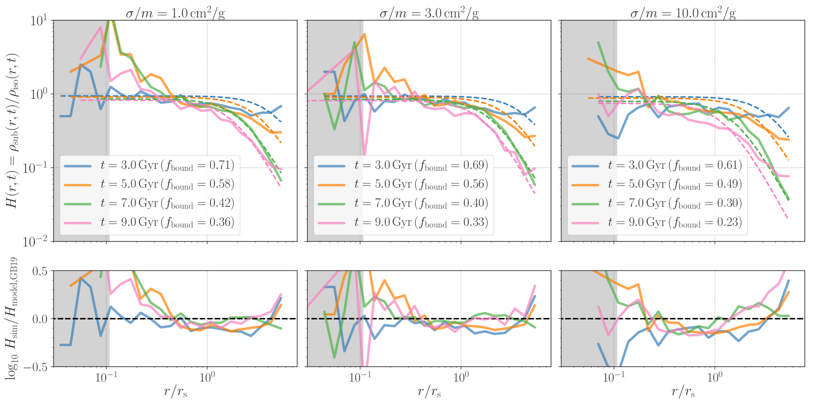
Figure 1: Structural evolution of density profiles of infalling subhaloes in SIDM models. From left to right, we show the results with the self-interacting cross section of $\sigma/m=1,3$ and $10\,\mathrm{cm}^{2}/\mathrm{g}$, respectively. For each model, the upper panel shows the transfer function of the subhalo density profile (denoted as $H(r,t)$) measured in our N-body simulations. Different coloured lines represent the results at different epochs ($t=3,5,7$, and $9\,\mathrm{Gyr}$). The dashed lines in the upper panels are model predictions in Green & van den Bosch (2019). The lower panels summarises the fractional difference between the simulation results and the model predictions. Note that numerical resolution effects would be important in the grey region in the figure. Although the model in Green & van den Bosch (2019) has been calibrated with N-body simulations with $\sigma/m=0\,\mathrm{cm}^{2}/\mathrm{g}$, it can provide a reasonable fit to the simulation results with $1\leq\sigma/m\,(\mathrm{cm}^{2}/\mathrm{g})\leq 10$ if the mass fraction of subhalo bound mass $f_{\mathrm{bound}}$ is set to the values in our N-body simulations. These results highlight that scattering processes between host- and sub-haloes are less important to determine the shape of the subhalo density profile, as long as we consider the cross section of $\sigma/m\lower 2.15277pt\hbox{$\;\buildrel<\over{\sim}\;$}10\,\mathrm{cm}^{2}/\mathrm{g}$.

3.4 For velocity-dependent cross sections

We here explain how our model can be applied for velocity-dependent cross sections $\sigma(v)/m$. Suppose that we solve the time evolution of the system with an time interval of $\Delta t$. At the $n$-th time-step $t=t_{n}$, our model follows procedures below;

1. We first determine the time evolution of density profiles for isolated host- and sub-haloes as in Subsection 3.1. For this purpose, we set effective cross sections to

   $$\left(\frac{\sigma}{m}\right)_{\mathrm{eff}} \equiv \frac{\langle\sigma v/m\rangle}{\langle v\rangle},$$ (36)

   $$\langle\sigma v/m\rangle = \int_{0}^{\infty}\mathrm{d}v\,v\,\sigma(v)/m\,f(v;v_{c}),$$ (37)

   $$\langle v\rangle = \int_{0}^{\infty}\mathrm{d}v\,v\,f(v;v_{c}),$$ (38)

   where $f(v;v_{c})$ represents the distribution function of relative velocity of particles in the host or subhalo, and $v_{c}$ determines a typical velocity scale. We define Eq. (36) with a velocity-weighted quantity because the number of particles scattered per unit time ($\propto\langle\sigma v/m\rangle$) is expected to be relevant to the evolution of SIDM density profiles. In this paper, we assume $f(v;v_{c})$ as a Maxwell-Boltzmann distribution for relative velocities;

   $$f(v;v_{c})=\frac{4v^{2}_{c}\exp(-v^{2}/v^{2}_{c})}{\sqrt{\pi}v^{3}_{c}},$$ (39)

   providing that $\langle v\rangle=v_{c}$. For a given halo/subhalo density profile at $t=t_{n-1}$, we determine the 1D velocity dispersion $\sigma_{v}(r)$ by Eq. (11) and set $v_{c}=4\sigma_{v}(r_{s})/\sqrt{\pi}$ where $r_{s}$ is the scaled radius at the initial NFW profile. We then take the corresponding SIDM density profile at $\sigma/m=(\sigma/m)_{\mathrm{eff}}$ and the moment of $t=t_{n}$ from a pre-stored table of $\rho_{\mathrm{SIDM}}$ given by Eq. (16) for $v$-independent cross sections.

2. We then solve the equation of motion of the subhalo as in Subsection 3.2. To determine the ram-pressure deceleration term of Eq. (23), we substitute $\sigma/m$ for $\sigma(|{\bf v}_{\mathrm{sub,n-1}}|)/m$, where ${\bf v}_{\mathrm{sub,n-1}}$ is the bulk velocity of the subhalo at $t=t_{n-1}$. Using the time-step of $\Delta t$, we also set the mass loss of the infalling subhalo and update the shape of the subhalo density profile as in Eq. (35). For the velocity-dependent cross section, we compute the mass loss of Eq. (32) by setting $\sigma/m=\sigma(|{\bf v}_{\mathrm{sub,n-1}}|)/m$.

3. After updating the bound mass, position, velocity, and the density profile of the subhalo, we go back to the step (i) to determine the density profiles at $t=t_{n+1}$.

4 Results

This section presents main results in our paper. Those include the structural evolution of subhalo density profiles with dark matter self-interactions, detailed comparisons with our semi-analytic model and the simulation outputs, and discussion on differences between our model and others in the literature.

4.1 Structural evolution of SIDM subhaloes

We first study density profiles of infalling SIDM subhaloes at different epochs. As the subhalo orbit is evolved, the density profile is modified by gravitational interactions as well as the self-interaction of dark matter particles in the host and subhalo.

For ease of comparison, we run N-body simulations of an isolated halo with its initial mass of $10^{9}M_{\odot}$ and concentration of $6$, but varying $\sigma/m=1,3$, and $10\,\mathrm{cm}^{2}/\mathrm{g}$. These isolated haloes are evolved by $10\,\mathrm{Gyr}$ with a snapshot interval of $0.1\,\mathrm{Gyr}$. We then characterise the structural evolution of infalling subhalo density profiles as

$$H(r,t)\equiv\frac{\rho_{\mathrm{sub}}(r,t)}{\rho_{\mathrm{iso}}(r,t)},$$ (40)

where $\rho_{\mathrm{sub}}(r,t)$ is the density profile of infalling subhaloes, and $\rho_{\mathrm{iso}}(r,t)$ represents the counterpart for isolated haloes with the same initial density profiles as the subhaloes.

Figure 1 summarises our measurements of $H(r,t)$. At each column, upper and lower panels present the results at $\sigma/m=1,3$ and $10\,\mathrm{cm}^{2}/\mathrm{g}$ from left to right. Solid lines in the upper panel show the function of $H(r,t)$ in our simulations and the colour difference indicates the difference in the epoch $t$. The coloured dashed lines in the upper panel are the prediction in Green & van den Bosch (2019) with the simulated value of the bound mass fraction $f_{\mathrm{bound}}$. The fractional difference between the simulation results and the model prediction is shown in the lower panels.

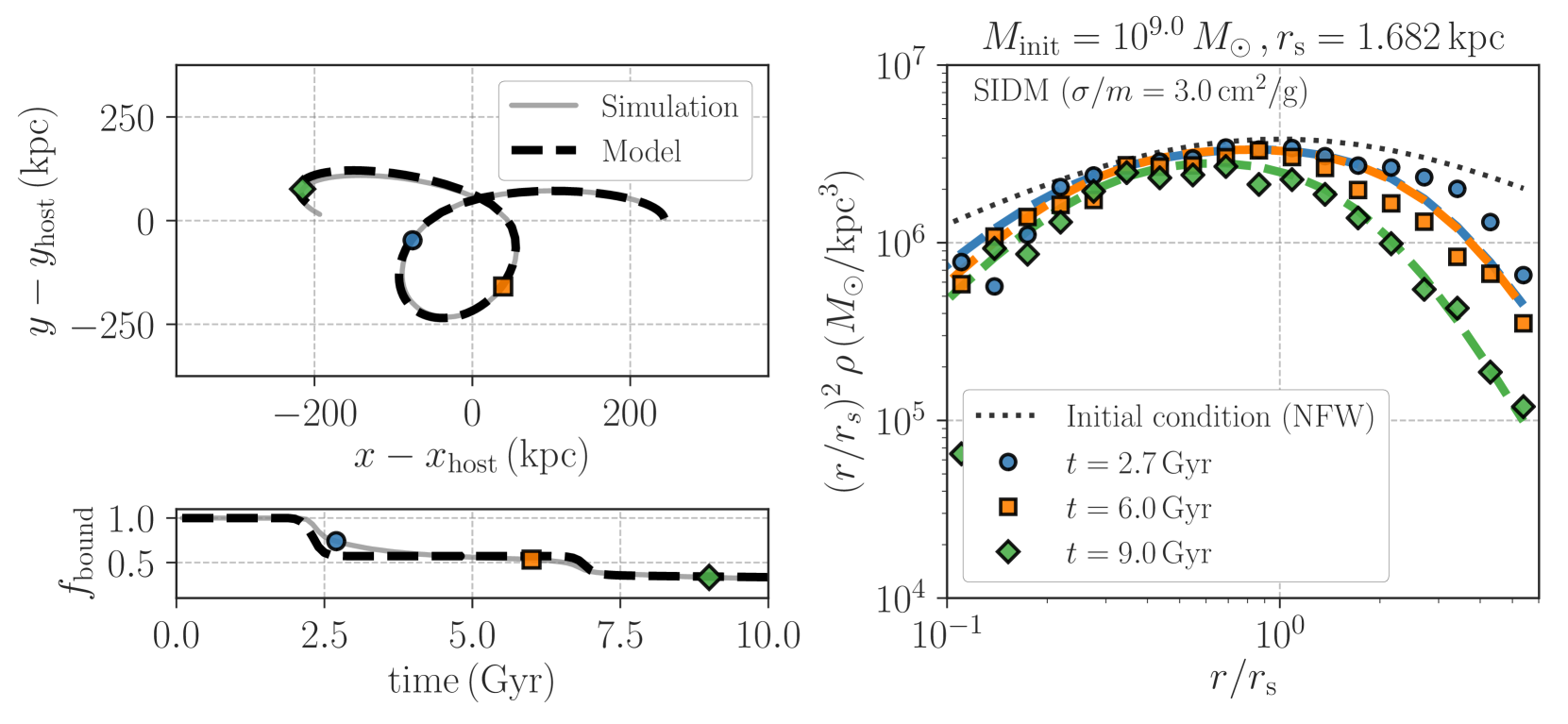
Figure 2: Comparisons with N-body simulation results and our semi-analytic model of infalling subhaloes. In this figure, we assume a velocity-independent cross section of $\sigma/m=3\,\mathrm{cm}^{2}/\mathrm{g}$. The top left panel shows the orbital evolution of the subhalo over 10 Gyr, while the bottom left presents the mass evolution. The right panel summarises the time evolution of the subhalo density profile. In the right, blue circles, orange squares, and green diamonds represent the simulation results at $t=2.7$, 6.0, and 9.0 Gyr, respectively. In each panel, dashed lines are the model predictions.

We find that the structural evolution of SIDM subhaloes can be approximated as the model in Green & van den Bosch (2019), even though the model has been calibrated with the collision-less N-body simulations. As long as the cross section is set to smaller than $\sim 10\,\mathrm{cm^{2}}/\mathrm{g}$, the ram-pressure evaporation is less important to set the shape of the subhalo density profile. We here note that a reasonable match between the simulation results and the model in Green & van den Bosch (2019) occurs only when we use the value of $f_{\mathrm{bound}}$ in the simulations. This highlights that a precise model of the mass loss is important to determine the density profile of the subhalo at outskirts across its orbit. Also, the results in Figure 1 support that our approximation of Eq. (35) would be valid if we can predict the density profile of SIDM halos in isolation. More detailed comparisons with the simulation results and Eq. (35) are presented in the next Subsection.

4.2 Comparison with simulation results and model predictions

We here summarise comparisons with our N-body simulation results and model predictions as in Section 3.

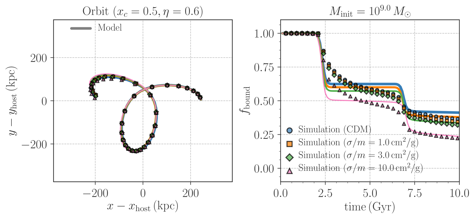
Figure 3: The orbital and mass evolution of an infalling subhalo with its initial mass of $10^{9}\,M_{\odot}$ as a function of $\sigma/m$. In this figure, $\sigma/m$ is assumed to be velocity-independent. In each panel, the blue circles, orange squares, green diamonds, and pink triangles represent the simulation results at $\sigma/m=0,1,3$, and $10\,\mathrm{cm}^{2}/\mathrm{g}$, respectively. Our model predictions are shown by different lines, providing a reasonable fit to the simulation results.

4.2.1 Varying cross sections

We first investigate the dynamical evolution of infalling subhaloes with their initial mass of $10^{9}M_{\odot}$ and a fixed subhalo orbital parameter as a function of the self-interaction cross section $\sigma/m$. For this purpose, we use the fiducial simulation runs of CDM, SIDM1, and SIDM3, and SIDM10 in Table 1.

Figure 2 summarises the simulation outputs of the infalling subhalo for the SIDM3 run ($\sigma/m=3\,\mathrm{cm}^{2}/\mathrm{g}$) as well as our model predictions. In the left panels, grey lines represent the simulation results, while the dashed lines are our model predictions. For this figure, we set a parameter for the mass loss (see Eq. 27) to ${\cal A}=0.65$. Our model provides an accurate fit to the subhalo orbit in our simulation over 10 Gyr, and the overall evolution of the subhalo mass can be captured by the simple model in Subsection 3.3. In the right panel, we compare the subhalo density profile at different epochs. The simulation results are shown by coloured symbols, and the dashed lines show the model predictions. The figure demonstrates that the structural evolution of the subhalo density profile can be explained by our phenomenological model of Eq. (35). The time evolution at $r\lower 2.15277pt\hbox{$\;\buildrel<\over{\sim}\;$}r_{s}$ can be well determined by the gravothermal fluid model with a correction (see Eq. 16), while the density at outskirts ($r\lower 2.15277pt\hbox{$\;\buildrel>\over{\sim}\;$}r_{s}$) is suppressed mostly by tidal stripping processes.

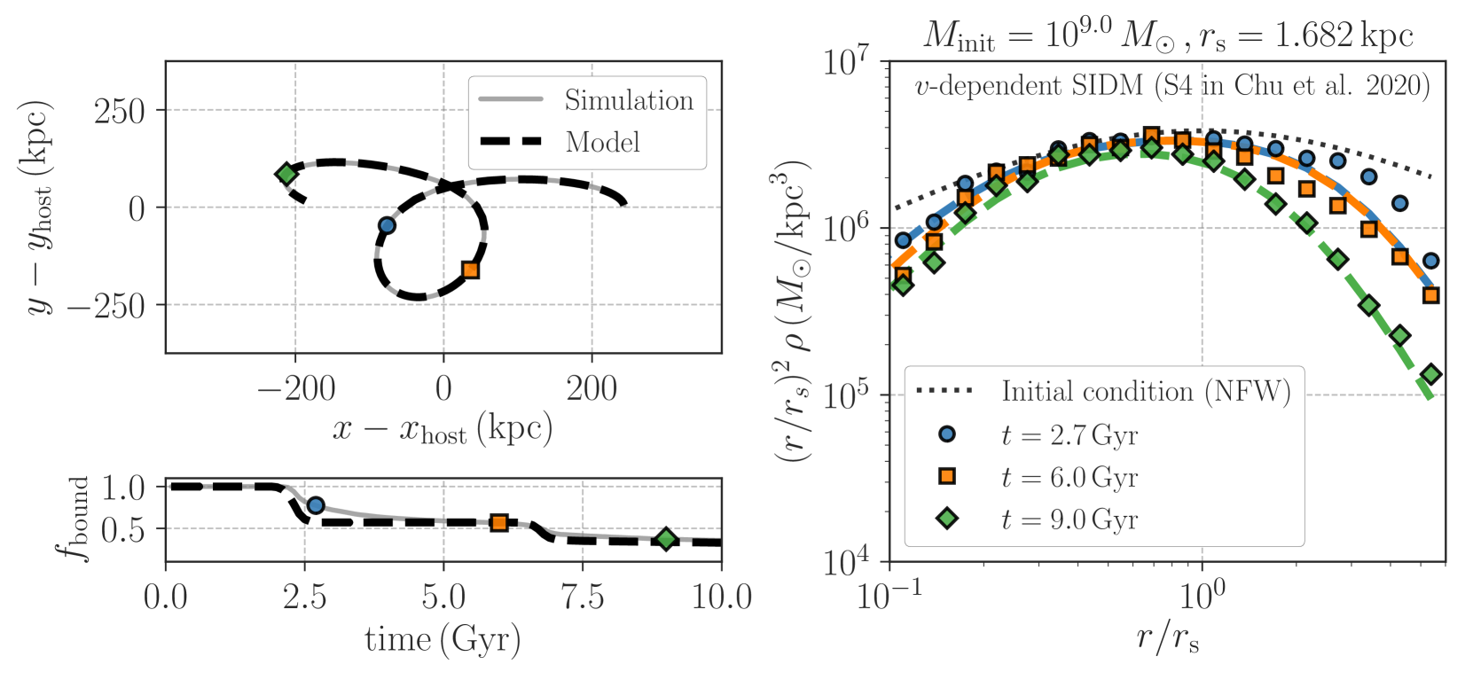
Figure 4: Similar to Figure 2, but we consider a velocity-dependent cross section given by Eq (10).

Figure 3 shows how the dynamical evolution of the subhalo can depend on the cross section $\sigma/m$. The orbital evolution of the subhalo with different $\sigma/m$ are summarised in the left, while the right shows the evolution of the subhalo mass over 10 Gyr. In each panel, solid lines represent our model predictions, providing a reasonable fit to the simulation results for various cross sections. We find that the model works when the parameter $\cal A$ is set to $0.55$, $0.60$, $0.65$ and $0.75$ for the simulations with $\sigma/m=0,1,3$, and $10\,\mathrm{cm}^{2}/\mathrm{g}$, respectively. This marginal $\sigma/m$-dependence of the model parameter $\cal A$ can be important in practice, especially when one would constrain the SIDM by using observations of MW satellites. We also note that the subhalo mass is more suppressed as $\sigma/m$ becomes larger in our simulations and this looks compatible with recent studies (e.g. Sameie et al., 2020).

We then examine the velocity-dependent model of $\sigma/m$ as in Eq. (10) by using the vSIDM run (see Table 1). Figure 4 summarises the comparison of the simulation results with our semi-analytic model. Note that we set ${\cal A}=0.65$ in Figure 4. The figure highlights that our treatment in Subsection 3.4 can explain the simulation results with an appropriate choice of ${\cal A}$.

4.2.2 Varying subhalo orbits

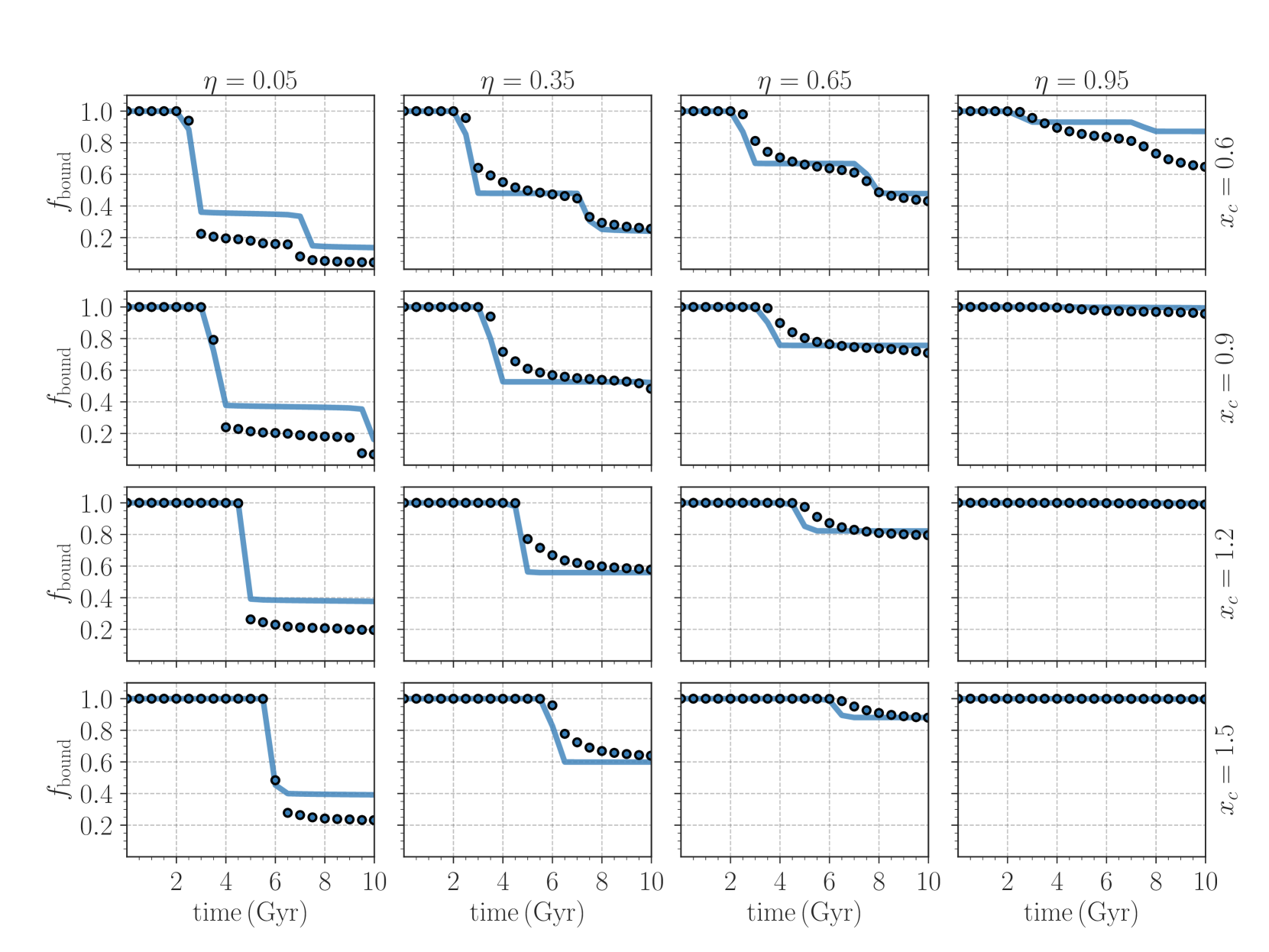
Figure 5: The mass evolution of infalling subhaloes at various orbits for the SIDM model with the velocity-independent cross section of $1\,\mathrm{cm}^{2}/\mathrm{g}$. In each panel, the blue circles show the simulation results, while the line presents our model prediction. The subhalo orbits are characterised by two parameters of $x_{c}$ and $\eta$. The results with $\eta=0.05,0.35,0.65$, and $0.95$ are shown from left to right, while we increase $x_{c}$ as $x_{c}=0.6,0.9,1.2$, and $1.5$ from top to bottom. Note that larger $x_{c}$ corresponds to longer orbital period, and smaller $\eta$ provides more radial orbits (see Subsection 2.1 for details).

We next study the impact of subhalo orbits on the subhalo mass loss in SIDM models. We examine 16 different sets of our orbital parameters $(x_{c},\eta)$ as in Table 1 assuming the velocity-independent cross section of $\sigma/m=1\,\mathrm{cm}^{2}/\mathrm{g}$.

Figure 5 summarises the time evolution of infalling subhalo masses as a function of $(x_{c},\eta)$. The blue circles in the figure represent the simulation results, while the solid lines show our model predictions. We assume ${\cal A}=0.60$ for every model prediction in the figure. We find that our model can provide a reasonable fit to the simulation results with $\eta\lower 2.15277pt\hbox{$\;\buildrel>\over{\sim}\;$}0.35$ and a range of $0.6\leq x_{c}\leq 1.5$, but a sizeable difference between the simulation results and our model can be found at an extreme value of $\eta\simeq 0.05$. Note that orbits with $\eta\lower 2.15277pt\hbox{$\;\buildrel<\over{\sim}\;$}0.2$ rarely happens in cosmological simulations of collision-less dark matter (e.g. Jiang et al., 2015). Even for the orbits at $\eta=0.05$, our model can explain overall trends in the time evolution of the subhalo mass with a level of $20-30\%$.

4.2.3 Model precision of subhalo density profiles

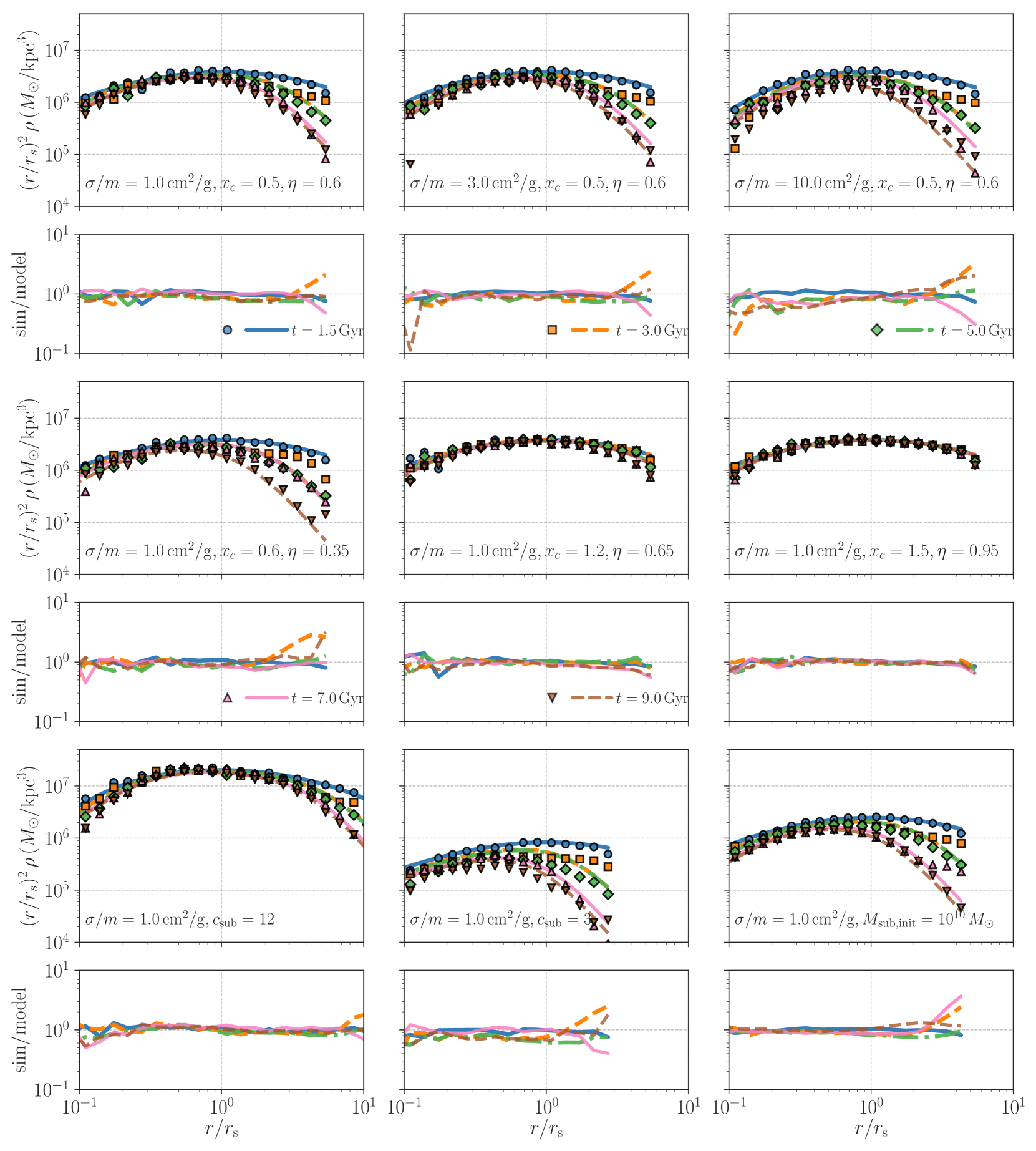
Figure 6: Precision of the subhalo density profile by our semi-analytic model. At the first, third, and fifth rows, coloured symbols show the density profiles in our N-body simulations at different epochs of $t=1.5,3,5,7$ and 9 Gyr, while the coloured lines are our model predictions. Each panel at the second, fourth, and six rows show the ratio between the density profile in our N-body simulations and our model counterparts for the ease of comparison. At the first and second rows, we show the results at a fixed subhalo orbit, but increase the cross section as $\sigma/m=1,3$, and $10\,\mathrm{cm}^{2}/\mathrm{g}$ from left to right. At the third and fourth rows, we fix the cross section to $\sigma/m=1\,\mathrm{cm}^{2}/\mathrm{g}$, but change the subhalo orbits. At the fifth and sixth rows, we examine different density profiles of subhaloes at $t=0$ in the SIDM model with $\sigma/m=1\,\mathrm{cm}^{2}/\mathrm{g}$.

We then investigate the subhalo density profiles at various initial conditions as well as examine the dependence on the self-interaction cross section $\sigma/m$. Figure 6 compares the subhalo density profiles in our N-body simulations with the model counterparts. In this figure, the first, third and fifth rows summarise the subhalo density profiles in various simulation runs. At those rows, different coloured symbols represent the subhalo density profiles in the simulation at different epochs of $t=1.5,3,5,7$ and $9\,\mathrm{Gyr}$, while the coloured lines are the counterparts by our model prediction. At the second, fourth, and sixth rows, individual panels show the ratio between the simulation results and our model predictions for comparison.

At the first and second rows, we show the results as varying $\sigma/m$ for a fixed initial condition of the subhalo. We observe that our model can reproduce the subhalo density profiles in the simulations with a level of $\sim 0.1$ dex in a range of $r/r_{s}\lower 2.15277pt\hbox{$\;\buildrel>\over{\sim}\;$}1$ when varied the cross section $\sigma/m$. The model precision becomes worse as we increase $\sigma/m$, implying that effects of gravothermal instability may be required to be revised for a better model.

Three panels at the third and fourth rows summarise the comparisons at different orbital parameters $(x_{c},\eta)$ for the SIDM model with $\sigma/m=1\,\mathrm{cm}^{2}/\mathrm{g}$. As long as the orbital parameter is set to be $\eta\lower 2.15277pt\hbox{$\;\buildrel>\over{\sim}\;$}0.35$, our model can provide an accurate fit to the simulation results. Note that a small value of $\eta$ corresponds to a highly elongated orbit around the host. When setting an extreme condition of $\eta=0.05$, we observed that our model precision gets worse (but the model has a 0.5 dex level precision). For tidal effects, our model partly relies on the assumption of the subhalo on a circular orbit (Eq. 30). Hence the model would tend to be invalid for more radial orbits.

In the panels at the fifth and sixth rows, we can see the effect of initial conditions of subhaloes for the SIDM model with $\sigma/m=1\,\mathrm{cm}^{2}/\mathrm{g}$. The left panel at the fifth row shows the comparisons when we assume an initial subhalo density profile with a higher concentration, while the middle bottom panel presents the results with the subhalo with a lower concentration at $t=0$. We find that our model can reproduce the simulation results with a level of $\sim 0.2$ dex for a wide range of the subhalo concentration at their initial density. The model precision gets worse for the lower-concentration subhalo, indicating that a more detailed calibration of the gravothermal fluid model (see Eq. 16) and the tidal stripping model (see Eq. 35) are beneficial. The right panel at the fifth row in the figure summarises the comparisons when we increase the subhalo mass at its initial state as $M_{\mathrm{sub}}=10^{10}\,M_{\odot}$. We do not observe any systematic trends in the difference between the simulation results and our model predictions even if we increase the initial subhalo mass.

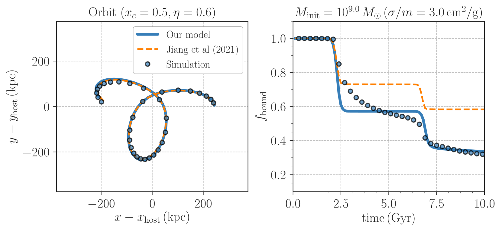
Figure 7: Similar to Figure 3, but we include the model prediction in Jiang et al. (2021a). In this figure, we assume a velocity-independent cross section of $\sigma/m=3\,\mathrm{cm}^{2}/\mathrm{g}$. The blue circles show our simulation results, the solid lines are our model predictions, and the orange dashed lines represent the model in Jiang et al. (2021a).

4.3 Comparison with previous studies

In the aforementioned sections, we introduced a semi-analytic model of infalling subhaloes and made detailed comparisons with ideal N-body simulation results and the model predictions. We here discuss differences among our model and others in the literature.

4.3.1 Time evolution of density profiles of single SIDM haloes

Our model assumes a gravothermal fluid model based on the calibration of the thermal conductivity $\kappa$ in Eq. (13) in Koda & Shapiro (2011), whereas we further include a correction based on our N-body simulations of isolated SIDM haloes as in Eq. (16). Previous studies have reported different models of $\kappa$ for isolated and cosmological N-body simulations (e.g. Balberg et al., 2002; Koda & Shapiro, 2011; Essig et al., 2019; Nishikawa et al., 2020). Also, the hydrostatic equilibrium (Eq. 11) is not always valid in SIDM haloes at small cross sections (e.g. Nishikawa et al., 2020). Hence, a correction of the gravothermal fluid model would be needed for a precise modelling of time evolution of SIDM density profiles. Nevertheless, it would be worth noting that we correct the gravothermal fluid model with a level of 10-50% over 10 Gyr. From a qualitative point of view, the fluid model in Koda & Shapiro (2011) provides a fit to our N-body simulation results.

For another approach, Robertson et al. (2021) introduced a mapping method from a given NFW profile to an isothermal density profile based on Jeans equations, referred to as isothermal Jeans modelling. In the isothermal Jeans modelling, one assumes that a SIDM halo follows an isothermal density profile at the radius smaller than $r_{c}$, while the NFW profile remains unchanged at outer radii. The isothermal Jeans modelling is found to be valid when one predicts the density profile of a SIDM halo at a given epoch, but a proper choice of $r_{c}$ is required to explain simulation results on a case-by-case basis. Hence, the isothermal Jeans modelling is less relevant to predicting the time evolution of the SIDM density profile.

4.3.2 Evolution of infalling subhaloes

Our model assumes that the motion of infalling SIDM subhaloes is governed by Eq. (20) as same as in Jiang et al. (2021a). The model of Jiang et al. (2021a), referred to as J21 model, assumes that (i) an isolated SIDM halo follows a cored profile with a characteristic core radius where every particle is expected to have interacted once within a time, (ii) a parameter of the mass loss in Eq. (27) is fixed to ${\cal A}=0.55$ as expected in the collision-less dark matter (Green et al., 2021), and (iii) the mass loss by tidal stripping effects (Eq. 27) truncates the subhalo boundary radius and the mass loss by self-interactions (Eq. 32) decreases the amplitude in the subhalo density. We also refer the readers to a brief description of the J21 model in Appendix E.

Figure 7 summarises the comparison with the J21 model and ours for the SIDM with the cross section of $\sigma/m=3\,\mathrm{cm}^{2}/\mathrm{g}$. We find that the difference in the subhalo orbit is very small. On the time evolution of the subhalo mass, an appropriate choice of the parameter ${\cal A}$ is needed to provide a better fit to our simulation results. Note that Jiang et al. (2021a) assumes a static NFW gravitational potential for the host halo in their analysis. Hence, the orbital evolution of infalling subhaloes in Jiang et al. (2021a) may be less affected by choices of the model, whereas the J21 model would have a $50\%$-level uncertainty in predicting the time evolution of the subhalo mass over $\sim 10\,\mathrm{Gyr}$.

Recently, Correa (2021) has developed a semi-analytic model of infalling subhaloes in a static host based on a gravothermal fluid model and derived an interesting constraint of SIDM models with observations of MW dwarf spheroidal galaxies. The model in Correa (2021) incorporated the gravothermal fluid model with the tidal evolution of subhaloes (van den Bosch et al., 2018; Green & van den Bosch, 2019), accounting for the gravothermal collapse effects accelerated by the tidal stripping (Nishikawa et al., 2020; Sameie et al., 2020). However, the model computes the mass loss rate assuming a circular subhalo orbit and does not include the mass loss by the self-scattering-induced evaporation. This simplification can affect the subhalo mass at each moment. Because the gravothermal instability depends on how the subhalo mass density is tidally stripped, further developments would be interesting for a precise modelling of the gravothermal collapse effects in infalling subhaloes. Note that our model ignores the gravothermal instability induced by tidal stripping effects, while it can solve the orbital and structural evolution of subhaloes in a self-consistent way.

5 Limitations

Before concluding, we summarise the major limitations in our semi-analytic model of infalling subhaloes in a MW-sized host halo. The following issues will be addressed in future studies.

5.1 Baryonic effects

In this paper, we do not consider any baryonic effects. Baryons can affect our semi-analytic model in various ways.

The presence of stellar and gas components is common in most of real galaxies. The baryons at the galaxy centre can deepen the gravitational potential compared to dark-matter-only predictions. This allows an effective temperature of SIDM particles to have a flat or negative gradient in the radius, leading to decrease the size of SIDM core as well as increase the central SIDM density in baryon-dominated galaxies (Kaplinghat et al., 2014; Kamada et al., 2017b). These back-reaction effects between baryons and SIDM have been investigated in isolated N-body simulations (Sameie et al., 2018) and cosmological zoom-in simulations (Vogelsberger et al., 2014; Fitts et al., 2019; Robles et al., 2019; Sameie et al., 2021). Interestingly, the simulations in Sameie et al. (2018) showed that the SIDM core in a MW-sized halo can expand at early phases and contract later. This time variation can be important to predict orbits of infalling subhaloes in a realistic MW-sized galaxy.

In addition, the presence of stellar disc at the host centres can severely affect the mass loss of infalling subhaloes. D’Onghia et al. (2010) showed that subhaloes in the inner regions of the halo are efficiently destroyed in the presence of time-evolving stellar disc components, while Garrison-Kimmel et al. (2017) found that this suppression in the subhalo abundance can be explained by adding an embedded central disc potential to dark-matter-only simulations. Isolated N-body simulations also play important roles in studying the depletion of subhaloes in details (e.g Peñarrubia et al., 2010; Errani et al., 2017). Recently, Green et al. (2022) have explored the impact of a galactic disc potential on the subhalo populations in MW-like haloes with their semi-analytic modelling. We expect that our semi-analytic model can be useful to investigate the effects of stellar disc components in the SIDM model by adding a stellar disc potential in the equation of motion (Eq. 20).

5.2 Gravothermal collapse

The gravothermal instability induces dynamical collapse of the SIDM core. This effect can be partly taken into account in our semi-analytic model with the gravothermal fluid model (see Subsection 3.1). Note that the gravothermal fluid model of isolated SIDM haloes predicts the core collapse over time, but it rarely happens within a Hubble time (e.g. Balberg et al., 2002). Our model still assumes that the gravothermal collapse occurs regardless of the tidal stripping effects, but this is not the case for some specific conditions (Nishikawa et al., 2020; Sameie et al., 2020). Nishikawa et al. (2020) found that the core collapse in the SIDM density can realise within a Hubble time for $\sigma/m\lower 2.15277pt\hbox{$\;\buildrel<\over{\sim}\;$}10\,\mathrm{cm}^{2}/\mathrm{g}$ if the initial subhalo density is significantly truncated, while Sameie et al. (2020) showed that the evolution of the SIDM core is sensitive to the concentration in the initial subhalo density. Motivated by those findings, Correa (2021) developed a gravothermal fluid model of tidally stripped subhaloes with focus on a large self-interacting cross section of $20-150\,\mathrm{cm}^{2}/\mathrm{g}$. A calibration of the gravothermal fluid model in Correa (2021) with N-body simulations would be an interesting direction of future studies.

5.3 Comparisons with cosmological simulations

Our semi-analytic model has been calibrated with isolated N-body simulations. This indicates that our results may be affected by cosmological environments at the outermost radii. A lumpy and continuous mass accretion in an expanding universe can heat SIDM haloes, slowing the gravothermal core collapse. Detailed comparisons with our gravothermal fluid model of Eq. (16) with cosmological SIDM N-body simulations (e.g. Rocha et al., 2013; Elbert et al., 2015) can reveal how important environmental effects are in predicting time evolution of the SIDM density profiles.

The evolution of infalling subhaloes can be affected by other floating subhaloes in the host. The subhaloes should gravitationally interact with each other, and induce perturbations in the host gravitational potential. These complex effects might affect the orbital and structural evolution of infalling subhaloes. To examine these, it would be worth comparing our semi-analytic model with zoom-in simulation results of MW-sized cosmological haloes (e.g. Ebisu et al., 2022).

6 Conclusions and discussions

In this paper, we have studied the evolution of a $10^{9}\,M_{\odot}$ subhalo infalling onto a MW-sized host halo in the presence of self-interactions among dark matter particles. We have performed a set of dark-matter-only N-body simulations of halo-subhalo minor mergers by varying self-interacting cross sections $\sigma/m$, subhalo orbits, and initial conditions of subhalo density profiles. For comparisons, we developed a semi-analytic model of infalling subhaloes in a given host halo by combining a gravothermal fluid model with subhalo mass losses due to tidal stripping and ram-pressure-induced effects. We then made detailed comparisons with our simulation results and the semi-analytic model, allowing to improve physical understanding of self-interacting dark matter (SIDM) substructures. Although our study imposes several assumptions, we gained meaningful insights as follows:

1. In our N-body simulations for a range of $\sigma/m\lower 2.15277pt\hbox{$\;\buildrel<\over{\sim}\;$}30\,\mathrm{cm}^{2}/\mathrm{g}$, the fluid model with the thermal conductivity calibrated in Koda & Shapiro (2011) can qualitatively explain the time evolution of the SIDM core in an isolated halo whose initial density follows a NFW profile, but we also observe systematic differences between the simulation results and the fluid model over 10 Gyr. We provided a simple correction of the model as in Eq. (16). Our corrected gravothermal fluid model allows to predict the time evolution of SIDM density profiles over 10 Gyr with a $10\%$-level precision.

2. The structural evolution of infalling subhaloes can be explained by the prediction for collision-less dark matter as proposed in Green & van den Bosch (2019), even if we include the self-interaction of dark matter particles. The evaporation due to self-interacting ram pressure can not alter the SIDM density profile in isolation as long as the cross section is smaller than $\sigma/m\lower 2.15277pt\hbox{$\;\buildrel<\over{\sim}\;$}10\,\mathrm{cm}^{2}/\mathrm{g}$. The tidal stripping effects play a central role in the change in the density profile of the SIDM subhalo across its orbit (Subsection 4.1). When the initial subhalo density is set to be consistent with the $\Lambda$CDM prediction at $z\sim 2$, the SIDM subhaloes do not undergo the gravothermal collapse over 10 Gyr in our simulations.

3. The orbit of SIDM subhaloes can be precisely predicted by a simple framework based on point-mass approximation incorporated with the dynamical friction (Chandrasekhar, 1943) and the ram-pressure-induced deceleration (Kummer et al., 2018) (Subsection 3.2).

4. The time evolution of SIDM subhalo masses can be also explained by a common method accounting for the mass loss due to tidal stripping and ram-pressure effects (Subsection 3.3). Our N-body simulations need an effective mass loss rate of the tidal stripping (Eq. 27) to depend on the self-interacting cross section $\sigma/m$, that is a new systematic effect in the prediction of SIDM subhaloes.

5. Our semi-analytic model can provide a reasonable fit to the simulation results for various cross sections (including a velocity-dependent scenario as in Eq. 10), subhalo orbits, and initial subhalo density profiles. A typical uncertainty in the model prediction is 0.1-0.2 dex for the SIDM subhalo density profiles over 10 Gyr in a range of $\sigma/m\lower 2.15277pt\hbox{$\;\buildrel<\over{\sim}\;$}10\,\mathrm{cm}^{2}/\mathrm{g}$.

Our semi-analytic model provides a simple, efficient, and physically-intuitive prediction of SIDM subhaloes, but it has to be revised in various aspects for applications to real data sets. The model should include more realistic effects, such as baryonic effects in a MW-sized host halo, the gravothermal instability induced by tidal stripping effects, cosmological mass accretion around the host halo, and gravitational interaction among subhaloes in the host (see Section 5 for details). We expect the model to be improved on a step-by-step basis with a use of cosmological N-body simulations as well as isolated N-body simulations including baryonic components in the host gravitational potential. This is along the line of our ongoing study.

Data Availability

The data underlying this article will be shared on reasonable request to the corresponding author.

Appendix A Convergence tests for N-body simulations

We here summarise convergence tests of our N-body simulations for halo-subhalo mergers. In this Appendix, we work on the same parameter sets as “SIDM1” in Table 1. We run three different N-body simulations with the particle mass of $m_{\mathrm{part}}$ being $10^{4}$, $10^{5}$ and $10^{6}\,M_{\odot}$, respectively. In each simulation, we set the gravitational softening length as in Eq (9). Note that the host halo (subhalo at $t=0$) can be resolved with $10^{8}(10^{5})$, $10^{7}(10^{4})$, and $10^{6}(10^{3})$ when we set $m_{\mathrm{part}}=10^{4}$, $10^{5}$ and $10^{6}M_{\odot}$.

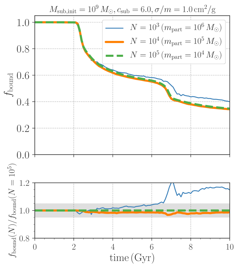
Figure 8: Convergence tests for evolution of subhalo bound mass. The top panel shows the fraction of subhalo bound mass (normalised to unity at $t=0$) when we vary the particle resolution in our simulations. The bottom panel represents the fractional difference among the simulation results. The grey shaded region in the bottom shows a $\pm 5\%$ difference. In each panel, the blue thin, orange thick, green dashed lines stand for the simulation results with $m_{\mathrm{part}}=10^{6}$, $10^{5}$ and $10^{4}\,M_{\odot}$, respectively. This figure highlights that our fiducial run with $m_{\mathrm{part}}=10^{5}\,M_{\odot}$ shows a converged result within a few percents.

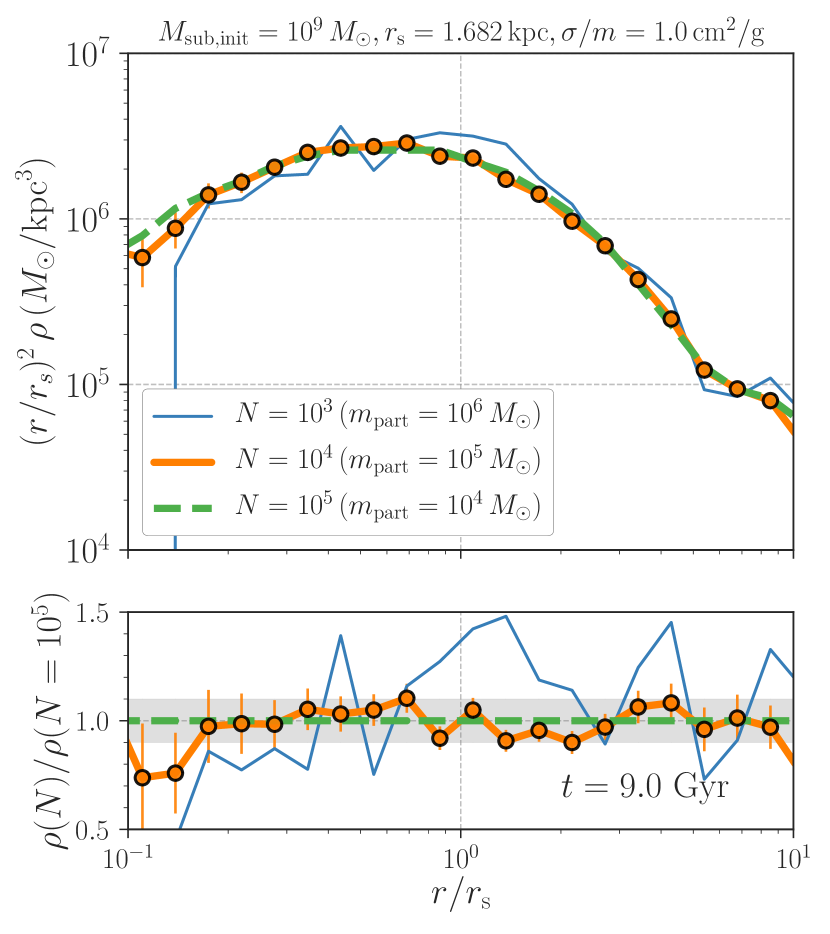
Figure 9: Convergence tests for subhalo density profiles. Similar legends are applied as in Figure 8. The top panel shows the subhalo density profiles evolved by 9 Gyr when the resolution is varied, while the bottom represents the fractional difference. The grey region in the bottom panel highlights a $\pm 10\%$ difference.

Figures 8 and 9 summarise the convergence tests in our N-body simulations. We found that our fiducial set up with $m_{\mathrm{part}}=10^{5}\,M_{\odot}$ can make the subhalo mass evolution converged within a $2-3\%$ level, while the subhalo density profile at $r/r_{s}\lower 2.15277pt\hbox{$\;\buildrel>\over{\sim}\;$}0.2$ in our simulations looks converged with a $10\%$-level precision. We caution that the inner subhalo profile may suffer from some numerical resolution effects in our simulation sets.

Appendix B A test of SIDM implementation

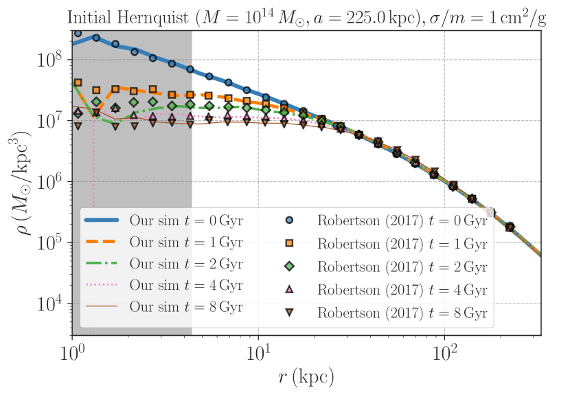
Figure 10: The halo core formation and size evolution for a Hernquist halo with $M=10^{14}\,M_{\odot}$ and the scaled radius $a=225\,\mathrm{kpc}$. In this figure, we consider the SIDM model with $\sigma/m=1\,\mathrm{cm}^{2}/\mathrm{g}$. The points show the result reported in Robertson (2017). The different lines represent our simulation results, demonstrating that our SIDM implementation provides a consistent time evolution of SIDM cores. The gray region highlights scales shorter than the gravitational softening length of $4.4\,\mathrm{kpc}$.

As a test, we consider an isolated halo following a Hernquist profile at its initial state. The Hernquist profile is expressed as

$$\rho(r)=\frac{M}{2\pi}\frac{a}{r(r+a)^{3}},$$ (41)

where $a$ is the scaled radius. For the initial Hernquist profile, we adopt the same parameters as in Robertson (2017). To be specific, we set the mass parameter of $10^{14}\,M_{\odot}$ and the scaled radius of $225\,\mathrm{kpc}$. We ran the simulation with $128^{3}$ N-body particles, the gravitational softening length of $4.4\,\mathrm{kpc}$, and the cross section of $\sigma/m=1\,\mathrm{cm}^{2}/\mathrm{g}$. Note that those simulation parameters are also same as in Robertson (2017). For comparison, we extract the data points of SIDM density profiles from Figure 4.9 in Robertson (2017) by using this website. Figure 10 summarises the comparison of the halo core evolution for the Hernquist halo in our simulation with the results in Robertson (2017). We confirm that our SIDM implementation provides a good fit to the results in the literature.

Appendix C Calibration of gravothermal fluid model for an isolated halo

In this Appendix, we describe our calibration of the gravothermal fluid model. For the calibration, we perform N-body simulations of an isolated halo with its initial density profile following a NFW profile as varying the self-interacting cross section $\sigma/m$. In these isolated simulations, we set the halo mass and the scaled radius at $t=0$ to be $10^{12}\,M_{\odot}$ and $r_{s}=21.18\,\mathrm{kpc}$. We examine five cross sections of $\sigma/m=0.3,1,3,10$ and $30\,\mathrm{cm}^{2}/\mathrm{g}$ and evolve the halo by 10 Gyr in our simulations. The simulation outputs are stored with a time interval of $0.1\,\mathrm{Gyr}$, producing 100 snapshots for a given SIDM model. We refer the readers to Subsection 2.1 about how to prepare an isolated NFW halo.

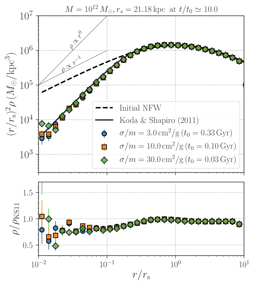
Figure 11: SIDM density profiles as a function of the cross section $\sigma/m$. In the upper panel, the solid line shows the gravothermal fluid model with the heat conductivity calibrated in Koda & Shapiro (2011), while different coloured symbols represent our N-body simulation results for an isolated halo with its mass of $10^{12}\,M_{\odot}$. We show the simulation results at a dimensionless time $t/t_{0}=10$, where $t_{0}$ is a characteristic relaxation time scale given in Eq. (19). Because the time scale $t_{0}$ depends on $\sigma/m$, each symbol represents the density profile at different epoch; The blue circle shows the density profile at $t\simeq 3.3\,\mathrm{Gyr}$ for the SIDM with $\sigma/m=3\,\mathrm{cm}^{2}/\mathrm{g}$, while the orange square and green diamond show the counterparts at $t\simeq 1.0\,\mathrm{Gyr}$ and $t\simeq 0.3\,\mathrm{Gyr}$ for $\sigma/m=10\,\mathrm{cm}^{2}/\mathrm{g}$ and $30\,\mathrm{cm}^{2}/\mathrm{g}$, respectively. Note that the upper panel shows the quantity of $\sim r^{2}\rho$. For ease of comparisons, we also show the initial NFW profile by the dashed line in the top panel. The bottom panel shows the fractional difference between the gravothermal fluid model and the simulation results at $t/t_{0}=3$, highlighting that a universal correction can be applied to the gravothermal fluid prediction for various $\sigma/m$.

Figure 11 summarises the comparison of the SIDM density profile between the simulation results and the gravothermal fluid model in Koda & Shapiro (2011). In the figure, we show the density profiles at a dimensionless epoch $t/t_{0}=10$, where $t_{0}$ is given by Eq. (19). Once considering evolution with respect to dimensionless epochs $t/t_{0}$, we find that the gravothermal fluid model predicts almost an identical density profile at a given $t/t_{0}$ regardless of the exact value of $\sigma/m$. The gravothermal fluid prediction is shown by the solid line in the top panel of figure 11, while different coloured symbols represent our simulation results at $t/t_{0}=10$. Although the simulation results exhibit a $O(10)\%$ difference from the gravothermal fluid model at $r/r_{s}\simeq 0.1$, the difference is found to be almost independent on $\sigma/m$ if comparing the density profiles at the same dimensionless epoch $t/t_{0}$. This finding motivates us to develop a correction function of the gravothermal fluid model below;

$$\rho_{\mathrm{SIDM}}(r,t,\sigma/m)=\rho_{\mathrm{gt}}(r,t,\sigma/m)\,{\cal C}(r/r_{s},t/t_{0}),$$ (42)

where ${\cal C}$ represents the correction function which we would like to find. After some trials, we find that our simulation results can be well explained by a two-parameter function below;

$${\cal C}(x,\tilde{t})=\frac{x^{\beta}+(1/2)^{\beta}}{(x+\gamma)^{\beta}},$$ (43)

where $x=r/(0.1r_{s})$ and we assume that $\beta$ and $\gamma$ depend on $\tilde{t}=t/t_{0}$.

Using the density profile of the simulated halo at a given snapshot and cross section of $\sigma/m$, we find the best-fit parameters of $\beta$ and $\gamma$ by minimising the chi-square value of

$$\chi^{2}=\sum_{i}\left[\rho_{\mathrm{sim}}(r_{i},t,\sigma/m)-\rho_{\mathrm{SIDM}}(r_{i},t,\sigma/m)\right]^{2},$$ (44)

where $\rho_{\mathrm{sim}}$ represents the density profile of the simulated halo and $r_{i}$ is the $i$-th bin in the halo-centric radius. For this chi-square analysis, we perform a logarithmic binning in $r/r_{s}$ with the number of bins being 35 in a range of $0.01<r/r_{s}<30$ when computing the spherical density profile of the simulated halo. After finding the best-fit parameters for a given set of snapshot time $t$ and cross section $\sigma/m$, we derive the $t/t_{0}$-dependence as in Eqs. (17) and (18). Figure 12 summarises our calibration, demonstrating that the model of Eq. (16) can provide a good fit to the simulation results for a wide range of $\sigma/m$ and $t$. We confirm that our calibrated model has a $10\%$-level precision in the range of $t/t_{0}\lower 2.15277pt\hbox{$\;\buildrel<\over{\sim}\;$}100$. It would be worth noting that our model has been calibrated for a specific initial condition. Hence, our model can not be applied to general cases, but it would provide a reasonable fit to the SIDM density profile as long as its initial density follows a NFW profile. A caveat is that our calibration may depend on a choice of boundary radius in an isolated SIDM halo as discussed in Koda & Shapiro (2011). Note that the model in Koda & Shapiro (2011) has been calibrated with simulation results assuming the halo boundary radius is set to 100 times as large as the NFW scaled radius, while we adopted a more realistic situation (i.e. the halo concentration of 10). We leave it to investigate possible effects of the halo boundary radii in SIDM simulations for future studies.

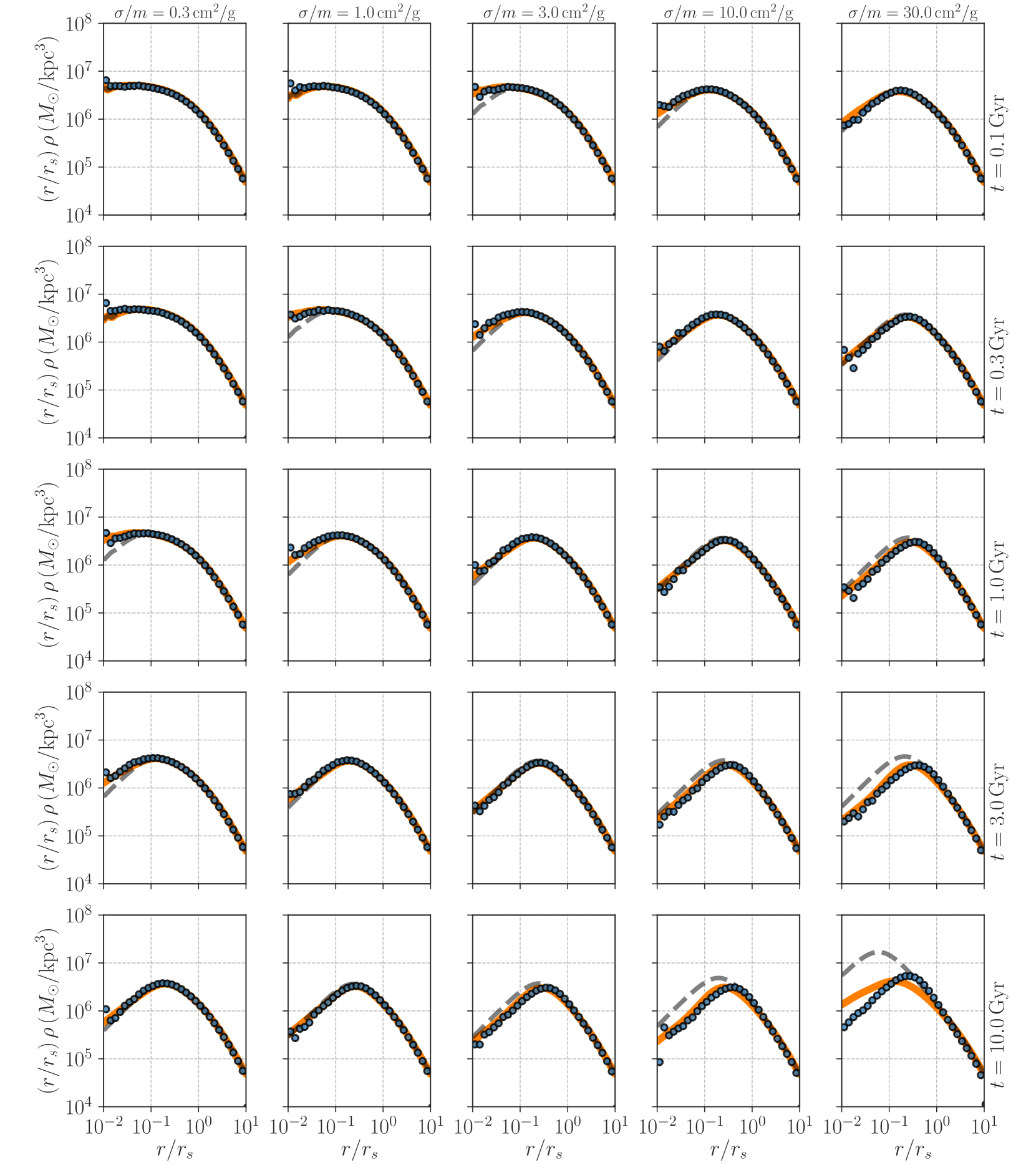
Figure 12: Tests of our calibrated gravothermal fluid model (Eq. 16) against the N-body simulations of an isolated halo. In each panel, the blue circles show the simulation results, while the grey dashed and orange solid lines represent the model in Koda & Shapiro (2011) and our calibrated model, respectively. From left to right (top to bottom), we show the comparisons as increasing $\sigma/m$ (epoch $t$).

Appendix D A fitting formula of the transfer function for tidally truncated density profiles

In this appendix, we provide a fitting formula of the transfer function developed in Green & van den Bosch (2019). In the context of tidal evolution of collision-less dark matter subhaloes, the transfer function is commonly defined as

$$H(r,t)=\frac{\rho(r,t)}{\rho(r,t=0)},$$ (45)

where $H$ is the transfer function, $r$ is the radius from the centre of the subhalo, and $\rho(r,t)$ is the subhalo density profile at an epoch of $t$. Using a set of collision-less N-body simulations of minor mergers, Green & van den Bosch (2019) found that $H$ can be well approximated as the form below;

$$H(r,t)=\frac{f_{\mathrm{te}}}{1+\left(\tilde{r}\left[\frac{\tilde{r}_{\mathrm{sub,vir}}-\tilde{r}_{\mathrm{te}}}{\tilde{r}_{\mathrm{sub,vir}}\tilde{r}_{\mathrm{te}}}\right]\right)^{\delta}},$$ (46)

where $\tilde{r}=r/r_{\mathrm{s,init}}$ such that all radii in Eq. (46) are normalized to the initial NFW scale radius of the subhalo $r_{\mathrm{s,init}}$.

Eq. (46) contains three model parameters and those depend on the initial subhalo concentration $c_{\mathrm{sub}}$ and the bound mass fraction of the subhalo at the epoch $t$ (denoted as $f_{\mathrm{bound}}$). Throughout this paper, we adopt

$$f_{\mathrm{te}} = f^{a_{1}(c_{\mathrm{sub,10}})^{a_{2}}}_{\mathrm{b}}\,c^{a_{3}(1-f_{\mathrm{bound}})^{a_{4}}}_{\mathrm{sub}},$$ (47)

$$\tilde{r}_{\mathrm{te}} = \tilde{r}_{\mathrm{sub,vir}}\,f^{b_{1}(c_{\mathrm{sub,10}})^{b_{2}}}_{\mathrm{b}}\,c^{b_{3}(1-f_{\mathrm{bound}})^{b_{4}}}_{\mathrm{sub}}\,$$ (48)

$$\quad\quad\quad\quad\quad\quad\times\exp\left[b_{5}(c_{\mathrm{sub,10}})^{b_{6}}(1-f_{\mathrm{bound}})\right],$$

$$\delta = c_{0}\,f^{c_{1}(c_{\mathrm{sub,10}})^{c_{2}}}_{\mathrm{b}}\,c^{c_{3}(1-f_{\mathrm{bound}})^{c_{4}}}_{\mathrm{sub}},$$ (49)

where $c_{\mathrm{sub,10}}=c_{\mathrm{sub}}/10$, $a_{1}=0.338$, $a_{2}=0.000$, $a_{3}=0.157$, $a_{4}=1.337$, $b_{1}=0.448$, $b_{2}=0.272$, $b_{3}=-0.199$, $b_{4}=0.011$, $b_{5}=-1.119$, $b_{6}=0.093$, $c_{0}=2.779$, $c_{1}=-0.035$, $c_{2}=-0.337$, $c_{3}=-0.099$, and $c_{4}=0.415$. Note that the function in Eq. (46) has been calibrated for the collision-less dark matter. Hence, we have tested if it can be applied to collisional scenarios in Subsection 4.1.

Appendix E A semi-analytic model in Jiang et al. (2021a)

For the sake of clarity, we here summarise a semi-analytic model in Jiang et al. (2021a). The model assumes that an isolated SIDM halo follows a NFW profile at its initial state and the density profile at a given age $t$ can be approximated as

$$\rho_{\mathrm{SIDM,J21}}(r) = \frac{1}{4\pi r^{2}}\frac{\mathrm{d}M_{\mathrm{SIDM,J21}}}{\mathrm{d}r},$$ (50)

$$M_{\mathrm{SIDM,J21}}(r) = \tanh\left(\frac{r}{r_{c}}\right)\,M_{\mathrm{NFW}}(r),$$ (51)

where $M_{\mathrm{NFW}}(r)$ is the enclosed mass of the initial NFW profile, and $r_{c}$ represents an effective core radius of the SIDM halo and depends on the time of $t$. To be specific, $r_{c}$ is given by $\mathrm{min}[0.5r_{1},r_{s}]$ ($r_{s}$ is the scaled radius for the initial NFW profile) and $r_{1}$ is set by

$$\langle\sigma v/m\rangle\,\rho_{\mathrm{SIDM,J21}}(r_{1})\,t=1,$$ (52)

where the above equation means that the SIDM core size can be related to the radius where every SIDM particle has interacted once by the time $t$. The average in Eq. (52) is given by

$$\langle\sigma v/m\rangle=\int_{0}^{\infty}\mathrm{d}v\,v\,\frac{\sigma}{m}\,f(v;v_{c}),$$ (53)

where $f(v;v_{c})$ is the Maxwell-Boltzmann distribution of Eq. (39). The parameter $v_{c}$ is set to $4\,\sigma_{v,\mathrm{J21}}(r)/\sqrt{\pi}$ with

$$\sigma^{2}_{v,\mathrm{J21}}(r)=\frac{1}{\rho_{\mathrm{SIDM,J21}}(r)}\int_{r}^{\infty}\mathrm{d}r^{\prime}\,\frac{\rho_{\mathrm{SIDM,J21}}(r^{\prime})}{r^{\prime}}\frac{GM_{\mathrm{SIDM,J21}}(r^{\prime})}{r^{\prime}}.$$ (54)

In Jiang et al. (2021a), the authors solve the orbital evolution of infalling subhaloes as same as in Subsection 3.2. The mass loss due to the tidal stripping is also set by Eq. (27), but they adopt ${\cal A}=0.55$ and $q=1$ for any SIDM models. They also take into account the mass loss by the self-interacting evaporation as in Eq. (32). For a given mass loss rate, the model in Jiang et al. (2021a) then updates the subhalo density profile after a finite time of $\Delta t$ by rules below;

$$M_{\mathrm{sub}}(\rho_{0},r^{\prime}_{\mathrm{out}})-M_{\mathrm{sub}}(\rho_{0},r_{\mathrm{out}}) = \left(\frac{\mathrm{d}M_{\mathrm{sub}}}{\mathrm{d}t}\right)_{\mathrm{TS}}\Delta t,$$ (55)

$$M_{\mathrm{sub}}(\rho^{\prime}_{0},r_{\mathrm{out}})-M_{\mathrm{sub}}(\rho_{0},r_{\mathrm{out}}) = \left(\frac{\mathrm{d}M_{\mathrm{sub}}}{\mathrm{d}t}\right)_{\mathrm{RPe}}\Delta t,$$ (56)

where $M_{\mathrm{sub}}(\rho_{0},r_{\mathrm{out}})$ is the enclosed mass of the subhalo at its boundary radius of $r_{\mathrm{out}}$ with the density amplitude being $\rho_{0}$. We denote $r^{\prime}_{\mathrm{out}}$ and $\rho^{\prime}_{0}$ as the quantities to be updated. Eqs. (55) and (56) are designed so that the tidal stripping can remove the subhalo mass at its outermost radius, while the ram-pressure effects can affect the overall subhalo density profile.

References

- Alam et al. (2021) Alam S., et al., 2021, Phys. Rev. D, 103, 083533
- Ando & Ishiwata (2015) Ando S., Ishiwata K., 2015, J. Cosmology Astropart. Phys., 2015, 024
- Balberg et al. (2002) Balberg S., Shapiro S. L., Inagaki S., 2002, ApJ, 568, 475
- Baur et al. (2016) Baur J., Palanque-Delabrouille N., Yèche C., Magneville C., Viel M., 2016, J. Cosmology Astropart. Phys., 2016, 012
- Bond et al. (1991) Bond J. R., Cole S., Efstathiou G., Kaiser N., 1991, ApJ, 379, 440
- Bullock & Boylan-Kolchin (2017) Bullock J. S., Boylan-Kolchin M., 2017, ARA&A, 55, 343
- Chandrasekhar (1943) Chandrasekhar S., 1943, ApJ, 97, 255
- Chu et al. (2020) Chu X., Garcia-Cely C., Murayama H., 2020, J. Cosmology Astropart. Phys., 2020, 043
- Correa (2021) Correa C. A., 2021, MNRAS, 503, 920
- Creasey et al. (2017) Creasey P., Sameie O., Sales L. V., Yu H.-B., Vogelsberger M., Zavala J., 2017, MNRAS, 468, 2283
- D’Onghia et al. (2010) D’Onghia E., Springel V., Hernquist L., Keres D., 2010, ApJ, 709, 1138
- Diemer & Kravtsov (2015) Diemer B., Kravtsov A. V., 2015, ApJ, 799, 108
- Dvorkin et al. (2014) Dvorkin C., Blum K., Kamionkowski M., 2014, Phys. Rev. D, 89, 023519
- Ebisu et al. (2022) Ebisu T., Ishiyama T., Hayashi K., 2022, Phys. Rev. D, 105, 023016
- Elbert et al. (2015) Elbert O. D., Bullock J. S., Garrison-Kimmel S., Rocha M., Oñorbe J., Peter A. H. G., 2015, MNRAS, 453, 29
- Errani et al. (2017) Errani R., Peñarrubia J., Laporte C. F. P., Gómez F. A., 2017, MNRAS, 465, L59
- Essig et al. (2019) Essig R., McDermott S. D., Yu H.-B., Zhong Y.-M., 2019, Phys. Rev. Lett., 123, 121102
- Fitts et al. (2019) Fitts A., et al., 2019, MNRAS, 490, 962
- Garrison-Kimmel et al. (2017) Garrison-Kimmel S., et al., 2017, MNRAS, 471, 1709
- Green & van den Bosch (2019) Green S. B., van den Bosch F. C., 2019, MNRAS, 490, 2091
- Green et al. (2021) Green S. B., van den Bosch F. C., Jiang F., 2021, MNRAS, 503, 4075
- Green et al. (2022) Green S. B., van den Bosch F. C., Jiang F., 2022, MNRAS, 509, 2624
- Hayashi et al. (2020) Hayashi K., Chiba M., Ishiyama T., 2020, ApJ, 904, 45
- Hayashi et al. (2021) Hayashi K., Ibe M., Kobayashi S., Nakayama Y., Shirai S., 2021, Phys. Rev. D, 103, 023017
- Hopkins (2015) Hopkins P. F., 2015, MNRAS, 450, 53
- Ishiyama et al. (2013) Ishiyama T., et al., 2013, ApJ, 767, 146
- Jiang et al. (2015) Jiang L., Cole S., Sawala T., Frenk C. S., 2015, MNRAS, 448, 1674
- Jiang et al. (2021a) Jiang F., Kaplinghat M., Lisanti M., Slone O., 2021a, arXiv e-prints, p. arXiv:2108.03243
- Jiang et al. (2021b) Jiang F., Dekel A., Freundlich J., van den Bosch F. C., Green S. B., Hopkins P. F., Benson A., Du X., 2021b, MNRAS, 502, 621
- Kamada et al. (2017a) Kamada A., Kohri K., Takahashi T., Yoshida N., 2017a, Phys. Rev. D, 95, 023502
- Kamada et al. (2017b) Kamada A., Kaplinghat M., Pace A. B., Yu H.-B., 2017b, Phys. Rev. Lett., 119, 111102
- Kaplinghat et al. (2014) Kaplinghat M., Keeley R. E., Linden T., Yu H.-B., 2014, Phys. Rev. Lett., 113, 021302
- Kaplinghat et al. (2016) Kaplinghat M., Tulin S., Yu H.-B., 2016, Phys. Rev. Lett., 116, 041302
- Kaplinghat et al. (2019) Kaplinghat M., Valli M., Yu H.-B., 2019, MNRAS, 490, 231
- Kaplinghat et al. (2020) Kaplinghat M., Ren T., Yu H.-B., 2020, J. Cosmology Astropart. Phys., 2020, 027
- Kawasaki et al. (2021) Kawasaki M., Nakatsuka H., Nakayama K., Sekiguchi T., 2021, J. Cosmology Astropart. Phys., 2021, 015
- Kim & Peter (2021) Kim S. Y., Peter A. H. G., 2021, arXiv e-prints, p. arXiv:2106.09050
- King (1962) King I., 1962, AJ, 67, 471
- Klypin et al. (1999) Klypin A., Gottlöber S., Kravtsov A. V., Khokhlov A. M., 1999, ApJ, 516, 530
- Koda & Shapiro (2011) Koda J., Shapiro P. R., 2011, MNRAS, 415, 1125
- Kummer et al. (2018) Kummer J., Kahlhoefer F., Schmidt-Hoberg K., 2018, MNRAS, 474, 388
- Lacey & Cole (1993) Lacey C., Cole S., 1993, MNRAS, 262, 627
- Łokas & Mamon (2001) Łokas E. L., Mamon G. A., 2001, MNRAS, 321, 155
- Lovell et al. (2020) Lovell M. R., Hellwing W., Ludlow A., Zavala J., Robertson A., Fattahi A., Frenk C. S., Hardwick J., 2020, MNRAS, 498, 702
- Lynden-Bell & Eggleton (1980) Lynden-Bell D., Eggleton P. P., 1980, MNRAS, 191, 483
- Markevitch et al. (2004) Markevitch M., Gonzalez A. H., Clowe D., Vikhlinin A., Forman W., Jones C., Murray S., Tucker W., 2004, ApJ, 606, 819
- Miki & Umemura (2018) Miki Y., Umemura M., 2018, MNRAS, 475, 2269
- Nadler et al. (2021) Nadler E. O., et al., 2021, Phys. Rev. Lett., 126, 091101
- Navarro et al. (1997) Navarro J. F., Frenk C. S., White S. D. M., 1997, ApJ, 490, 493
- Nishikawa et al. (2020) Nishikawa H., Boddy K. K., Kaplinghat M., 2020, Phys. Rev. D, 101, 063009
- Ogiya et al. (2019) Ogiya G., van den Bosch F. C., Hahn O., Green S. B., Miller T. B., Burkert A., 2019, MNRAS, 485, 189
- Oman et al. (2015) Oman K. A., et al., 2015, MNRAS, 452, 3650
- Orkney et al. (2021) Orkney M. D. A., et al., 2021, MNRAS, 504, 3509
- Palanque-Delabrouille et al. (2020) Palanque-Delabrouille N., Yèche C., Schöneberg N., Lesgourgues J., Walther M., Chabanier S., Armengaud E., 2020, J. Cosmology Astropart. Phys., 2020, 038
- Peñarrubia et al. (2010) Peñarrubia J., Benson A. J., Walker M. G., Gilmore G., McConnachie A. W., Mayer L., 2010, MNRAS, 406, 1290
- Planck Collaboration et al. (2020) Planck Collaboration et al., 2020, A&A, 641, A6
- Pollack et al. (2015) Pollack J., Spergel D. N., Steinhardt P. J., 2015, ApJ, 804, 131
- Read et al. (2006) Read J. I., Goerdt T., Moore B., Pontzen A. P., Stadel J., Lake G., 2006, MNRAS, 373, 1451
- Reif (1965) Reif F., 1965, Fundamentals of Statistical and Thermal Physics
- Ren et al. (2019) Ren T., Kwa A., Kaplinghat M., Yu H.-B., 2019, Physical Review X, 9, 031020
- Robertson (2017) Robertson A., 2017, PhD thesis, Durham University, UK
- Robertson et al. (2017) Robertson A., Massey R., Eke V., 2017, MNRAS, 465, 569
- Robertson et al. (2021) Robertson A., Massey R., Eke V., Schaye J., Theuns T., 2021, MNRAS, 501, 4610
- Robles et al. (2019) Robles V. H., Kelley T., Bullock J. S., Kaplinghat M., 2019, MNRAS, 490, 2117
- Rocha et al. (2013) Rocha M., Peter A. H. G., Bullock J. S., Kaplinghat M., Garrison-Kimmel S., Oñorbe J., Moustakas L. A., 2013, MNRAS, 430, 81
- Sameie et al. (2018) Sameie O., Creasey P., Yu H.-B., Sales L. V., Vogelsberger M., Zavala J., 2018, MNRAS, 479, 359
- Sameie et al. (2020) Sameie O., Yu H.-B., Sales L. V., Vogelsberger M., Zavala J., 2020, Phys. Rev. Lett., 124, 141102
- Sameie et al. (2021) Sameie O., et al., 2021, MNRAS, 507, 720
- Santos-Santos et al. (2020) Santos-Santos I. M. E., et al., 2020, MNRAS, 495, 58
- Shirasaki et al. (2016) Shirasaki M., Macias O., Horiuchi S., Shirai S., Yoshida N., 2016, Phys. Rev. D, 94, 063522
- Silverman et al. (2022) Silverman M., Bullock J. S., Kaplinghat M., Robles V. H., Valli M., 2022, arXiv e-prints, p. arXiv:2203.10104
- Slatyer & Wu (2017) Slatyer T. R., Wu C.-L., 2017, Phys. Rev. D, 95, 023010
- Spergel & Steinhardt (2000) Spergel D. N., Steinhardt P. J., 2000, Phys. Rev. Lett., 84, 3760
- Springel (2010) Springel V., 2010, ARA&A, 48, 391
- Takada et al. (2014) Takada M., et al., 2014, PASJ, 66, R1
- Tulin & Yu (2018) Tulin S., Yu H.-B., 2018, Phys. Rep., 730, 1
- Valli & Yu (2018) Valli M., Yu H.-B., 2018, Nature Astronomy, 2, 907
- van den Bosch & Ogiya (2018) van den Bosch F. C., Ogiya G., 2018, MNRAS, 475, 4066
- van den Bosch et al. (2018) van den Bosch F. C., Ogiya G., Hahn O., Burkert A., 2018, MNRAS, 474, 3043
- Vogelsberger et al. (2012) Vogelsberger M., Zavala J., Loeb A., 2012, MNRAS, 423, 3740
- Vogelsberger et al. (2014) Vogelsberger M., Zavala J., Simpson C., Jenkins A., 2014, MNRAS, 444, 3684
- von Hoerner (1957) von Hoerner S., 1957, ApJ, 125, 451
- Weinberg (1994a) Weinberg M. D., 1994a, AJ, 108, 1398
- Weinberg (1994b) Weinberg M. D., 1994b, AJ, 108, 1403
- Weinberg (1997) Weinberg M. D., 1997, ApJ, 478, 435
- Xu et al. (2018) Xu W. L., Dvorkin C., Chael A., 2018, Phys. Rev. D, 97, 103530
- Zavala et al. (2019) Zavala J., Lovell M. R., Vogelsberger M., Burger J. D., 2019, Phys. Rev. D, 100, 063007