Non-Hermitian higher-order topological superconductors in two-dimension: statics and dynamics

Abstract

Being motivated by intriguing phenomena such as the breakdown of conventional bulk boundary correspondence and emergence of skin modes in the context of non-Hermitian (NH) topological insulators, we here propose a NH second-order topological superconductor (SOTSC) model that hosts Majorana zero modes (MZMs). Employing the non-Bloch form of NH Hamiltonian, we topologically characterize the above modes by biorthogonal nested polarization and resolve the apparent breakdown of the bulk boundary correspondence. Unlike the Hermitian SOTSC, we notice that the MZMs inhabit only one corner out of four in the two-dimensional NH SOTSC. Such localization profile of MZMs is protected by mirror rotation symmetry and remains robust under on-site random disorder. We extend the static MZMs into the realm of Floquet drive. We find anomalous $\pi$-mode following low-frequency mass-kick in addition to the regular $0$-mode that is usually engineered in a high-frequency regime. We further characterize the regular $0$-mode with biorthogonal Floquet nested polarization. Our proposal is not limited to the $d$-wave superconductivity only and can be realized in the experiment with strongly correlated optical lattice platforms.

Introduction.— In recent times, topological phases in insulators and superconductors are extensively studied theoretically Hasan and Kane (2010); Haldane (1988); Kane and Mele (2005); Bernevig et al. (2006); Alicea (2012); Beenakker (2013) as well as experimentally Jotzu et al. (2014); Das et al. (2012). The conventional bulk boundary correspondence (BBC) for first-order topological phase is generalized for $n(>1)$th-order topological insulator (TI) Benalcazar et al. (2017a, b); Song et al. (2017); Langbehn et al. (2017); Schindler et al. (2018); Franca et al. (2018); Wang et al. (2019); Călugăru et al. (2019); Szumniak et al. (2020); Ni et al. (2020); Xie et al. (2021); Saha et al. (2022) and topological superconductor Zhu (2018); Liu et al. (2018); Yan et al. (2018); Wang et al. (2018a); Zhang et al. (2019a, b); Volpez et al. (2019); Yan (2019a); Ghorashi et al. (2019); Wu et al. (2020a); Laubscher et al. (2020); Roy (2020); Zhang et al. (2020a); Kheirkhah et al. (2021); Yan (2019b); Ahn and Yang (2020); Luo et al. (2021); Wang et al. (2018b); Ghosh et al. (2021a); Roy and Juričić (2021); Li et al. (2021) in $d\geq 2$ dimensions where there exist $n_{c}=(d-n)$-dimensional boundary modes. The zero-dimensional (0D) corner and one-dimensional (1D) hinge modes are thus the hallmark signatures of higher-order topological insulator (HOTI) and higher-order topological superconductor (HOTSC). The dynamic analog of these phases are extensively studied for Floquet HOTI (FHOTI) Bomantara et al. (2019); Nag et al. (2019); Peng and Refael (2019); Seshadri et al. (2019); Rodriguez-Vega et al. (2019); Ghosh et al. (2020); Huang and Liu (2020); Hu et al. (2020); Peng (2020); Nag et al. (2021); Zhang and Yang (2021); Bhat and Bera (2021); Zhu et al. (2021); Yu et al. (2021a); Vu (2022); Ghosh et al. (2022a); Du et al. (2022); Ning et al. (2022) and Floquet HOTSC (FHOTSC) Plekhanov et al. (2019); Bomantara and Gong (2020); Bomantara (2020, 2020); Ghosh et al. (2021b, c); Vu et al. (2021); Ghosh et al. (2022b).

The realm of topological quantum matter is transcended from the Hermitian system to the non-Hermitian (NH) system due to the practical realization of TI phases in meta-materials Parappurath et al. (2020); Yang et al. (2019); Malzard et al. (2015); Regensburger et al. (2012) where energy conservation no longer holds El-Ganainy et al. (2018); Denner et al. (2021). The NH description has a wide range of applications, including systems with source and drain Musslimani et al. (2008); Makris et al. (2008), in contact with the environment Bergholtz and Budich (2019); Yang et al. (2021); San-Jose et al. (2016), and involving quasiparticles of finite lifetime Kozii and Fu ; Yoshida et al. (2018); Shen and Fu (2018). Apart from the complex eigenenergies and non-orthogonal eigenstates, the NH Hamiltonians uncover a plethora of intriguing phenomena in TI Yao et al. (2018); Kawabata et al. (2019); Bergholtz et al. (2021); Sone et al. (2020); Denner et al. (2021) that do not have any Hermitian analog. For instance, NH Hamiltonian becomes non-diagonalizable at exceptional points (EPs) where eigenstates, corresponding to degenerate bands, coalesce Bender (2007); Heiss (2012); line and point are two different types of gaps in these systems that can be adiabatically transformed into a Hermitian and NH systems, respectively Kawabata et al. (2019); the conventional Bloch wave functions do not precisely indicate the topological phase transitions under the open-boundary conditions (OBCs) leading to the breakdown of the BBC Yao and Wang (2018); Kunst et al. (2018); Helbig et al. (2020); Borgnia et al. (2020); Koch and Budich (2020); Zirnstein et al. (2021); Takane (2021); consequently, the non-Bloch-wave behavior results in the skin effect where the bulk states accumulate at the boundary Yao and Wang (2018); Kunst et al. (2018); Helbig et al. (2020); Kawabata et al. (2020), and the structure of topological invariants become intricate Yao et al. (2018); Zhang et al. (2020b); Gong et al. (2018); Yin et al. (2018). The EPs are studied in the context of Floquet NH Weyl semimetals Banerjee and Narayan (2020); Chowdhury et al. (2021).

While much has been explored on the HOTI phases in the context of NH systems Liu et al. (2019); Luo and Zhang (2019); Edvardsson et al. (2019); Zhang et al. (2019c); Lee et al. (2019); Wu et al. (2020b); Okugawa et al. (2020, 2021); Shiozaki and Ono (2021); Yu et al. (2021b), HOTSC counterpart, along with its dynamic signature, is yet to be examined. Note that NH 1D nanowire with $s$-wave pairing and $p$-wave SC chain are studied for the Majorana zero modes (MZMs) Okuma and Sato (2019); Lieu (2019); Avila et al. (2019); Zhao et al. (2021); Wang et al. (2021); Liu et al. (2021); Zhou (2020). We, therefore, seek the answers to the following questions that have not been addressed so far in the context of proximity induced HOTSC with non-hermiticity -(a) How does the BBC change as compared to the Hermitian case? (b) Can one use the concept of biorthogonal nested-Wilson-loop to characterize the MZMs there similar to that for HOT electronic modes Luo and Zhang (2019)? (c) How can one engineer the anomalous FHOTSC phase for the NH case?

Considering the NH TI in the proximity to a $d$-wave superconductor, we illustrate the generation of the NH second-order topological superconductor (SOTSC). The breakdown of BBC is resolved with the non-Bloch nature of the NH Hamiltonian, where phase boundaries, obtained under different boundary conditions, become concurrent with each other (see Fig. 1). The SOTSC phase is characterized by the non-Bloch nested polarization. We demonstrate the NH skin effect where MZMs and bulk modes both display substantial corner localization (see Fig. 2). We further engineer the regular $0$- and anomalous $\pi$-mode employing the mass-drive in high- and low-frequency regimes, respectively (see Figs.  3 and 4). We characterize the regular dynamic $0$-mode by the non-Bloch Floquet nested polarization.

Realization of NH SOTSC.— We contemplate the following Hamiltonian of the NH SOTSC, consisting of NH TI $H_{\rm TI}(\boldsymbol{\mathrm{k}})$ and $d$-wave proximitized superconductivity  Yan et al. (2018); Ghosh et al. (2021c)

$$\mathcal{H}(\boldsymbol{\mathrm{k}})=\begin{pmatrix}H_{\rm TI}(\boldsymbol{\mathrm{k}})-\mu&\Delta\\ \Delta^{*}&\mu-\tilde{H}_{\rm TI}(-\boldsymbol{\mathrm{k}})\ \\ \end{pmatrix}\ ,$$ (1)

where, $\tilde{H}_{\rm TI}(\boldsymbol{\mathrm{k}})=U^{-1}_{\mathcal{T}}H^{*}_{\rm TI}(\boldsymbol{\mathrm{k}})U_{\mathcal{T}}$. Here, $H_{\rm TI}(\boldsymbol{\mathrm{k}})=(\lambda_{x}\sin k_{x}+i\gamma_{x})\sigma_{x}s_{z}+(\lambda_{y}\sin k_{y}+i\gamma_{y})\sigma_{y}s_{0}+(m_{0}-t_{x}\cos k_{x}-t_{y}\cos k_{y})\sigma_{z}s_{0}=H^{\rm H}_{\rm TI}(\boldsymbol{\mathrm{k}})+i\gamma_{x}\sigma_{x}s_{z}+i\gamma_{y}\sigma_{y}s_{0}$, that preserves ramified (time-reversal symmetry) TRS: $U_{\mathcal{T}}\mathcal{H}^{*}_{\rm TI}(\boldsymbol{\mathrm{k}})U^{-1}_{\mathcal{T}}=\mathcal{H}_{\rm TI}(-\boldsymbol{\mathrm{k}})$ and (particle-hole symmetry) PHS^†: $U_{\mathcal{C}}\mathcal{H}^{*}_{\rm TI}(\boldsymbol{\mathrm{k}})U^{-1}_{\mathcal{C}}=-\mathcal{H}_{\rm TI}(-\boldsymbol{\mathrm{k}})$ with $U_{\mathcal{T}}=\sigma_{0}s_{y}$ and $U_{\mathcal{C}}=\sigma_{x}s_{0}$, respectively Kawabata et al. (2019). The $d$-wave superconducting paring is given by $\Delta(\boldsymbol{\mathrm{k}})=\Delta(\cos k_{x}-\cos k_{y})$; whrereas $\gamma_{x}$ and $\gamma_{y}$ introduce non-hermiticity in the Hamiltonian such that $H_{\rm TI}(\boldsymbol{\mathrm{k}})\neq H^{\dagger}_{\rm TI}(\boldsymbol{\mathrm{k}})$. The hopping (spin-orbit coupling) amplitudes are given by $t_{x,y}$ ($\lambda_{x,y}$). Here, $m_{0}$ and $\mu$ account for the crystal field splitting and chemical potential, respectively. Notice that, $H^{\rm H}_{\rm TI}(\boldsymbol{\mathrm{k}})$ respects TRS: ${\mathcal{T}}H^{\rm H}_{\rm TI}(\boldsymbol{\mathrm{k}}){\mathcal{T}}^{-1}=H^{\rm H}_{\rm TI}(-\boldsymbol{\mathrm{k}})$ and PHS: ${\mathcal{C}}H^{\rm H}_{\rm TI}(\boldsymbol{\mathrm{k}}){\mathcal{C}}^{-1}=-H^{\rm H}_{\rm TI}(-\boldsymbol{\mathrm{k}})$; with $\mathcal{T}=iU_{\mathcal{T}}\mathcal{K}$ and $\mathcal{C}=U_{\mathcal{C}}\mathcal{K}$. The Hamiltonian (S1) thus takes the following compact form $\mathcal{H}(\boldsymbol{\mathrm{k}})=\boldsymbol{\mathrm{N}}\cdot\boldsymbol{\mathrm{\Gamma}}$; where, $\boldsymbol{\mathrm{N}}=\{\lambda_{x}\sin k_{x}+i\gamma_{x},\lambda_{y}\sin k_{y}+i\gamma_{y},m_{0}-t_{x}\cos k_{x}-t_{y}\cos k_{y},\Delta(\boldsymbol{\mathrm{k}})\}$, $\boldsymbol{\mathrm{\Gamma}}=\{\tau_{z}\sigma_{x}s_{z},\tau_{z}\sigma_{y}s_{0},\tau_{z}\sigma_{z}s_{0},\tau_{x}\sigma_{0}s_{0}\}$ with the Pauli matrices ${\boldsymbol{\tau}}$, ${\boldsymbol{\sigma}}$, and ${\boldsymbol{s}}$ act on PH $(e,h)$, orbital $(\alpha,\beta)$, and spin $(\uparrow,\downarrow)$ degrees of freedom, respectively. Note that, $\mathcal{H}(\boldsymbol{\mathrm{k}})$ obeys TRS and PHS^†, generated by ${\tilde{U}}_{\mathcal{T}}=\tau_{0}\sigma_{0}s_{y}$ and ${\tilde{U}}_{\mathcal{C}}=\tau_{y}\sigma_{0}s_{y}$, respectively. In addition, $\mathcal{H}(\boldsymbol{\mathrm{k}})$ preserves sublattice/ chiral symmetry $\mathcal{S}=\tau_{y}\sigma_{0}s_{0}$ such that $\mathcal{S}\mathcal{H}(\boldsymbol{\mathrm{k}})\mathcal{S}^{-1}=-\mathcal{H}(\boldsymbol{\mathrm{k}})$. Now coming to the crystalline symmetries of the model with $t_{x}=t_{y}$, $\lambda_{x}=\lambda_{y}$, and $|\gamma_{x}|=|\gamma_{y}|\neq 0$, we find that $\mathcal{H}(\boldsymbol{\mathrm{k}})$ breaks four-fold rotation with respect to $z$, $C_{4}=\tau_{z}e^{-\frac{i\pi}{4}\sigma_{z}s_{z}}$, mirror-reflection along $x$, $\mathcal{M}_{x}=\tau_{x}\sigma_{x}s_{0}$ and mirror-reflection along $y$, $\mathcal{M}_{y}=\tau_{x}\sigma_{y}s_{0}$. As a result, $\mathcal{H}(\boldsymbol{\mathrm{k}})$ preserves mirror-rotation I $\mathcal{M}_{xy}=C_{4}\mathcal{M}_{y}$ for $\gamma_{x}=\gamma_{y}\neq 0$, and mirror-rotation II $\mathcal{M}_{x\bar{y}}=C_{4}\mathcal{M}_{x}$ for $\pm\gamma_{x}=\mp\gamma_{y}\neq 0$, such that $\mathcal{M}_{xy}\mathcal{H}(k_{x},k_{y})\mathcal{M}_{xy}^{-1}=\mathcal{H}(k_{y},k_{x})$ and $\mathcal{M}_{x\bar{y}}\mathcal{H}(k_{x},k_{y})\mathcal{M}_{x\bar{y}}^{-1}=\mathcal{H}(-k_{y},-k_{x})$, respectively (see supplemental material sup ).

We note at the outset that the definition of Majorana for NH system is different from its Hermitian analogue. The PHS^† in NH case allows us to define a modified Hermitian conjugate operation such that MZMs obey an effective Hermiticity ${\Gamma}^{a}_{n}=c_{n}+\bar{c}_{n}$, ${\Gamma}^{b}_{n}=i(c_{n}-\bar{c}_{n})$, and $\bar{\Gamma}^{a,b}_{n}=\Gamma^{a,b}_{n}$ Okuma and Sato (2019); $(\bar{c}_{n},c_{n})$ denote the creation and annihilation operators of the Bogoliubov quasi-particles where $\bar{c}_{n}$ does not correspond to Hermitian conjugate of $c_{n}$ in presence of non-Hermiticity. However, the extraction of real MZMs individually remains unaddressed out of more than two Majorana corner modes.

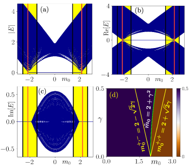
Figure 1: We show $\lvert E\rvert$, ${\rm Re}[E]$, and ${\rm Im}[E]$, obtained from real space Hamiltonian under OBC in all directions using Eq. (S1), as a function of $m_{0}$ in (a), (b), and (c), respectively. The mid-gap MZMs disappear into the bulk bands at $m_{0}={\tilde{m}_{0}}=\pm(t_{x}+t_{y}+{\gamma_{x}^{2}}/{2\lambda_{x}^{2}}+{\gamma_{y}^{2}}/{2\lambda_{y}^{2}})$, defined by the red lines. The EPs $m_{0}^{s,\pm}=s(t_{x}+t_{y})\pm\sqrt{\gamma_{x}^{2}+\gamma_{y}^{2}}$ with $s=\pm$ are marked by black lines within which ${\rm Re}[E(k)]$ associated with $\mathcal{H}(\boldsymbol{\mathrm{k}})$ remains gapless as designated by yellow-shaded region. (d) The topological phase diagram is depicted in the $m_{0}\mathchar 45\relax\gamma$ plane using nested polarization $\langle\nu_{y,\mu^{\prime}}^{\nu_{x}}\rangle$ Eq. (7). The yellow and green lines correspond to $m_{0}^{+,\pm}$ and ${\tilde{m}_{0}}$, respectively while the later separates SOTSC phase $\langle\nu_{y,\mu^{\prime}}^{\nu_{x}}\rangle=0.5$ from the trivial phase $\langle\nu_{y,\mu^{\prime}}^{\nu_{x}}\rangle=0.0$. The parameters used here are $t_{x}=t_{y}=\lambda_{x}=\lambda_{y}=\Delta=1.0$ and $\gamma_{x}=\gamma_{y}=0.4$.

The Hermitian system $\mathcal{H}^{\rm H}(\boldsymbol{\mathrm{k}})$ hosts zero-energy Majorana corner modes, protected by the TRS, in SOTSC phase for $m_{0}<\lvert t_{x}+t_{y}\rvert$ while trivially gapped for $m_{0}>\lvert t_{x}+t_{y}\rvert$ Yan et al. (2018). The NH system becomes defective at EPs provided $\lvert E(\boldsymbol{\mathrm{k}}_{\rm EP})\rvert=0$ which is in a complete contrast to the Hermitian system with $E(\boldsymbol{\mathrm{k}})=0$ at gapless point. A close inspection of Eq. (S1) suggests that four-fold degenerate energy bands yield $\lvert E(0,0)\rvert=0$ [$\lvert E(\pi,\pi)\rvert=0$] for $m_{0}^{+,\pm}=t_{x}+t_{y}\pm\sqrt{\gamma_{x}^{2}+\gamma_{y}^{2}}$ [$m_{0}^{-,\pm}=-t_{x}-t_{y}\pm\sqrt{\gamma_{x}^{2}+\gamma_{y}^{2}}$]. As a result, the gapless phase boundaries $m^{s}_{0}=s(t_{x}+t_{y})$ for the Hermitian case are modified in the present NH case with $m_{0}^{s,\pm}=s(t_{x}+t_{y})\pm\sqrt{\gamma_{x}^{2}+\gamma_{y}^{2}}$; where, $s=\pm$ (see black lines in Figs. 1 (a)-(c)). This refers to the fact that ${\rm Re}[E(\boldsymbol{\mathrm{k}})]$ is gapless for $m_{0}^{\pm,-}<m_{0}<m_{0}^{\pm,+}$ (see yellow-shaded region in Figs. 1 (a)-(c)). Furthermore, $\mathcal{H}(\boldsymbol{\mathrm{k}})$ is expected to be gapped in real sector of energy for $m_{0}^{-,+}<m_{0}<m_{0}^{+,-}$, hosting NH SOTSC phase.

The above conjecture, based on periodic boundary condition (PBC), is drastically modified when the NH system (S1) is investigated under OBC. We show $|E|$, ${\rm Re}[E]$ and ${\rm Im}[E]$ under OBC with blue points in Figs. 1 (a), (b), and (c), respectively. Surprisingly, the MZMs continue to survive inside the yellow-shaded region i.e., beyond $m_{0}=m_{0}^{-,+}$ and $m_{0}=m_{0}^{+,-}$, till $m_{0}<\rvert\tilde{m}_{0}\rvert=t_{x}+t_{y}+{\gamma_{x}^{2}}/{2\lambda_{x}^{2}}+{\gamma_{y}^{2}}/{2\lambda_{y}^{2}}$, depicted by the red line, where the ${\rm Re}[E]$ becomes gapless. All together this suggests the break-down of conventional BBC due to the non-Bloch nature of the NH Hamiltonian Yao and Wang (2018); Koch and Budich (2020); Zirnstein et al. (2021); Takane (2021). This apparent ambiguity in BBC affects the calculation of topological invariants, which we investigate below.

Fig. 2 (a) demonstrates the complex-energy profile ${\rm Im}[E]$ vs ${\rm Re}[E]$ of Hamiltonian (S1) in real space for $m_{0}<\rvert\tilde{m}_{0}\rvert$. We find the line gap for the NH system irrespective of the boundary conditions as the complex-energy bands do not cross a reference line in the complex-energy plane. The origin, marked with red dot in Fig. 2 (a), indicates the MZMs under OBC that are further shown the by the eight mid-gap states in ${\rm Re}[E]$-$m$ (state index) plot (see Fig. 2 (b)). Analyzing the local density of states (LDOS) of the above MZMs, we find sharp localization only at one corner out of the four corners Liu et al. (2019) (see Fig. 2 (c)). This is a consequence of the mirror-rotation symmetries $\mathcal{M}_{xy}$ or $\mathcal{M}_{x\bar{y}}$ even though MZMs spatially coincide. There might be additional protection from the bulk modes coming due to the emergent short-range nature of the superconducting gap Viyuela et al. (2016). The MZMs are localized over more than a single corner when $\mathcal{M}_{xy}$ or $\mathcal{M}_{x\bar{y}}$ is broken sup . The MZMs are also found to be robust against onsite disorder that respects mirror-rotation and chiral symmetries (see supplemental material sup ). In addition, we remarkably find that the LDOS of the bulk modes also exhibits substantial corner localization as depicted in the insets of Fig. 2(c) Yao and Wang (2018); Kunst et al. (2018); Helbig et al. (2020). The above features, reflecting the non-Block nature of the system, are referred to as the NH skin effect Yao and Wang (2018); Kunst et al. (2018). This is in contrast to the Hermitian case where only the zero-energy modes can populate four corners of the 2D square lattice Schindler et al. (2018); Nag et al. (2019); Ghosh et al. (2020).

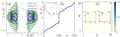
Figure 2: (a) The eigenvalue spectrum for the real space 2D system Eq. (S1), obeying PBC in both direction (black dots), PBC in $y$ and OBC in $x$-direction (green dots), and OBC in both directions (blue dots) are depicted in complex energy plane. The zero-energy mode, obtained from OBC, is marked by red dots. (b) ${\rm Re}[E_{m}]$ as a function of the state index $m$ is displayed where eight mid-gap MZMs are highlighted in the inset. (c) The LDOS, associated with eight MZMs in (b), show sharp localization only at one corner. The LDOS for typical bulk states are shown in insets I1 (for $E_{m}=-2.631839$) and I2 (for $E_{m}=-1.738466+0.130006i$). We use $m_{0}=1.0$, while other parameters are same as Fig. 1.

Topological characterization.— To this end, in order to compute the topological invariant from ${\mathcal{H}}(\boldsymbol{\mathrm{k}})$ characterizing the SOTSC phase under OBC, we exploit the non-Bloch nature. We need to use the complex wave-vectors to describe open-boundary eigenstates such that $\boldsymbol{\mathrm{k}}\rightarrow\boldsymbol{\mathrm{k^{\prime}}}+i\boldsymbol{\mathrm{\beta}}$ with $\beta_{i}={\gamma_{i}}/{\lambda_{i}}$ ($i=x,y$) Yao et al. (2018). Upon replacing $k_{x,y}\rightarrow k_{x,y}^{\prime}-{i\gamma_{x,y}}/{\lambda_{x,y}}$, the renormalized topological mass $m^{\prime}_{0}$ acquires the following form in the limit $k_{x,y}\to 0$ and $\gamma_{x,y}\to 0$

$$m^{\prime}_{0}=m_{0}-t_{x}-t_{y}-\frac{\gamma_{x}^{2}}{2\lambda_{x}^{2}}-\frac{\gamma_{y}^{2}}{2\lambda_{y}^{2}}\ .$$ (2)

Note that $|{\tilde{m}_{0}}|=|m^{\prime}_{0}-m_{0}|$ denotes phase boundary of the SOTSC phase as obtained from Fig. 1 (b). Employing $\boldsymbol{\mathrm{k^{\prime}}}\rightarrow\boldsymbol{\mathrm{k^{\prime}}}$ in $\mathcal{H}(\boldsymbol{\mathrm{k}})$ i.e., $\mathcal{H}(\boldsymbol{\mathrm{k}})\to\mathcal{H}^{\prime}(\boldsymbol{\mathrm{k^{\prime}}})$, we construct the Wilson loop operator as Benalcazar et al. (2017b); Ghosh et al. (2022b)

$$W_{x,\boldsymbol{\mathrm{k^{\prime}}}}=F_{x,\boldsymbol{\mathrm{k^{\prime}}}+(L_{x}-1)\Delta_{x}\boldsymbol{\mathrm{e}}_{x}}(t)\cdots F_{x,\boldsymbol{\mathrm{k^{\prime}}}+\Delta_{x}\boldsymbol{\mathrm{e}}_{x}}F_{x,\boldsymbol{\mathrm{k^{\prime}}}}\$$ (3)

from the non-Bloch NH Hamiltonian $\mathcal{H}^{\prime}(\boldsymbol{\mathrm{k^{\prime}}})$ Shen et al. (2018); Esaki et al. (2011). We define $\left[F_{x,\boldsymbol{\mathrm{k^{\prime}}}}\right]_{mn}=\braket{\Psi^{\rm L}_{m}(\boldsymbol{\mathrm{k^{\prime}}}+\Delta_{x}\boldsymbol{\mathrm{e}}_{x})}{\Psi^{\rm R}_{n}(\boldsymbol{\mathrm{k^{\prime}}})}$, where $\ket{\Psi^{\rm R}_{m}(\boldsymbol{\mathrm{k^{\prime}}})}$ ($\bra{\Psi^{\rm L}_{m}(\boldsymbol{\mathrm{k^{\prime}}})}$) represents the occupied right (left) eigenvectors of the Hamiltonian $\mathcal{H}^{\prime}(\boldsymbol{\mathrm{k^{\prime}}})$ such that ${\rm Re}[E^{\prime}_{m}(\boldsymbol{\mathrm{k^{\prime}}})]<0$; $\Delta_{i}=2\pi/L_{i}$, with $L_{i}$ being the the number of discrete points considered along $i$-th direction and $\boldsymbol{\mathrm{e}}_{i}$ being the unit vector along the said direction. Notice that, the bi-orthogonalization guarantees the following $\sum_{n}\ket{\Psi^{\rm R}_{n}(\boldsymbol{\mathrm{k^{\prime}}})}\bra{\Psi^{\rm L}_{n}(\boldsymbol{\mathrm{k^{\prime}}})}=\mathbb{I}$ and $\langle\Psi^{\rm L}_{n}(\boldsymbol{\mathrm{k^{\prime}}})|\Psi^{\rm R}_{n}(\boldsymbol{\mathrm{k^{\prime}}})\rangle=\delta_{mn}$; where, $n$ runs over all the energy levels irrespective of their occupations. The first-order polarization $\nu_{x,\mu}(k_{y}^{\prime})$ is obtained from the eigenvalue equation for $W_{x,\boldsymbol{\mathrm{k^{\prime}}}}$ as follows

$$W_{x,\boldsymbol{\mathrm{k^{\prime}}}}\ket{\nu^{\rm R}_{x,\mu}(\boldsymbol{\mathrm{k^{\prime}}})}=e^{-2\pi i\nu_{x,\mu}(k_{y}^{\prime})}\ket{\nu^{\rm R}_{x,\mu}(\boldsymbol{\mathrm{k^{\prime}}})}\ .$$ (4)

Note that unlike the Hermitian case, here $W_{x,\boldsymbol{\mathrm{k^{\prime}}}}$ is no longer unitary resulting in $\nu_{x,\mu}(k_{y}^{\prime})$ to be a complex number Luo and Zhang (2019). Importantly, $\ket{\nu^{\rm R}_{x,\mu}(\boldsymbol{\mathrm{k^{\prime}}})}$ ($\bra{\nu^{\rm L}_{x,\mu}(\boldsymbol{\mathrm{k^{\prime}}})}$) designates bi-orthogonalized right (left) eigenvector of $W_{x,\boldsymbol{\mathrm{k^{\prime}}}}$ associated with $\mu=1,\cdots,4$-th eigenvalue. For a (second-order topological) SOT system, the real part of first-order polarization exhibits a finite gap in spectra such that it can be divided into two sectors as $\pm\nu_{x}(k_{y}^{\prime})$ where each sector is two-fold degenerate. Such a structure of Wannier centres in the non-Bloch case might be relied on the mirror symmetry of the underlying Hermitian Hamiltonian Benalcazar et al. (2017b); Ghosh et al. (2022b). In order to characterize the SOT phase, we calculate the polarization along the perpendicular $y$-direction by projecting onto each $\pm\nu_{x}$ branch. This allows us to employ the nested Wilson loop as follows Benalcazar et al. (2017b); Ghosh et al. (2022b)

$$W_{y,\boldsymbol{\mathrm{k^{\prime}}}}^{\pm\nu_{x}}=F_{y,\boldsymbol{\mathrm{k^{\prime}}}+(L_{y}-1)\Delta_{y}\boldsymbol{\mathrm{e}}_{y}}^{\pm\nu_{x}}\cdots F_{y,\boldsymbol{\mathrm{k^{\prime}}}+\Delta_{y}\boldsymbol{\mathrm{e}}_{y}}^{\pm\nu_{x}}F_{y,\boldsymbol{\mathrm{k^{\prime}}}}^{\pm\nu_{x}}\ .$$ (5)

Here, $\left[F_{y,\boldsymbol{\mathrm{k^{\prime}}}}^{\pm\nu_{x}}\right]_{\mu_{1}\mu_{2}}=\sum_{mn}\left[\nu^{\rm L}_{x,\mu_{1}}(\boldsymbol{\mathrm{k^{\prime}}}+\Delta_{y}\boldsymbol{\mathrm{e}}_{y})\right]^{*}_{m}\left[F_{y,\boldsymbol{\mathrm{k^{\prime}}}}\right]_{mn}$ $\left[\nu^{\rm R}_{x,\mu_{2}}(\boldsymbol{\mathrm{k^{\prime}}})\right]_{n}$ with $\left[F_{y,\boldsymbol{\mathrm{k^{\prime}}}}\right]_{mn}=\braket{\Psi^{\rm L}_{m}(\boldsymbol{\mathrm{k^{\prime}}}+\Delta_{y}\boldsymbol{\mathrm{e}}_{y})}{\Psi^{R}_{n}(\boldsymbol{\mathrm{k^{\prime}}})}$. The indices $\mu_{1,2}\in\pm\nu_{x}$ run over the projected eigenvectors of $W_{x,\boldsymbol{\mathrm{k^{\prime}}}}$ only. We evaluate $W_{y,\boldsymbol{\mathrm{k^{\prime}}}}^{\pm\nu_{x}}$ for a given value of $k^{\prime}_{x}$ that is the base point while calculating $W_{x,\boldsymbol{\mathrm{k^{\prime}}}}$ (3).

The nested polarization $\nu_{y,\mu^{\prime}}^{\pm\nu_{x}}(k_{x}^{\prime})$ can be extracted by solving the eigenvalue equation for $W_{y,\boldsymbol{\mathrm{k^{\prime}}}}^{\pm\nu_{x}}$

$$W_{y,\boldsymbol{\mathrm{k^{\prime}}}}^{\pm\nu_{x}}\ket{\nu_{y,\mu^{\prime}}^{{\rm R},\pm\nu_{x}}(\boldsymbol{\mathrm{k^{\prime}}})}=e^{-2\pi i\nu_{y,\mu^{\prime}}^{\pm\nu_{x}}(k_{x}^{\prime})}\ket{\nu_{y,\mu^{\prime}}^{{\rm R},\pm\nu_{x}}(\boldsymbol{\mathrm{k^{\prime}}})}\ .$$ (6)

The average nested Wannier sector polarization $\langle\nu_{y,\mu^{\prime}}^{\pm\nu_{x}}\rangle$ for the $\mu^{\prime}$-th branch, characterizing the 2D SOTSC, is given by

$$\langle\nu_{y,\mu^{\prime}}^{\pm\nu_{x}}\rangle=\frac{1}{L_{x}}\sum_{k_{x}^{\prime}}{\rm Re}\left[\nu_{y,\mu^{\prime}}^{\pm\nu_{x}}(k_{x}^{\prime})\right]\ .$$ (7)

We explore the SOT phase diagram by investigating mod($\langle\nu_{y,\mu^{\prime}}^{\pm\nu_{x}}\rangle,1.0$) in the $m_{0}\mathchar 45\relax\gamma$ ($\gamma_{x}=\gamma_{y}=\gamma$) plane keeping $t_{x}=t_{y}=\lambda_{x}=\lambda_{y}=1$ (see Fig. 1(d)). The blue (brown) region indicates the SOTSC and trivial phase. The green line in Fig. 1 (d), separating the above two phases, represents the phase boundary $\tilde{m}_{0}=2+\gamma^{2}$ as demonstrated in Eq. (2). On the other hand, the phase boundaries, obtained from bulk Hamiltonian (S1), are found to be $m_{0}^{+,\pm}=2\pm\sqrt{2}\gamma$ that are depicted by yellow lines in Fig. 1 (d). Therefore, the topological invariant, computed using the non-Bloch Hamiltonian $\mathcal{H}^{\prime}(\boldsymbol{\mathrm{k^{\prime}}})$, can accurately predict the MZMs as obtained from the real space Hamiltonian under OBC (see Fig. 1 (c)). This correspondence for very higher values of $\gamma$ no longer remains appropriate due to the possible break down of Eq. (2). Even though $M_{x,y}$ are broken, $\langle\nu_{y,\mu^{\prime}}^{\pm\nu_{x}}\rangle$ ($\langle\nu_{x,\mu^{\prime}}^{\pm\nu_{y}}\rangle$) yields half-integer quantization provided $\mathcal{M}_{xy}$ ($\mathcal{M}_{x\bar{y}}$) is preserved. Note that based on mirror rotation and sublattice symmetries, the NH SOTSC can be shown to exhibit integer quantization in winding number similar to NH SOTI Liu et al. (2019) (see supplemental material sup ).

Floquet generation of NH SOTSC.— Having studied the static NH SOTSC, we seek the answer to engineer dynamic NH SOTSC out of trivial phase by periodically kicking the on-site mass term of the Hamiltonian $\mathcal{H}(\boldsymbol{\mathrm{k}})$ (Eq. (S1)) as Ghosh et al. (2021c, 2022a)

$$m(t)=m_{1}\sum_{r=-\infty}^{\infty}\delta\left(t-rT\right)\ .$$ (8)

Here, $m_{1}$ and $T$ represent the strength of the drive and the time-period, respectively. The Floquet operator is formulated to be

$$U(\boldsymbol{\mathrm{k}},T) = {\rm TO}\exp\left[-i\int_{0}^{T}dt\left\{\mathcal{H}(\boldsymbol{\mathrm{k}})+m(t)\Gamma_{3}\right\}\right]$$ (9)

$$= \exp\left[-i\mathcal{H}(\boldsymbol{\mathrm{k}})T\right]\exp\left[-im_{1}{\color[rgb]{1,0,0}\Gamma_{3}}\right]\ ,$$

where TO denotes the time ordering. Notice that $m_{0}>|t_{x}+t_{y}+\sqrt{\gamma_{x}^{2}+\gamma_{y}^{2}}|$ such that the underlying static NH Hamiltonian $\mathcal{H}(\boldsymbol{\mathrm{k}})$ remains in the trivially gapped phase. Having constructed the Floquet operator $U(\boldsymbol{\mathrm{k}},T)$, we resort to OBCs and diagonalize the Floquet operator to obtain the quasi-energy spectrum for the system. We depict the real part of the quasi-energy $\mu_{m}$ as function of the state index $m$ in Fig. 3 (a) where frequency of the drive is higher than the band-width of the system. The existence of eight MZMs is a signature of the NH Floquet SOTSC phase. The LDOS for the MZMs displays substantial localization only at one corner in Fig. 3(b). Insets show the NH skin effect where the bulk modes at finite energy also have a fair amount of corner localization.

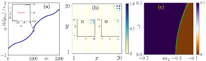
Figure 3: (a) The real part of the quasi-energy spectrum $E_{m}$, obtained from Eq. (9) under OBC, are shown with eight Floquet Majorana $0$-modes in the inset. (b) The LDOS, associated with eight MZMs in (a), exhibits substantial localization only at one corner similar to Fig. 2 (c). The LDOS for typical bulk modes with $E_{m}=-0.697702\pi$ and $-0.453177\pi$ are demonstrated in insets I1 and I2. (c) The topological phase diagram is depicted in the $m_{1}\mathchar 45\relax\gamma$ plane where the Floquet SOTSC phase is characterized by the average Floquet nested Wannier sector polarization $\langle\nu_{y,\mu^{\prime}}^{{\rm F},\nu_{x}}\rangle=0.5$ (blue region). The phase boundary, marked by green line, is consistent with Eq. (11). We consider $m_{0}=2.5,~{}m_{1}=-0.4,~{}\Omega=10.0$ such that we start from the trivial phase deep inside the brown region in Fig. 1 (c).

In order to topologically characterize the above MZMs, we again make use of the non-Bloch form. Instead of the static Hamiltonian, we derive the high-frequency effective Floquet Hamiltonian, in the limit $T\rightarrow 0$ and $m_{1}\rightarrow 0$ to analyze the situation

$$H_{\rm Flq}(\boldsymbol{\mathrm{k}}) \approx \mathcal{H}(\boldsymbol{\mathrm{k}})+\frac{m_{1}}{T}\Gamma_{1}+m_{1}\sum_{j=2}^{4}N_{j}\Gamma_{j1}\ ,$$ (10)

with $\Gamma_{21}=-\sigma_{y}s_{z},\Gamma_{31}=\sigma_{x},\Gamma_{41}=-\tau_{y}\sigma_{z}$. Upon substitution of $\boldsymbol{\mathrm{k}}\rightarrow\boldsymbol{\mathrm{k^{\prime}}}+i\boldsymbol{\mathrm{\beta}}$, the modified mass term in $H^{\prime}_{\rm Flq}(\boldsymbol{\mathrm{k^{\prime}}})$ reads as

$$m^{\prime}_{0}=m_{0}-t_{x}-t_{y}-\frac{\gamma_{x}^{2}}{2\lambda_{x}^{2}}-\frac{\gamma_{y}^{2}}{2\lambda_{y}^{2}}+\frac{m_{1}}{T}\ .$$ (11)

Evaluating the effective Floquet nested Wannier sector polarization $\langle\nu_{y,\mu^{\prime}}^{{\rm F},\pm\nu_{x}}\rangle$ numerically from non-Bloch Floquet operator $U^{\prime}(\boldsymbol{\mathrm{k^{\prime}}},T)$ Ghosh et al. (2022b); Huang and Liu (2020), we obtain the Floquet phase diagram in $m_{1}$-$\gamma$ plane as shown in Fig. 3 (c). The non-Bloch Floquet operator can be considered as the dynamic analog of the non-Bloch NH Hamiltonian $H^{\prime}(\boldsymbol{\mathrm{k^{\prime}}})$. In particular, we use bi-orthogonalized $\ket{\Psi^{\rm R}_{\rm F}(\boldsymbol{\mathrm{k^{\prime}}})}$ ($\bra{\Psi^{\rm L}_{\rm F}(\boldsymbol{\mathrm{k^{\prime}}})}$), representing the occupied right (left) quasi-states of $U^{\prime}(\boldsymbol{\mathrm{k^{\prime}}},T)$ with quasi-energy $-\pi/T<{\rm Re}[\mu]<0$, to construct the Wilson loops $W^{\rm F}_{x,\boldsymbol{\mathrm{k^{\prime}}}}$ for the driven case. Following identical line of arguments, presented for the static case, $W_{y,\boldsymbol{\mathrm{k^{\prime}}}}^{{\rm F},\pm\nu_{x}}$ is obtained from $\left[F_{y,\boldsymbol{\mathrm{k^{\prime}}}}^{{\rm F},\pm\nu_{x}}\right]_{\mu_{1}\mu_{2}}=\sum_{mn}\left[\nu^{{\rm F},\rm L}_{x,\mu_{1}}(\boldsymbol{\mathrm{k^{\prime}}}+\Delta_{y}\boldsymbol{\mathrm{e}}_{y})\right]^{*}_{m}\left[F^{\rm F}_{y,\boldsymbol{\mathrm{k^{\prime}}}}\right]_{mn}$ $\left[\nu^{{\rm F},\rm R}_{x,\mu_{2}}(\boldsymbol{\mathrm{k^{\prime}}})\right]_{n}$ with $\left[F^{\rm F}_{y,\boldsymbol{\mathrm{k^{\prime}}}}\right]_{mn}=\braket{\Psi^{\rm L}_{{\rm F}m}(\boldsymbol{\mathrm{k^{\prime}}}+\Delta_{y}\boldsymbol{\mathrm{e}}_{y})}{\Psi^{R}_{{\rm F}n}(\boldsymbol{\mathrm{k^{\prime}}})}$ and $\ket{\nu^{\rm F,R}_{x,\mu}(\boldsymbol{\mathrm{k^{\prime}}})}$ ($\bra{\nu^{\rm F,L}_{x,\mu}(\boldsymbol{\mathrm{k^{\prime}}})}$) designates bi-orthogonalized right (left) eigenvector of $W^{\rm F}_{x,\boldsymbol{\mathrm{k^{\prime}}}}$. Interestingly, this is similar to the static phase diagram where the phase boundary is accurately explained by Eq. (11).

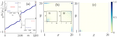
Figure 4: (a) We repeat Fig. 3 (a) considering the low frequency mass-kick with $\Omega=5.0$ where we find eight regular $0$- and anomalous $\pi$-modes simultaneously. We show the LDOS associated with ${\rm Re}[E_{m}]=0$- and ${\rm Re}[E_{m}]=+\pi$ in (b) and (c), respectively. The LDOS for Floquet bulk modes with $E_{m}=-0.838779\pi-0.085397\pi i$ and $-0.471932\pi$ are respectively depicted in the insets I1 and I2 of (b). We consider $m_{0}=0,m_{1}=1.5,\Omega=5.0$.

We further analyze the problem for lower frequency regime to look for anomalous Floquet modes at quasienergy ${\rm Re}[\mu]=\pm\pi$ Ghosh et al. (2022a, b). We depict one such scenario for $\Omega=2\pi/T=5.0$ in Fig. 4 (a) where eight anomalous $\pi$-modes appear simultaneously with regular eight $0$-modes. The corresponding LDOS for $0$-mode and $\pi$-mode are shown in Fig. 4(b) and (c), respectively. Interestingly, the $0$-mode and the $\pi$-mode populate different corners of the system. As a signature of NH skin effect, we show the LDOS for two bulk states in the inset I1 and I2 of Fig. 4(b). The localization profile of the zero-energy states and bulk states are unique to the NH system that can not be explored in its Hermitian counterpart.

Discussions.— The number of MZMs can be tuned in our case by the application of magnetic field similar to the Hermitian SOTSC phase Ghosh et al. (2021c). The long-range hopping provides another route to enhance the number of MZMs that can in principle be applicable for the non-Hermitian case as well DeGottardi et al. (2013); Benalcazar and Cerjan (2022). Interestingly, Floquet driving delivers an alternative handle to generate long-range hopping effectively out of the short-range NH model such that the number of MZMs are varied (see supplemental material sup ). Interestingly, Hermitian and non-Hermitian phases belong to the Dirac and non-Hermitian Dirac universality classes Chen et al. (2017); Arouca et al. (2020). In the case of HOT phases, one expects different critical exponents with respect to the usual Dirac model. The breakdown of BBC and skin effect are intimately related to such non-Hermitian Dirac universality class. The edge theory, computed from Hermitian HOT model, is modified due to the non-Hermiticity with the possible non-Bloch form. Given the experimental realization of spin-orbit coupling Huang et al. (2016); Wu et al. (2016), non-Hermiticity Li et al. (2019); Song et al. (2019) and theoretical proposals on topological superfluidity Jia et al. (2019); Bühler et al. (2014) in optical lattice, we believe that the cold atom systems might be a suitable platform for the potential experimental realization of our findings Makris et al. (2008); Miyake et al. (2013); McKay and DeMarco (2011). However, we note that the superconductivity might be hard to achieve in the NH setting.

Summary and conclusions.— In this article, we consider 2D NH TI, proximized with $d$-wave superconductivity, to investigate the emergence of NH SOTSC phase. From the analysis of EPs on the bulk NH Hamiltonian under PBC, one can estimate the gapped and gapless phase in terms of the real energies (see Fig. 1). By contrast, the MZMs, obtained from the real space NH Hamiltonian under OBC, do not immediately vanish inside the bulk gapless region (see Fig. 2). This apparent breakdown of the BBC can be explained by the non-Bloch nature of the NH Hamiltonian that further results in the MZMs residing at only one corner while the bulk modes populate the boundaries. While the later is dubbed as NH skin effect. We propose the nested polarization for topologically characterize the MZMs upon exploiting the non-Bloch form of the complex wave vectors. This resolves the anomaly between the phase boundaries, obtained from OBC and PBC, in the topological phase diagram. Finally, we adopt a mass-kick drive to illustrate the Floquet generation of NH SOTSC out of the trivial phase and characterize it using non-Bloch Floquet nested Wannier sector polarization (see Fig. 3). In addition, we demonstrate the emergence of anomalous $\pi$-mode following such drive when the frequency is lowered (see Fig. 4). The mirror symmetries $M_{x,y}$ play crucial role in characterizing the anomalous $\pi$-modes Huang and Liu (2020); Ghosh et al. (2022b). Therefore, such characterization in the absence of mirror symmetries is a future problem.

Acknowledgments.— A.K.G. acknowledges SAMKHYA: High-Performance Computing Facility provided by Institute of Physics, Bhubaneswar, for numerical computations. We thank Arijit Saha for useful discussions.

S1 Underlying spatial symmetry

In this section, we analyze the crystalline symmetries associated with the non-Hermitian (NH) second-order topological superconductor (SOTSC) as presented in Eq. (1) of the main text. In order to understand the spatial symmetry of the model, we first analyze the underlying Hermitian version of our model $\mathcal{H}^{\rm H}(\boldsymbol{\mathrm{k}})=\lambda_{x}\sin k_{x}\tau_{z}\sigma_{x}s_{z}+\lambda_{y}\sin k_{y}\tau_{z}\sigma_{y}s_{0}+(m_{0}-t_{x}\cos k_{x}-t_{y}\cos k_{y})\tau_{z}\sigma_{z}s_{0}+\Delta(\cos k_{x}-\cos k_{y})\tau_{x}\sigma_{0}s_{0}$ as demonstrated in Eq. (1) of the main text. The Hermitian Hamiltonian obeys the following spatial symmetries-

• mirror symmetry along $x$ with $\mathcal{M}_{x}=\tau_{x}\sigma_{x}s_{0}$: $\mathcal{M}_{x}\mathcal{H}^{\rm H}(k_{x},k_{y})\mathcal{M}_{x}^{-1}=\mathcal{H}^{\rm H}(-k_{x},k_{y})$,

• mirror symmetry along $y$ with $\mathcal{M}_{y}=\tau_{x}\sigma_{y}s_{0}$: $\mathcal{M}_{y}\mathcal{H}^{\rm H}(k_{x},k_{y})\mathcal{M}_{y}^{-1}=\mathcal{H}^{\rm H}(k_{x},-k_{y})$,

• four-fold rotation with $C_{4}=\tau_{z}e^{-\frac{i\pi}{4}\sigma_{z}s_{z}}$: $C_{4}\mathcal{H}^{\rm H}(k_{x},k_{y})C_{4}^{-1}=\mathcal{H}^{\rm H}(-k_{y},k_{x})$, if $t_{x}=t_{y}$ and $\lambda_{x}=\lambda_{y}$,

• mirror rotation I with $\mathcal{M}_{xy}=C_{4}\mathcal{M}_{y}$: $\mathcal{M}_{xy}\mathcal{H}^{\rm H}(k_{x},k_{y})\mathcal{M}_{xy}^{-1}=\mathcal{H}^{\rm H}(k_{y},k_{x})$, if $t_{x}=t_{y}$ and $\lambda_{x}=\lambda_{y}$,

• mirror rotation II with $\mathcal{M}_{x\bar{y}}=C_{4}\mathcal{M}_{x}$: $\mathcal{M}_{x\bar{y}}\mathcal{H}^{\rm H}(k_{x},k_{y})\mathcal{M}_{x\bar{y}}^{-1}=\mathcal{H}^{\rm H}(-k_{y},-k_{x})$, if $t_{x}=t_{y}$ and $\lambda_{x}=\lambda_{y}$,

• sublattice/ chiral symmetry with $\mathcal{S}=\tau_{y}\sigma_{0}s_{0}$: $\mathcal{S}\mathcal{H}^{\rm H}(\boldsymbol{\mathrm{k}})\mathcal{S}^{-1}=-\mathcal{H}^{\rm H}(\boldsymbol{\mathrm{k}})$.

The extended Hermitian Hamiltonian $\tilde{\mathcal{H}}(\boldsymbol{\mathrm{k}})$ is found to be crucial for analyzing the crystalline symmetries of the NH Hamiltonian that can be wriiten as follows Kawabata et al. (2020)

$$\tilde{\mathcal{H}}(\boldsymbol{\mathrm{k}})=\begin{pmatrix}0&\mathcal{H}(\boldsymbol{\mathrm{k}})\\ \mathcal{H}(\boldsymbol{\mathrm{k}})^{\dagger}&0\ \\ \end{pmatrix}\ .$$ (S1)

To be precise, $\tilde{\mathcal{H}}(\boldsymbol{\mathrm{k}})=\lambda_{x}\sin k_{x}\mu_{x}\tau_{z}\sigma_{x}s_{z}+\gamma_{x}\mu_{y}\tau_{z}\sigma_{x}s_{z}+\lambda_{y}\sin k_{y}\mu_{x}\tau_{z}\sigma_{y}s_{0}+\gamma_{y}\mu_{y}\tau_{z}\sigma_{y}s_{0}+(m_{0}-t_{x}\cos k_{x}-t_{y}\cos k_{y})\mu_{x}\tau_{z}\sigma_{z}s_{0}+\Delta(\cos k_{x}-\cos k_{y})\mu_{x}\tau_{x}\sigma_{0}s_{0}$. For $\gamma_{x}\neq 0,\gamma_{y}=0$ ($\gamma_{x}=0,\gamma_{y}\neq 0$), $\tilde{\mathcal{H}}(\boldsymbol{\mathrm{k}})$ breaks $\mathcal{M}_{x}=\mu_{x}\tau_{x}\sigma_{x}s_{0}$ ($\mathcal{M}_{y}=\mu_{x}\tau_{x}\sigma_{y}s_{0}$). When $\gamma_{x}\neq 0,\gamma_{y}\neq 0$, $\tilde{\mathcal{H}}(\boldsymbol{\mathrm{k}})$ breaks $C_{4}=\mu_{x}\tau_{z}e^{-\frac{i\pi}{4}\sigma_{z}s_{z}}$. For $\gamma_{x}=\gamma_{y}\neq 0$, $\tilde{\mathcal{H}}(\boldsymbol{\mathrm{k}})$ preserves $\mathcal{M}_{xy}=C_{4}\mathcal{M}_{y}$ and $\mathcal{M}_{x\bar{y}}=C_{4}\mathcal{M}_{x}$. On the other hand, $\tilde{\mathcal{H}}(\boldsymbol{\mathrm{k}})$ preserves the chiral symmetry $\mathcal{S}=\mu_{0}\tau_{y}\sigma_{0}s_{0}$.

Therefore, the NH Hamiltonian (Eq. (1) of the main text) breaks and respects the following symmetries. When $\gamma_{x}\neq 0$ ($\gamma_{y}\neq 0$) $\mathcal{H}(\boldsymbol{\mathrm{k}})$ breaks $\mathcal{M}_{x}$ ($\mathcal{M}_{y}$) and when both $\gamma_{x,y}\neq 0$, $\mathcal{H}(\boldsymbol{\mathrm{k}})$ breaks $C_{4}$ symmetry. The Hamiltonian $\mathcal{H}(\boldsymbol{\mathrm{k}})$ obeys both $\mathcal{M}_{xy}$ and $\mathcal{M}_{x\bar{y}}$ provided $\gamma_{x}=\gamma_{y}$. $\mathcal{H}(\boldsymbol{\mathrm{k}})$ also preserves the sublattice/ chiral symmetry $\mathcal{S}$ like its Hermitian counterpart.

S2 Effect of asymmetric $\gamma$ and the localization of the Majorana zero-modes

In this section, we study the localization of the Majorana zero-modes (MZMs) for different values of $\gamma_{x}$ and $\gamma_{y}$ Liu et al. (2019). In Fig. 2 (c) of the main text, we demonstrate that the MZMs are located only at the top-right corner of the system when $\gamma_{x}=\gamma_{y}=\gamma$. However, one can choose $\gamma_{x}=-\gamma_{y}=\gamma$ ($\gamma_{y}=-\gamma_{x}=\gamma$), and following the calculation of the local density of states (LDOS), it turns out that the MZMs are now localized at the bottom-right [Fig. S1 (a)] (top-left [Fig. S1 (b)]) corner of the system. When $\gamma_{x}=\gamma_{y}=-\gamma$, the MZMs are localized at the bottom-left corner of the system [see Fig. S1 (c)]. However, if we break the mirror rotation symmetry $\mathcal{M}_{xy}$ by considering $\gamma_{x}\neq\gamma_{y}$, we depict that the MZMs are localized at more than one corner of the system in Fig. S1 (d) and (e). We obtain a non-quantized value for the topological invariant defined by employing the nested Wilson loop in the main text [Eq.(7)] when the mirror-rotation symmetry $\mathcal{M}_{xy}$ is broken. We can find that either right(left)-bottom or left(right)-top corner is only occupied for mirror-rotation symmetry $\mathcal{M}_{x\bar{y}}$ ($\mathcal{M}_{xy}$). Therefore, the localization profile of MZMs over a given corner is caused by the interplay between the mirror-rotation symmetry and non-Hermiticity Liu et al. (2019).

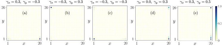
Figure S1: We depict the local density of states for the Majorana zero-modes as a function of the system dimensions in (a) for $\gamma_{x}=-\gamma_{y}=0.3$, (b) for $\gamma_{y}=-\gamma_{x}=0.3$, (c) for $\gamma_{x}=\gamma_{y}=-0.3$, (d) for $\gamma_{x}=0.0,\gamma_{y}=0.3$, and (e) for $\gamma_{x}=0.3,\gamma_{y}=0.5$. The other parameters used here are $t_{x}=t_{y}=\lambda_{x}=\lambda_{y}=\Delta=1.0$.

S3 Symmetry constraints for Wannier bands

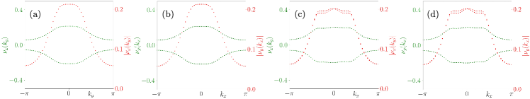
Figure S2: We exhibit the first-order Wannier centres $\nu_{x}(k_{y})$ (left axis) and $\lvert\nu_{x}(k_{y})\rvert$ (right axis) as function of $k_{y}$ in (a) for Hermitian case (c) for non-Hermitian case. In the non-Hermitian case the breaking of mirror symmetry $M_{x}$ causes the irreversible nature of first-order branches i.e.,  $\nu_{x}(k_{y})\not\to-\nu_{x}(k_{y})$, which is more evident from $\lvert\nu_{x}(k_{y})\rvert$. (b), (d) We repeat (a) and (b) for $\nu_{y}(k_{x})$. Note that for better visibility, we adopt the scale for $\nu_{x}(k_{y}),~{}\nu_{y}(k_{x})$ to be between $[-0.5,0.5]$ while $|\nu_{x}(k_{y})|,~{}|\nu_{y}(k_{x})|$ are bounded between $[0.0,0.22]$.

In this section, we show that how the first- and second-order Wannier centres behave under the above spatial symmetries. The first-order Wannier centres $\nu_{x}(k_{y})$ and second-order Wannier centres $\nu_{y}^{\nu_{x}}$ behave in the following way Benalcazar et al. (2017b)- mirror-rotation along $x$-direction $M_{x}$: $\nu_{x}(k_{y})\to-\nu_{x}(k_{y})$ [see Fig. S2], and $\nu_{y}^{\nu_{x}}(k_{x})\to\nu_{y}^{-\nu_{x}}(-k_{x})$; $M_{x}$ causes the first-order branches to appear in pairs, mirror-rotation along $y$-direction. $M_{y}$: $\nu_{x}(k_{y})\to\nu_{x}(-k_{y})$, and $\nu_{y}^{\nu_{x}}(k_{x})\to-\nu_{y}^{\nu_{x}}(k_{x})$; $M_{y}$ defines the shape of the first-order branches. The four-fold rotation $C_{4}$ and mirror rotations $\mathcal{M}_{xy}$, $\mathcal{M}_{x\bar{y}}$ interchange the branches, $C_{4}$: $\nu_{x}(k_{y})\to-\nu_{y}(k_{x})$, and $\nu_{y}^{\nu_{x}}(k_{x})\to\nu_{x}^{-\nu_{y}}(-k_{y})$, $\mathcal{M}_{xy}$: $\nu_{x}(k_{y})\to\nu_{y}(k_{x})$, and $\nu_{y}^{\nu_{x}}(k_{x})\to\nu_{x}^{\nu_{y}}(k_{y})$ $\mathcal{M}_{x\bar{y}}$: $\nu_{x}(k_{y})\to-\nu_{y}(-k_{x})$, and $\nu_{y}^{\nu_{x}}(k_{x})\to-\nu_{x}^{-\nu_{y}}(-k_{y})$. In our case, the first-order branches do not follow the above relations as $M_{x,y}$ symmetries are broken. However, the second-order polarization i.e., nested polarization mod($\langle\nu_{y,\mu^{\prime}}^{\pm\nu_{x}}\rangle,1.0$) and mod($\langle\nu_{x,\mu^{\prime}}^{\pm\nu_{y}}\rangle,1.0$) both are found to be $0.5$ following the mirror rotation symmetries generated by $\mathcal{M}_{xy}$ and $\mathcal{M}_{x\bar{y}}$. Moreover, under these mirror rotation symmetries, one can show that $\nu_{x}^{\nu_{y}}(k_{y})\to-\nu_{x}^{-\nu_{y}}(-k_{y})$ and $\nu_{y}^{\nu_{x}}(k_{x})\to-\nu_{y}^{-\nu_{x}}(-k_{x})$. We further notice that when $\mathcal{M}_{xy}$ is broken, $\langle\nu_{y,\mu^{\prime}}^{\pm\nu_{x}}\rangle$ and $\langle\nu_{x,\mu^{\prime}}^{\pm\nu_{y}}\rangle$ do not produce a quantized value of $0/0.5$. Therefore, these spatial symmetries can predict the quantization of the second-order polarization that determines the second-order topology. In this regard, we would like to comment that the winding number, based on the mirror rotation symmetry $\mathcal{M}_{xy}$ and the sublattice symmetry $\mathcal{S}$, is shown to topologically characterize the NH higher-order topological insulator (HOTI) Liu et al. (2019). We believe that it is possible to define such a winding number yielding quantized values in the SOTSC phase as our NH model preserves mirror rotation and sublattice symmetries.

Note that winding number, usually characterizing a first-order topological phase provided Hamiltonian preserves sublattice symmetry Chiu et al. (2016), can also identify a second-order topological phase while appropriately defined with other symmetry constraints. The winding number for a Hamiltonian physically means how many times the Hamiltonian encircles a given point when a parameter is cyclically varied. On the other hand, half integer eigenvalues of nested Wilson loop refers to the fact that Wannier centers, located at a high-symmetry point with respect to the mirror symmetries, lie half-way between the lattice sites for higher-order topological phase Benalcazar et al. (2017b). Therefore, both the above invariant captures the non-trivial nature of the underlying wave-functions in the Brillouin zone through either Wannier center or winding number once a certain set of symmetries is present. The winding number thus can be considered to be equivalent to our nested Wilson loop eigenvalues i.e, second-order Wannier values. The quantization in $\langle\nu_{y,\mu^{\prime}}^{\pm\nu_{x}}\rangle$ and $\langle\nu_{x,\mu^{\prime}}^{\pm\nu_{y}}\rangle$ might be intimately connected to winding number as stated above. However, the detailed mathematical proof is an open question yet, to the best of our knowledge, that we leave for future studies.

S4 $s$-wave NH SOTSC

In the main text, we discuss $d$-wave proximized to engineer NH SOTSC phase. We here illustrate that NH higher-order topological superconductor (HOTSC) can be contemplated for $s$-wave superconductivity with pairing amplitude $\Delta_{s}$ as follows Yan (2019a); Ghosh et al. (2021b) $\mathcal{H}(\boldsymbol{\mathrm{k}})=\boldsymbol{\mathrm{N}}\cdot\boldsymbol{\mathrm{\Gamma}}$; where, $\boldsymbol{\mathrm{N}}=\{\lambda_{x}\sin k_{x}+i\gamma_{x},\lambda_{y}\sin k_{y}+i\gamma_{y},m_{0}-t_{x}\cos k_{x}-t_{y}\cos k_{y},\Delta_{s},\Lambda(\cos k_{x}-\cos k_{y})\}$, $\boldsymbol{\mathrm{\Gamma}}=\{\tau_{z}\sigma_{x}s_{z},\tau_{z}\sigma_{y}s_{0},\tau_{z}\sigma_{z}s_{0},\tau_{x}\sigma_{0}s_{0},\tau_{0}\sigma_{x}s_{x}\}$. The last term proportional to $\Lambda$ represents $C_{4}$ symmetry breaking Wilson-Dirac mass term. We depict the corresponding complex-energy bands in complex energy plane, eigenvalue spectra highlighting the mid-gap states, and the LDOS associated to the MZMs and bulk modes in Fig. S3 (a), (b), and (c), respectively. The NH SOTSC phase with $\Delta_{s}$ can also be obtained using in-plane magnetic field instead of $C_{4}$ symmetry breaking Wu et al. (2020a); Ghosh et al. (2021b). The topological characterization of these phases we leave for future studies.

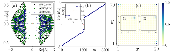
Figure S3: (a) The eigenvalue spectrum for the real space 2D system, obeying PBC in both direction (black dots), PBC in $y$ and OBC in $x$-direction (green dots), and OBC in both directions (blue dots) are depicted in complex energy plane. The zero-energy mode, obtained from OBC, is marked by red dots. (b) ${\rm Re}[E_{m}]$ as a function of the state index $m$ is displayed where eight mid-gap MZMs are highlighted in the inset. (c) The LDOS, associated with eight MZMs in (b), show sharp localization only at one corner. We choose $E_{m}=-2.666466$ and $E_{m}=-1.713832+0.038500i$ for insets I1 and I2 in (c), respectively. The parameters used here are $t_{x}=t_{y}=\lambda_{x}=\lambda_{y}=\Lambda=1.0$ and $\Delta_{s}=\gamma_{x}=\gamma_{y}=0.4$.

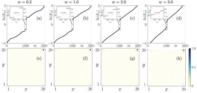
Figure S4: We depict the eigenvalue spectra $E_{m}$ and local density of states in (a), (e) for $w=0.2$, (b), (f) for $w=1.0$, (c), (g) for $w=2.0$, and (d), (h) for $w=3.0$. One see that even for a very high-disorder strength, the Majorana zero modes are roboust.

S5 Effect of onsite disorder

In this section, we investigate the effect of on-site disorder to investigate the stability of the MZMs. We consider an onsite disorder potential of the form $V(i,j)=\sum_{i,j}V_{ij}\Gamma_{3}$. Here, $V_{ij}$ is randomly distributed in the range $V_{ij}\in\left[-\frac{w}{2},\frac{w}{2}\right]$; while $w$ accounts for the strength of the disorder potential. The disordered NH Hamiltonian ${\mathcal{H}}^{\prime}(i,j)={\mathcal{H}}(i,j)+V(i,j)\Gamma_{3}$ respects the chiral symmetry while investigating the extended Hermitian Hamiltonian $\tilde{{\mathcal{H}}}^{\prime}$: $\mathcal{S}\tilde{{\mathcal{H}}}^{\prime}\mathcal{S}^{-1}=-\tilde{{\mathcal{H}}}^{\prime}$ with $\mathcal{S}=\mu_{0}\tau_{y}\sigma_{0}s_{0}$. We also note that on-site disorder preserves $\mathcal{M}_{xy}$. In the presence of the onsite disorder, the real-space Hamiltonian $\mathcal{H}^{\prime}$ is given as

$$\mathcal{H}^{\prime} = \sum_{i,j}\Psi_{i,j}^{\dagger}\left[i\gamma_{x}\Gamma_{1}i\gamma_{y}\Gamma_{2}+\left(m_{0}+V_{ij}\right)\Gamma_{3}\right]\Psi_{i,j}+\sum_{\langle i,j\rangle_{x}}\Psi_{i,j}^{\dagger}\left[-\frac{i\lambda_{x}}{2}\Gamma_{1}-\frac{t_{x}}{2}\Gamma_{3}+\frac{\Delta}{2}\Gamma_{4}\right]\Psi_{i,j}$$ (S2)

$$+\sum_{\langle i,j\rangle_{y}}\Psi_{i,j}^{\dagger}\left[-\frac{i\lambda_{y}}{2}\Gamma_{2}-\frac{t_{y}}{2}\Gamma_{3}-\frac{\Delta}{2}\Gamma_{4}\right]\Psi_{i,j}\ .$$

Here, $\Psi_{i,j}$ is a $8\times 1$ matrix consisting of the annihilation operator in the particle-hole, orbital, and spin subspace at a lattice site $(i,j)$. And $\langle i,j\rangle_{x}$ ($\langle i,j\rangle_{y}$) represents the nearest neighbor hopping along $x$ ($y$) direction. We consider 500 disorder configurations and depict the eigenstates $E_{m}$ as a function of the state index $m$ and the LDOS of the MZMs in Fig. S4 for different disorder strengths. The MZMs remain localized at a given corner due to the mirror symmetry preserving nature of the on-site disorder. We can conclude from the eigenvalue spectra and the LDOS plot that the MZMs are robust and against the onsite disorder.

S6 Tuning the number of MCMs dynamically

In this section, we discuss how Floquet engineering permits us to generate more in-gap states (both $0$- and $\pi$-gap) by tuning the different driving parameters suitably. The generation of multiple in-gap states is attributed to higher-order hoppings generated in the dynamical system. The mass-kick protocol, introduced in Eq. (9) of the main text, can be used to create multiple Majorana corner modes (MCMs). We depict the real part of the quasienergy spectra as a function of the driving frequency $\Omega$ in Fig. S5 (a). In order to understand the generation of the MCMs more clearly, we exemplify two cases in Fig. S5 (b) and (c) for $\Omega=4.6$ and $1.9$, respectively. In Fig. S5 (b), the number of $0$-MCMs is twice that of the static case, whereas the number of $\pi$-MCMs remains the same. While in Fig. S5 (c), the number of $\pi$-MCMs is thrice compared to the case in the main text (see Fig. 4 (a) of the main text).

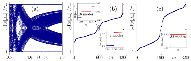
Figure S5: We depict the real part of the quasienergy spectra Re$[\mu_{m}]$ as function of the driving frequency $\Omega$ in (a). We exhibit the quasienergy spectra as function of the state index $m$ for two individual cases in (b) with 16 0-MCMs and 8 $\pi$-MCMs, and (b) 32 $\pi$-MCMs. We consider $\Omega=4.6$ for (b) and $\Omega=1.9$ for (c). While all the other parameters take the value: $m_{0}=0.0,~{}m_{1}=2.5$, $t_{x}=t_{y}=\lambda_{x}=\lambda_{y}=\Delta=1.0$, and $\gamma_{x}=\gamma_{y}=0.4$.

References

- Hasan and Kane (2010) M. Z. Hasan and C. L. Kane, “Colloquium: topological insulators,” Rev. Mod. Phys. 82, 3045 (2010).
- Haldane (1988) F. D. M. Haldane, “Model for a quantum hall effect without landau levels: Condensed-matter realization of the“parity anomaly”,” Phys. Rev. Lett. 61, 2015–2018 (1988).
- Kane and Mele (2005) C. L. Kane and E. J. Mele, “ topological order and the quantum spin hall effect,” Phys. Rev. Lett. 95, 146802 (2005).
- Bernevig et al. (2006) B. A. Bernevig, T. L. Hughes, and S.-C. Zhang, “Quantum spin hall effect and topological phase transition in hgte quantum wells,” Science 314, 1757–1761 (2006).
- Alicea (2012) J. Alicea, “New directions in the pursuit of majorana fermions in solid state systems,” Rep. Prog. Phys. 75, 076501 (2012).
- Beenakker (2013) C. Beenakker, “Search for majorana fermions in superconductors,” Annu. Rev. Condens. Matter Phys. 4, 113–136 (2013).
- Jotzu et al. (2014) G. Jotzu, M. Messer, R. Desbuquois, M. Lebrat, T. Uehlinger, D. Greif, and T. Esslinger, “Experimental realization of the topological haldane model with ultracold fermions,” Nature 515, 237–240 (2014).
- Das et al. (2012) A. Das, Y. Ronen, Y. Most, Y. Oreg, M. Heiblum, and H. Shtrikman, “Zero-bias peaks and splitting in an al–inas nanowire topological superconductor as a signature of majorana fermions,” Nat. Phys. 8, 887–895 (2012).
- Benalcazar et al. (2017a) W. A. Benalcazar, B. A. Bernevig, and T. L. Hughes, “Quantized electric multipole insulators,” Science 357, 61–66 (2017a).
- Benalcazar et al. (2017b) W. A. Benalcazar, B. A. Bernevig, and T. L. Hughes, “Electric multipole moments, topological multipole moment pumping, and chiral hinge states in crystalline insulators,” Phys. Rev. B 96, 245115 (2017b).
- Song et al. (2017) Z. Song, Z. Fang, and C. Fang, “-dimensional edge states of rotation symmetry protected topological states,” Phys. Rev. Lett. 119, 246402 (2017).
- Langbehn et al. (2017) J. Langbehn, Y. Peng, L. Trifunovic, F. von Oppen, and P. W. Brouwer, “Reflection-symmetric second-order topological insulators and superconductors,” Phys. Rev. Lett. 119, 246401 (2017).
- Schindler et al. (2018) F. Schindler, A. M. Cook, M. G. Vergniory, Z. Wang, S. S. Parkin, B. A. Bernevig, and T. Neupert, “Higher-order topological insulators,” Science adv. 4, eaat0346 (2018).
- Franca et al. (2018) S. Franca, J. van den Brink, and I. C. Fulga, “An anomalous higher-order topological insulator,” Phys. Rev. B 98, 201114 (2018).
- Wang et al. (2019) Z. Wang, B. J. Wieder, J. Li, B. Yan, and B. A. Bernevig, “Higher-order topology, monopole nodal lines, and the origin of large fermi arcs in transition metal dichalcogenides (),” Phys. Rev. Lett. 123, 186401 (2019).
- Călugăru et al. (2019) D. Călugăru, V. Juričić, and B. Roy, “Higher-order topological phases: A general principle of construction,” Phys. Rev. B 99, 041301 (2019).
- Szumniak et al. (2020) P. Szumniak, D. Loss, and J. Klinovaja, “Hinge modes and surface states in second-order topological three-dimensional quantum hall systems induced by charge density modulation,” Phys. Rev. B 102, 125126 (2020).
- Ni et al. (2020) X. Ni, M. Li, M. Weiner, A. Alù, and A. B. Khanikaev, “Demonstration of a quantized acoustic octupole topological insulator,” Nature Communications 11, 2108 (2020).
- Xie et al. (2021) B. Xie, H. Wang, X. Zhang, P. Zhan, J. Jiang, M. Lu, and Y. Chen, “Higher-order band topology,” Nat. Rev. Phys. 3, 520–532 (2021).
- Saha et al. (2022) S. Saha, T. Nag, and S. Mandal, “Dipolar quantum spin hall insulator phase in extended haldane model,” (2022), arXiv:2204.06641 .
- Zhu (2018) X. Zhu, “Tunable majorana corner states in a two-dimensional second-order topological superconductor induced by magnetic fields,” Phys. Rev. B 97, 205134 (2018).
- Liu et al. (2018) T. Liu, J. J. He, and F. Nori, “Majorana corner states in a two-dimensional magnetic topological insulator on a high-temperature superconductor,” Phys. Rev. B 98, 245413 (2018).
- Yan et al. (2018) Z. Yan, F. Song, and Z. Wang, “Majorana corner modes in a high-temperature platform,” Phys. Rev. Lett. 121, 096803 (2018).
- Wang et al. (2018a) Y. Wang, M. Lin, and T. L. Hughes, “Weak-pairing higher order topological superconductors,” Phys. Rev. B 98, 165144 (2018a).
- Zhang et al. (2019a) R.-X. Zhang, W. S. Cole, and S. Das Sarma, “Helical hinge majorana modes in iron-based superconductors,” Phys. Rev. Lett. 122, 187001 (2019a).
- Zhang et al. (2019b) R.-X. Zhang, W. S. Cole, X. Wu, and S. Das Sarma, “Higher-order topology and nodal topological superconductivity in fe(se,te) heterostructures,” Phys. Rev. Lett. 123, 167001 (2019b).
- Volpez et al. (2019) Y. Volpez, D. Loss, and J. Klinovaja, “Second-order topological superconductivity in -junction rashba layers,” Phys. Rev. Lett. 122, 126402 (2019).
- Yan (2019a) Z. Yan, “Majorana corner and hinge modes in second-order topological insulator/superconductor heterostructures,” Phys. Rev. B 100, 205406 (2019a).
- Ghorashi et al. (2019) S. A. A. Ghorashi, X. Hu, T. L. Hughes, and E. Rossi, “Second-order dirac superconductors and magnetic field induced majorana hinge modes,” Phys. Rev. B 100, 020509 (2019).
- Wu et al. (2020a) Y.-J. Wu, J. Hou, Y.-M. Li, X.-W. Luo, X. Shi, and C. Zhang, “In-plane zeeman-field-induced majorana corner and hinge modes in an -wave superconductor heterostructure,” Phys. Rev. Lett. 124, 227001 (2020a).
- Laubscher et al. (2020) K. Laubscher, D. Chughtai, D. Loss, and J. Klinovaja, “Kramers pairs of majorana corner states in a topological insulator bilayer,” Phys. Rev. B 102, 195401 (2020).
- Roy (2020) B. Roy, “Higher-order topological superconductors in -, -odd quadrupolar dirac materials,” Phys. Rev. B 101, 220506 (2020).
- Zhang et al. (2020a) S.-B. Zhang, W. B. Rui, A. Calzona, S.-J. Choi, A. P. Schnyder, and B. Trauzettel, “Topological and holonomic quantum computation based on second-order topological superconductors,” Phys. Rev. Research 2, 043025 (2020a).
- Kheirkhah et al. (2021) M. Kheirkhah, Z. Yan, and F. Marsiglio, “Vortex-line topology in iron-based superconductors with and without second-order topology,” Phys. Rev. B 103, L140502 (2021).
- Yan (2019b) Z. Yan, “Higher-order topological odd-parity superconductors,” Phys. Rev. Lett. 123, 177001 (2019b).
- Ahn and Yang (2020) J. Ahn and B.-J. Yang, “Higher-order topological superconductivity of spin-polarized fermions,” Phys. Rev. Research 2, 012060 (2020).
- Luo et al. (2021) X.-J. Luo, X.-H. Pan, and X. Liu, “Higher-order topological superconductors based on weak topological insulators,” Phys. Rev. B 104, 104510 (2021).
- Wang et al. (2018b) Q. Wang, C.-C. Liu, Y.-M. Lu, and F. Zhang, “High-temperature majorana corner states,” Phys. Rev. Lett. 121, 186801 (2018b).
- Ghosh et al. (2021a) A. K. Ghosh, T. Nag, and A. Saha, “Hierarchy of higher-order topological superconductors in three dimensions,” Phys. Rev. B 104, 134508 (2021a).
- Roy and Juričić (2021) B. Roy and V. Juričić, “Mixed-parity octupolar pairing and corner majorana modes in three dimensions,” Phys. Rev. B 104, L180503 (2021).
- Li et al. (2021) T. Li, M. Geier, J. Ingham, and H. D. Scammell, “Higher-order topological superconductivity from repulsive interactions in kagome and honeycomb systems,” 2D Materials 9, 015031 (2021).
- Bomantara et al. (2019) R. W. Bomantara, L. Zhou, J. Pan, and J. Gong, “Coupled-wire construction of static and floquet second-order topological insulators,” Phys. Rev. B 99, 045441 (2019).
- Nag et al. (2019) T. Nag, V. Juričić, and B. Roy, “Out of equilibrium higher-order topological insulator: Floquet engineering and quench dynamics,” Phys. Rev. Research 1, 032045 (2019).
- Peng and Refael (2019) Y. Peng and G. Refael, “Floquet second-order topological insulators from nonsymmorphic space-time symmetries,” Phys. Rev. Lett. 123, 016806 (2019).
- Seshadri et al. (2019) R. Seshadri, A. Dutta, and D. Sen, “Generating a second-order topological insulator with multiple corner states by periodic driving,” Phys. Rev. B 100, 115403 (2019).
- Rodriguez-Vega et al. (2019) M. Rodriguez-Vega, A. Kumar, and B. Seradjeh, “Higher-order floquet topological phases with corner and bulk bound states,” Phys. Rev. B 100, 085138 (2019).
- Ghosh et al. (2020) A. K. Ghosh, G. C. Paul, and A. Saha, “Higher order topological insulator via periodic driving,” Phys. Rev. B 101, 235403 (2020).
- Huang and Liu (2020) B. Huang and W. V. Liu, “Floquet higher-order topological insulators with anomalous dynamical polarization,” Phys. Rev. Lett. 124, 216601 (2020).
- Hu et al. (2020) H. Hu, B. Huang, E. Zhao, and W. V. Liu, “Dynamical singularities of floquet higher-order topological insulators,” Phys. Rev. Lett. 124, 057001 (2020).
- Peng (2020) Y. Peng, “Floquet higher-order topological insulators and superconductors with space-time symmetries,” Phys. Rev. Research 2, 013124 (2020).
- Nag et al. (2021) T. Nag, V. Juričić, and B. Roy, “Hierarchy of higher-order floquet topological phases in three dimensions,” Phys. Rev. B 103, 115308 (2021).
- Zhang and Yang (2021) R.-X. Zhang and Z.-C. Yang, “Tunable fragile topology in floquet systems,” Phys. Rev. B 103, L121115 (2021).
- Bhat and Bera (2021) R. V. Bhat and S. Bera, “Out of equilibrium chiral higher order topological insulator on a -flux square lattice,” J. Phys. Condens. Matter 33, 164005 (2021).
- Zhu et al. (2021) W. Zhu, Y. D. Chong, and J. Gong, “Floquet higher-order topological insulator in a periodically driven bipartite lattice,” Phys. Rev. B 103, L041402 (2021).
- Yu et al. (2021a) J. Yu, R.-X. Zhang, and Z.-D. Song, “Dynamical symmetry indicators for floquet crystals,” Nature Communications 12, 5985 (2021a).
- Vu (2022) D. Vu, “Dynamic bulk-boundary correspondence for anomalous floquet topology,” Phys. Rev. B 105, 064304 (2022).
- Ghosh et al. (2022a) A. K. Ghosh, T. Nag, and A. Saha, “Systematic generation of the cascade of anomalous dynamical first- and higher-order modes in floquet topological insulators,” Phys. Rev. B 105, 115418 (2022a).
- Du et al. (2022) X.-L. Du, R. Chen, R. Wang, and D.-H. Xu, “Weyl nodes with higher-order topology in an optically driven nodal-line semimetal,” Phys. Rev. B 105, L081102 (2022).
- Ning et al. (2022) Z. Ning, B. Fu, D.-H. Xu, and R. Wang, “Tailoring quadrupole topological insulators with periodic driving and disorder,” (2022), arXiv:2201.02414 .
- Plekhanov et al. (2019) K. Plekhanov, M. Thakurathi, D. Loss, and J. Klinovaja, “Floquet second-order topological superconductor driven via ferromagnetic resonance,” Phys. Rev. Research 1, 032013 (2019).
- Bomantara and Gong (2020) R. W. Bomantara and J. Gong, “Measurement-only quantum computation with floquet majorana corner modes,” Phys. Rev. B 101, 085401 (2020).
- Bomantara (2020) R. W. Bomantara, “Time-induced second-order topological superconductors,” Phys. Rev. Research 2, 033495 (2020).
- Ghosh et al. (2021b) A. K. Ghosh, T. Nag, and A. Saha, “Floquet generation of a second-order topological superconductor,” Phys. Rev. B 103, 045424 (2021b).
- Ghosh et al. (2021c) A. K. Ghosh, T. Nag, and A. Saha, “Floquet second order topological superconductor based on unconventional pairing,” Phys. Rev. B 103, 085413 (2021c).
- Vu et al. (2021) D. Vu, R.-X. Zhang, Z.-C. Yang, and S. Das Sarma, “Superconductors with anomalous floquet higher-order topology,” Phys. Rev. B 104, L140502 (2021).
- Ghosh et al. (2022b) A. K. Ghosh, T. Nag, and A. Saha, “Dynamical construction of quadrupolar and octupolar topological superconductors,” Phys. Rev. B 105, 155406 (2022b).
- Parappurath et al. (2020) N. Parappurath, F. Alpeggiani, L. Kuipers, and E. Verhagen, “Direct observation of topological edge states in silicon photonic crystals: Spin, dispersion, and chiral routing,” Science Advances 6, eaaw4137 (2020).
- Yang et al. (2019) Y. Yang, Z. Gao, H. Xue, L. Zhang, M. He, Z. Yang, R. Singh, Y. Chong, B. Zhang, and H. Chen, “Realization of a three-dimensional photonic topological insulator,” Nature 565, 622–626 (2019).
- Malzard et al. (2015) S. Malzard, C. Poli, and H. Schomerus, “Topologically protected defect states in open photonic systems with non-hermitian charge-conjugation and parity-time symmetry,” Phys. Rev. Lett. 115, 200402 (2015).
- Regensburger et al. (2012) A. Regensburger, C. Bersch, M.-A. Miri, G. Onishchukov, D. N. Christodoulides, and U. Peschel, “Parity–time synthetic photonic lattices,” Nature 488, 167–171 (2012).
- El-Ganainy et al. (2018) R. El-Ganainy, K. G. Makris, M. Khajavikhan, Z. H. Musslimani, S. Rotter, and D. N. Christodoulides, “Non-hermitian physics and pt symmetry,” Nature Physics 14, 11–19 (2018).
- Denner et al. (2021) M. M. Denner, A. Skurativska, F. Schindler, M. H. Fischer, R. Thomale, T. Bzdušek, and T. Neupert, “Exceptional topological insulators,” Nature Communications 12, 5681 (2021).
- Musslimani et al. (2008) Z. H. Musslimani, K. G. Makris, R. El-Ganainy, and D. N. Christodoulides, “Optical solitons in periodic potentials,” Phys. Rev. Lett. 100, 030402 (2008).
- Makris et al. (2008) K. G. Makris, R. El-Ganainy, D. N. Christodoulides, and Z. H. Musslimani, “Beam dynamics in symmetric optical lattices,” Phys. Rev. Lett. 100, 103904 (2008).
- Bergholtz and Budich (2019) E. J. Bergholtz and J. C. Budich, “Non-hermitian weyl physics in topological insulator ferromagnet junctions,” Phys. Rev. Research 1, 012003 (2019).
- Yang et al. (2021) K. Yang, S. C. Morampudi, and E. J. Bergholtz, “Exceptional spin liquids from couplings to the environment,” Phys. Rev. Lett. 126, 077201 (2021).
- San-Jose et al. (2016) P. San-Jose, J. Cayao, E. Prada, and R. Aguado, “Majorana bound states from exceptional points in non-topological superconductors,” Scientific Reports 6, 21427 (2016).
- (78) V. Kozii and L. Fu, “Non-hermitian topological theory of finite-lifetime quasiparticles: prediction of bulk fermi arc due to exceptional point,” arXiv:1708.05841 .
- Yoshida et al. (2018) T. Yoshida, R. Peters, and N. Kawakami, “Non-hermitian perspective of the band structure in heavy-fermion systems,” Phys. Rev. B 98, 035141 (2018).
- Shen and Fu (2018) H. Shen and L. Fu, “Quantum oscillation from in-gap states and a non-hermitian landau level problem,” Phys. Rev. Lett. 121, 026403 (2018).
- Yao et al. (2018) S. Yao, F. Song, and Z. Wang, “Non-hermitian chern bands,” Phys. Rev. Lett. 121, 136802 (2018).
- Kawabata et al. (2019) K. Kawabata, K. Shiozaki, M. Ueda, and M. Sato, “Symmetry and topology in non-hermitian physics,” Phys. Rev. X 9, 041015 (2019).
- Bergholtz et al. (2021) E. J. Bergholtz, J. C. Budich, and F. K. Kunst, “Exceptional topology of non-hermitian systems,” Rev. Mod. Phys. 93, 015005 (2021).
- Sone et al. (2020) K. Sone, Y. Ashida, and T. Sagawa, “Exceptional non-hermitian topological edge mode and its application to active matter,” Nature Communications 11, 5745 (2020).
- Bender (2007) C. M. Bender, “Making sense of non-hermitian hamiltonians,” Rep. Prog. Phys. 70, 947–1018 (2007).
- Heiss (2012) W. D. Heiss, “The physics of exceptional points,” J. Phys. A: Math. Theor. 45, 444016 (2012).
- Yao and Wang (2018) S. Yao and Z. Wang, “Edge states and topological invariants of non-hermitian systems,” Phys. Rev. Lett. 121, 086803 (2018).
- Kunst et al. (2018) F. K. Kunst, E. Edvardsson, J. C. Budich, and E. J. Bergholtz, “Biorthogonal bulk-boundary correspondence in non-hermitian systems,” Phys. Rev. Lett. 121, 026808 (2018).
- Helbig et al. (2020) T. Helbig, T. Hofmann, S. Imhof, M. Abdelghany, T. Kiessling, L. W. Molenkamp, C. H. Lee, A. Szameit, M. Greiter, and R. Thomale, “Generalized bulk–boundary correspondence in non-hermitian topolectrical circuits,” Nature Physics 16, 747–750 (2020).
- Borgnia et al. (2020) D. S. Borgnia, A. J. Kruchkov, and R.-J. Slager, “Non-hermitian boundary modes and topology,” Phys. Rev. Lett. 124, 056802 (2020).
- Koch and Budich (2020) R. Koch and J. C. Budich, “Bulk-boundary correspondence in non-hermitian systems: stability analysis for generalized boundary conditions,” The European Physical Journal D 74, 70 (2020).
- Zirnstein et al. (2021) H.-G. Zirnstein, G. Refael, and B. Rosenow, “Bulk-boundary correspondence for non-hermitian hamiltonians via green functions,” Phys. Rev. Lett. 126, 216407 (2021).
- Takane (2021) Y. Takane, “Bulk–boundary correspondence in a non-hermitian chern insulator,” Journal of the Physical Society of Japan 90, 033704 (2021).
- Kawabata et al. (2020) K. Kawabata, M. Sato, and K. Shiozaki, “Higher-order non-hermitian skin effect,” Phys. Rev. B 102, 205118 (2020).
- Zhang et al. (2020b) K. Zhang, Z. Yang, and C. Fang, “Correspondence between winding numbers and skin modes in non-hermitian systems,” Phys. Rev. Lett. 125, 126402 (2020b).
- Gong et al. (2018) Z. Gong, Y. Ashida, K. Kawabata, K. Takasan, S. Higashikawa, and M. Ueda, “Topological phases of non-hermitian systems,” Phys. Rev. X 8, 031079 (2018).
- Yin et al. (2018) C. Yin, H. Jiang, L. Li, R. Lü, and S. Chen, “Geometrical meaning of winding number and its characterization of topological phases in one-dimensional chiral non-hermitian systems,” Phys. Rev. A 97, 052115 (2018).
- Banerjee and Narayan (2020) A. Banerjee and A. Narayan, “Controlling exceptional points with light,” Phys. Rev. B 102, 205423 (2020).
- Chowdhury et al. (2021) D. Chowdhury, A. Banerjee, and A. Narayan, “Light-driven lifshitz transitions in non-hermitian multi-weyl semimetals,” Phys. Rev. A 103, L051101 (2021).
- Liu et al. (2019) T. Liu, Y.-R. Zhang, Q. Ai, Z. Gong, K. Kawabata, M. Ueda, and F. Nori, “Second-order topological phases in non-hermitian systems,” Phys. Rev. Lett. 122, 076801 (2019).
- Luo and Zhang (2019) X.-W. Luo and C. Zhang, “Higher-order topological corner states induced by gain and loss,” Phys. Rev. Lett. 123, 073601 (2019).
- Edvardsson et al. (2019) E. Edvardsson, F. K. Kunst, and E. J. Bergholtz, “Non-hermitian extensions of higher-order topological phases and their biorthogonal bulk-boundary correspondence,” Phys. Rev. B 99, 081302 (2019).
- Zhang et al. (2019c) Z. Zhang, M. Rosendo López, Y. Cheng, X. Liu, and J. Christensen, “Non-hermitian sonic second-order topological insulator,” Phys. Rev. Lett. 122, 195501 (2019c).
- Lee et al. (2019) C. H. Lee, L. Li, and J. Gong, “Hybrid higher-order skin-topological modes in nonreciprocal systems,” Phys. Rev. Lett. 123, 016805 (2019).
- Wu et al. (2020b) Y.-J. Wu, C.-C. Liu, and J. Hou, “Wannier-type photonic higher-order topological corner states induced solely by gain and loss,” Phys. Rev. A 101, 043833 (2020b).
- Okugawa et al. (2020) R. Okugawa, R. Takahashi, and K. Yokomizo, “Second-order topological non-hermitian skin effects,” Phys. Rev. B 102, 241202 (2020).
- Okugawa et al. (2021) R. Okugawa, R. Takahashi, and K. Yokomizo, “Non-hermitian band topology with generalized inversion symmetry,” Phys. Rev. B 103, 205205 (2021).
- Shiozaki and Ono (2021) K. Shiozaki and S. Ono, “Symmetry indicator in non-hermitian systems,” Phys. Rev. B 104, 035424 (2021).
- Yu et al. (2021b) Y. Yu, M. Jung, and G. Shvets, “Zero-energy corner states in a non-hermitian quadrupole insulator,” Phys. Rev. B 103, L041102 (2021b).
- Okuma and Sato (2019) N. Okuma and M. Sato, “Topological phase transition driven by infinitesimal instability: Majorana fermions in non-hermitian spintronics,” Phys. Rev. Lett. 123, 097701 (2019).
- Lieu (2019) S. Lieu, “Non-hermitian majorana modes protect degenerate steady states,” Phys. Rev. B 100, 085110 (2019).
- Avila et al. (2019) J. Avila, F. Peñaranda, E. Prada, P. San-Jose, and R. Aguado, “Non-hermitian topology as a unifying framework for the andreev versus majorana states controversy,” Communications Physics 2, 133 (2019).
- Zhao et al. (2021) X.-M. Zhao, C.-X. Guo, M.-L. Yang, H. Wang, W.-M. Liu, and S.-P. Kou, “Anomalous non-abelian statistics for non-hermitian generalization of majorana zero modes,” Phys. Rev. B 104, 214502 (2021).
- Wang et al. (2021) Z.-H. Wang, F. Xu, L. Li, D.-H. Xu, W.-Q. Chen, and B. Wang, “Majorana polarization in non-hermitian topological superconductors,” Phys. Rev. B 103, 134507 (2021).
- Liu et al. (2021) H. Liu, M. Lu, Y. Wu, J. Liu, and X. C. Xie, “Non-hermiticity stabilized majorana zero modes in semiconductor-superconductor nanowires,” (2021), arXiv:2111.11731 .
- Zhou (2020) L. Zhou, “Non-hermitian floquet topological superconductors with multiple majorana edge modes,” Phys. Rev. B 101, 014306 (2020).
- (117) See Supplemental Material at XXXX-XXXX for discussions on underlying symmetry of the model, localization of MZMs for the asymmetry in the non-hermiticity, symmetry constraint of Wannier band, effect of disorder, and tuning the number of MCMs dynamically.
- Viyuela et al. (2016) O. Viyuela, D. Vodola, G. Pupillo, and M. A. Martin-Delgado, “Topological massive dirac edge modes and long-range superconducting hamiltonians,” Phys. Rev. B 94, 125121 (2016).
- Shen et al. (2018) H. Shen, B. Zhen, and L. Fu, “Topological band theory for non-hermitian hamiltonians,” Phys. Rev. Lett. 120, 146402 (2018).
- Esaki et al. (2011) K. Esaki, M. Sato, K. Hasebe, and M. Kohmoto, “Edge states and topological phases in non-hermitian systems,” Phys. Rev. B 84, 205128 (2011).
- DeGottardi et al. (2013) W. DeGottardi, M. Thakurathi, S. Vishveshwara, and D. Sen, “Majorana fermions in superconducting wires: Effects of long-range hopping, broken time-reversal symmetry, and potential landscapes,” Phys. Rev. B 88, 165111 (2013).
- Benalcazar and Cerjan (2022) W. A. Benalcazar and A. Cerjan, “Chiral-symmetric higher-order topological phases of matter,” Phys. Rev. Lett. 128, 127601 (2022).
- Chen et al. (2017) W. Chen, M. Legner, A. Rüegg, and M. Sigrist, “Correlation length, universality classes, and scaling laws associated with topological phase transitions,” Phys. Rev. B 95, 075116 (2017).
- Arouca et al. (2020) R. Arouca, C. H. Lee, and C. Morais Smith, “Unconventional scaling at non-hermitian critical points,” Phys. Rev. B 102, 245145 (2020).
- Huang et al. (2016) L. Huang, Z. Meng, P. Wang, P. Peng, S.-L. Zhang, L. Chen, D. Li, Q. Zhou, and J. Zhang, “Experimental realization of two-dimensional synthetic spin–orbit coupling in ultracold fermi gases,” Nature Physics 12, 540–544 (2016).
- Wu et al. (2016) Z. Wu, L. Zhang, W. Sun, X.-T. Xu, B.-Z. Wang, S.-C. Ji, Y. Deng, S. Chen, X.-J. Liu, and J.-W. Pan, “Realization of two-dimensional spin-orbit coupling for bose-einstein condensates,” Science 354, 83–88 (2016).
- Li et al. (2019) J. Li, A. K. Harter, J. Liu, L. de Melo, Y. N. Joglekar, and L. Luo, “Observation of parity-time symmetry breaking transitions in a dissipative floquet system of ultracold atoms,” Nature communications 10, 855 (2019).
- Song et al. (2019) W. Song, W. Sun, C. Chen, Q. Song, S. Xiao, S. Zhu, and T. Li, “Breakup and recovery of topological zero modes in finite non-hermitian optical lattices,” Phys. Rev. Lett. 123, 165701 (2019).
- Jia et al. (2019) W. Jia, Z.-H. Huang, X. Wei, Q. Zhao, and X.-J. Liu, “Topological superfluids for spin-orbit coupled ultracold fermi gases,” Phys. Rev. B 99, 094520 (2019).
- Bühler et al. (2014) A. Bühler, N. Lang, C. V. Kraus, G. Möller, S. D. Huber, and H.-P. Büchler, “Majorana modes and p-wave superfluids for fermionic atoms in optical lattices,” Nature communications 5, 4504 (2014).
- Miyake et al. (2013) H. Miyake, G. A. Siviloglou, C. J. Kennedy, W. C. Burton, and W. Ketterle, “Realizing the harper hamiltonian with laser-assisted tunneling in optical lattices,” Phys. Rev. Lett. 111, 185302 (2013).
- McKay and DeMarco (2011) D. McKay and B. DeMarco, “Cooling in strongly correlated optical lattices: prospects and challenges,” Reports on Progress in Physics 74, 054401 (2011).
- Chiu et al. (2016) C.-K. Chiu, J. C. Y. Teo, A. P. Schnyder, and S. Ryu, “Classification of topological quantum matter with symmetries,” Rev. Mod. Phys. 88, 035005 (2016).
Supplemental Material for “Non-Hermitian higher-order topological superconductors in two-dimension: statics and dynamics”
Arnob Kumar Ghosh
,1,2, and Tanay Nag
,3
1Institute of Physics, Sachivalaya Marg, Bhubaneswar-751005, India
2Homi Bhabha National Institute, Training School Complex, Anushakti Nagar, Mumbai 400094, India
3Department of Physics and Astronomy, Uppsala University, Box 516, 75120 Uppsala, Sweden