Cardinality-Minimal Explanations for Monotonic Neural Networks

Abstract

In recent years, there has been increasing interest in explanation methods for neural model predictions that offer precise formal guarantees. These include abductive (respectively, contrastive) methods, which aim to compute minimal subsets of input features that are sufficient for a given prediction to hold (respectively, to change a given prediction). The corresponding decision problems are, however, known to be intractable. In this paper, we investigate whether tractability can be regained by focusing on neural models implementing a monotonic function. Although the relevant decision problems remain intractable, we can show that they become solvable in polynomial time by means of greedy algorithms if we additionally assume that the activation functions are continuous everywhere and differentiable almost everywhere. Our experiments suggest favourable performance of our algorithms.

1 Introduction

Deep Neural Networks have experienced unprecedented success in areas such as image analysis, NLP, speech recognition, and data science, with systems outperforming humans in a wide range of tasks Krizhevsky et al. (2012); Hannun et al. (2014); LeCun et al. (2015); Schmidhuber (2015); Silver et al. (2016). As the use of neural models becomes widespread, however, task performance is no longer the only driver of system design, and criteria such as safety, fairness, and robustness have gained prominence in recent years Kazim and Koshiyama (2021). Improving model interpretability is an important step towards fulfilling these criteria: if models can explain their predictions, it becomes easier to ensure that they are safe, fair and robust. This is, however, notoriously challenging, as neural models are ‘black boxes’ where predictions rely on complex numeric calculations.

A wealth of explanation methods have been proposed in recent years: attribution-based methods assign a score to input features quantifying their contribution to the prediction relative to a baseline Sundararajan et al. (2017); Sundararajan and Najmi (2020); Ancona et al. (2018); example-based methods explain predictions by retrieving training examples that are most similar to the input Koh and Liang (2017); Li et al. (2018); and perturbation-based methods generate small corrections to the input causing the output to change Zhang et al. (2018); Goyal et al. (2019); Lucic et al. (2022); Bajaj et al. (2021). These methods, however, have been criticised for their lack of formal guarantees Darwiche (2020); Blanc et al. (2021); Marques-Silva (2022), which handicaps their applicability to high-risk or safety-critical scenarios.

As a result, there is increasing interest in explanation methods providing rigorous formal guarantees Darwiche (2020); Marques-Silva (2022); Cucala et al. (2022a); Ignatiev et al. (2019); Shih et al. (2018). Rule-based methods generate explanations in the form of logic rules which are sufficient to derive a given prediction Cucala et al. (2022a); Dhurandhar et al. (2018); Cucala et al. (2022b). Abductive methods Ignatiev et al. (2019); Shih et al. (2018); Barceló et al. (2020) aim to compute ‘Why?’ explanations—minimal subsets of input features that are sufficient for deriving the prediction; dually, contrastive methods compute ‘Why Not?’ explanations—minimal subsets of input features so that some change in their value yields a change in the model’s prediction. The formal guarantees provided by these methods are given by both the soundness requirement (i.e., the explanation is guaranteed to preserve or change the prediction) and the minimality requirement, where minimality can be understood in terms of set inclusion (subset-minimal explanations) or number of elements (cardinality-minimal explanations); the latter leads to smaller explanations in general since every cardinality-minimal explanation is also subset-minimal but not vice-versa. Furthermore, the size of cardinality-minimal explanations is also related to measures of robustness of neural predictions proposed in the literature Shi et al. (2020).

Abductive and constrastive explanations can be formalised as explainability queries—Boolean questions that can be posed to a model and an input feature vector Barceló et al. (2020)—, and the computational complexity of the corresponding decision problem for different types of models can be rigorously studied Wäldchen et al. (2021); Barceló et al. (2020). In this paper, we focus on two explainability queries in the context of neural models Barceló et al. (2020). The Minimum Change Required (MCR) query can be used to compute minimal contrastive explanations: given a model, an input vector $\mathbf{x}$, and $k\in\mathbb{N}$, the query is true if there exists an input vector $\mathbf{y}$ differing from $\mathbf{x}$ in at most $k$ components and which yields a different prediction. Dually, the Minimum Sufficient Reason (MSR) query can be used to compute minimal abductive explanations, also called minimal prime-implicants Shih et al. (2018); given a model, an input vector $\mathbf{x}$, and $k\in\mathbb{N}$, the query is true if there is a subset $\mathbf{y}$ of the components of $\mathbf{x}$ of size at most $k$ that suffices to obtain the current prediction (i.e., such that the prediction remains the same regardless of the values assigned to the components not in $\mathbf{y}$).

Unfortunately, MCR and MSR are NP-complete and $\Sigma_{2}^{p}$-complete respectively, already for neural models with ReLU activations implementing a Boolean function Barceló et al. (2020). Although different techniques have been proposed to cope with intractability Shi et al. (2020); Ignatiev et al. (2022); Izza and Marques-Silva (2021), these complexity results may still constitute a challenge in practical scenarios.

A way to recover tractability is to focus on neural models implementing functions satisfying additional properties, such as monotonicity Marques-Silva et al. (2021); Cano et al. (2019); Cucala et al. (2022a); although this restricts the model’s expressive power, the monotonicity assumption remains appropriate for a wide range of learning tasks. Furthermore, it was shown that subset-minimal abductive explanations can be computed in polynomial time if the model implements a monotonic real-valued function Marques-Silva et al. (2021).

In this paper, we study cardinality-minimal abductive and contrastive explanations for monotonic neural architectures. We first show that MCR and MSR remain intractable for fully-connected neural networks implementing monotonic Boolean functions. Thus, although subset-minimal abductive and contrastive explanations can be computed in polynomial time Marques-Silva et al. (2021), cardinality-minimal abductive or contrastive explanations cannot be efficiently computed under standard complexity assumptions.

Our hardness proofs, however, rely on neural models equipped with the step activation function. We then focus our attention on monotonic neural networks where the non-linear activations are continuous everywhere and differentiable almost everywhere (as is the case with most practical activations such as ReLU and sigmoid). We show that, in this setting, both cardinality-minimal contrastive explanations (and hence the MCR query) and abductive explanations (thus the MSR query) can be computed in polynomial time by means of a greedy algorithm. Our tractability results not only apply to models implementing Boolean functions, but also to more general settings involving real-valued functions. To show correctness of our greedy algorithms, we exploit the theoretical properties of the integrated gradients method Sundararajan et al. (2017), thus establishing a connection between the theory of attribution methods developed by the ML community and the theory of abductive and contrastive explanations developed by the KR community. We note, however, that our algorithms do not rely on the application of attribution methods, but only on the ability to apply the model as a black box.

We conducted experiments on two partially monotonic datasets commonly used as benchmarks for designing monotonic and partially-monotonic models Liu et al. (2020): Blog Feedback Regression Buza (2014), a regression dataset with 276 features and Loan Defaulter, a classification dataset with 28 features. We trained monotonic FCNs to reach acceptable performance and we computed both contrastive and abductive explanations. The experiments showed that contrastive explanations are typically of small cardinality, whereas abductive explanations are typically larger, which is expected for a partially monotonic dataset. In both cases, the explanations could be efficiently computed.

2 Preliminaries and Background

In this section, we fix the notation used in the remainder of the paper and define the basic neural models that we consider. We also introduce attribution-based methods as well as the MCR and MSR explainability queries underpinning the theoretical analysis of contrastive and abductive explanations.

Notation.

We let bold-face lowercase letters denote real-valued vectors. Given vector $\mathbf{x}$, we use $x_{i}$ to denote its $i$-th component. Given $\mathbf{x},\mathbf{x}^{\prime}\in\mathbb{R}^{n}$ and a subset $S\subseteq\{1,...,n\}$ of their components, we denote with $\mathbf{x}^{S|\mathbf{x}^{\prime}}$ the vector obtained from $\mathbf{x}$ by setting each component $x_{i}$ with $i\in S$ to $x_{i}^{\prime}$. The complement $\overline{\mathbf{x}}$ of a a Boolean vector $\mathbf{x}\in\left\{0,1\right\}^{n}$ is obtained from $\mathbf{x}$ by replacing each $0$ with $1$ and vice-versa. We denote with $\mathbf{0}_{m}$ the $m$-dimensional column null vector. We use bold-face capital letters for matrices and denote the $(i,j)$ component of a matrix $\mathbf{M}$ as $M_{i,j}$. Given function $f:\mathbb{R}^{n}\mapsto\mathbb{R}$, we denote with $(\nabla f)_{i}$ the $i$th component of its gradient.

Fully-Connected Networks.

A fully-connected neural network (FCN) with $L\geq 1$ layers and input dimension $n$ is a tuple $\mathcal{N}=\langle\{\mathbf{W}^{\ell}\}_{1\leq\ell\leq L},\{\mathbf{b}^{\ell}\}_{1\leq\ell\leq L},\{\sigma^{\ell}\}_{1\leq\ell\leq L\}},\mathrm{cls}\rangle$. For each layer $\ell\in\{1,\ldots,L\}$, the integer $d_{\ell}\in\mathbb{N}$ is the width of layer $\ell$ and we require $d_{L}=1$ and define $d_{0}=n$; matrix $\mathbf{W}^{\ell}\in\mathbb{R}^{d_{\ell}\times d_{\ell-1}}$ is a weight matrix; vector $\mathbf{b}^{\ell}\in\mathbb{R}^{d_{\ell}}$ is a bias vector; $\sigma^{\ell}:\mathbb{R}\mapsto\mathbb{R}$ is a polytime-computable activation function applied component-wise to vectors; and $\mathrm{cls}:\mathbb{R}\mapsto\{0,1\}$ a polytime-computable and monotonic classification function. The domain $\Delta\subseteq\mathbb{R}^{n}$ of $\mathcal{N}$ specifies the set of input feature vectors to which the network is applicable. The application of $\mathcal{N}$ to $\mathbf{x}\in\Delta$ generates a sequence $\mathbf{x}^{1},\ldots,\mathbf{x}^{L}$ of vectors defined as $\mathbf{x}^{\ell}=\sigma^{\ell}(\mathbf{h}^{\ell})$, where $\mathbf{x}^{0}=\mathbf{x}$ and $\mathbf{h}^{\ell}=\mathbf{W}^{\ell}\cdot\mathbf{x}^{\ell-1}+\mathbf{b}^{\ell}$. The result $\mathcal{N}(\mathbf{x})$ of applying $\mathcal{N}$ to $\mathbf{x}$ is the scalar $\mathrm{cls}(\mathbf{x}^{L}$). Thus, the neural network realises a function $\mathcal{N}:\Delta\mapsto\{0,1\}$. We denote with $\tilde{\mathcal{N}}(\mathbf{x}):=\mathbf{x}^{L}$ the output of the last layer (before classification). The monotonicity of function $\mathrm{cls}$ implies that there exists a prediction threshold $t:=\mathrm{inf}_{z\in\mathbb{R}}\;(\mathrm{cls}(z)=1)$, such that $\tilde{\mathcal{N}}(\mathbf{x})>t$ implies $\mathcal{N}(\mathbf{x})=1$ and $\tilde{\mathcal{N}}(\mathbf{x})<t$ implies $\mathcal{N}(\mathbf{x})=0$.

When $\sigma^{\ell}$ is the rectified linear unit (ReLU) for each $\ell\in\{1,\ldots,L\}$, i.e. $\sigma^{\ell}(x)=\mathrm{max}(0,x)$, we say that $\mathcal{N}$ is a ReLU FCN. When $\sigma^{\ell}$ is a step function for each $\ell\in\{1,\ldots,L\}$, i.e. $\sigma^{\ell}(x)=1$ if $x\geq z$ and $0$ otherwise for some $z\in\mathbb{R}$, we say that $\mathcal{N}$ is a step-function FCN. A FCN $\mathcal{N}$ with domain $\Delta$ is monotonic is it satisfies the following property: for all $\mathbf{x},\mathbf{x}^{\prime}\in\Delta$, if $x_{i}\leq x_{i}^{\prime}$ for all $i\in\left\{1,...,n\right\}$, then $\tilde{\mathcal{N}}(\mathbf{x})\leq\tilde{\mathcal{N}}(\mathbf{x}^{\prime})$. Monotonicity is syntactically ensured by requiring that the weight matrices in all layers of the network are non-negative and that the activation functions in all layers are monotonic.

Attribution Methods.

Attribution methods Sundararajan et al. (2017); Sundararajan and Najmi (2020); Shapley (1953) are a family of explanation techniques which, given as input function $f:\mathbb{R}^{n}\mapsto\mathbb{R}$, a vector $\mathbf{x}\in\mathbb{R}^{n}$ and a baseline vector $\mathbf{x}^{\prime}\in\mathbb{R}^{n}$, assign a numerical score or contribution $C_{i}^{f}(\mathbf{x},\mathbf{x}^{\prime})$ to each component $i\in\left\{1,...,n\right\}$. Attribution methods fulfil some (or all) of the following axioms for all functions $\mathbb{R}^{n}\mapsto\mathbb{R}$ and vectors $\mathbf{x},\mathbf{x^{\prime}}\in\mathbb{R}^{n}$, components $1\leq i\leq n$ and coefficients $\lambda_{1},\lambda_{2}\in\mathbb{R}$: (i) Completeness: $f(\mathbf{x})-f(\mathbf{x}^{\prime})=\sum_{j=1}^{n}C_{j}^{f}(\mathbf{x},\mathbf{x}^{\prime})$; (ii) Zero-contribution: $C_{i}^{f}(\mathbf{x},\mathbf{x}^{\prime})=0$ whenever $f(\mathbf{y})=f(y_{1},...,y_{i-1},z,y_{i+1},...y_{n})$ for each $\mathbf{y}\in\mathbb{R}^{n}$ and each $z\in\mathbb{R}$; (iii) Symmetry: $C_{i}^{f}(\mathbf{x},\mathbf{x}^{\prime})=C_{j}^{f}(\mathbf{x},\mathbf{x}^{\prime})$ if $x_{i}=x_{j}$, $x_{i}^{\prime}=x_{j}^{\prime}$ and $f(y_{1},...,y_{i},...,y_{j},...y_{n})=f(y_{1},...,y_{j},...,y_{i},...y_{n})$ for each $\mathbf{y}\in\mathbb{R}^{n}$; and (iv) Linearity: $C_{i}^{\lambda_{1}f_{1}+\lambda_{2}f_{2}}(\mathbf{x},\mathbf{x}^{\prime})=\lambda_{1}C_{i}^{f_{1}}(\mathbf{x},\mathbf{x}^{\prime})+\lambda_{2}C_{i}^{f_{2}}(\mathbf{x},\mathbf{x}^{\prime})$.

Completeness ensures that contributions add up to the change in value of the function. Zero-contribution ensures that arguments not influencing the value of the function are assigned $0$ as contribution. Symmetry ensures that arguments playing a symmetric role are assigned the same contribution. Finally, linearity ensures that contributions for a function expressed as a linear combination of other functions can be computed as a linear combination of their contributions.

A wide range of attribution-based methods has been proposed. The Shapley values method Shapley (1953) is one of the most popular thanks to its nice properties. Calculating Shapley values is, however, intractable, which has motivated research on approximations Ancona et al. (2019). Other popular attribution methods have been designed for neural networks; these include Layer-wise Relevance Propagation Bach et al. (2015), DeepLIFT Shrikumar et al. (2017), Deep Taylor decompositions Montavon et al. (2017), and Saliency Maps Simonyan et al. (2014); Adebayo et al. (2018); Dabkowski and Gal (2017); Chang et al. (2017).

We will exploit the properties of Integrated Gradients Sundararajan et al. (2017); Aumann and Shapley (1974), which is applicable to continuous functions differentiable almost everywhere. The contribution of argument $i$ of function $f$ for input vector $\mathbf{x}$ and baseline$\mathbf{x}^{\prime}$ is defined as follows:

$$C_{i}^{f}(\mathbf{x},\mathbf{x}^{\prime}):=(x_{i}-x^{\prime}_{i})\int_{0}^{1}(\nabla f)_{i}\left(\mathbf{x}^{\prime}+\tau(\mathbf{x}-\mathbf{x}^{\prime})\right)\mathrm{d}\tau.$$ (1)

Integrated gradients is the only path-based attribution method satisfying all of the aforementioned axioms Friedman (2004). Furthermore, it is well-suited for functions realised by neural networks, which typically satisfy its continuity and differentiability requirements.

Explainability queries and explanations.

An explainability query is a Boolean question, formalised as a decision problem, that we ask about a model and an input vector.

Consider a domain $\Delta\subseteq\mathbb{R}^{n}$. Given vector $\mathbf{x}\in\Delta$ and function $f:\Delta\mapsto\{0,1\}$, a contrastive explanation is a subset $S\subseteq\{1,\ldots,n\}$ such that $f(\mathbf{x}^{S|\mathbf{y}})\neq f(\mathbf{x})$ for some vector $\mathbf{y}\in\Delta$. The Minimum Change Required (MCR) query is to decide whether there exists a contrastive explanation for the given $f$ and $\mathbf{x}$ of size at most a given number $1\leq k\leq n$.

Given $\mathbf{e}\in\Delta$ and $f:\Delta\mapsto\{0,1\}$, an abductive explanation is a subset $S\subseteq\{1,\ldots,n\}$ such that $f(\mathbf{e}^{\overline{S}|\mathbf{z}})=f(\mathbf{e})$ for all $\mathbf{z}\in\Delta$, where $\overline{S}=\{1,\ldots,n\}\setminus S$. The Minimum Sufficient Reason (MSR) query is to decide whether there exists an abductive explanation for the given function $f$ and vector $\mathbf{e}$ of size at most a given number $1\leq k\leq n$.

A contrastive (respectively, abductive) explanation is cardinality-minimal if there exists no contrastive (respectively, abductive) explanation of smaller cardinality for the same function and input vector.

3 Intractability for Monotonic Networks

MCR is known to be NP-hard already for FCNs implementing a Boolean function and equipped with ReLU activations only and a threshold-based classification function Barceló et al. (2020). In turn, MSR is $\Sigma_{2}^{P}$-hard for the same setting. A natural way to recover tractability is to focus on models implementing functions with specific properties, where monotonicity is a natural requirement in many applications.

It was shown in Marques-Silva et al. (2021) that subset-minimal abductive explanations for any ML classifier implementing a monotonic function can be computed in polynomial time. This tractability result is encouraging as well as rather general: it makes no assumptions on the type and structure of the monotonic classifier, or on the domain (e.g., real-valued or Boolean) of the corresponding monotonic function.

The complexity of MCR and MSR in the monotonic setting, however, remains unclear. On the one hand, the algorithms in Marques-Silva et al. (2021) cannot be used to compute cardinality-minimal explanations and thus their tractability results do not imply tractability of MCR and MSR. On the other hand, the neural networks used in the hardness proofs in Barceló et al. (2020) are non-monotonic.

In this section we close this gap and show that, surprisingly, both MCR and MSR remain intractable in general for monotonic neural networks, already in the Boolean case.

Theorem 1.

MCR is NP-complete for monotonic Boolean functions implemented by FCNs.

Proof.

We show hardness by reduction from SET-COVER, which is the problem of checking, given as input $m$ subsets $E_{1},...,E_{m}$ of $\left\{1,...,n\right\}$ such that $\bigcup_{i\in\left\{1,...,m\right\}}E_{i}=\left\{1,...,n\right\}$ whether there exists $S\subseteq\{1,\ldots,m\}$ of size at most $K$ such that $\bigcup_{i\in S}E_{i}=\left\{1,...,n\right\}$.

We map an instance $E_{1},...,E_{m},K$ of SET-COVER to an instance of MCR for monotonic Boolean functions implemented by FCNs by setting $k=K$, $\mathbf{x}=\mathbf{0}_{m}$, and $\mathcal{N}$ the 2-layer monotonic step-function FCN defined as given next.

In the first layer, $\mathbf{W}^{1}$ is a $(n\times m)$ matrix with values $W_{j,i}=1$ if $j\in E_{i}$ and 0 otherwise, $\mathbf{b}^{1}=\mathbf{0}_{n}$ and the activation function $\sigma^{1}$ is a step function $\sigma^{1}(z)=1$ if $z>0$ and $0$ otherwise. In the second layer, $\mathbf{W}^{2}=\mathbf{1}_{n}$, $\mathbf{b}^{2}=0$, $\sigma^{2}$ is the step function $\sigma^{2}(z)=1$ if $z\geq n$ and $0$ otherwise, and $\mathrm{cls}_{\{0,1\}}$ is the identity. One can verify that $\mathcal{N}(\mathbf{x})=0$.

Assume there exists $S\subseteq\left\{1,...,m\right\}$ of cardinality at most $k=K$ and $\mathbf{y}\in\{0,1\}^{m}$ satisfying $\mathcal{N}(\mathbf{x}^{S|\mathbf{y}})\neq\mathcal{N}(\mathbf{x})$. We claim that, by construction of $\mathcal{N}$, $S$ is a solution to the corresponding SET-COVER instance. Given that $\mathcal{N}$ can only take values $0$ and $1$, we must have $\mathcal{N}(\mathbf{x}^{S|\mathbf{y}})=1$, thus $h^{2}\geq n$. This enforces that $h^{1}_{j}>0$ for all $j\in\left\{1,...,n\right\}$. By construction, for all $j\in\left\{1,...,n\right\}$, there exists $i\in S$ such that $j\in E_{i}$, and $y_{i}>0$. In particular, this gives us $\bigcup_{i\in S}E_{i}=\left\{1,...,n\right\}$.

For the converse, let $S$ be a solution to SET-COVER. We claim that $S$ and vector $\mathbf{y}=\overline{\mathbf{0}}_{m}$ constitute a certificate for the constructed MCR instance. Indeed, $\bigcup_{i\in S}E_{i}=\left\{1,...,n\right\}$ thus for all $j\in\left\{1,...,n\right\}$, there exists $i\in S$ such that $j\in E_{i}$. Thus, with input $\mathbf{x}^{S|\overline{\mathbf{0}}_{m}}$, $h^{1}_{j}>0$ for all $j\in\left\{1,...,n\right\}$. This yields $h^{2}=n$ and hence $\mathcal{N}(\mathbf{x}^{S|\mathbf{y}})=1\neq\mathcal{N}(\mathbf{x})$.

Membership in NP follows since $S\subseteq\{1,\ldots,m\}$ of cardinality at most $k$ and $\mathbf{y}\in\{0,1\}^{m}$ provide a certificate: $(S,\mathbf{y})$ witnesses a solution of MCR for input $\mathcal{N}$, $\mathbf{x}$ and $k$ if $\mathcal{N}(\mathbf{x}^{S|\mathbf{y}})\neq\mathcal{N}(\mathbf{x})$, which is polytime verifiable. ∎

Theorem 2.

MSR is NP-complete for monotonic Boolean functions implemented by FCNs.

Proof.

We again show NP-hardness by reduction from SET-COVER. We map an instance $E_{1},...,E_{m},K$ of SET-COVER to an instance of MSR by setting $k=K$, $\mathbf{e}=\overline{\mathbf{0}}_{m}$, and $\mathcal{N}$ the 2-layer monotonic step-function FCN described in the proof of Theorem 1. One can verify that $\mathcal{N}(\mathbf{e})=1$.

Assume there exists $S\subseteq\left\{1,...,m\right\}$ of cardinality at most $k=K$ satisfying $\mathcal{N}(\mathbf{e}^{\overline{S}|\mathbf{z}})=\mathcal{N}(\mathbf{e})$ for all $\mathbf{z}\in\{0,1\}^{m}$. We claim that $S$ is a solution to the corresponding SET-COVER instance. In particular, we have $\mathcal{N}(\mathbf{e}^{\overline{S}|\mathbf{0}_{m}})=1$, thus $h^{2}\geq n$. This enforces $h^{1}_{j}>0$ for all $j\in\left\{1,...,n\right\}$. By construction, for all $j\in\left\{1,...,n\right\}$, there exists $i\in S$ such that $j\in E_{i}$, which is equivalent to $\bigcup_{i\in S}E_{i}=\left\{1,...,n\right\}$.

For the converse, let $S$ be a solution to SET-COVER. We claim that $S$ is a certificate for the constructed MSR instance. Indeed, $\bigcup_{i\in S}E_{i}=\left\{1,...,n\right\}$ thus for all $j\in\left\{1,...,n\right\}$, there exists $i\in S$ such that $j\in E_{i}$. Thus, with input $\mathbf{e}^{\overline{S}|\mathbf{0_{m}}}$, $h^{1}_{j}>0$ for all $j\in\left\{1,...,n\right\}$. This yields $h^{2}=n$ and hence $\mathcal{N}(\mathbf{e}^{\overline{S}|\mathbf{0_{m}}})=1=\mathcal{N}(\mathbf{e})$. By monotonicity, we thus have $\mathcal{N}(\mathbf{e}^{\overline{S}|\mathbf{z}})\geq\mathcal{N}(\mathbf{e}^{\overline{S}|\mathbf{0_{m}}})=1$ for all $\mathbf{z}\in\{0,1\}^{m}$.

Membership in NP follows since a set $S\subseteq\{1,\ldots,m\}$ of cardinality at most $k$ provides a certificate. Indeed, MSR is true if $\mathcal{N}(\mathbf{e}^{\overline{S}|\mathbf{0_{m}}})=\mathcal{N}(\mathbf{e})=1$, or $\mathcal{N}(\mathbf{e}^{\overline{S}|\overline{\mathbf{0}}_{m}})=\mathcal{N}(\mathbf{e})=0$, which is verifiable in polynomial time. ∎

Note that, although MSR remains intractable, monotonicity does bring its complexity down from the second level of the polynomial hierarchy to NP for Boolean functions.

4 Achieving Tractability of MCR and MSR

The hardness proofs in Section 3 rely on the use of the step activation function which, in contrast to the activations used in practice such as ReLU, is a discontinuous function.

In this section, we show that cardinality-minimal abductive and contrastive explanations become polytime computable (and hence MSR and MCR become tractable) if we additionally assume that the activations in the FCNs implementing the monotonic function of interest are continuous everywhere and differentiable almost everywhere; these are mild restrictions that are satisfied by most practical activation functions.

Definition 1.

An activation function is admissible if it is continuous everywhere, differentiable almost everywhere, and non-decreasing.

Furthermore, our tractability results can be extended beyond the Boolean setting to real-valued functions over a bounded domain as defined next.

Definition 2.

A domain $\Delta\subset\mathbb{R}^{n}$ is bounded if there exist lower and upper bound vectors $\mathbf{l}\in\Delta$ and $\mathbf{u}\in\Delta$ such that, for all $\mathbf{x}\in\Delta$ and each $i\in\{1,...,n\}$, we have $l_{i}\leq x_{i}\leq u_{i}$.

Note that Boolean domains are bounded by the null vector of the relevant dimension and its complement.

4.1 Properties of Monotonic Networks with Admissible Activation

In the remainder of this section, we focus on FCNs where all activations are admissible and where monotonicity is ensured syntactically by requiring that weight matrices in all layers contain only non-negative weights. Let us therefore fix an arbitrary FCN $\mathcal{N}$ over a domain $\Delta\subseteq\mathbb{R}^{n}$ of dimension $n$ satisfying these requirements, which we exploit in the formulation of our results; furthermore, assume that $\Delta$ is bounded by a lower bound vector $\mathbf{l}$ and upper bound vector $\mathbf{u}$.

The continuity and differentiability requirements of the activation functions ensure that the gradient of $\tilde{\mathcal{N}}$ can be computed for each input feature vector $\mathbf{x}$. In turn, as we show next, the monotonicity requirement ensures that each component of the gradient of $\tilde{\mathcal{N}}$ (the output of the last layer) at $\mathbf{x}$ can be expressed as a sum where (1) the number of elements in the sum is fixed for $\mathcal{N}$ (i.e., it does not depend on $\mathbf{x}$) and it is the same for all vector components; and (2) each element of the sum consists of a product involving a value that depends on $\mathbf{x}$ but which is always non-negative, and two coefficients that do not depend on $\mathbf{x}$. This key property of the gradient allows us to exploit the theoretical properties of the integrated gradients attribution method. In particular, we can show that, by setting a component $x_{i}$ of the input vector $\mathbf{x}$ to the corresponding component of the lower or upper bound vector, depending on whether the prediction for $\mathbf{x}$ is $1$ or $0$, we are not altering the relative order of the integrated gradient attributions for the remaining components.

These properties, which are established by the following technical lemma, constitute the basis of our greedy algorithms for answering explainability queries.

Lemma 1.

There exists an integer $M\in\mathbb{Z}_{\geq 0}$, positive coefficients $\{A_{m}\}_{1\leq m\leq M}$, and $\{B_{i}\}_{1\leq i\leq n}$, and functions $\{g_{m}\}_{1\leq m\leq M}$ from $\Delta$ to $\mathbb{R}_{\geq 0}$, such that the following identities are satisfied for each $\mathbf{x},\mathbf{x}^{\prime}\in\Delta$ and each $i,j\in\left\{1,...,n\right\}$

$$(\nabla\tilde{\mathcal{N}})_{i}(\mathbf{x})=B_{i}\;\sum_{m=1}^{M}A_{m}\;g_{m}(\mathbf{x})$$ (2)

and

$$\tilde{\mathcal{N}}(\mathbf{x}^{\{i\}|\mathbf{x}^{\prime}})-\tilde{\mathcal{N}}(\mathbf{x}^{\{j\}|\mathbf{x}^{\prime}})=\\ (B_{i}(x_{i}^{\prime}-x_{i})-B_{j}(x_{j}^{\prime}-x_{j})\sum_{m=1}^{M}\!A_{m}\!\int_{0}^{1}\!g_{m}(\mathbf{p}^{ij}(\tau))\mathrm{d}\tau,$$ (3)

where $\mathbf{p}^{ij}(\tau)=\mathbf{x}^{\left\{j\right\}|\mathbf{x}^{\prime}}+\tau(\mathbf{x}^{\left\{i\right\}|\mathbf{x}^{\prime}}-\mathbf{x}^{\left\{j\right\}|\mathbf{x}^{\prime}})$.

Proof.

We show (2) by induction on the number of layers $L$ in $\tilde{\mathcal{N}}$. If $L=1$, then $\tilde{\mathcal{N}}=\langle\mathbf{W},b,\sigma\rangle$ with $\mathbf{W}\in\mathbb{R}^{n}$, $b\in\mathbb{R}$ and $\sigma:\mathbb{R}\mapsto\mathbb{R}$. By the chain rule, $(\nabla\tilde{\mathcal{N}})_{i}(\mathbf{x})=W_{i}\cdot(D\sigma)(\mathbf{W}\cdot\mathbf{x}+b)$, with $D\sigma$ the derivative of $\sigma$ in Euler’s notation. This is of the form (2) with $M=1$, $A_{1}=1\geq 0$, $B_{i}=W_{i}$, and $g_{1}(\mathbf{x})=(D\sigma)(\mathbf{W}\cdot\mathbf{x}+b)$. Monotonicity of $\sigma$ ensures $g_{1}(\mathbf{x})\geq 0$ for any $\mathbf{x}$.

For the inductive case, assume (2) holds for each network with $L-1$ layers satisfying the same requirements as $\mathcal{N}$. The application of $\tilde{\mathcal{N}}=\langle\{\mathbf{W}^{\ell}\}_{1\leq\ell\leq L},\{\mathbf{b}^{\ell}\}_{1\leq\ell\leq L},\{\sigma^{\ell}\}_{1\leq\ell\leq L\}}\rangle$ with $L$ layers to $\mathbf{x}$ is defined as $\sigma^{L}(h^{L}(\mathbf{x}))$. By the chain rule and the definition of $h^{L}$ we obtain the following identity:

$$(\nabla\tilde{\mathcal{N}})_{i}(\mathbf{x})=(\nabla h^{L})_{i}(\mathbf{x})\cdot(D\sigma^{L})(h^{L}(\mathbf{x}))=\\ \sum_{j=1}^{d_{L-1}}W_{j}^{L}\cdot(\nabla\tilde{\mathcal{N}}^{j})_{i}(\mathbf{x})\cdot(D\sigma^{L})(h^{L}(\mathbf{x})).$$ (4)

Here, $\tilde{\mathcal{N}}^{j}$ is given by weight matrices $\{\mathbf{W}^{\ell}\}_{1\leq\ell\leq L-2}$ and $\mathbf{W}_{j}^{L-1}$ (representing the $j$-th row of $\mathbf{W}^{L-1}$), bias vectors $\{\mathbf{b}^{\ell}\}_{1\leq\ell\leq L-2}$ and $b_{j}^{L-1}$ (representing the $j$-th element of $\mathbf{b}^{L-1}$), and activations $\{\sigma^{\ell}\}_{1\leq\ell\leq L-1\}}$. We apply the inductive hypothesis to compute the gradient for each $1\leq j\leq d_{L}-1$, which is $(\nabla\tilde{\mathcal{N}}^{j})_{i}(\mathbf{x})=B_{i}^{j}\;\sum_{m_{j}=1}^{M_{j}}A_{m_{j}}^{j}\;g_{m_{j}}^{j}(\mathbf{x})$. But now, we can replace the value of the gradients in the sum of (4) with these values and show the statement of the lemma by instantiating (2) with $M=\sum_{j=1}^{d_{L-1}}M_{j}$, $A_{m}=W^{L}_{j}A_{m_{j}}^{j}$, $B_{i}=\;B^{j}_{i}$ and $g_{m}(\mathbf{x})=\;g_{m_{j}}^{j}(\mathbf{x})\cdot(D\sigma^{L})(h^{L}(\mathbf{x}))$. Again, by induction, $A_{m}\geq 0$ and $g_{m}(\mathbf{x})\geq 0$ for each $m$ and $\mathbf{x}$.

We now show (3). Let us consider the attribution for $\tilde{\mathcal{N}}$ defined in (1). Assume $i\neq j$ (otherwise the equation holds trivially). By replacing the gradient in (1) with (2), the value of $C_{i}^{\tilde{\mathcal{N}}}(\mathbf{x},\mathbf{x}^{\prime})$ is $B_{i}(x_{i}-x^{\prime}_{i})\;\sum_{m=1}^{M}A_{m}\;\int_{0}^{1}g_{m}(\mathbf{x}^{\prime}+\tau(\mathbf{x}-\mathbf{x}^{\prime}))\mathrm{d}\tau.$ Since integrated gradients satisfy the completeness and zero contribution axioms, we can compute the difference $\tilde{\mathcal{N}}(\mathbf{x}^{\left\{i\right\}|\mathbf{x}^{\prime}})-\tilde{\mathcal{N}}(\mathbf{x}^{\left\{j\right\}|\mathbf{x}^{\prime}})$ as the sum of contributions $C_{i}^{\tilde{\mathcal{N}}}(\mathbf{x}^{\left\{i\right\}|\mathbf{x}^{\prime}},\mathbf{x}^{\left\{j\right\}|\mathbf{x}^{\prime}})$ and $C_{j}^{\tilde{\mathcal{N}}}(\mathbf{x}^{\left\{i\right\}|\mathbf{x}^{\prime}},\mathbf{x}^{\left\{j\right\}|\mathbf{x}^{\prime}})$ to obtain

$$(x^{\prime}_{i}-x_{i})\int_{0}^{1}(\nabla\tilde{\mathcal{N}})_{i}\left(\mathbf{p}^{ij}(\tau)\right)\mathrm{d}\tau-\\ (x^{\prime}_{j}-x_{j})\int_{0}^{1}(\nabla\tilde{\mathcal{N}})_{j}\left(\mathbf{p}^{ij}(\tau)\right)\mathrm{d}\tau.$$ (5)

The gradients $(\nabla\tilde{\mathcal{N}})_{i}(\mathbf{p}^{ij}(\tau))$ and $(\nabla\tilde{\mathcal{N}})_{j}(\mathbf{p}^{ij}(\tau))$ are provided by (2); when replaced in (5), they yield (3). ∎

4.2 Algorithms for Computing Explanations

We are now ready to present our greedy algorithms for computing cardinality-minimal explanations in polynomial time.

Algorithm 1 takes as input a monotonic FCN $\mathcal{N}$ with admissible activation functions over a bounded domain $\Delta$ with lower bound $\mathbf{l}$ and upper bound $\mathbf{u}$, and an input feature vector $\mathbf{x}\in\Delta$, and computes a cardinality-minimal contrastive explanation as detailed next.

The algorithm first applies the model $\mathcal{N}$ to the input vector $\mathbf{x}$ and, based on the obtained prediction, chooses to consider the domain’s lower bound vector $\mathbf{l}$ (if $\mathcal{N}(\mathbf{x})=1$) or the upper bound vector $\mathbf{u}$ (if $\mathcal{N}(\mathbf{x})=0$) when searching for vectors that change the model’s prediction. The monotonicity requirement will ensure that no other vectors need to be considered. Then, in each iteration of the first loop, the algorithm sets each individual input feature to the value of the relevant bound vector (while leaving the remaining components unchanged) and applies the input model to the resulting vector. The values obtained by each of these applications of the model are then sorted in ascending or descending order depending on the value of $\mathcal{N}(\mathbf{x})$. In the second loop, the algorithm successively assigns the components of $\mathbf{x}$ to the chosen bound vector in the order established in the previous step until the prediction changes. The algorithm then returns $S$ consisting of all features that were set to the chosen bound.

Our algorithm is quadratic in the number of input features: both loops require linearly many applications of the FCN, and each application is feasible in linear time in the number of features Goodfellow et al. (2016). The algorithm’s correctness relies on (3) in Lemma 1, which ensures that, when set to the chosen bound, each of the features selected by the algorithm in the second loop yields the largest change (amongst all other possible feature choices) in the application of the model, thus getting as close as possible to the prediction threshold. As a result, the output subset $S$ is guaranteed to contain a smallest number of features.

Algorithm 1 Computing contrastive explanations.

Input: vector $\mathbf{x}\in\Delta$ with $\Delta$ bounded by vectors $\mathbf{l},\mathbf{u}$, and monotonic FCN $\mathcal{N}:\Delta\mapsto\{0,1\}$ with admissible activation functions.
Output: A cardinality-minimal contrastive explanation $S$ for $\mathcal{N}$ and $\mathbf{x}$

1:  if $\mathcal{N}(\mathbf{x})=1$ then

2:     $\mathbf{x}^{\prime}\leftarrow\mathbf{l}$

3:  else

4:     $\mathbf{x}^{\prime}\leftarrow\mathbf{u}$

5:  end if

6:  for $1\leq j\leq n$ do

7:     $c_{j}\leftarrow\tilde{\mathcal{N}}(\mathbf{x}^{\{j\}\mid\mathbf{x}^{\prime}})$

8:  end for

9:  $I\leftarrow$ list of indices obtained from sorting $\{c_{j}\}_{1\leq j\leq n}$ in ascending (respectively, descending) order with ties broken arbitrarily if $\mathcal{N}(\mathbf{x})=1$ (respectively, if $\mathcal{N}(\mathbf{x})=0$).

10:  $S\leftarrow\emptyset$

11:  for $1\leq j\leq n$ do

12:     $S\leftarrow S\cup I[j]$

13:     if $\mathcal{N}(\mathbf{x}^{S\mid\mathbf{x}^{\prime}})\neq\mathcal{N}(\mathbf{x})$ then return $S$

14:  end for

Theorem 3.

Algorithm 1 computes a cardinality-minimal contrastive explanation for the input $\mathcal{N}$ and $\mathbf{x}$.

Proof.

By symmetry of the algorithm, we can assume, without loss of generality that $\mathcal{N}(\mathbf{x})=1$. By monotonicity of $\mathrm{cls}$, it suffices to show that, for each $j\in\left\{1,...,n\right\}$, the choice of $I[j]$ in the second loop yields the largest change in the evaluation of $\tilde{\mathcal{N}}$ (the output of the last layer). That is, for each $1\leq j\leq n$ and $j\leq k\leq n$ we have $\tilde{\mathcal{N}}(\mathbf{x}^{S|\mathbf{x}^{\prime}})-\tilde{\mathcal{N}}(\mathbf{x}^{\left(S\cup I[j]\right)|\mathbf{x}^{\prime}})\geq\tilde{\mathcal{N}}(\mathbf{x}^{S|\mathbf{x}^{\prime}})-\tilde{\mathcal{N}}(\mathbf{x}^{\left(S\cup I[k]\right)|\mathbf{x}^{\prime}})$. By construction of list $I$, the inequality $\tilde{\mathcal{N}}(\mathbf{x}^{I[j]|\mathbf{x}^{\prime}})-\tilde{\mathcal{N}}(\mathbf{x}^{I[k]|\mathbf{x}^{\prime}})\leq 0$ holds for each $1\leq j\leq k\leq n$. We apply (3) in Lemma 1 together with the fact that $A_{m}\geq 0$ and $g_{m}(\mathbf{x})\geq 0$ for each $m$ and $\mathbf{x}$ (and hence $\int_{0}^{1}g_{m}(\mathbf{p}^{I[j]\;I[k]}(\tau))\mathrm{d}\tau\geq 0$) to obtain $(B_{I[j]}(x^{\prime}_{I[j]}-x_{I[j]})-B_{I[k]}(x^{\prime}_{I[k]}-x_{I[k]}))\leq 0$. Since $\left\{I[j],I[k]\right\}\subseteq\overline{S}$, we have $\left(\mathbf{x}^{S|\mathbf{x}^{\prime}}\right)_{I[j]}=x_{I[j]}$ and $\left(\mathbf{x}^{S|\mathbf{x}^{\prime}}\right)_{I[k]}=x_{I[k]}$. By applying (3) and the previous inequality, we finally obtain $\tilde{\mathcal{N}}(\mathbf{x}^{\left(S\cup I[j]\right)|\mathbf{x}^{\prime}})\leq\tilde{\mathcal{N}}(\mathbf{x}^{\left(S\cup I[k]\right)|\mathbf{x}^{\prime}})$. This ensures that the output $S$ is a cardinality-minimal contrastive explanation for $\mathcal{N}$ and $\mathbf{x}$, as required. ∎

Contrastive and abductive explanations are dual to one another. Therefore, as we show next, a minor modification of Algorithm 1 that exchanges the roles of vectors $\mathbf{x}$ and $\mathbf{x}^{\prime}$ in the second loop can be used to compute cardinality-minimal abductive explanations.

Theorem 4.

A modified version of Algorithm 1 where $\mathbf{x}$ and $\mathbf{x}^{\prime}$ are interchanged in Lines 7, 9 and 13 computes a cardinality-minimal abductive explanation for the given input $\mathcal{N}$ and $\mathbf{x}$.

Proof.

The proof is anlaogous to that of Theorem 3 in showing that the choice of $I[j]$ in the second loop yields the largest change in the evaluation of $\tilde{\mathcal{N}}$, thus ensuring that $S$ is a cardinality-minimal subset such that $\mathcal{N}(\mathbf{x}^{\prime S\mid\mathbf{x}})\neq\mathcal{N}(\mathbf{x}^{\prime})$. By the choice of $\mathbf{x}^{\prime}$, we have ensured that $\mathcal{N}(\mathbf{x}^{\prime})\neq\mathcal{N}(\mathbf{x})$, which gives us that $\mathcal{N}(\mathbf{x}^{\overline{S}\mid\mathbf{x}^{\prime}})=\mathcal{N}(\mathbf{x})$. Furthermore, by monotonicity, $\mathcal{N}(\mathbf{x}^{\overline{S}\mid\mathbf{z}})=\mathcal{N}(\mathbf{x})$ for all $\mathbf{z}\in\Delta$ if and only if $\mathcal{N}(\mathbf{x}^{\overline{S}\mid\mathbf{l}})=\mathcal{N}(\mathbf{x})=1$ or $\mathcal{N}(\mathbf{x}^{\overline{S}\mid\mathbf{u}})=\mathcal{N}(\mathbf{x})=0$. This ensures that $S$ is a minimal abductive explanation. ∎

Note that, although the correctness of our algorithms relies on the properties of integrated gradients, the algorithms themselves do not compute attribution values, and only rely on the ability to apply the input model as a ‘black box’.

5 Discussion and Further Implications

The notion of cardinality-minimal contrastive explanation is closely related to existing notions of robustness for ML model predictions proposed in the literature. In particular, the minimality requirement ensures that no smaller subset of the features can be used to change the prediction for a given model $\mathcal{N}$ and input feature vector $\mathbf{x}$; thus, the larger the size of the smallest contrastive explanation, the more robust the prediction of $\mathcal{N}$ on $\mathbf{x}$ is. The notion of D-robustness Shi et al. (2020) is an instance-based robustness measure based precisely on this idea. The D-ROBUST query can be formalised as the complement of the MCR query: given $\mathcal{N}$, $\mathbf{x}$, and $k$, decide whether the size of a cardinality-minimal constrastive explanation for $\mathcal{N}$ and $\mathbf{x}$ is at least $k$. It was shown in Shi et al. (2020) that D-ROBUST is coNP-complete for Boolean functions. Thus, Theorem 1 in Section 3 refines the complexity lower bound in Shi et al. (2020) to monotonic Boolean functions realised by FCNs with step activations. Furthermore, our results in Section 4.2 imply tractability of D-ROBUST for monotonic functions implemented by FCNs with admissible activations and bounded domains.

Our results also have interesting implications on the problem of constructing neural networks that exactly replicate a given function Blum and Rivest (1988); Judd (1988); Jones (1997); Kumar et al. (2019). In particular, our results imply that, unless P $=$ NP, there is no polynomial time algorithm that, given as input a monotonic FCN with step activations, constructs an FCN with admissible activations realising the same function. Indeed, otherwise we could solve in polynomial time the MCR query for monotonic FCNs with step functions by first rewriting the model using admissible activations and then applying our greedy algorithm to the transformed model.

6 Experiments

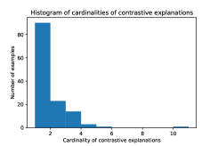
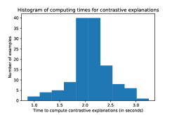
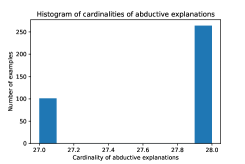
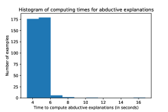
Figure 1: Explanation sizes and computing times on Loan Defaulter.

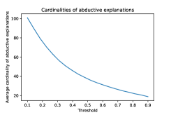
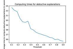
Figure 2: Explanation sizes and computing times on Blog Feedback.

We have implemented our greedy algorithms for computing cardinality-minimal explanations in Section 4.2 and assessed their practical suitability on well-known benchmark datasets commonly used to evaluate monotonic models. To the best of our knowledge, our implementation is the only one available for computing cardinality-minimal explanations and hence we could not find a suitable benchmark for comparison. All experiments were conducted using Google Colab with GPU.

Datasets.

The Blog Feedback Regression dataset Buza (2014) is a numeric dataset assembled from $37,279$ blog pages extracted from $1,200$ different sources. The objective is to predict the number of feedbacks that a blog page will receive in a given time window. The $276$ features include the number of links and feedbacks in the past, time and day of publication, discriminative bag of words, etc.

Loan Defaulter is a numeric dataset assembled from LendingClub (a large online loan marketplace). The objective is to predict if the applicant will repay the loan or default. The $28$ features include loans executed in the past, amount of the loan and instalments, applicant’s address and zip code, etc.

The features in both datasets are preprocessed and bounded between $0$ and $1$.

Methodology.

We trained monotonic FCN models on both datasets with PyTorch Paszke et al. (2019) using the mean-squared error loss for the Blog Feedback dataset and the binary cross entropy loss for the Loan Defaulter dataset. We trained the models with Adam Kingma and Ba (2014) for $10$ epochs, setting all negative weights to $0$ after each iteration of Adam to ensure monotonicity. We were able to reach a root mean-squared error (RMSE) of $0.175$ on the test set for the Blog Feedback regression (an acceptable performance given that the state-of-the-art is at $0.158$ Liu et al. (2020)) and reached an accuracy of $60\%$ on Loan Defaulter (state-of-the-art performance is $65.2\%$). Since the datasets are only partially-monotonic, we should not expect state-of-the-art performance with a fully-monotonic model; please note, however, that the objective of our experiments is not to improve on the state-of-the-art regression and classification metrics, but rather to show that cardinality-minimal explanations for the trained models can be efficiently computed.

Using the trained monotonic FCNs, we then computed cardinality-minimal abductive and contrastive explanations using the greedy algorithms in Section 4.2. Note that, although the models for Blog Feedback are trained for regression, our algorithms can still seamlessly be applied provided that we introduce a threshold. Indeed, given a FCN $\mathcal{N}:\Delta\mapsto\mathbb{R}$, an input vector $\mathbf{x}\in\Delta$ and a numeric threshold $t$ such that $\mathcal{N}(\mathbf{x})>t$ (respectively, $\leq t$), Algorithm 1 can be used to compute a cardinality-minimal subset $S$ such that $\mathcal{N}(\mathbf{x}^{S\mid\mathbf{x}^{\prime}})\leq t$ (respectively, $>t$) and a cardinality-minimal $S$ such that $\mathcal{N}(\mathbf{x}^{\overline{S}\mid\mathbf{z}})>t$ (respectively, $\leq t$) for all $\mathbf{z}\in\Delta$.

Results.

For Loan Defaulter, contrastive explanations took $1.5$s on average to compute and contained $1.8$ out of $28$ features on average; in turn, abductive explanations took $5s$ on average to compute and contained $27.6$ features on average. Note that contrastive explanations were much smaller than abductive explanations; this is not unexpected in a partially monotonic dataset since the condition required from abductive explanations requires the prediction to hold for all possible values of the features outside the explanation (a very strong condition). Figure 1 depicts the cardinalities and computation times for both types of explanations.

For the Blog Feedback Regression dataset, we varied the threshold between the lower bound and the upper bound of the targets and computed the average cardinality and computation time with respect to the threshold for both types of explanations. For contrastive explanations, the cardinality remained constant equal to 1: it was always possible to modify one feature and change the prediction. In the plots of Figure 2, we focused on abductive explanations and instances $\mathbf{x}$ such that $\mathcal{N}(\mathbf{x})\leq t$ and, as expected, we can see that the sizes of explanations decrease as the threshold increases.

7 Conclusion and Future Work

In this paper, we have studied the problem of computing cardinality-minimal contrastive and abductive explanations for the predictions of monotonic neural models. We have strengthened existing intractability results Barceló et al. (2020) to the context of monotonic fully-connected networks and proposed additional requirements to regain tractability.

Our results are of practical interest for the computation of explanations with formal guarantees in the context of monotonic or partially-monotonic tasks. Furthermore, from a theoretical perspective, our results not only strengthen existing intractability results, but to the best of our knowledge they also provide the first polytime algorithms for computing cardinality-minimal explanations in the context of neural models. Finally, our results also establish a novel connection between the theory of attribution methods and the theory of abductive and contrastive explanation methods, and have interesting implications for other related problems. We hope that our work will motivate further studies on the mathematical properties of explanation methods in Machine Learning.

References

- Adebayo et al. [2018] J. Adebayo, J. Gilmer, M. Muelly, I. Goodfellow, M. Hardt, and B. Kim. Sanity checks for saliency maps. In Advances in Neural Information Processing Systems, volume 31, 2018.
- Ancona et al. [2018] M. Ancona, E. Ceolini, C. Oztireli, and M. Gross. Towards better understanding of gradient-based attribution methods for deep neural networks. In International Conference on Learning Representations, 2018.
- Ancona et al. [2019] M. Ancona, C. Oztireli, and M. Gross. Explaining deep neural networks with a polynomial time algorithm for shapley values approximation. In Proceedings of the 36th International Conference on Machine Learning, volume 72, 2019.
- Aumann and Shapley [1974] R. J. Aumann and L.S. Shapley. Values of Non-Atomic Games. Princeton University Press, 1974.
- Bach et al. [2015] S. Bach, A. Binder, G. Montavon, F. Klauschen, K.-R. Müller, and W. Samek. On pixel-wise explanations for non-linear classifier decisions by layer-wise relevance propagation. PLoS ONE, 10, 2015.
- Bajaj et al. [2021] M. Bajaj, L. Chu, Z. Y. Xue, J. Pei, L. Wang, P. Cho-Ho Lam, and Y. Zhang. Robust counterfactual explanations on graph neural networks. In Advances in Neural Information Processing Systems, volume 34, 2021.
- Barceló et al. [2020] Pablo Barceló, Mikaël Monet, Jorge Pérez, and Bernardo Subercaseaux. Model interpretability through the lens of computational complexity. In Hugo Larochelle, Marc’Aurelio Ranzato, Raia Hadsell, Maria-Florina Balcan, and Hsuan-Tien Lin, editors, Proc. of NeurIPS, 2020.
- Blanc et al. [2021] Guy Blanc, Jane Lange, and Li-Yang Tan. Provably efficient, succinct, and precise explanations. In Marc’Aurelio Ranzato, Alina Beygelzimer, Yann N. Dauphin, Percy Liang, and Jennifer Wortman Vaughan, editors, Proc. of NeurIPS, pages 6129–6141, 2021.
- Blum and Rivest [1988] Avrim Blum and Ronald Rivest. Training a 3-node neural network is np-complete. In Advances in Neural Information Processing Systems, volume 1, 1988.
- Buza [2014] Krisztian Buza. Feedback prediction for blogs. In Data Analysis, Machine Learning and Knowledge Discovery, pages 145–152. Springer International Publishing, 2014.
- Cano et al. [2019] José Ramón Cano, Pedro Antonio Gutiérrez, Bartosz Krawczyk, Michal Wozniak, and Salvador García. Monotonic classification: An overview on algorithms, performance measures and data sets. Neurocomputing, 341:168–182, 2019.
- Chang et al. [2017] C.-H. Chang, E. Creager, A. Goldenberg, and D. Duvenaud. Interpreting neural network classifications with variational dropout saliency maps. In Advances in Neural Information Processing Systems, volume 30, 2017.
- Cucala et al. [2022a] D. J. T. Cucala, Bernardo Cuenca Grau, Egor V. Kostylev, and Boris Motik. Explainable GNN-based models over knowledge graphs. In International Conference on Learning Representations, 2022.
- Cucala et al. [2022b] David J. Tena Cucala, Bernardo Cuenca Grau, and Boris Motik. Faithful approaches to rule learning. In Gabriele Kern-Isberner, Gerhard Lakemeyer, and Thomas Meyer, editors, Proceedings of KR, 2022.
- Dabkowski and Gal [2017] P. Dabkowski and Y. Gal. Real time image saliency for black box classifiers. In Advances in Neural Information Processing Systems, volume 30, 2017.
- Darwiche [2020] Adnan Darwiche. Three modern roles for logic in AI. In Dan Suciu, Yufei Tao, and Zhewei Wei, editors, Proc. of PODS, pages 229–243. ACM, 2020.
- Dhurandhar et al. [2018] A. Dhurandhar, P.-Y. Chen, R. Luss, C.-C. Tu, P. Ting, K. Shanmugam, and P. Das. Explanations based on the missing: Towards contrastive ex- planations with pertinent negatives. Advances in Neural Information Processing Systems, 32, 2018.
- Friedman [2004] E. Friedman. Paths and consistency in additive cost sharing. Internation Journal of Game Theory, 32:501–518, 2004.
- Goodfellow et al. [2016] I. Goodfellow, Y. Bengio, and A. Courville. Deep Learning. MIT Press, 2016. http://www.deeplearningbook.org.
- Goyal et al. [2019] Y. Goyal, Z. Wu, J. Ernst, D. Batra, D. Parikh, and S. Lee. Counterfactual visual explanations. In Proceedings of the 36th International Conference on Machine Learning, volume 97, pages 2376–2384, 2019.
- Hannun et al. [2014] A. Hannun, C. Case, J. Casper, G. Diamos B. Catanzaro, E. Elsen, R. Prenger, S. Satheesh, S. Sengupta, A. Coates, and A. Y. Ng. Deep speech: Scaling up end-to-end speech recognition. arXiv preprint arXiv:1412.5567, 2014.
- Ignatiev et al. [2019] Alexey Ignatiev, Nina Narodytska, and João Marques-Silva. Abduction-based explanations for machine learning models. In Proc. of AAAI, pages 1511–1519. AAAI Press, 2019.
- Ignatiev et al. [2022] Alexey Ignatiev, Yacine Izza, Peter J. Stuckey, and João Marques-Silva. Using maxsat for efficient explanations of tree ensembles. In Proc. of AAAI, pages 3776–3785. AAAI Press, 2022.
- Izza and Marques-Silva [2021] Yacine Izza and João Marques-Silva. On explaining random forests with SAT. In Zhi-Hua Zhou, editor, Proc. of IJCAI, pages 2584–2591. ijcai.org, 2021.
- Jones [1997] L.K. Jones. The computational intractability of training sigmoidal neural networks. IEEE Transactions on Information Theory, 43(1):167–173, 1997.
- Judd [1988] Stephen Judd. On the complexity of loading shallow neural networks. Journal of Complexity, 4(3):177–192, 1988.
- Kazim and Koshiyama [2021] E. Kazim and A. S. Koshiyama. A high-level overview of ai ethics. Patterns, 2, 2021.
- Kingma and Ba [2014] Diederik P Kingma and Jimmy Ba. Adam: A method for stochastic optimization. arXiv preprint arXiv:1412.6980, 2014.
- Koh and Liang [2017] P. W. Koh and P. Liang. Understanding black-box predictions via influence functions. In Proceedings of the 34th International Conference on Machine Learning, volume 70, 2017.
- Krizhevsky et al. [2012] A. Krizhevsky, I. Sutskever, and G. E. Hinton. Imagenet classification with deepconvolutional neural networks. Advances in Neural Information Processing Systems, 25, 2012.
- Kumar et al. [2019] Abhinav Kumar, Thiago Serra, and Srikumar Ramalingam. Equivalent and approximate transformations of deep neural networks. CoRR, abs/1905.11428, 2019.
- LeCun et al. [2015] Y. LeCun, Y. Bengio, and G. Hinton. Deep learning. Nature, 521(7553):436–444, 2015.
- Li et al. [2018] O. Li, H. Liu, C. Chen, and C. Rudin. Deep learning for case-based reasoning through prototypes: A neural network that explains its predictions. Thirty-Second AAAI Conference on Artificial Intelligence, 2018.
- Liu et al. [2020] Xingchao Liu, Xing Han, Na Zhang, and Qiang Liu. Certified monotonic neural networks. In Advances in Neural Information Processing Systems, volume 33, pages 15427–15438, 2020.
- Lucic et al. [2022] A. Lucic, M. A. Ter Hoeve, G. Tolomei, M. De Rijke, and F. Silvestri. Cf-gnnexplainer: Counterfactual explanations for graph neural networks. In Proc. of IJCAI, volume 151, pages 4499–4511, 2022.
- Marques-Silva et al. [2021] João Marques-Silva, Thomas Gerspacher, Martin C. Cooper, Alexey Ignatiev, and Nina Narodytska. Explanations for monotonic classifiers. In Marina Meila and Tong Zhang, editors, Proc. of ICML 2021, volume 139, pages 7469–7479, 2021.
- Marques-Silva [2022] João Marques-Silva. Logic-based explainability in machine learning. CoRR, abs/2211.00541, 2022.
- Montavon et al. [2017] G. Montavon, S. Lapuschkin, A. Binder, W. Samek, and K.-R. Müller. Explaining nonlinear classification decisions with deep taylor decomposition. Pattern Recognition, 65:211–222, 2017.
- Paszke et al. [2019] A. Paszke, S. Gross, F. Massa, A. Lerer, J. Bradbury, G. Chanan, T. Killeen, Z. Lin, N. Gimelshein, L. Antiga, A. Desmaison, A. Kopf, E. Yang, Z. DeVito, M. Raison, A. Tejani, S. Chilamkurthy, B. Steiner, L. Fang, J. Bai, and S. Chintala. Pytorch: An imperative style, high-performance deep learning library. In Advances in Neural Information Processing Systems 32, pages 8024–8035. 2019.
- Schmidhuber [2015] J. Schmidhuber. Deep learning in neural networks: An overview. Neural networks, 61:85–117, 2015.
- Shapley [1953] L. Shapley. Contributions to the Theory of Games II. Princeton University Press, 1953.
- Shi et al. [2020] Weijia Shi, Andy Shih, Adnan Darwiche, and Arthur Choi. On tractable representations of binary neural networks. In Diego Calvanese, Esra Erdem, and Michael Thielscher, editors, Proc. of KR, pages 882–892, 2020.
- Shih et al. [2018] Andy Shih, Arthur Choi, and Adnan Darwiche. A symbolic approach to explaining bayesian network classifiers. In Jérôme Lang, editor, Proc. of IJCAI, pages 5103–5111. ijcai.org, 2018.
- Shrikumar et al. [2017] A. Shrikumar, P. Greenside, and P. Kundaje. Learning important features through propagating activation differences. In Proceedings of the 34th International Conference on Machine Learning, volume 70, pages 3145–3153. PMLR, 2017.
- Silver et al. [2016] D. Silver, A. Huang, C. J. Maddison, A. Guez, L. Sifre, G. van den Driessche, I. Antonoglou J. Schrittwieser, V. Panneershelvam, M. Lanctot, S. Dieleman, D. Grewe, J. Nham, N. Kalchbrenner, I. Sutskever, T. Lillicrap, M. Leach, K. Kavukcuoglu, T. Graepel, and D. Hassabis. Mastering the game of go with deep neural networks and tree search. Nature, 529, 2016.
- Simonyan et al. [2014] K. Simonyan, A. Vedaldi, and A. Zisserman. Deep inside convolutional networks: Visualising image classification models and saliency maps. In International Conference on Learning Representations, 2014.
- Sundararajan and Najmi [2020] M. Sundararajan and A. Najmi. The many shapley values for model explanation. In Proceedings of the 37th International Conference on Machine Learning, volume 119, pages 9269–9278. PMLR, 2020.
- Sundararajan et al. [2017] M. Sundararajan, A. Taly, and Q. Yan. Axiomatic attribution for deep networks. In Proceedings of the 34th International Conference on Machine Learning, volume 70, pages 3319–3328. PMLR, 2017.
- Wäldchen et al. [2021] Stephan Wäldchen, Jan MacDonald, Sascha Hauch, and Gitta Kutyniok. The computational complexity of understanding binary classifier decisions. J. Artif. Intell. Res., 70:351–387, 2021.
- Zhang et al. [2018] X. Zhang, A. Solar-Lezama, and R. Singh. Interpreting neural network judgments via minimal, stable, and symbolic corrections. In Advances in Neural Information Processing Systems, volume 31, 2018.