MCVD: Masked Conditional Video Diffusion for
Prediction, Generation, and Interpolation

Abstract

Video prediction is a challenging task. The quality of video frames from current state-of-the-art (SOTA) generative models tends to be poor and generalization beyond the training data is difficult. Furthermore, existing prediction frameworks are typically not capable of simultaneously handling other video-related tasks such as unconditional generation or interpolation. In this work, we devise a general-purpose framework called Masked Conditional Video Diffusion (MCVD) for all of these video synthesis tasks using a probabilistic conditional score-based denoising diffusion model, conditioned on past and/or future frames. We train the model in a manner where we randomly and independently mask all the past frames or all the future frames. This novel but straightforward setup allows us to train a single model that is capable of executing a broad range of video tasks, specifically: future/past prediction – when only future/past frames are masked; unconditional generation – when both past and future frames are masked; and interpolation – when neither past nor future frames are masked. Our experiments show that this approach can generate high-quality frames for diverse types of videos. Our MCVD models are built from simple non-recurrent 2D-convolutional architectures, conditioning on blocks of frames and generating blocks of frames. We generate videos of arbitrary lengths autoregressively in a block-wise manner. Our approach yields SOTA results across standard video prediction and interpolation benchmarks, with computation times for training models measured in 1-12 days using $\leq$ 4 GPUs.

Project page: https://mask-cond-video-diffusion.github.io

Code: https://mask-cond-video-diffusion.github.io/

1 Introduction

Predicting what one may visually perceive in the future is closely linked to the dynamics of objects and people. As such, this kind of prediction relates to many crucial human decision-making tasks ranging from making dinner to driving a car. If video models could generate full-fledged videos in pixel-level detail with plausible futures, agents could use them to make better decisions, especially safety-critical ones. Consider, for example, the task of driving a car in a tight situation at high speed. Having an accurate model of the future could mean the difference between damaging a car or something worse. We can obtain some intuitions about this scenario by examining the predictions of our model in Figure 1, where we condition on two frames and predict 28 frames into the future for a car driving around a corner. We can see that this is enough time for two different painted arrows to pass under the car. If one zooms in, one can inspect the relative positions of the arrow and the Mercedes hood ornament in the real versus predicted frames. Pixel-level models of trajectories, pedestrians, potholes, and debris on the road could one day improve the safety of vehicles.

Figure 1: Our approach generates high quality frames many steps into the future: Given two conditioning frames from the Cityscapes (Cordts et al., 2016) validation set (top left), we show 7 predicted future frames in row 2 below, then skip to frames 20-28, autoregressively predicted in row 4. Ground truth frames are shown in rows 1 and 3. Notice the initial large arrow advancing and passing under the car. In frame 20 (the far left of the 3rd and 4th row), the initially small and barely visible second arrow in the background of the conditioning frames has advanced into the foreground. Result generated by our MCVD concat model variant. Note that some Cityscapes videos contain brightness changes, which may explain the brightness change in this sample.

Although beneficial to decision making, video generation is an incredibly challenging problem; not only must high-quality frames be generated, but the changes over time must be plausible and ideally drawn from an accurate and potentially complex distribution over probable futures. Looking far in time is exceptionally hard given the exponential increase in possible futures. Generating video from scratch or unconditionally further compounds the problem because even the structure of the first frame must be synthesized. Also related to video generation are the simpler tasks of a) video prediction, predicting the future given the past, and b) interpolation, predicting the in-between given past and future. Yet, both problems remain challenging. Specialized tools exist to solve the various video tasks, but they rarely solve more than one task at a time.

Given the monumental task of general video generation, current approaches are still very limited despite the fact that many state of the art methods have hundreds of millions of parameters (Wu et al., 2021; Weissenborn et al., 2019; Villegas et al., 2019; Babaeizadeh et al., 2021). While industrial research is capable of looking at even larger models, current methods frequently underfit the data, leading to blurry videos, especially in the longer-term future and recent work has examined ways in improve parameter efficiency (Babaeizadeh et al., 2021). Our objective here is to devise a video generation approach that generates high-quality, time-consistent videos within our computation budget of $\leq$ 4 GPU) and computation times for training models $\leq$ two weeks. Fortunately, diffusion models for image synthesis have demonstrated wide success, which strongly motivated our use of this approach. Our qualitative results in Figure 1 also indicate that our particular approach does quite well at synthesizing frames in the longer-term future (i.e., frame 29 in the bottom right corner).

One family of diffusion models might be characterized as Denoising Diffusion Probabilistic Models (DDPMs) (Sohl-Dickstein et al., 2015; Ho et al., 2020; Dhariwal and Nichol, 2021), while another as Score-based Generative Models (SGMs) (Song and Ermon, 2019; Li et al., 2019; Song and Ermon, 2020; Jolicoeur-Martineau et al., 2021a). However, these approaches have effectively merged into a field we shall refer to as score-based diffusion models, which work by defining a stochastic process from data to noise and then reversing that process to go from noise to data. Their main benefits are that they generate very 1) high-quality and 2) diverse data samples. One of their drawbacks is that solving the reverse process is relatively slow, but there are ways to improve speed (Song et al., 2020; Jolicoeur-Martineau et al., 2021b; Salimans and Ho, 2022; Liu et al., 2022; Xiao et al., 2022). Given their massive success and attractive properties, we focus here on developing our framework using score-based diffusion models for video prediction, generation, and interpolation.

Our work makes the following contributions:

1. A conditional video diffusion approach for video prediction and interpolation that yields SOTA results.

2. A conditioning procedure based on masking past and/or future frames in a blockwise manner giving a single model the ability to solve multiple video tasks: future/past prediction, unconditional generation, and interpolation.

3. A sliding window blockwise autoregressive conditioning procedure to allow fast and coherent long-term generation (Figure 2).

4. A convolutional U-net neural architecture integrating recent developments with a conditional normalization technique we call SPAce-TIme-Adaptive Normalization (SPATIN) (Figure 3).

By conditioning on blocks of frames in the past and optionally blocks of frames even further in the future, we are able to better ensure that temporal dynamics are transferred across blocks of samples, i.e. our networks can learn implicit models of spatio-temporal dynamics to inform frame generation. Unlike many other approaches, we do not have explicit model components for spatio-temporal derivatives or optical flow or recurrent blocks.

2 Conditional Diffusion for Video

Let $\mathbf{x}_{0}\in\mathbb{R}^{d}$ be a sample from the data distribution $p_{\text{data}}$. A sample $\mathbf{x}_{0}$ can corrupted from $t=0$ to $t=T$ through the Forward Diffusion Process (FDP) with the following transition kernel:

$$q_{t}(\mathbf{x}_{t}|\mathbf{x}_{t-1})=\mathcal{N}(\mathbf{x}_{t};\sqrt{1-\beta_{t}}\mathbf{x}_{t-1},\beta_{t}\mathbf{I}),$$ (1)

Furthermore, $\mathbf{x}_{t}$ can be sampled directly from $\mathbf{x}_{0}$ using the following accumulated kernel:

$$q_{t}(\mathbf{x}_{t}|\mathbf{x}_{0})=\mathcal{N}(\mathbf{x}_{t};\sqrt{\bar{\alpha}_{t}}\mathbf{x}_{0},(1-\bar{\alpha}_{t})\mathbf{I})\implies{\mathbf{x}}_{t}=\sqrt{\bar{\alpha}_{t}}{\mathbf{x}}_{0}+\sqrt{1-\bar{\alpha}_{t}}{\bm{\epsilon}}$$ (2)

where $\bar{\alpha}_{t}=\prod_{s=1}^{t}(1-\beta_{s})$, and ${\bm{\epsilon}}\sim{\mathcal{N}}({\bm{0}},{\mathbf{I}})$.

Generating new samples can be done by reversing the FDP and solving the Reverse Diffusion Process (RDP) starting from Gaussian noise ${\mathbf{x}}_{T}$. It can be shown (Song et al. (2021); Ho et al. (2020)) that the RDP can be computed using the following transition kernel:

$$p_{t}(\mathbf{x}_{t-1}|\mathbf{x}_{t},\mathbf{x}_{0})=\mathcal{N}(\mathbf{x}_{t-1};\tilde{\bm{\mu}}_{t}(\mathbf{x}_{t},\mathbf{x}_{0}),\tilde{\beta}_{t}\mathbf{I}),$$

$$\text{where}\quad\tilde{\bm{\mu}}_{t}(\mathbf{x}_{t},\mathbf{x}_{0}) =\frac{\sqrt{\bar{\alpha}_{t-1}}\beta_{t}}{1-\bar{\alpha}_{t}}\mathbf{x}_{0}+\frac{\sqrt{\alpha_{t}}(1-\bar{\alpha}_{t-1})}{1-\bar{\alpha}_{t}}\mathbf{x}_{t}\quad\text{and}\quad\tilde{\beta}_{t}=\frac{1-\bar{\alpha}_{t-1}}{1-\bar{\alpha}_{t}}\beta_{t}$$ (3)

Since $\mathbf{x}_{0}$ given $\mathbf{x}_{t}$ is unknown, it can be estimated using eq. (2): $\hat{\mathbf{x}}_{0}=\big{(}{\mathbf{x}}_{t}-\sqrt{1-\bar{\alpha}_{t}}{\bm{\epsilon}}\big{)}/\sqrt{\bar{\alpha}_{t}}$, where ${\bm{\epsilon}}_{\theta}({\mathbf{x}}_{t}|t)$ estimates ${\bm{\epsilon}}$ using a time-conditional neural network parameterized by $\theta$. This allows us to reverse the process from noise to data. The loss function of the neural network is:

$$L(\theta)=\mathbb{E}_{t,\mathbf{x}_{0}\sim p_{\text{data}},{\bm{\epsilon}}\sim\mathcal{N}({\bm{0}},\mathbf{I})}\!\left[\left\|{\bm{\epsilon}}-{\bm{\epsilon}}_{\theta}(\sqrt{\bar{\alpha}_{t}}\mathbf{x}_{0}+\sqrt{1-\bar{\alpha}_{t}}{\bm{\epsilon}}\mid t)\right\|_{2}^{2}\right]$$ (4)

Note that estimating $\epsilon$ is equivalent to estimating a scaled version of the score function (i.e., the gradient of the log density) of the noisy data:

$$\nabla_{{\mathbf{x}}_{t}}\log q_{t}({\mathbf{x}}_{t}\mid{\mathbf{x}}_{0})=-\frac{1}{1-\bar{\alpha}_{t}}({\mathbf{x}}_{t}-\sqrt{\bar{\alpha}_{t}}{\mathbf{x}}_{0})=-\frac{1}{\sqrt{1-\bar{\alpha}_{t}}}{\bm{\epsilon}}$$ (5)

Thus, data generation through denoising depends on the score-function, and can be seen as noise-conditional score-based generation.

Score-based diffusion models can be straightforwardly adapted to video by considering the joint distribution of multiple continuous frames. While this is sufficient for unconditional video generation, other tasks such as video interpolation and prediction remain unsolved. A conditional video prediction model can be approximately derived from the unconditional model using imputation (Song et al., 2021); indeed, the contemporary work of Ho et al. (2022) attempts to use this technique; however, their approach is based on an approximate conditional model.

2.1 Video Prediction via Conditional Diffusion

We first propose to directly model the conditional distribution of video frames in the immediate future given past frames. Assume we have $p$ past frames ${\mathbf{p}}=\left\{{\mathbf{p}}^{i}\right\}_{i=1}^{p}$ and $k$ current frames in the immediate future $\mathbf{x}_{0}=\left\{\mathbf{x}_{0}^{i}\right\}_{i=1}^{k}$. We condition the above diffusion models on the past frames to predict the current frames:

$$L_{\text{vidpred}}(\theta)=\mathbb{E}_{t,[{\mathbf{p}},\mathbf{x}_{0}]\sim p_{\text{data}},{\bm{\epsilon}}\sim\mathcal{N}({\bm{0}},\mathbf{I})}\!\left[\left\|{\bm{\epsilon}}-{\bm{\epsilon}}_{\theta}(\sqrt{\bar{\alpha}_{t}}\mathbf{x}_{0}+\sqrt{1-\bar{\alpha}_{t}}{\bm{\epsilon}}\mid{\mathbf{p}},t)\right\|^{2}\right]$$ (6)

Given a model trained as above, video prediction for subsequent time steps can be achieved by blockwise autoregressively predicting current video frames conditioned on previously predicted frames (see Figure 2). We use variants of the network shown in Figure 3 to model ${\bm{\epsilon}}_{\theta}$ in Equation 6 here, and for Equation 7 and Equation 8 below.

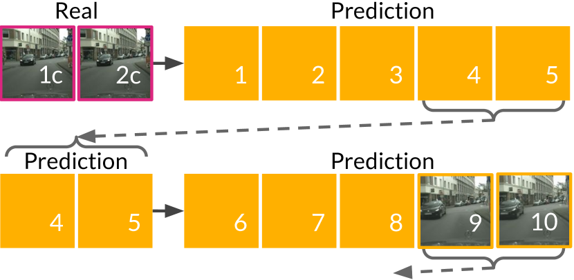
Figure 2: (Above) Blockwise autoregressive prediction with our model. (Right) shows this strategy where the top row and third row are ground truth, and the second and fourth rows show the blockwise autoregressively generated frames using our approach.

2.2 Video Prediction + Generation via Masked Conditional Diffusion

Our approach above allows video prediction, but not unconditional video generation. As a second approach, we extend the same framework to video generation by masking (zeroing-out) the past frames with probability $p_{\text{mask}}=\nicefrac{{1}}{{2}}$ using binary mask $m_{p}$. The network thus learns to predict the noise added without any past frames for context. Doing so means that we can perform conditional as well as unconditional frame generation, i.e., video prediction and generation with the same network. This leads to the following loss ($\mathcal{B}$ is the Bernouilli distribution):

$$L_{\text{vidgen}}(\theta)=\mathbb{E}_{t,[{\mathbf{p}},\mathbf{x}_{0}]\sim p_{\text{data}},{\bm{\epsilon}}\sim\mathcal{N}({\bm{0}},\mathbf{I}),m_{p}\sim\mathcal{B}(p_{\text{mask}})}\!\left[\left\|{\bm{\epsilon}}-{\bm{\epsilon}}_{\theta}(\sqrt{\bar{\alpha}_{t}}\mathbf{x}_{0}+\sqrt{1-\bar{\alpha}_{t}}{\bm{\epsilon}}\mid m_{p}{\mathbf{p}},t)\right\|^{2}\right]$$ (7)

We hypothesize that this dropout-like (Srivastava et al., 2014) approach will also serve as a form of regularization, improving the model’s ability to perform predictions conditioned on the past. We see positive evidence of this effect in our experiments – see the MCVD past-mask model variants in Sections 4 and 8 versus without past-masking. Note that random masking is used only during training.

2.3 Video Prediction + Generation + Interpolation via Masked Conditional Diffusion

We now have a design for video prediction and generation, but it still cannot perform video interpolation nor past prediction from the future. As a third and final approach, we show how to build a general model for solving all four video tasks. Assume we have $p$ past frames, $k$ current frames, and $f$ future frames ${\mathbf{f}}=\left\{{\mathbf{f}}^{i}\right\}_{i=1}^{f}$. We randomly mask the $p$ past frames with probability $p_{mask}=\nicefrac{{1}}{{2}}$, and similarly randomly mask the $f$ future frames with the same probability (but sampled separately). Thus, future or past prediction is when only future or past frames are masked. Unconditional generation is when both past and future frames are masked. Video interpolation is when neither past nor future frames are masked. The loss function for this general video machinery is:

$$L(\theta)=\mathbb{E}_{t,[{\mathbf{p}},{\mathbf{x}}_{0},{\mathbf{f}}]\sim p_{\text{data}},{\bm{\epsilon}}\sim\mathcal{N}({\bm{0}},\mathbf{I}),(m_{p},m_{f})\sim\mathcal{B}(p_{\text{mask}})}\!\left[\left\|{\bm{\epsilon}}-{\bm{\epsilon}}_{\theta}(\sqrt{\bar{\alpha}_{t}}\mathbf{x}_{0}+\sqrt{1-\bar{\alpha}_{t}}{\bm{\epsilon}}\mid m_{p}{\mathbf{p}},m_{f}{\mathbf{f}},t)\right\|^{2}\right]$$ (8)

2.4 Our Network Architecture

For our denoising network we use a U-net architecture (Ronneberger et al., 2015; Honari et al., 2016; Salimans et al., 2017) combining the improvements from Song et al. (2021) and Dhariwal and Nichol (2021). This architecture uses a mix of 2D convolutions (Fukushima and Miyake, 1982), multi-head self-attention (Cheng et al., 2016), and adaptive group-norm (Wu and He, 2018). We use positional encodings of the noise level ($t\in[0,1]$) and process it using a transformer style positional embedding:

$$\textbf{e}(t)=\left[\ldots,\cos\left(tc^{\frac{-2d}{D}}\right),\sin\left(tc^{\frac{-2d}{D}}\right),\ldots\right]^{\mathrm{T}},$$ (9)

where $d=1,\ldots,D/2$ , $D$ is the number of dimensions of the embedding, and $c=10000$. This embedding vector is passed through a fully connected layer, followed by an activation function and another fully connected layer. Each residual block has an fully connected layer that adapts the embedding to the correct dimensionality.

To provide $\mathbf{x}_{t}$, ${\mathbf{p}}$, and ${\mathbf{f}}$ to the network, we separately concatenate the past/future conditional frames and the noisy current frames in the channel dimension. The concatenated noisy current frames are directly passed as input to the network. Meanwhile, the concatenated conditional frames are passed through an embedding that influences the conditional normalization akin to SPatially-Adaptive (DE)normalization (SPADE) (Park et al., 2019); to account for the effect of time/motion, we call this approach SPAce-TIme-Adaptive Normalization (SPATIN).

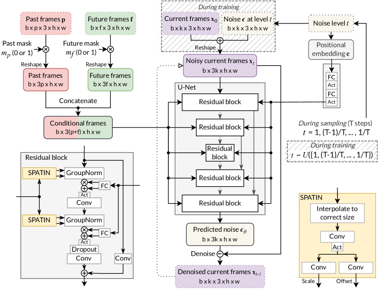
Figure 3: We give noisy current frames to a U-Net whose residual blocks receive conditional information from past/future frames and noise-level. The output is the predicted noise in the current frames, which we use to denoise the current frames. At test time, we start from pure noise.

In addition to SPATIN, we also try directly concatenating the conditional and noisy current frames together and passing them as the input. In our experiments below we show some results with SPATIN and some with concatenation (concat). For simple video prediction with Equation 6, we experimented with 3D convolutions and 3D attention However, this requires an exorbitant amount of memory, and we found no benefit in using 3D layers over 2D layers at the same memory (i.e., the biggest model that fits in 4 GPUs). Thus, we did not explore this idea further. We also tried and found no benefit from gamma noise (Nachmani et al., 2021), L1 loss, and F-PNDM sampling (Liu et al., 2022).

3 Related work

Score-based diffusion models have been used for image editing (Meng et al., 2022; Saharia et al., 2021; Nichol et al., 2021) and our approach to video generation might be viewed as an analogy to classical image inpainting, but in the temporal dimension. The GLIDE or Guided Language to Image Diffusion for Generation and Editing approach of  Nichol et al. (2021) uses CLIP-guided diffusion for image editing, while Denoising Diffusion Restoration Models (DDRM) Kawar et al. (2022) additionally condition on a corrupted image to restore the clean image. Adversarial variants of score-based diffusion models have been used to enhance quality (Jolicoeur-Martineau et al., 2021a) or speed (Xiao et al., 2022).

Contemporary work to our own such as that of  Ho et al. (2022) and Yang et al. (2022) also examine video generation using score-based diffusion models. However, the Video Diffusion Models (VDMs) work of Ho et al. (2022) approximates conditional distributions using a gradient method for conditional sampling from their unconditional model formulation. In contrast, our approach directly works with a conditional diffusion model, which we obtain through masked conditional training, thereby giving us the exact conditional distribution as well as the ability to generate unconditionally. Their experiments focus on: a) unconditional video generation, and b) text-conditioned video generation, whereas our work focuses primarily on predicting future video frames from the past, using our masked conditional generation framework. The Residual Video Diffusion (RVD) of  Yang et al. (2022) is only for video prediction, and it uses a residual formulation to generate frames autoregressively one at a time. Meanwhile, ours directly models the conditional frames to generate multiple frames in a block-wise autoregressive manner.

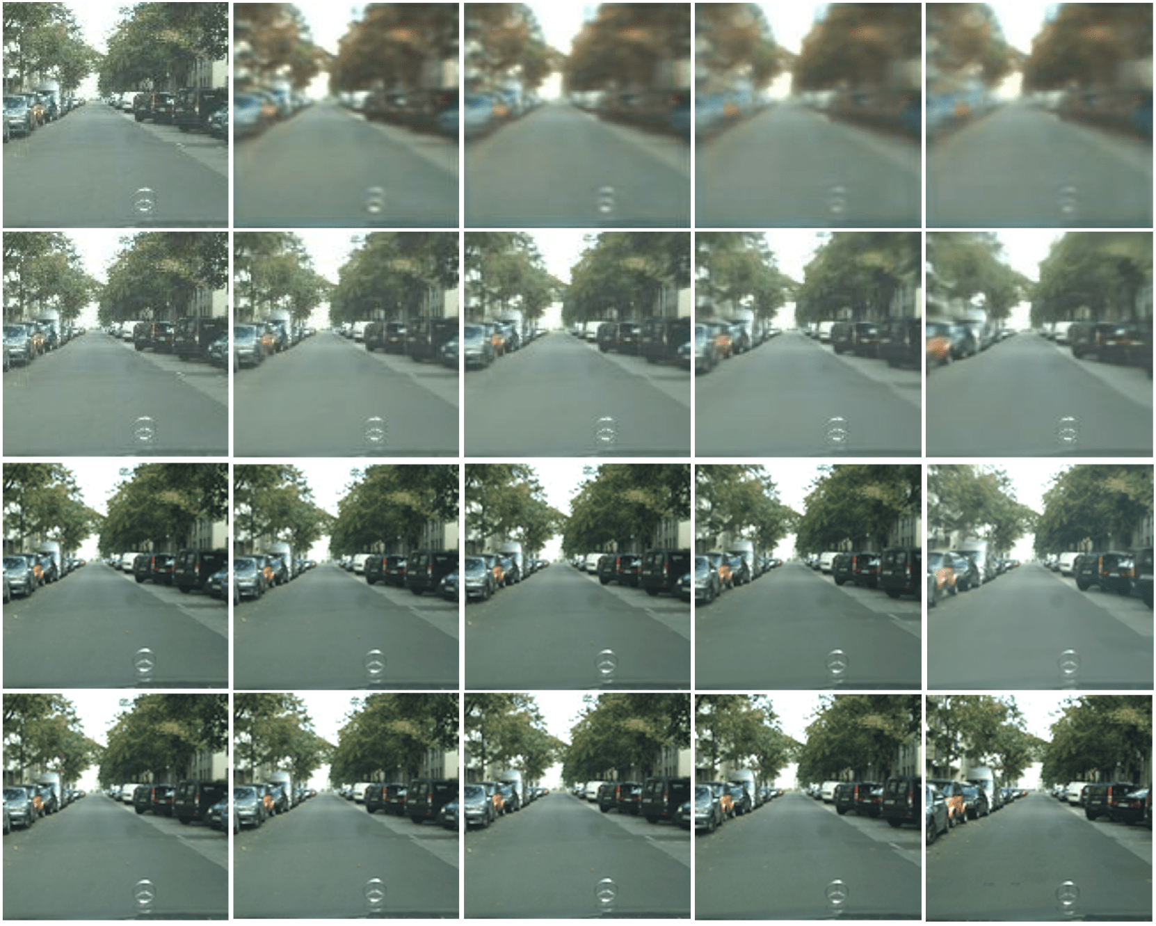
Figure 4: Comparing future prediction methods on Cityscapes: SVG-LP (Top Row), Hier-vRNNs (Second Row), Our Method (Third Row), Ground Truth (Bottom Row). Frame 2, a ground truth conditioning frame is shown in first column, followed by frames: 3, 5, 10 and 20 generated by each method vs the ground truth at the bottom.

Recurrent neural network (RNN) techniques were early candidates for modern deep neural architectures for video prediction and generation. Early work combined RNNs with a stochastic latent variable (SV2P) Babaeizadeh et al. (2018a) and was optimized by variational inference. The stochastic video generation (SVG) approach of Denton and Fergus (2018) learned both prior and a per time step latent variable model, which influences the dynamics of an LSTM at each step. The model is also trained in a manner similar to a variational autoencoder, i.e., it was another form of variational RNN (vRNN). To address the fact that vRNNs tend to lead to blurry results, Castrejón et al. (2019) (Hier-vRNN) increased the expressiveness of the latent distributions using a hierarchy of latent variables. We compare qualitative result of SVG and Hier-vRNN with the MCVD concat variant of our method in Figure 4. Other vRNN-based models include SAVP Lee et al. (2018), SRVP Franceschi et al. (2020), SLAMP Akan et al. (2021).

The well known Transformer paradigm (Vaswani et al., 2017) from natural language processing has also been explored for video. The Video-GPT work of Yan et al. (2021) applied an autoregressive GPT style (Brown et al., 2020) transformer to the codes produced from a VQ-VAE (Van Den Oord et al., 2017). The Video Transformer work of Weissenborn et al. (2019) models video using 3-D spatio-temporal volumes without linearizing positions in the volume. They examine local self-attention over small non-overlapping sub-volumes or 3D blocks. This is done partly to accelerate computations on TPU hardware. Their work also observed that the peak signal-to-noise ratio (PSNR) metric and the mean-structural similarity (SSIM) metrics (Wang et al., 2004) were developed for images, and have serious flaws when applied to videos. PSNR prefers blurry videos and SSIM does not correlate well to perceptual quality. Like them, we focus on the recently proposed Frechet Video Distance (FVD) (Unterthiner et al., 2018), computed over entire videos and which is sensitive to visual quality, temporal coherence, and diversity of samples. Rakhimov et al. (2020) (LVT) used transformers to predict the dynamics of video in latent space. Le Moing et al. (2021) (CCVS) also predict in latent space, that of an adversarially trained autoencoder, and also add a learnable optical flow module.

Generative Adversarial Network (GAN) based approaches to video generation have also been studied extensively. Vondrick et al. (2016) proposed an early GAN architecture for video, using a spatio-temporal CNN. Villegas et al. (2017) proposed a strategy for separating motion and content into different pathways of a convolutional LSTM based encoder-decoder RNN. Saito et al. (2017) (TGAN) predicted a sequence of latents using a temporal generator, and then the sequence of frames from those latents using an image generator. TGANv2 Saito et al. (2020) improved its memory efficiency. MoCoGAN Tulyakov et al. (2018) explored style and content separation, but within a CNN framework. Yushchenko et al. (2019) used the MoCoGAN framework by re-formulating the video prediction problem as a Markov Decision Process (MDP). FutureGAN Aigner and Körner (2018) used spatio-temporal 3D convolutions in an encoder decoder architecture, and elements of the progressive GAN Karras et al. (2018) approach to improve image quality. TS-GAN Munoz et al. (2021) facilitated information flow between consecutive frames. TriVD-GAN Luc et al. (2020) proposes a novel recurrent unit in the generator to handle more complex dynamics, while DIGAN Yu et al. (2022) uses implicit neural representations in the generator.

Video interpolation was the subject of a flurry of interest in the deep learning community a number of years ago (Niklaus et al., 2017; Jiang et al., 2018; Xue et al., 2019; Bao et al., 2019). However, these architectures tend to be fairly specialized to the interpolation task, involving optical flow or motion field modelling and computations. Frame interpolation is useful for video compression; therefore, many other lines of work have examined interpolation from a compression perspective. However, these architectures tend to be extremely specialized to the video compression task (Yang et al., 2020).

The Cutout approach of DeVries and Taylor (2017) has examined the idea of cutting out small continuous regions of an input image, such as small squares. Dropout (Srivastava et al., 2014) at the FeatureMap level was proposed and explored under the name of SpatialDropout in Tompson et al. (2015). Input Dropout (de Blois et al., 2020) has been examined in the context of dropping different channels of multi-modal input imagery, such as the dropping of the RGB channels or depth map channels during training, then using the model without one of the modalities during testing, e.g. in their work they drop the depth channel.

Regarding our block-autoregressive approach, previous video prediction models were typically either 1) non-recurrent: predicting all $n$ frames simultaneously with no way of adding more frames (most GAN-based methods), or 2) recurrent in nature, predicting 1 frame at a time in an autoregressive fashion. The benefit of the non-recurrent type is that you can generate videos faster than 1 frame at a time while allowing for generating as many frames as needed. The disadvantage is that it is slower than generating all frames at once, and takes up more memory and compute at each iteration. Our model finds a sweet spot in between in that it is block-autoregressive: generating $k<n$ frames at a time recurrently to finally obtain $n$ frames.

4 Experiments

We show the results of our video prediction experiments on test data that was never seen during training in Tables 1 - 3 for Stochastic Moving MNIST (SMMNIST) , KTH , BAIR , and Cityscapes respectively. We present unconditional generation results for BAIR in Table 4 and UCF-101  in Table 5, and interpolation results for SMMNIST, KTH, and BAIR in Table 6.

Datasets: We generate 128x128 images for Cityscapes and 64x64 images for the other datasets. See our Appendix and supplementary material for additional visual results. Our choice of datasets is in order of progressive difficulty: 1) SMMNIST: black-and-white digits; 2) KTH: grayscale single-humans; 3) BAIR: color, multiple objects, simple scene; 4) Cityscapes: color, natural complex natural driving scene; 5) UCF101: color, 101 categories of natural scenes. We process these datasets similarly to prior works. For Cityscapes, each video is center-cropped, then resized to $128\times 128$. For UCF101, each video clip is center-cropped at 240×240 and resized to 64×64, taking care to maintain the train-test splits.

Table 1: Video prediction results on SMMNIST ($64\times 64$) for 10 predicted frames conditioned on 5 past frames. We predicted 10 trajectories per real video, and report the average FVD and maximum SSIM, averaged across 256 test videos.

SMMNIST [5 $\rightarrow$ 10; trained on $k$]	$k$	FVD$\downarrow$	SSIM$\uparrow$
SVG (Denton and Fergus, 2018)	10	90.81	0.688
vRNN 1L (Castrejón et al., 2019)	10	63.81	0.763
Hier-vRNN (Castrejón et al., 2019)	10	57.17	0.760
MCVD concat (Ours)	5	25.63	0.786
MCVD spatin (Ours)	5	23.86	0.780

Unless otherwise specified, we set the mask probability to 0.5 when masking was used. For sampling, we report results using the sampling methods DDPM (Ho et al., 2020) or DDIM (Song et al., 2020) with only 100 sampling steps, though our models were trained with 1000, to make sampling faster. We observe that the metrics are generally better using DDPM than DDIM (except for UCF-101). Using 1000 sampling steps could yield better results.

Note that all our models are trained to predict only 4-5 current frames at a time, unlike other models that predict $\geq$10. We use these models to then autoregressively predict longer sequences for prediction or generation. This was done in order to fit the models in our GPU memory budget. Despite this disadvantage, we find that our MCVD models perform better than many previous SOTA methods.

Table 2: Video prediction results on KTH ($64\times 64$), predicting 30 and 40 frames using models trained to predict $k$ frames at a time. All models condition on 10 past frames, on 256 test videos.

KTH [10 $\rightarrow$ $pred$; trained on $k$]	$k$	$pred$	FVD$\downarrow$	PSNR$\uparrow$	SSIM$\uparrow$
SAVP (Lee et al., 2018)	10	30	374 $\pm$ 3	26.5	0.756
MCVD concat (Ours)	5	30	323 $\pm$ 3	27.5	0.835
SLAMP (Akan et al., 2021)	10	30	228 $\pm$ 5	29.4	0.865
SRVP (Franceschi et al., 2020)	10	30	222 $\pm$ 3	29.7	0.870
MCVD concat (Ours)	5	40	276.7	26.40	0.812
SAVP-VAE (Lee et al., 2018)	10	40	145.7	26.00	0.806
Grid-keypoints (Gao et al., 2021)	10	40	144.2	27.11	0.837

Metrics: As mentioned earlier, we primarily use the FVD metric for comparison across models as FVD measures both fidelity and diversity of the generated samples. Previous works compare Frechet Inception Distance (FID) (Heusel et al., 2017) and Inception Score (IS) (Salimans et al., 2016), adapted to videos by replacing the Inception network with a 3D-convolutional network that takes video input. FVD is computed similarly to FID, but using an I3D network trained on the huge video dataset Kinetics-400. We also report PSNR and SSIM.

Ablation studies: In section 4 we compare models that use concatenated raw pixels as input to U-Net blocks (concat) to SPATIN variants. We also compare no-masking to past-masking variants, i.e. models which are only trained predict the future vs. models which are regularized by being trained for prediction and unconditional generation. It can be seen that our model works across different choices of past frames and generates better quality for shorter videos. This is expected from models of this kind. Moreover, it can be seen that the model trained on the two tasks of Prediction and Generation (i.e., the models with past-mask) performs better than the model trained only on Prediction!

In addition, the appendix contains an ablation study in Table 8 on the different design choices: concat vs concat past-future-mask vs spatin vs spatin future-mask vs spatin past-future-mask. It can be seen that concat is, in general, better than spatin. It can also be seen that the past-future-mask variant, which is a general model capable of all three tasks, performs better at the individual tasks than the models trained only on the individual task. This was demonstrated in section 4 as well. This shows that the model gains very helpful insights while generalizing to all three tasks, which it does not while training only on the individual task.

We conducted preliminary experiments with a larger number of frames. Since the models with a larger number of frames were bigger, we could only run them for a shorter time with a smaller batch size than the smaller models. In general, we found that larger models did not substantially improve the results. We attribute this to the fact that using more frames means that the model should be given more capacity, but we could not increase it due to our computational budget constraints. We emphasize that our method works very well with fewer computational resources.

Examining these results we remark that we have SOTA performance for prediction on SMMNIST, BAIR and the challenging Cityscapes evaluation. Our Cityscapes model yields an FVD of 145.5, whereas the best previous result of which we are aware is 418. The quality of our Cityscapes results are illustrated visually in Figure 1 and Figure 2 and in the additional examples provided in our Appendix. While our completely unconditional generation results are strong, we note that when past masking is used to regularize future predicting models, we see clear performance gains in section 4. Finally, in Table 6 we see that our interpolation results are SOTA by a wide margin, across experiments on SMMNIST, KTH and BAIR – even compared to architectures much more specialized for interpolation.

It can be seen that our proposed method generates better quality videos, even though it was trained on a shorter number of frames than other methods. It can also be seen that training on multiple tasks using random masking improves the quality of generated frames than training on the individual tasks.

[h] Video prediction results on BAIR ($64\times 64$) conditioning on $p$ past frames and predicting $pred$ frames in the future, using models trained to predict $k$ frames at at time. BAIR ($64\times 64$) [past $p$ $\rightarrow$ $pred$ ; trained on $k$] $p$ $k$ $pred$ FVD$\downarrow$ PSNR$\uparrow$ SSIM$\uparrow$ LVT (Rakhimov et al., 2020) 1 15 15 125.8 – – DVD-GAN-FP (Clark et al., 2019) 1 15 15 109.8 – – MCVD spatin (Ours) 1 5 15 103.8 18.8 0.826 TrIVD-GAN-FP (Luc et al., 2020) 1 15 15 103.3 – – VideoGPT (Yan et al., 2021) 1 15 15 103.3 – – CCVS (Le Moing et al., 2021) 1 15 15 99.0 – – MCVD concat (Ours) 1 5 15 98.8 18.8 0.829 MCVD spatin past-mask (Ours) 1 5 15 96.5 18.8 0.828 MCVD concat past-mask (Ours) 1 5 15 95.6 18.8 0.832 Video Transformer (Weissenborn et al., 2019) 1 15 15 94-96^a – – FitVid (Babaeizadeh et al., 2021) 1 15 15 93.6 – – MCVD concat past-future-mask (Ours) 1 5 15 89.5 16.9 0.780 SAVP (Lee et al., 2018) 2 14 14 116.4 – – MCVD spatin (Ours) 2 5 14 94.1 19.1 0.836 MCVD spatin past-mask (Ours) 2 5 14 90.5 19.2 0.837 MCVD concat (Ours) 2 5 14 90.5 19.1 0.834 MCVD concat past-future-mask (Ours) 2 5 14 89.6 17.1 0.787 MCVD concat past-mask (Ours) 2 5 14 87.9 19.1 0.838 SAVP (Lee et al., 2018) 2 10 28 143.4 – 0.795 Hier-vRNN  (Castrejón et al., 2019) 2 10 28 143.4 – 0.822 MCVD spatin (Ours) 2 5 28 132.1 17.5 0.779 MCVD spatin past-mask (Ours) 2 5 28 127.9 17.7 0.789 MCVD concat (Ours) 2 5 28 120.6 17.6 0.785 MCVD concat past-mask (Ours) 2 5 28 119.0 17.7 0.797 MCVD concat past-future-mask (Ours) 2 5 28 118.4 16.2 0.745

• 94 on only the first frames, 96 on all subsequences of test frames

Table 3: Video prediction on Cityscapes ($128\times 128$) conditioning on 2 frames and predicting 28. SPATIN seems to produce a drift towards brighter images with a color balance shift in frames further from the start frame on Cityscapes, resulting in increased FVD for SPATIN than the CONCAT variant.

Cityscapes ($128\times 128$) [2 $\rightarrow$ 28; trained on $k$]	$k$	FVD$\downarrow$	LPIPS$\downarrow$	SSIM$\uparrow$
SVG-LP Denton and Fergus (2018)	10	1300.26	0.549 $\pm$ 0.06	0.574 $\pm$ 0.08
vRNN 1L  Castrejón et al. (2019)	10	682.08	0.304 $\pm$ 0.10	0.609 $\pm$ 0.11
Hier-vRNN  Castrejón et al. (2019)	10	567.51	0.264 $\pm$ 0.07	0.628 $\pm$ 0.10
GHVAE Wu et al. (2021)	10	418.00	0.193 $\pm$ 0.014	0.740 $\pm$ 0.04
MCVD spatin past-mask (Ours)	5	184.81	0.121 $\pm$ 0.05	0.720 $\pm$ 0.11
MCVD concat past-mask (Ours)	5	141.31	0.112 $\pm$ 0.05	0.690 $\pm$ 0.12

5 Conclusion

We have shown how to obtain SOTA video prediction and interpolation results with randomly masked conditional video diffusion models using a relatively simple architecture. We found that past-masking was able to improve performance across all model variants and configurations tested. We believe our approach may pave the way forward toward high quality larger-scale video generation.

Table 4: Unconditional generation of BAIR video frames.

BAIR ($64\times 64$) [0 $\rightarrow$ $pred$; trained on 5]	$pred$	FVD$\downarrow$
MCVD spatin past-mask (Ours)	16	267.8
MCVD concat past-mask (Ours)	16	228.5
MCVD spatin past-mask (Ours)	30	399.8
MCVD concat past-mask (Ours)	30	348.2

Table 5: Unconditional generation of UCF-101 video frames.

UCF-101 ($64\times 64$) [0 $\rightarrow$ 16; trained on $k$]	$k$	FVD$\downarrow$
MoCoGAN-MDP (Yushchenko et al., 2019)	16	1277.0
MCVD concat past-mask (Ours)	4	1228.3
TGANv2 (Saito et al., 2020)	16	1209.0
MCVD spatin past-mask (Ours)	4	1143.0
DIGAN (Yu et al., 2022)	16	655.0

Limitations. Videos generated by these models are still small compared to real movies, and they can still become blurry or inconsistent when the number of generated frames is very large. Our unconditional generation results on the highly diverse UCF-101 dataset are still far from perfect. More work is clearly needed to scale these models to larger datasets with more diversity and with longer duration video. As has been the case in many other settings, simply using larger models with many more parameters is a strategy that is likely to improve the quality and flexibility of these models – we were limited to 4 GPUs for our work here. There is also a need for faster sampling methods capable of maintaining quality over time.

Given our strong interpolation results, conditional diffusion models which generate skipped frames could make it possible to generate much longer, but consistent video through a strategy of first generating sparse distant frames in a block, followed by an interpolative diffusion step for the missing frames.

Table 6: Video Interpolation results (64 $\times$ 64). Given $p$ past + $f$ future frames $\rightarrow$ interpolate $k$ frames. Reporting average of the best metrics out of $n$ trajectories per test sample. $\downarrow\!(p\!+\!f)$ and $\uparrow\!k$ is harder. We used MCVD spatin past-mask for SMMNIST and KTH, and MCVD concat past-future-mask for BAIR. We also include results on SMMNIST for a "pure" model trained without any masking.

	SMMNIST ($64\times 64$)					KTH ($64\times 64$)					BAIR ($64\times 64$)
	$p\!\!+\!\!f$	$k$	$n$	PSNR$\uparrow$	SSIM$\uparrow$	$p\!\!+\!\!f$	$k$	$n$	PSNR$\uparrow$	SSIM$\uparrow$	$p\!\!+\!\!f$	$k$	$n$	PSNR$\uparrow$	SSIM$\uparrow$
SVG-LP Denton and Fergus (2018)	18	7	100	13.543	0.741	18	7	100	28.131	0.883	18	7	100	18.648	0.846
FSTN Lu et al. (2017)	18	7	100	14.730	0.765	18	7	100	29.431	0.899	18	7	100	19.908	0.850
SepConv Niklaus et al. (2017)	18	7	100	14.759	0.775	18	7	100	29.210	0.904	18	7	100	21.615	0.877
SuperSloMo Jiang et al. (2018)	18	7	100	13.387	0.749	18	7	100	28.756	0.893	–	–	–	–	–
SDVI full Xu et al. (2020)	18	7	100	16.025	0.842	18	7	100	29.190	0.901	18	7	100	21.432	0.880
SDVI Xu et al. (2020)	16	7	100	14.857	0.782	16	7	100	26.907	0.831	16	7	100	19.694	0.852
MCVD (Ours)	10	10	100	20.944	0.854	15	10	100	34.669	0.943	4	5	100	25.162	0.932
	10	5	10	27.693	0.941	15	10	10	34.068	0.942	4	5	10	23.408	0.914
	pure			18.385	0.802	10	5	10	35.611	0.963

Broader Impacts. High-quality video generation is potentially a powerful technology that could be used by malicious actors for applications such as creating fake video content. Our formulation focuses on capturing the distributions of real video sequences. High-quality video prediction could one day find use in applications such as autonomous vehicles, where the cost of errors could be high. Diffusion methods have shown great promise for covering the modes of real probability distributions. In this context, diffusion-based techniques for generative modelling may be a promising avenue for future research where the ability to capture modes properly is safety critical. Another potential point of impact is the amount of computational resources being spent for these applications involving the high fidelity and voluminous modality of video data. We emphasize the use of limited resources in achieving better or comparable results. Our submission provides evidence for more efficient computation involving fewer GPU hours spent in training time.

Checklist

1. For all authors…

   1. Do the main claims made in the abstract and introduction accurately reflect the paper’s contributions and scope? [Yes]

   2. Did you describe the limitations of your work? [Yes]

   3. Did you discuss any potential negative societal impacts of your work? [Yes]

   4. Have you read the ethics review guidelines and ensured that your paper conforms to them? [Yes]

2. If you are including theoretical results…

   1. Did you state the full set of assumptions of all theoretical results? [N/A]

   2. Did you include complete proofs of all theoretical results? [N/A]

3. If you ran experiments…

   1. Did you include the code, data, and instructions needed to reproduce the main experimental results (either in the supplemental material or as a URL)? [Yes] We will release the code with the supplementary

   2. Did you specify all the training details (e.g., data splits, hyperparameters, how they were chosen)? [Yes] We will provide this in the supplementary material, there was insufficient space to provide this in the main paper.

   3. Did you report error bars (e.g., with respect to the random seed after running experiments multiple times)? [Yes] Whenever possible.

   4. Did you include the total amount of compute and the type of resources used (e.g., type of GPUs, internal cluster, or cloud provider)? [Yes]

4. If you are using existing assets (e.g., code, data, models) or curating/releasing new assets…

   1. If your work uses existing assets, did you cite the creators? [Yes]

   2. Did you mention the license of the assets? [No] Readers can refer to the original references.

   3. Did you include any new assets either in the supplemental material or as a URL? [No] However we will link to a URL after peer review.

   4. Did you discuss whether and how consent was obtained from people whose data you’re using/curating? [N/A]

   5. Did you discuss whether the data you are using/curating contains personally identifiable information or offensive content? [N/A] We are using publicly available data collected by others.

5. If you used crowdsourcing or conducted research with human subjects…

   1. Did you include the full text of instructions given to participants and screenshots, if applicable? [N/A]

   2. Did you describe any potential participant risks, with links to Institutional Review Board (IRB) approvals, if applicable? [N/A]

   3. Did you include the estimated hourly wage paid to participants and the total amount spent on participant compensation? [N/A]

Appendix A Appendix

We provide some additional information regarding model size, memory requirements, batch size and computation times in Table 7. This is followed by additional results and visualizations for SMMNIST, KTH, BAIR, UCF-101 and Cityscapes.

For more sample videos, please visit https://mask-cond-video-diffusion.github.io For the code and pre-trained models, please visit https://github.com/voletiv/mcvd-pytorch. Our MCVD concat past-future-mask and past-mask results are of particular interest as they yield SOTA results across many benchmark configurations.

We tried to add the older FID and IS metrics (as opposed to the newer FVD metric which we used above) for UCF-101 as proposed in Saito et al. [2017], but we had difficulties integrating the chainer [Tokui et al., 2019] based implementation of these metrics into our PyTorch [Paszke et al., 2019] code base.

A.1 Computational requirements

Table 7: Compute used. "steps" indicates the checkpoint with the best approximate FVD, "GPU hours" is the total training time up to "steps".

Dataset,	params	CPU mem	batch	GPU	GPU mem	steps	GPU
model		(GB)	size		(GB)		hours
SMMNIST concat	27.9M	3.6	64	Tesla V100	14.5	700000	78.9
SMMNIST spatin	53.9M	3.3	64	RTX 8000	23.4	140000	39.7
KTH concat	62.8M	3.2	64	Tesla V100	21.5	400000	65.7
KTH spatin	367.6M	8.9	64	A100	145.9	340000	45.8
BAIR concat	251.2M	5.1	64	Tesla V100	76.5	450000	78.2
BAIR spatin	328.6M	9.2	64	A100	86.1	390000	50.0
Cityscapes concat	262.1M	6.2	64	Tesla V100	78.2	900000	192.83
Cityscapes spatin	579.1M	8.9	64	A100	101.2	650000	96.0
UCF concat	565.0M	8.9	64	Tesla V100	100.1	900000	183.95
UCF spatin	739.4M	8.9	64	A100	115.2	550000	79.5

A.2 Stochastic Moving MNIST

In Table 8 we provide results for more configurations of our proposed approach on the SMMNIST evaluation. In Figure 5 we provide some visual results for SMMNIST.

Table 8: Results on the SMMNIST evaluation, conditioned on 5 past frames, predicting 10 frames using models trained to predict 5 frames at a time.

SMMNIST [5 $\rightarrow$ 10; trained on 5]	FVD$\downarrow$	PSNR$\uparrow$	SSIM$\uparrow$	LPIPS$\downarrow$	MSE$\downarrow$
MCVD concat	25.63 $\pm$ 0.69	17.22	0.786	0.117	0.024
MCVD concat past-future-mask	20.77 $\pm$ 0.77	16.33	0.753	0.139	0.028
MCVD spatin	23.86 $\pm$ 0.67	17.07	0.785	0.129	0.025
MCVD spatin future-mask	44.14 $\pm$ 1.73	16.31	0.758	0.141	0.027
MCVD spatin past-future-mask	36.12 $\pm$ 0.63	16.15	0.748	0.146	0.027

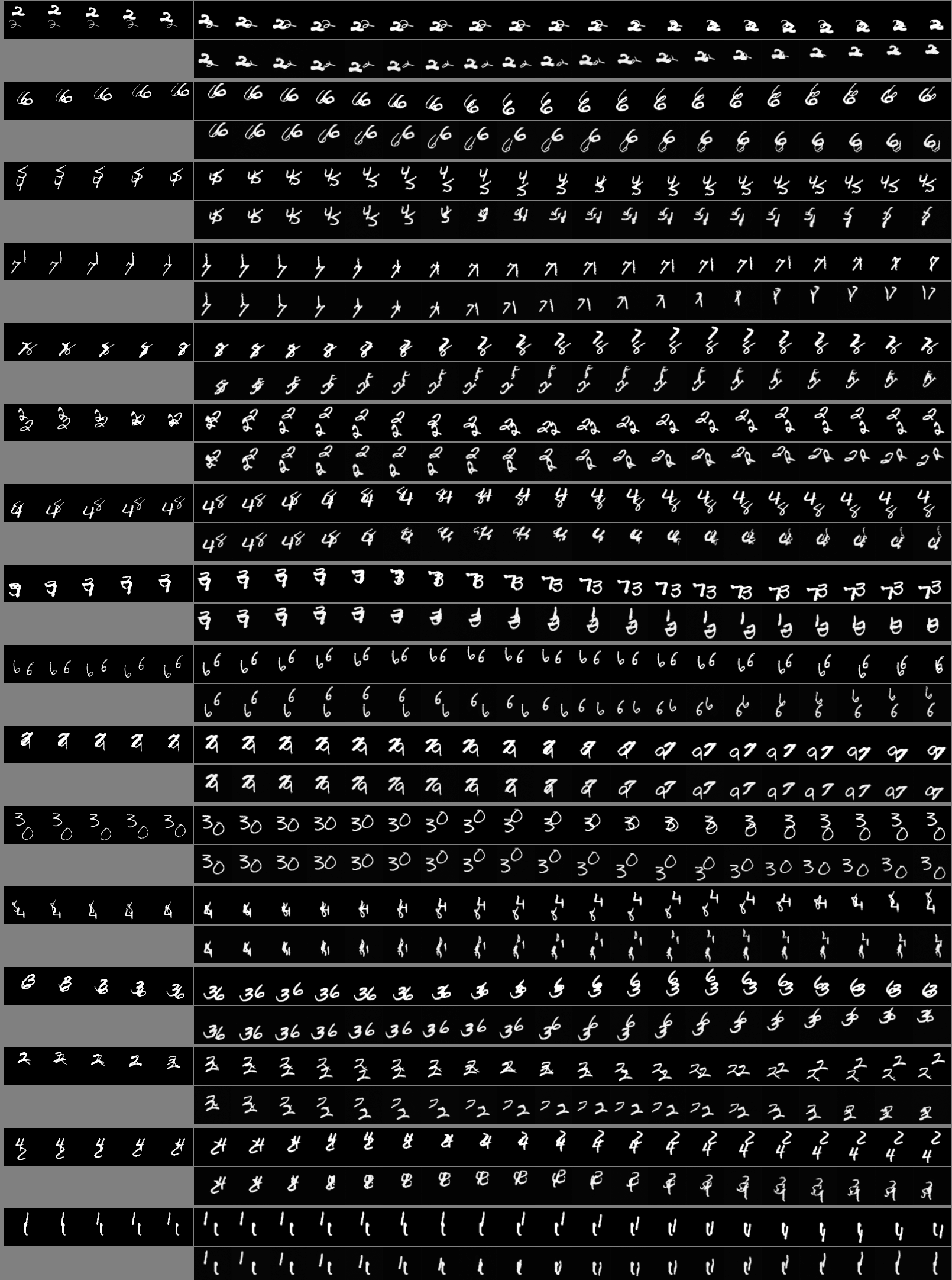
Figure 5: SMMNIST 5 $\to$ 10, trained on 5 (prediction). For each sample, top row is real ground truth, bottom is predicted by our MCVD model.

A.3 KTH

Table 9: Full table: Results on the KTH evaluation, predicting, 30 and 40 frames using models trained to predict $k$ frames at a time. All models condition on 10 past frames. SSIM numbers are updated from the main text after fixing a bug in the calculation.

KTH [10 $\rightarrow$ $pred$; trained on $k$]	$k$	$pred$	FVD$\downarrow$	PSNR$\uparrow$	SSIM$\uparrow$
SV2P [Babaeizadeh et al., 2018b]	10	30	636 $\pm$ 1	28.2	0.838
SVG-LP [Denton and Fergus, 2018]	10	30	377 $\pm$ 6	28.1	0.844
SAVP [Lee et al., 2018]	10	30	374 $\pm$ 3	26.5	0.756
MCVD spatin (Ours)	5	30	323 $\pm$ 3	27.5	0.835
MCVD concat past-future-mask (Ours)	5	30	294.9	24.3	0.746
SLAMP [Akan et al., 2021]	10	30	228 $\pm$ 5	29.4	0.865
SRVP [Franceschi et al., 2020]	10	30	222 $\pm$ 3	29.7	0.870
Struct-vRNN [Minderer et al., 2019]	10	40	395.0	24.29	0.766
MCVD concat past-future-mask (Ours)	5	40	368.4	23.48	0.720
MCVD spatin (Ours)	5	40	331.6 $\pm$ 5	26.40	0.744
MCVD concat (Ours)	5	40	276.6 $\pm$ 3	26.20	0.793
SV2P time-invariant [Babaeizadeh et al., 2018b]	10	40	253.5	25.70	0.772
SV2P time-variant  [Babaeizadeh et al., 2018b]	10	40	209.5	25.87	0.782
SAVP [Lee et al., 2018]	10	40	183.7	23.79	0.699
SVG-LP [Denton and Fergus, 2018]	10	40	157.9	23.91	0.800
SAVP-VAE [Lee et al., 2018]	10	40	145.7	26.00	0.806
Grid-keypoints [Gao et al., 2021]	10	40	144.2	27.11	0.837

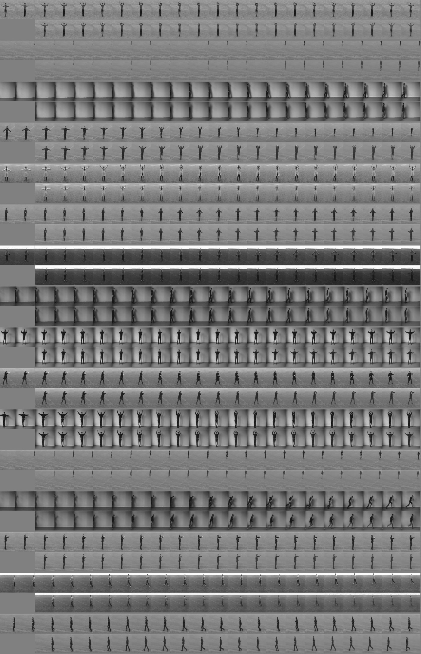
Figure 6: KTH 5 $\to$ 20, trained on 5 (prediction). For each sample, top row is real ground truth, bottom is predicted by our MCVD model. (We show only 2 conditional frames here)

A.4 BAIR

[h!] Full table: Results on the BAIR evaluation conditioning on $p$ past frames and predict pr frames in the future, using models trained to predict $k$ frames at at time. BAIR [past (p) $\rightarrow$ pred (pr) ; trained on k] p k pr FVD$\downarrow$ PSNR$\uparrow$ SSIM$\uparrow$ LVT [Rakhimov et al., 2020] 1 15 15 125.8 – – DVD-GAN-FP [Clark et al., 2019] 1 15 15 109.8 – – MCVD spatin (Ours) 1 5 15 103.8 18.8 0.826 TrIVD-GAN-FP [Luc et al., 2020] 1 15 15 103.3 – – VideoGPT [Yan et al., 2021] 1 15 15 103.3 – – CCVS [Le Moing et al., 2021] 1 15 15 99.0 – – MCVD concat (Ours) 1 5 15 98.8 18.8 0.829 MCVD spatin past-mask (Ours) 1 5 15 96.5 18.8 0.828 MCVD concat past-mask (Ours) 1 5 15 95.6 18.8 0.832 Video Transformer [Weissenborn et al., 2019] 1 15 15 94-96^a – – FitVid [Babaeizadeh et al., 2021] 1 15 15 93.6 – – MCVD concat past-future-mask (Ours) 1 5 15 89.5 16.9 0.780 SAVP [Lee et al., 2018] 2 14 14 116.4 – – MCVD spatin (Ours) 2 5 14 94.1 19.1 0.836 MCVD spatin past-mask (Ours) 2 5 14 90.5 19.2 0.837 MCVD concat (Ours) 2 5 14 90.5 19.1 0.834 MCVD concat past-future-mask (Ours) 2 5 14 89.6 17.1 0.787 MCVD concat past-mask (Ours) 2 5 14 87.9 19.1 0.838 SVG-LP [Akan et al., 2021] 2 10 28 256.6 – 0.816 SVG [Akan et al., 2021]. 2 12 28 255.0 18.95 0.8058 SLAMP [Akan et al., 2021] 2 10 28 245.0 19.7 0.818 SRVP [Franceschi et al., 2020] 2 12 28 162.0 19.6 0.820 WAM [Jin et al., 2020] 2 14 28 159.6 21.0 0.844 SAVP [Lee et al., 2018] 2 12 28 152.0 18.44 0.7887 vRNN 1L Castrejón et al. [2019] 2 10 28 149.2 – 0.829 SAVP [Lee et al., 2018] 2 10 28 143.4 – 0.795 Hier-vRNN  [Castrejón et al., 2019] 2 10 28 143.4 – 0.822 MCVD spatin (Ours) 2 5 28 132.1 17.5 0.779 MCVD spatin past-mask (Ours) 2 5 28 127.9 17.7 0.789 MCVD concat (Ours) 2 5 28 120.6 17.6 0.785 MCVD concat past-mask (Ours) 2 5 28 119.0 17.7 0.797 MCVD concat past-future-mask (Ours) 2 5 28 118.4 16.2 0.745

• 94 on only the first frames, 96 on all subsquences of test frames

Figure 7: BAIR 2 $\to$ 28, trained on 5 (prediction). For each sample, top row is real ground truth, bottom is predicted by our MCVD model.

A.5 UCF-101

Figure 8: UCF-101 4 $\to$ 16, trained on 4 (prediction). For each sample, top row is real ground truth, bottom is predicted by our MCVD model.

Figure 9: UCF-101 0 $\to$ 4 (generation)

A.6 Cityscapes

Here we provide some examples of future frame prediction for Cityscapes sequences conditioning on two frames and predicting the next 7 frames.

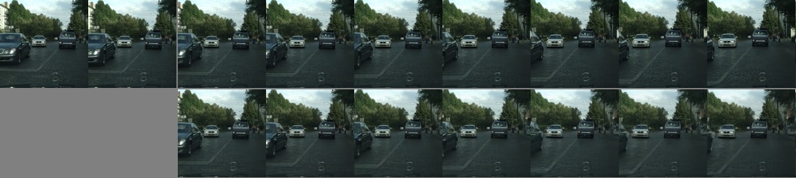
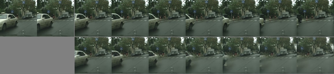
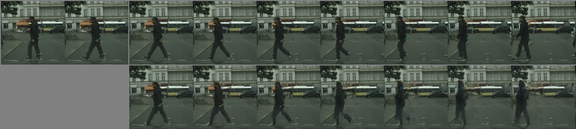
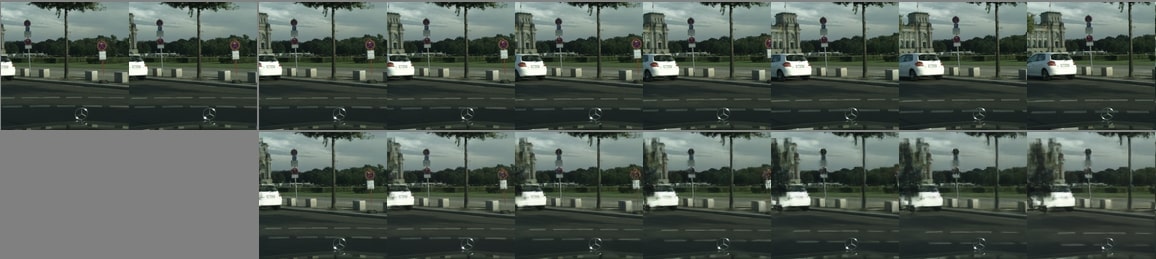
Figure 10: Cityscapes: 2 $\to$ 7, trained on 5 (prediction); Conditioning on the two frames in the top left corner of each block of two rows of images, we generate the next 7 frames. The top row is the true frames, bottom row contains the generated frames. We use the MCVD concat model variant.

For more examples, please visit https://mask-cond-video-diffusion.github.io

References

- Cordts et al. [2016] Marius Cordts, Mohamed Omran, Sebastian Ramos, Timo Rehfeld, Markus Enzweiler, Rodrigo Benenson, Uwe Franke, Stefan Roth, and Bernt Schiele. The cityscapes dataset for semantic urban scene understanding. In Proceedings of the IEEE conference on computer vision and pattern recognition, pages 3213–3223, 2016.
- Wu et al. [2021] Bohan Wu, Suraj Nair, Roberto Martin-Martin, Li Fei-Fei, and Chelsea Finn. Greedy hierarchical variational autoencoders for large-scale video prediction. In Proceedings of the IEEE/CVF Conference on Computer Vision and Pattern Recognition, pages 2318–2328, 2021.
- Weissenborn et al. [2019] Dirk Weissenborn, Oscar Täckström, and Jakob Uszkoreit. Scaling autoregressive video models. arXiv preprint arXiv:1906.02634, 2019.
- Villegas et al. [2019] Ruben Villegas, Arkanath Pathak, Harini Kannan, Dumitru Erhan, Quoc V Le, and Honglak Lee. High fidelity video prediction with large stochastic recurrent neural networks. Advances in Neural Information Processing Systems, 32, 2019.
- Babaeizadeh et al. [2021] Mohammad Babaeizadeh, Mohammad Taghi Saffar, Suraj Nair, Sergey Levine, Chelsea Finn, and Dumitru Erhan. Fitvid: Overfitting in pixel-level video prediction. arXiv preprint arXiv:2106.13195, 2021.
- Sohl-Dickstein et al. [2015] Jascha Sohl-Dickstein, Eric Weiss, Niru Maheswaranathan, and Surya Ganguli. Deep unsupervised learning using nonequilibrium thermodynamics. In International Conference on Machine Learning, pages 2256–2265. PMLR, 2015.
- Ho et al. [2020] Jonathan Ho, Ajay Jain, and Pieter Abbeel. Denoising diffusion probabilistic models. Advances in Neural Information Processing Systems, 2020.
- Dhariwal and Nichol [2021] Prafulla Dhariwal and Alexander Nichol. Diffusion models beat gans on image synthesis. Advances in Neural Information Processing Systems, 34, 2021.
- Song and Ermon [2019] Yang Song and Stefano Ermon. Generative modeling by estimating gradients of the data distribution. Advances in Neural Information Processing Systems, 2019.
- Li et al. [2019] Zengyi Li, Yubei Chen, and Friedrich T Sommer. Learning energy-based models in high-dimensional spaces with multi-scale denoising score matching. arXiv preprint arXiv:1910.07762, 2019.
- Song and Ermon [2020] Yang Song and Stefano Ermon. Improved techniques for training score-based generative models. Advances in Neural Information Processing Systems, 2020.
- Jolicoeur-Martineau et al. [2021a] Alexia Jolicoeur-Martineau, Rémi Piché-Taillefer, Rémi Tachet des Combes, and Ioannis Mitliagkas. Adversarial score matching and improved sampling for image generation. International Conference on Learning Representations, 2021a. URL arXivpreprintarXiv:2009.05475.
- Song et al. [2020] Jiaming Song, Chenlin Meng, and Stefano Ermon. Denoising diffusion implicit models. arXiv:2010.02502, October 2020. URL https://arxiv.org/abs/2010.02502.
- Jolicoeur-Martineau et al. [2021b] Alexia Jolicoeur-Martineau, Ke Li, Rémi Piché-Taillefer, Tal Kachman, and Ioannis Mitliagkas. Gotta go fast when generating data with score-based models. arXiv preprint arXiv:2105.14080, 2021b.
- Salimans and Ho [2022] Tim Salimans and Jonathan Ho. Progressive distillation for fast sampling of diffusion models. arXiv preprint arXiv:2202.00512, 2022.
- Liu et al. [2022] Luping Liu, Yi Ren, Zhijie Lin, and Zhou Zhao. Pseudo numerical methods for diffusion models on manifolds. arXiv preprint arXiv:2202.09778, 2022.
- Xiao et al. [2022] Zhisheng Xiao, Karsten Kreis, and Arash Vahdat. Tackling the generative learning trilemma with denoising diffusion GANs. In International Conference on Learning Representations (ICLR), 2022.
- Song et al. [2021] Yang Song, Jascha Sohl-Dickstein, Diederik P Kingma, Abhishek Kumar, Stefano Ermon, and Ben Poole. Score-based generative modeling through stochastic differential equations. International Conference on Learning Representations, 2021. URL arXivpreprintarXiv:2011.13456.
- Ho et al. [2022] Jonathan Ho, Tim Salimans, Alexey Gritsenko, William Chan, Mohammad Norouzi, and David J. Fleet. Video diffusion models, 2022. URL https://arxiv.org/abs/2204.03458.
- Srivastava et al. [2014] Nitish Srivastava, Geoffrey Hinton, Alex Krizhevsky, Ilya Sutskever, and Ruslan Salakhutdinov. Dropout: A simple way to prevent neural networks from overfitting. Journal of Machine Learning Research, 15(56):1929–1958, 2014.
- Ronneberger et al. [2015] Olaf Ronneberger, Philipp Fischer, and Thomas Brox. U-net: Convolutional networks for biomedical image segmentation. In International Conference on Medical image computing and computer-assisted intervention, pages 234–241. Springer, 2015.
- Honari et al. [2016] Sina Honari, Jason Yosinski, Pascal Vincent, and Christopher Pal. Recombinator networks: Learning coarse-to-fine feature aggregation. In Proceedings of the IEEE conference on computer vision and pattern recognition, pages 5743–5752, 2016.
- Salimans et al. [2017] Tim Salimans, Andrej Karpathy, Xi Chen, and Diederik P Kingma. Pixelcnn++: Improving the pixelcnn with discretized logistic mixture likelihood and other modifications. arXiv preprint arXiv:1701.05517, 2017.
- Fukushima and Miyake [1982] Kunihiko Fukushima and Sei Miyake. Neocognitron: A self-organizing neural network model for a mechanism of visual pattern recognition. In Competition and cooperation in neural nets, pages 267–285. Springer, 1982.
- Cheng et al. [2016] Jianpeng Cheng, Li Dong, and Mirella Lapata. Long short-term memory-networks for machine reading. arXiv preprint arXiv:1601.06733, 2016.
- Wu and He [2018] Yuxin Wu and Kaiming He. Group normalization. In Proceedings of the European conference on computer vision (ECCV), pages 3–19, 2018.
- Park et al. [2019] Taesung Park, Ming-Yu Liu, Ting-Chun Wang, and Jun-Yan Zhu. Semantic image synthesis with spatially-adaptive normalization. In Proceedings of the IEEE/CVF conference on computer vision and pattern recognition, pages 2337–2346, 2019.
- Nachmani et al. [2021] Eliya Nachmani, Robin San Roman, and Lior Wolf. Denoising diffusion gamma models. arXiv preprint arXiv:2110.05948, 2021.
- Meng et al. [2022] Chenlin Meng, Yutong He, Yang Song, Jiaming Song, Jiajun Wu, Jun-Yan Zhu, and Stefano Ermon. SDEdit: Guided image synthesis and editing with stochastic differential equations. In International Conference on Learning Representations, 2022.
- Saharia et al. [2021] Chitwan Saharia, William Chan, Huiwen Chang, Chris A Lee, Jonathan Ho, Tim Salimans, David J Fleet, and Mohammad Norouzi. Palette: Image-to-image diffusion models. arXiv preprint arXiv:2111.05826, 2021.
- Nichol et al. [2021] Alex Nichol, Prafulla Dhariwal, Aditya Ramesh, Pranav Shyam, Pamela Mishkin, Bob McGrew, Ilya Sutskever, and Mark Chen. Glide: Towards photorealistic image generation and editing with text-guided diffusion models. arXiv preprint arXiv:2112.10741, 2021.
- Kawar et al. [2022] Bahjat Kawar, Michael Elad, Stefano Ermon, and Jiaming Song. Denoising diffusion restoration models. arXiv preprint arXiv:2201.11793, 2022.
- Yang et al. [2022] Ruihan Yang, Prakhar Srivastava, and Stephan Mandt. Diffusion probabilistic modeling for video generation. arXiv preprint arXiv:2203.09481, 2022.
- Babaeizadeh et al. [2018a] Mohammad Babaeizadeh, Chelsea Finn, Dumitru Erhan, Roy H Campbell, and Sergey Levine. Stochastic variational video prediction. In International Conference on Learning Representations, 2018a.
- Denton and Fergus [2018] Emily Denton and Rob Fergus. Stochastic video generation with a learned prior. In Proceedings of the 35th International Conference on Machine Learning, pages 1174–1183, 2018.
- Castrejón et al. [2019] Lluís Castrejón, Nicolas Ballas, and Aaron C. Courville. Improved conditional vrnns for video prediction. ArXiv, abs/1904.12165, 2019.
- Lee et al. [2018] Alex X. Lee, Richard Zhang, Frederik Ebert, Pieter Abbeel, Chelsea Finn, and Sergey Levine. Stochastic adversarial video prediction. ArXiv, abs/1804.01523, 2018.
- Franceschi et al. [2020] Jean-Yves Franceschi, Edouard Delasalles, Mickaël Chen, Sylvain Lamprier, and Patrick Gallinari. Stochastic latent residual video prediction. In International Conference on Machine Learning, pages 3233–3246. PMLR, 2020.
- Akan et al. [2021] Adil Kaan Akan, Erkut Erdem, Aykut Erdem, and Fatma Güney. Slamp: Stochastic latent appearance and motion prediction. In Proceedings of the IEEE/CVF International Conference on Computer Vision, pages 14728–14737, 2021.
- Vaswani et al. [2017] Ashish Vaswani, Noam Shazeer, Niki Parmar, Jakob Uszkoreit, Llion Jones, Aidan N Gomez, Łukasz Kaiser, and Illia Polosukhin. Attention is all you need. In Adv. Neural Inform. Process. Syst., volume 30, 2017.
- Yan et al. [2021] Wilson Yan, Yunzhi Zhang, Pieter Abbeel, and Aravind Srinivas. Videogpt: Video generation using vq-vae and transformers. arXiv preprint arXiv:2104.10157, 2021.
- Brown et al. [2020] Tom Brown, Benjamin Mann, Nick Ryder, Melanie Subbiah, Jared D Kaplan, Prafulla Dhariwal, Arvind Neelakantan, Pranav Shyam, Girish Sastry, Amanda Askell, et al. Language models are few-shot learners. Adv. Neural Inform. Process. Syst., 33:1877–1901, 2020.
- Van Den Oord et al. [2017] Aaron Van Den Oord, Oriol Vinyals, et al. Neural discrete representation learning. Adv. Neural Inform. Process. Syst., 30, 2017.
- Wang et al. [2004] Zhou Wang, Alan C Bovik, Hamid R Sheikh, and Eero P Simoncelli. Image quality assessment: from error visibility to structural similarity. IEEE transactions on image processing, 13(4):600–612, 2004.
- Unterthiner et al. [2018] Thomas Unterthiner, Sjoerd van Steenkiste, Karol Kurach, Raphael Marinier, Marcin Michalski, and Sylvain Gelly. Towards accurate generative models of video: A new metric & challenges. arXiv preprint arXiv:1812.01717, 2018.
- Rakhimov et al. [2020] Ruslan Rakhimov, Denis Volkhonskiy, Alexey Artemov, Denis Zorin, and Evgeny Burnaev. Latent video transformer. arXiv preprint arXiv:2006.10704, 2020.
- Le Moing et al. [2021] Guillaume Le Moing, Jean Ponce, and Cordelia Schmid. Ccvs: Context-aware controllable video synthesis. Advances in Neural Information Processing Systems, 34, 2021.
- Vondrick et al. [2016] Carl Vondrick, Hamed Pirsiavash, and Antonio Torralba. Generating videos with scene dynamics. Advances in neural information processing systems, 29, 2016.
- Villegas et al. [2017] Ruben Villegas, Jimei Yang, Seunghoon Hong, Xunyu Lin, and Honglak Lee. Decomposing motion and content for natural video sequence prediction. In International Conference on Learning Representations, 2017.
- Saito et al. [2017] Masaki Saito, Eiichi Matsumoto, and Shunta Saito. Temporal generative adversarial nets with singular value clipping. In Proceedings of the IEEE international conference on computer vision, pages 2830–2839, 2017.
- Saito et al. [2020] Masaki Saito, Shunta Saito, Masanori Koyama, and Sosuke Kobayashi. Train sparsely, generate densely: Memory-efficient unsupervised training of high-resolution temporal gan. International Journal of Computer Vision, 128(10):2586–2606, 2020.
- Tulyakov et al. [2018] Sergey Tulyakov, Ming-Yu Liu, Xiaodong Yang, and Jan Kautz. Mocogan: Decomposing motion and content for video generation. In Proceedings of the IEEE conference on computer vision and pattern recognition, pages 1526–1535, 2018.
- Yushchenko et al. [2019] Vladyslav Yushchenko, Nikita Araslanov, and Stefan Roth. Markov decision process for video generation. In Proceedings of the IEEE/CVF International Conference on Computer Vision Workshops, pages 0–0, 2019.
- Aigner and Körner [2018] Sandra Aigner and Marco Körner. Futuregan: Anticipating the future frames of video sequences using spatio-temporal 3d convolutions in progressively growing gans. arXiv preprint arXiv:1810.01325, 2018.
- Karras et al. [2018] Tero Karras, Timo Aila, Samuli Laine, and Jaakko Lehtinen. Progressive growing of gans for improved quality, stability, and variation. In Int. Conf. Learn. Represent., 2018.
- Munoz et al. [2021] Andres Munoz, Mohammadreza Zolfaghari, Max Argus, and Thomas Brox. Temporal shift gan for large scale video generation. In Proceedings of the IEEE/CVF Winter Conference on Applications of Computer Vision, pages 3179–3188, 2021.
- Luc et al. [2020] Pauline Luc, Aidan Clark, Sander Dieleman, Diego de Las Casas, Yotam Doron, Albin Cassirer, and Karen Simonyan. Transformation-based adversarial video prediction on large-scale data. arXiv preprint arXiv:2003.04035, 2020.
- Yu et al. [2022] Sihyun Yu, Jihoon Tack, Sangwoo Mo, Hyunsu Kim, Junho Kim, Jung-Woo Ha, and Jinwoo Shin. Generating videos with dynamics-aware implicit generative adversarial networks. In International Conference on Learning Representations, 2022.
- Niklaus et al. [2017] Simon Niklaus, Long Mai, and Feng Liu. Video frame interpolation via adaptive convolution. In Proceedings of the IEEE Conference on Computer Vision and Pattern Recognition, pages 670–679, 2017.
- Jiang et al. [2018] Huaizu Jiang, Deqing Sun, Varun Jampani, Ming-Hsuan Yang, Erik Learned-Miller, and Jan Kautz. Super slomo: High quality estimation of multiple intermediate frames for video interpolation. In IEEE Conf. Comput. Vis. Pattern Recog., pages 9000–9008, 2018.
- Xue et al. [2019] Tianfan Xue, Baian Chen, Jiajun Wu, Donglai Wei, and William T Freeman. Video enhancement with task-oriented flow. Int. J. Comput. Vis., 127(8):1106–1125, 2019.
- Bao et al. [2019] Wenbo Bao, Wei-Sheng Lai, Chao Ma, Xiaoyun Zhang, Zhiyong Gao, and Ming-Hsuan Yang. Depth-aware video frame interpolation. In Proceedings of the IEEE/CVF Conference on Computer Vision and Pattern Recognition, pages 3703–3712, 2019.
- Yang et al. [2020] Ren Yang, Fabian Mentzer, Luc Van Gool, and Radu Timofte. Learning for video compression with recurrent auto-encoder and recurrent probability model. IEEE Journal of Selected Topics in Signal Processing, 15(2):388–401, 2020.
- DeVries and Taylor [2017] Terrance DeVries and Graham W Taylor. Improved regularization of convolutional neural networks with cutout. arXiv preprint arXiv:1708.04552, 2017.
- Tompson et al. [2015] Jonathan Tompson, Ross Goroshin, Arjun Jain, Yann LeCun, and Christoph Bregler. Efficient object localization using convolutional networks. In IEEE Conf. Comput. Vis. Pattern Recog., pages 648–656, 2015.
- de Blois et al. [2020] Sébastien de Blois, Mathieu Garon, Christian Gagné, and Jean-François Lalonde. Input dropout for spatially aligned modalities. In IEEE Int. Conf. Image Process., pages 733–737, 2020.
- Srivastava et al. [2015] Nitish Srivastava, Elman Mansimov, and Ruslan Salakhudinov. Unsupervised learning of video representations using lstms. In International conference on machine learning, pages 843–852. PMLR, 2015.
- Schuldt et al. [2004] Christian Schuldt, Ivan Laptev, and Barbara Caputo. Recognizing human actions: a local svm approach. In Proceedings of the 17th International Conference on Pattern Recognition, 2004. ICPR 2004., volume 3, pages 32–36. IEEE, 2004.
- Ebert et al. [2017] Frederik Ebert, Chelsea Finn, Alex X Lee, and Sergey Levine. Self-supervised visual planning with temporal skip connections. In CoRL, pages 344–356, 2017.
- Soomro et al. [2012] Khurram Soomro, Amir Roshan Zamir, and Mubarak Shah. Ucf101: A dataset of 101 human actions classes from videos in the wild. arXiv preprint arXiv:1212.0402, 2012.
- Gao et al. [2021] Xiaojie Gao, Yueming Jin, Qi Dou, Chi-Wing Fu, and Pheng-Ann Heng. Accurate grid keypoint learning for efficient video prediction. In 2021 IEEE/RSJ International Conference on Intelligent Robots and Systems (IROS), pages 5908–5915. IEEE, 2021.
- Heusel et al. [2017] Martin Heusel, Hubert Ramsauer, Thomas Unterthiner, Bernhard Nessler, and Sepp Hochreiter. Gans trained by a two time-scale update rule converge to a local nash equilibrium. In Advances in neural information processing systems, pages 6626–6637, 2017.
- Salimans et al. [2016] Tim Salimans, Ian Goodfellow, Wojciech Zaremba, Vicki Cheung, Alec Radford, Xi Chen, and Xi Chen. Improved techniques for training gans. In Advances in Neural Information Processing Systems, 2016.
- Clark et al. [2019] Aidan Clark, Jeff Donahue, and Karen Simonyan. Adversarial video generation on complex datasets. arXiv preprint arXiv:1907.06571, 2019.
- Lu et al. [2017] Chaochao Lu, Michael Hirsch, and Bernhard Scholkopf. Flexible spatio-temporal networks for video prediction. In Proceedings of the IEEE Conference on Computer Vision and Pattern Recognition, pages 6523–6531, 2017.
- Xu et al. [2020] Qiangeng Xu, Hanwang Zhang, Weiyue Wang, Peter Belhumeur, and Ulrich Neumann. Stochastic dynamics for video infilling. In Proceedings of the IEEE/CVF Winter Conference on Applications of Computer Vision, pages 2714–2723, 2020.
- Tokui et al. [2019] Seiya Tokui, Ryosuke Okuta, Takuya Akiba, Yusuke Niitani, Toru Ogawa, Shunta Saito, Shuji Suzuki, Kota Uenishi, Brian Vogel, and Hiroyuki Yamazaki Vincent. Chainer: A deep learning framework for accelerating the research cycle. In Proceedings of the 25th ACM SIGKDD International Conference on Knowledge Discovery & Data Mining, pages 2002–2011, 2019.
- Paszke et al. [2019] Adam Paszke, Sam Gross, Francisco Massa, Adam Lerer, James Bradbury, Gregory Chanan, Trevor Killeen, Zeming Lin, Natalia Gimelshein, Luca Antiga, et al. Pytorch: An imperative style, high-performance deep learning library. Advances in neural information processing systems, 32, 2019.
- Babaeizadeh et al. [2018b] Mohammad Babaeizadeh, Chelsea Finn, Dumitru Erhan, Roy H. Campbell, and Sergey Levine. Stochastic variational video prediction. International Conference on Learning Representations, 2018b.
- Minderer et al. [2019] Matthias Minderer, Chen Sun, Ruben Villegas, Forrester Cole, Kevin P Murphy, and Honglak Lee. Unsupervised learning of object structure and dynamics from videos. Advances in Neural Information Processing Systems, 32, 2019.
- Jin et al. [2020] Beibei Jin, Yu Hu, Qiankun Tang, Jingyu Niu, Zhiping Shi, Yinhe Han, and Xiaowei Li. Exploring spatial-temporal multi-frequency analysis for high-fidelity and temporal-consistency video prediction. In Proceedings of the IEEE/CVF Conference on Computer Vision and Pattern Recognition, pages 4554–4563, 2020.