Subset Node Anomaly Tracking
over Large Dynamic Graphs

Abstract.

Tracking a targeted subset of nodes in an evolving graph is important for many real-world applications. Existing methods typically focus on identifying anomalous edges or finding anomaly graph snapshots in a stream way. However, edge-oriented methods cannot quantify how individual nodes change over time while others need to maintain representations of the whole graph all the time, thus computationally inefficient.

This paper proposes DynAnom, an efficient framework to quantify the changes and localize per-node anomalies over large dynamic weighted-graphs. Thanks to recent advances in dynamic representation learning based on Personalized PageRank, DynAnom is 1) efficient: the time complexity is linear to the number of edge events and independent of node size of the input graph; 2) effective: DynAnom can successfully track topological changes reflecting real-world anomaly; 3) flexible: different type of anomaly score functions can be defined for various applications. Experiments demonstrate these properties on both benchmark graph datasets and a new large real-world dynamic graph. Specifically, an instantiation method based on DynAnom achieves the accuracy of 0.5425 compared with 0.2790, the best baseline, on the task of node-level anomaly localization while running 2.3 times faster than the baseline. We present a real-world case study and further demonstrate the usability of DynAnom for anomaly discovery over large-scale graphs.

1. Introduction

(a)

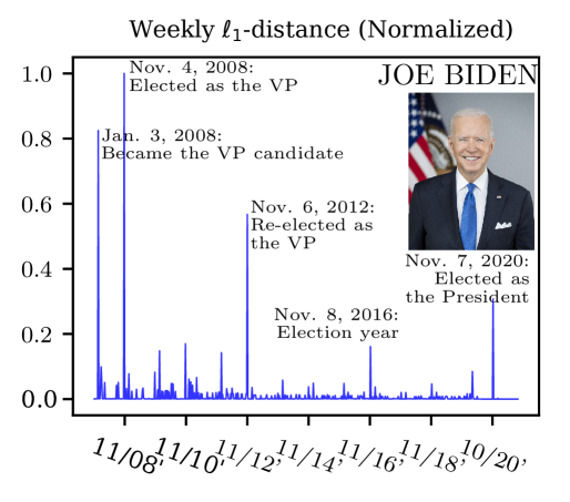
(b)

Figure 1. (a) Two consecutive snapshots $\mathcal{G}_{t}$ and $\mathcal{G}_{t+1}$ from a dynamic weighted-graph. The inserted edge $(u,v,1)$ further strengthens an existing relation, while edge $(u,k,1)$ builds a new link. (b) Anomaly tracking of Joe Biden over the Person Knowledge-Graph using our proposed DynAnom. We track Joe Biden on a weekly basis from 2007 to 2020, and calculate the $\ell_{1}$-distance between the representations on consecutive weeks. The detected peaks correlate well with significant changes in Biden’s life.

Analyzing the evolution of events in a large-scale dynamic network is important in many real-world applications. We are motivated by the following specific scenario:

Given a person-event interaction graph containing millions of nodes with several different types (e.g., person, event, location) with a stream of weekly updates over many years, how can we identify when specific individuals significantly changed their context?

The example in Fig. 1 shows our analysis as Joe Biden shifted his career from senator to vice president and finally to president. In each transition he relates with various intensity to other nodes across time. We seek to identify such transitions through analysis of these interaction frequencies and its inherent network structure. This task becomes challenging as the graph size and time horizon scale up. For example, the raw graph data used in Fig. 1 contains roughly 3.2 million nodes and 1196 weekly snapshots (each snapshot averages 4 million edges) of Person Graph from 2000 to 2022.

Despite the extensive literature (Akoglu et al., 2010; Yu et al., 2018; Bhatia et al., 2021a) on graph anomaly detection, previous work focuses on different problem definitions of anomaly. On the other hand, works (Yoon et al., 2019) on graph-level anomaly detection cannot identify individual node changes but only uncover the global changes in the overall graph structure. Most representative methods leverage tensor factorization (Chang et al., 2021) and graph sketching (Bhatia et al., 2021b), detecting the sudden dis/appearance of dense subgraphs. However, we argue that since most anomalies are locally incurred by a few anomalous nodes/edges, the global graph-level anomaly signal may overlook subtle local changes. Similarly, edge-level anomaly detection (Eswaran and Faloutsos, 2018) cannot identify node evolution when there is no direct edge event associated with that node. When Donald Trump became the president, his wife (Melania Trump) changed status to become First Lady, but no explicit edge changes connected her to other politicians except Trump. According to the edge-level anomaly detection, there is no evidence for Melania’s status change.

Node representation learning-based methods such as (Yu et al., 2018; Tsitsulin et al., 2021) could be helpful to identify anomaly change locally. However, it is impractical to directly apply these methods on large-scale dynamic settings due to 1) the low efficiency: re/training all node embeddings for snapshots is prohibitively expensive; 2) the missing alignment: node representations of each snapshot in the embedding space may not be inherently aligned, making the anomaly calculation difficult.

Inspired by the recent advances in local node representation methods (Postăvaru et al., 2020; Guo et al., 2021) for both static and dynamic graphs, we could efficiently calculate the node representations based on approximated Personalized PageRank vectors. These dynamic node representations are keys for capturing the evolution of a dynamic graph. One important observation is that the time complexity of calculating approximate PPV is $\mathcal{O}(\frac{1}{\alpha\epsilon})$ for per queried node, where $\alpha$ is PageRank (Page et al., 1999) teleport probability and $\epsilon$ is the approximation error tolerance. As the graph evolves, the per-node update complexity is $\mathcal{O}(\frac{|\Delta E|}{\epsilon})$, where $|\Delta E|$ is the total edge events. The other key observation is that the representation space is inherently consistent and aligned with each other, thus there is a meaningful metric space defined directly over the Euclidean space of every node representation across different times. Current local node representation method (Guo et al., 2021) only captures the node-level structural changes over unweighted graphs, which ignores the important interaction frequency information over the course of graph evolution. For example, in a communication graph, the inter-node interaction frequency is a strong signal, but the unweighted setting ignores such crucial feature. This undesirable characteristic makes the node representation becomes less expressive in weighted-graph.

In this paper, we generalize the local node representation method so that it is more expressive and supports dynamic weighted-graph, and the resolve the practical subset node anomaly tracking problem. We summarize our contributions as follows:

• We generalize dynamic forward push algorithm (Zhang et al., 2016) for calculating Personalized PageRank, making it suitable for weighted-graph anomaly tracking. The algorithm updates node representations per-edge event (i.e., weighted edge addition/deletion), and the per-node time complexity linear to edge events ($|\Delta E|$) and error parameter($\epsilon$) which is independent of the node size.

• We propose an efficient anomaly framework, namely DynAnom that can support both node and graph-level anomaly tracking, effectively localizing the period when a specified node significantly changed its context. Experiments demonstrate its superior performance over other baselines with the accuracy of 0.5425 compared with 0.2790, the baseline method meanwhile 2.3 times faster.

• A new large-scale real-world graph, as new resources for anomaly tracking: PERSON graph is constructed as a more interpretable resource, bringing more research opportunities for both algorithm benchmarking and real-world knowledge discovery. Furthermore, we conduct a case study of it, successfully capturing the career shifts of three public figures in U.S., showing the usability of DynAnom.

The rest paper is organized as follows: Section 2 reviews previous graph anomaly tracking methods. Section 3-4 describes the notation, preliminaries and problem formulation. We present our proposed framework – DynAnom in Section 5, and discuss experimental results in Section 6 Finally, we conclude and discuss future directions in Section 7. Our code and created datasets are accessible at https://github.com/zjlxgxz/DynAnom.

2. Related Work

We review three most common graph anomaly tasks over dynamic graphs, namely graph, edge and node-level anomaly.

Graph-level and edge-level anomaly.

Graph anomaly refers to sudden changes in the graph structure during its evolution, measuring the difference between consecutive graph snapshots (Aggarwal et al., 2011; Beutel et al., 2013; Eswaran and Faloutsos, 2018; Eswaran et al., 2018). Aggarwal et al. (2011) use a structural connectivity model to identify anomalous graph snapshots. Shin et al. (2017) apply incremental tensor factorization to spot dense connection formed in a short time. Yoon et al. (2019) use the first and second derivatives of the global PageRank Vectors as the anomaly signal, assuming that a normal graph stream will evolve smoothly. On the other hand, edge anomaly identifies unexpected edges as the graph evolves where anomalous edges adversarially link nodes in two sparsely connected components or abnormal edge weight changes (Ranshous et al., 2016; Eswaran and Faloutsos, 2018; Bhatia et al., 2020). Specifically, Eswaran and Faloutsos (2018) propose to use the approximated node-pair Personalized PageRank (PPR) score before and after the new edges being inserted. Most recently, Chang et al. (2021) estimate the interaction frequency between nodes, and incorporate the network structure into the parameterization of the frequency function. However, these methods cannot reveal the node local anomalous changes, and cannot identify the individual node changes for those without direct edge modification as we illustrated in introduction.

Node-level local anomaly.

Node anomaly measures the sudden changes in individual node’s connectivity, activity frequency or community shifts (Wang et al., 2015; Yu et al., 2018). Wang et al. (2015) uses hand-crafted features (e.g., node degree, centrality) which involve manual feature engineering processes. Recently, the dynamic node representation learning methods (Yu et al., 2018; Goyal et al., 2018; Zhou et al., 2018; Kumar et al., 2019; Lu et al., 2019; Sankar et al., 2020) were proposed. For example, a general strategy of them (Yu et al., 2018; Kumar et al., 2019) for adopting such dynamic embedding methods for anomaly detection is to incrementally update node representations and apply anomaly detection algorithms over the latent space. To measure the node changes over time, a comparable or aligned node representation is critical. Yu et al. (2018) uses auto-encoder and incremental random walk to update the node representations, then apply clustering algorithm to detect the node outliers in each snapshot. However, its disadvantage is that the embedding space is not aligned, making the algorithm only detects anomalies in each static snapshot. Even worse, it is inapplicable to large-scale graph because the fixed neural models is hard to expand without retraining. Similar approaches (Kumar et al., 2019) with more complicated deep learning structure were also studied. These existing methods are not suitable for the subset node anomaly tracking. Instead, our framework is inspired from recent advances in efficient local node representation algorithms (Zhang et al., 2016; Guo et al., 2017; Postăvaru et al., 2020; Guo et al., 2021), which is successful in handling subset node representations over large-scale graph.

3. Notations and Preliminaries

Notations.

Let $\mathcal{G}(\mathcal{V},\mathcal{E},\mathcal{W})$ be a directed weighted-graph where $\mathcal{V}$ is the set of nodes, $\mathcal{E}\subseteq\mathcal{V}\times\mathcal{V}$ is the set of edges, and $\mathcal{W}$ is corresponding edge weights of $\mathcal{E}$. For each node $v$, $\operatorname{Nei}(v)$ stands for out-neighbors of $v$. For all $v\in\mathcal{V}$, the generalized out-degree vector of $\mathcal{V}$ is $\bm{d}$ where $v$-th entry $d(v)\triangleq\sum_{u\in\operatorname{Nei}(v)}w_{(v,u)}$ and $w_{(v,u)}$ could be the weight of edge $(v,u)$ in graph $\mathcal{G}$. The generalized degree matrix is then denoted as $\bm{D}:=\operatorname{diag}(\bm{d})$ and the adjacency matrix is written as $\bm{A}$ with $\bm{A}(u,v)=w_{(u,v)}$.

3.1. PPR and Its Calculations

As a measure of the relative importance among nodes, PPR, a generalized version of original PageRank (Page et al., 1999), plays an important role in many graph mining tasks including tasks of anomaly tracking. Our framework is built on PPR. Specifically, the Personalized PageRank vector (PPV) of a node $s$ in $\mathcal{G}$ is defined as the following:

Definition 1 (Personalized PageRank Vector (PPV)).

Given a graph $\mathcal{G}(\mathcal{V},\mathcal{E},\mathcal{W})$ with $|\mathcal{V}|=n$ and $|\mathcal{E}|=m$. Define the lazy random walk transition matrix $\bm{P}\triangleq(1-\beta)\bm{D}^{-1}\bm{A}+\beta\bm{I}_{n}$, $\beta\in[0,1)$ where $\bm{D}$ is the generalized degree matrix and $\bm{A}$ is the adjacency matrix of $\mathcal{G}$. Given teleport probability $\alpha\in[0,1)$ and the source node $s$, the Personalized PageRank vector of $s$ is defined as:

(1) $$\bm{\pi}_{\alpha,s}=(1-\alpha)\bm{P}^{\top}\bm{\pi}_{\alpha,s}+\alpha\bm{1}_{s},$$

where the teleport probability $\alpha$ is a small constant (e.g. $\alpha=.15$), and $\bm{1}_{s}$ is an indicator vector of node $s$, that is, $s$-th entry is 1, 0 otherwise. We simply denote PPV of $s$ as $\bm{\pi}_{s}$.

Clearly, $\bm{\pi}_{s}$ can be calculated in a closed form, i.e., $\bm{\pi}_{s}=\alpha(\bm{I}_{n}-(1-\alpha)\bm{P}^{\top})^{-1}\bm{1}_{s}$ but with time complexity $\mathcal{O}(n^{3})$. The most commonly used method is Power Iteration (Page et al., 1999), which approximates $\bm{\pi}_{s}$ iteratively: $\bm{\pi}_{s}^{(t)}=(1-\alpha)\bm{P}^{\top}\bm{\pi}_{s}^{(t-1)}+\alpha\bm{1}_{s}$. After $t=\lceil\log_{1-\alpha}\epsilon\rceil$ iterations, one can achieve $\|\bm{\pi}_{s}-\bm{\pi}_{s}^{(t)}\|_{1}\leq\epsilon$. Hence, the overall time complexity of power iteration is $\mathcal{O}(m\log_{1-\alpha}\epsilon)$ with $\mathcal{O}(m)$ memory requirement. However, the per-iteration of the power iteration needs to access the whole graph which is time-consuming. Even worse, it is unclear how one can efficiently use power-iteration to obtain an updated $\bm{\pi}_{s}$ from $\mathcal{G}_{t}$ to $\mathcal{G}_{t+1}$. Other types of PPR can be found in (Wang et al., 2017; Wei et al., 2018; Wu et al., 2021) and references therein.

3.2. Dynamic Forward Push Algorithm

Instead, forward push algorithm (Andersen et al., 2006), a.k.a. the bookmark-coloring algorithm (Berkhin, 2006), approximates $\pi_{s}(v)$ locally via an approximate $p_{s}(v)$. The key idea is to maintain solution vector $\bm{p}_{s}$ and a residual vector $\bm{r}_{s}$ (at the initial $\bm{r}_{s}=\bm{1}_{s},\bm{p}_{s}=\bm{0}$). When the graph updates from $\mathcal{G}_{t}$ to $\mathcal{G}_{t+1}$, a variant forward push algorithm (Zhang et al., 2016) dynamically maintains $\bm{r}_{s}$ and $\bm{p}_{s}$. We generalize it to a weighted version of dynamic forward push to support dynamic updates on dynamic weighted-graph as presented in Algo. 1. At each local push iteration, it pushes large residuals to neighbors whenever these residuals are significant ($|r_{s}(u)|>\epsilon d(u)$). Compare with power-iteration, this operation avoids the access of whole graph hence speedup the calculations. Based on (Zhang et al., 2016), we consider a more general setting where the graph could be weighted-graph. Fortunately, this weighted version of DynamicForwardPush still has invariant property as presented in the following lemma.

Algorithm 1 DynamicForwardPush (Zhang et al., 2016)

1:Input: $\bm{p}_{s},\bm{r}_{s},\mathcal{G}_{t},\epsilon,\alpha$

2:while  exists $u$ such that $|r_{s}(u)|>\epsilon d(u)$ do

3:     $\textsc{Push}(u)$

4:return $(\bm{p}_{s},\bm{r}_{s})$

5:procedure Push($u$)

6:     $p_{s}(u)\mathrel{{+}{=}}\alpha r_{s}(u)$

7:     for $v\in\operatorname{Nei}(u)$ do

8:         $r_{s}(v)\mathrel{{+}{=}}\frac{(1-\alpha)r_{s}(u)w_{(u,v)}}{\sum_{v\in\operatorname{Nei}(u)}w_{(u,v)}}{\color[rgb]{0,0,1}}$      

9:     $r_{s}(u)=0$

Lemma 2 (PPR Invariant Property (Zhang et al., 2016)).

Suppose $\bm{\pi}_{s}$ is the PPV of node $s$ on graph $\mathcal{G}_{t}$. Let $\bm{p}_{s}$ and $\bm{\pi}_{s}$ be returned by the weighted version of DynamicForwardPush presented in Algo. 1. Then, we have the following invariant property.

(2) $$\pi_{s}(u) =p_{s}(u)+\sum_{x\in\mathcal{V}}r_{s}(x)\pi_{s}(x),\text{ for all }u\in\mathcal{V},\allowdisplaybreaks$$

(3) $$p_{s}(u)+\alpha r_{s}(u) =(1-\alpha)\sum_{x\in N^{in}(u)}\frac{w_{(u,x)}p_{s}(x)}{d(x)}+\alpha 1_{u=s},\allowdisplaybreaks$$

where $N^{in}(\cdot)$ is the in-neighbors, and $1_{u=s}=1$ if $u=s$, 0 otherwise.

From PPVs to node representations.

Obtained PPVs are not directly applicable to our anomaly tracking problem as operations on these $n$-dimensional vectors is time-consuming. To avoid this, we treat PPVs as the intriguing similarity matrix and project them into low-dimensional spaces using transformations such as SVD (Qiu et al., 2019), random projection (Zhang et al., 2018; Chen et al., 2019), matrix sketch(Tsitsulin et al., 2021), or hashing (Postăvaru et al., 2020) so that the original node similarity is well preserved by the low dimension node representations. We detail this in our main section.

4. Problem formulation

Before we present the subset node anomaly tracking problem. We first define the edge events in the dynamic graph model as the following: A set of edge events $\Delta E_{t}$ from $t$ to $t+1$ is a set of operations on edges, i.e., edge insertion, deletion or weight adjustment while the graph is updating from $\mathcal{G}_{t}$ to $\mathcal{G}_{t+1}$. Mathematically, $\Delta E_{t}\triangleq\{(u_{0},v_{0},\Delta w_{(u_{0},v_{0})},(u_{1},v_{1},\Delta w_{(u_{1},v_{1})})$, $\ldots,(u_{i},v_{i},\Delta w_{(u_{i},v_{i})})\}$ where each $\Delta w_{(u_{i},v_{i})}$ represents insertion (or weight increment) if it is positive, or deletion (decrement) if it is negative. Therefore, our dynamic graph model can be defined as a sequence of edge events. We state our formal problem definition as the following.

Definition 1 (Subset node Anomaly Tracking Problem).

Given a dynamic weighted-graph $\mathcal{G}_{t}=\langle\mathcal{V}_{t},\mathcal{E}_{t},\mathcal{W}_{t}\rangle,\forall t\in[0,T]$, consisting of initial snapshot $\mathcal{G}_{0}$ and the following T snapshots that have edge events $\Delta E_{t},|\Delta E_{t}|\geq 0$ (e.g., edge addition, deletion, weight adjustment from $t-1$ to $t$). We want to quantify the status change of a node $v$ in the targeted node subset $v\in\mathcal{S}\triangleq\{v_{0},v_{1},...,v_{k}\}$ from $\mathcal{G}_{t-1}$ to $\mathcal{G}_{t}$ with the anomaly measure function $f(\cdot,\cdot)$ so that the measurement is consistent to human judgement, or reflects the ground-truth of node status change if available. To illustrate this edge event process, Table 1 presents the process for better understanding.

Table 1. Illustration of subset node anomaly tracking problem. At each time $t$, node representations $\bm{x}_{i}^{t}$ are provided, and anomaly of node changes is quantified by $f(\bm{x}_{i}^{t-1},\bm{x}_{i}^{t}$), which is expected to correlated with the anomaly label if available.

Timestamp	0	1	2	3	…
Edge events	-	$\Delta E_{1}$	$\Delta E_{2}$	$\Delta E_{3}$	…
Snapshots	$G_{0}$	$G_{1}$	$G_{2}$	$G_{3}$	…
Score for $v_{i}\in\mathcal{S}$	-	$f(x_{i}^{0},x_{i}^{1})$	$f(x_{i}^{1},x_{i}^{2})$	$f(x_{i}^{2},x_{i}^{3})$	…
Label for $v_{i}\in\mathcal{S}$	-	Normal	Normal	Abnormal	…

5. The Proposed Framework

To localize the node anomaly across time, our idea is to incrementally obtain the PPVs as the node representation at each time, then design anomaly score function $f(\cdot,\cdot)$ to quantify the PPVs changes from time to time. This section presents our proposed framework DynAnom which has three components: 1) A provable dynamic PPV update strategy extending (Zhang et al., 2016) to weighted edge insertion/deletion; 2) Node level anomaly localization based on incremental PPVs; 3) Graph level anomaly detection based on approximation of global PageRank changes. We first present how local computation of PPVs can be generalized to dynamic weighted graphs, then present the unified framework for node/graph-level anomaly tracking, finally we analyze the complexity of an instantiation algorithm.

5.1. Maintenance of Dynamic PPVs

Multi-edges record the interaction frequency among nodes, and reflect the evolution of the network not only in topological structure, but also in the strength of communities. Previous works (Zhang et al., 2016; Guo et al., 2021) focus only on the structural changes over unweighted graph, ignoring the multi-edge cases. In a communication graph (e.g., Email graph), the disadvantage of such method is obvious: as more interactions/edges are observed, the graph becomes denser, or even turn out to be fully-connected in an extreme case. Afterwards, all the upcoming interactions will not change the node status since the ignorance of interaction frequency. This aforementioned scenario motivates us to generalize dynamic PPV maintenance to weighted graph, expanding its usability for more generic graphs and diverse applications. In order to incorporate edge weights into the dynamic forward push algorithm to obtain PPVs, we modify the original algorithm (Andersen et al., 2006; Zhang et al., 2016) by adding a weighted push mechanism as presented in Algo. 1. Specifically, for a specific node $v$, at each iteration of the push operation, we update its neighbor residual $r_{s}(v)$ as follows:

(4) $$r_{s}(v)\mathrel{{+}{=}}\frac{(1-\alpha)r_{s}(u)w_{(u,v)}}{\sum_{v\in\operatorname{Nei}(u)}w_{(u,v)}}.$$

The modified update of $r_{s}(v)$ in Equ. (4) efficiently approximate the PPR over static weighted graph with same time complexity as the original one. At time snapshot $\mathcal{G}_{t}$, the weight of each edge event $\Delta w_{(u,v)}$ could be either positive or negative, representing edge insertion or deletion) at time $t$ so that the target graph $\mathcal{G}_{t}$ updates to $\mathcal{G}_{t+1}$. However, this set of edge events will break up the invariant property shown in Lemma 2. To maintenance the invariant property on weighted graphs, we present the following Thm. 1, a generalized version from (Zhang et al., 2016). The key idea is to update $\bm{p}_{s},\bm{r}_{s}$ so that updated weights satisfy the invariant property. We present the theorem as follows:

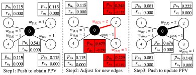
Figure 2. Illustration of the PPR adjustment over a weighted graph of five nodes. Step1: Apply Algo.1 to calculate the initial $p_{s},r_{s}$ where $s=v_{0},\alpha=0.15$ over the initial graph. Step2: After inserting new edges $(v_{0},v_{2},1),((v_{2},v_{3},1))$, the strength between $v_{0}$ and $v_{2}$ increases, and $v_{2}$ builds a new connection to $v_{3}$, which both break the invariant in Lemma 2. We adjust to recover the invariant by applying Theorem 1 in the red-colored blocks. Step3: We re-apply Algo.1 and update $p_{s}$ for better approximation error.

Generalized PPR update rules.

Figure 2 illustrates the dynamic maintenance of PPV over a weighted graph where two new edges are added, incurring edge weight increment between node 0 and 2, and new connection between node 2 and 3. Note that one only needs to have $\mathcal{O}(1)$ time to update $p_{s}(u),r_{s}(u)$, and $r_{s}(v)$ for each edge event. As proved, the total cost of $m$ edge events will be linearly dependent on, i.e., $\mathcal{O}(m)$. This efficient update procedure is much better than naive updates where one needs to calculate all quantities from scratch.

Theorem 1 (Generalized PPR update rules).

Given an edge event $(u,v,\Delta w_{(u,v)})$. We use the the following update rules

(5) $$p^{\prime}_{s}(u) =p_{s}(u)\frac{\sum_{v\in\operatorname{Nei}(u)}w_{(u,v)}+\Delta w_{(u,v)}}{\sum_{v\in\operatorname{Nei}(u)}w_{(u,v)}},$$

(6) $$r_{s}^{\prime}(u) =r_{s}(u)-\frac{\Delta w_{(u,v)}p_{s}(u)}{\alpha\sum_{v\in\operatorname{Nei}(u)}w_{(u,v)}},$$

(7) $$r_{s}^{\prime}(v) =r_{s}(v)+\frac{(1-\alpha)}{\alpha}\frac{\Delta w_{(u,v)}p_{s}(u)}{\sum_{v\in\operatorname{Nei}(u)}w_{(u,v)}}.$$

After applying a sequence of updating rules and using DynamicForwardPush algorithm, then $\bm{p}_{s}$ and $\bm{r}_{s}$ satisfy invariant property in Lemma 2 and accurately approximate PPV, as proved in Appendix A.

From dynamic PPVs to node representations.

The above theorem provides efficient rules to incrementally update PPVs for dynamic weighted graphs. To obtain dynamic node representation, two universal hash functions $h_{\operatorname{d}}$ and $h_{\operatorname{sgn}}$ are used (see details in (Postăvaru et al., 2020)). In the following section, we describe how to leverage PPVs as node representation for tracking node/graph-level anomaly.

5.2. Anomaly Tracking Framework: DynAnom

The key idea of our proposed framework is to measure the individual node anomaly in the embedding space based on Personalized PageRank (Postăvaru et al., 2020; Guo et al., 2021), and aggregate the individual anomaly scores to represent graph-level anomaly. By the fact that the PPV-based embedding space is aligned, we can directly measure the node anomaly by any distance function. We present our design as follows:

5.2.1. Node-level Anomaly Tracking

Since the inherently local characteristic of our proposed framework, we can efficiently measure the status of arbitrary nodes in two consecutive snapshots in an incrementally manner. Therefore, we could efficiently solve the problem defined in Def. 1 and localize where the anomaly actually happens by ranking the anomalous scores. To do this, the key ingredient is to measure node difference from $t-1$ to $t$ as $\delta_{s}^{t}=f(\bm{x}_{s}^{t-1},\bm{x}_{s}^{t})$ where $\bm{x}_{s}^{t}$ is the node representation of node $s$ at time $t$. Based on the above motivation, we first present the node-level anomaly detection algorithm DynAnom in Algo. 2 where the score function $f(\cdot,\cdot)$ is realized by $\ell_{1}$ norm in our experiments. There are three key steps: Step 1. calculating dynamic PPVs for all nodes in $S$ over $T$ snapshots (Line 3); Step 2. obtaining node representations of $S$ by local hash functions. Two universal hash functions are used in DynNodeRep (Line 5); Step 3. calculating node anomaly scores based on node representation $\bm{x}_{s}$ for all $s\in S$.

Noted that our design directly use the first-order difference ($\nabla x_{s}$) between two consecutive time. Although there are more complex design of $f(\cdot,\cdot)$ under this framework, such as, second-order measurement $\nabla^{2}x_{s}$ similar as in Yoon et al. (2019), clustering based anomaly detection (Yu et al., 2018), or supervised anomaly learning. We restrict our attention on the simplest form by setting $p=1\text{ or }2$ with the first-order measure. In our framework, the definition of anomaly score can be highly flexible for various applications.

Algorithm 2 $\textsc{DynAnom}(\mathcal{G}_{0},\Delta E_{1,\ldots,T},\mathcal{S},\epsilon,\alpha,p)$

1:Input: Initial graph $\mathcal{G}_{0}$, Edge events $\Delta E_{1,\ldots,T}$ , Subset target nodes $\mathcal{S}$, PPV quality $\epsilon$, teleport factor $\alpha$.

2://Step 1: Incrementally calculate PPVs

3:$\bm{p}_{s\in\mathcal{S}}=\textsc{IncrementPush}(\mathcal{G}_{0},\Delta E_{1,\ldots,T},S,\epsilon,\alpha)$

4://Step 2: Obtain node representations in target set $\mathcal{S}$

5:$\bm{x}_{s\in\mathcal{S}}=\textsc{DynNodeRep}(p_{s}^{0},...,P_{s}^{T})$

6://Step 3: Calculate node anomaly for all nodes in $\mathcal{S}$

7:for $s\in S,t\in[1,T]$ do

8:     $\delta_{s}^{t}=f(x_{s}^{t-1},x_{s}^{t})=\left(\sum_{i}\left|x_{s}^{t}(i)-x_{s}^{t-1}(i)\right|^{p}\right)^{1/p}$

9:return $\bm{\delta}_{s}=[\delta_{s}^{1},\delta_{s}^{2},\ldots,\delta_{s}^{T}],\forall s\in S$

10:procedure IncrementPush($\mathcal{G}_{0},\Delta E_{1,\ldots,T},\mathcal{S},\epsilon,\alpha$)

11:     $t=0$

12:     for $s\in\mathcal{S}:=\{v_{1},v_{2},\ldots,v_{k}\}$ do

13:         $p_{s}^{t}=\bm{0},\quad r_{s}^{t}=1_{s}$

14:         $p_{s}^{t},r_{s}^{t}=$DynamicForwardPush$(\mathcal{G}^{0},s,p_{s}^{t},r_{s}^{t},\epsilon,\alpha)$      

15:     for $t\in[1,T]$ do

16:         for $s\in\mathcal{S}$ do

17:              for $(u,v,\Delta w_{(u,v)})\in\Delta E_{t}$ do

18:                  update $p_{s}^{t}(u),r_{s}^{t}(u),r_{s}^{t}(v)$ uses rules in Thm. 1.               

19:              $p_{s}^{t},r_{s}^{t}=$DynamicForwardPush$(\mathcal{G}^{0},s,p_{s}^{t},r_{s}^{t},\epsilon,\alpha)$          

20:         $\mathcal{G}_{t}+=(u,v,\Delta w_{(u,v)})$      

21:     return $\bm{p}_{s}=[p_{s}^{0},...,p_{s}^{T}],\forall s\in S$

22:procedure DynNodeRep($\bm{p}_{s}^{0},\ldots,\bm{p}_{s}^{T}$)

23:     $\epsilon_{c}=\textsc{min}(\frac{1}{|\mathcal{V}|},\text{1e-5}),dim=1024$

24:     for $t\in[1,T)$ do

25:         for $i\in\cup_{t^{\prime}\in\{t,t-1\}}\textsc{supp}(p_{s}^{t^{\prime}})$ do:

26:              $p_{s}^{t-1}(i)=0$ if $p_{s}^{t-1}(i)\leq\epsilon_{c}$

27:              $p_{s}^{t}(i)=0$ if $p_{s}^{t}(i)\leq\epsilon_{c}$          

28:         $x_{s}^{t}=\textsc{ReduceDim}(\frac{p_{s}^{t}}{\|p_{s}^{t}\|_{1}},dim)$

29:         $x_{s}^{t-1}=\textsc{ReduceDim}(\frac{p_{s}^{t-1}}{\|p_{s}^{t-1}\|_{1}},dim)$

30:         return $\bm{x}_{s}=[x_{s}^{0},...,x_{s}^{T}],\forall s\in S$      

31:procedure ReduceDim($x,dim$)

32:     // Hash function $h_{dim}(i):\mathbb{N}\to[dim]$

33:     // Hash function $h_{\operatorname{sgn}}(i):\mathbb{N}\to\{\pm 1\}$

34:     if $\textsc{dim}(x)\leq dim$ then

35:         return $x$

36:     else

37:         $\bar{x}=\bm{0}\in\mathcal{R}^{dim}$

38:         for $i\in\textsc{Supp}(x)$ do

39:              $\bar{x}(h_{dim}(i))\mathrel{{+}{=}}h_{\operatorname{sgn}}(i)\log\left(x(i)\right)$          

40:         return $\frac{\bar{x}}{\|\bar{x}\|_{1}}$      

5.2.2. Graph-level Anomaly Tracking

Based on the node-level anomaly score proposed in Algo. 2, we propose the graph-level anomaly. The key property we used for graph-level anomaly tracking is the linear relation property of PPV. More specifically, let $\bm{\pi}$ be the PageRank vector. We note that the PPR vector is linear to personalized vector $\bm{\pi}_{s}$. Therefore, global PageRank could be calculated by the weighted average of single source PPVs.

(8) $$\bm{\pi}=\alpha\frac{\bm{\vec{}}1}{|\mathcal{V}|}\sum_{i=0}^{\infty}(1-\alpha)^{i}\bm{P}^{i}=\sum_{s\in\mathcal{V}}\frac{1_{s}}{|\mathcal{V}|}\bm{\pi}_{s}=\frac{1}{|\mathcal{V}|}\sum_{s\in\mathcal{V}}\bm{\pi}_{s},\allowdisplaybreaks$$

From the above linear equality, we formulate the global PPV, denoted as $\pi_{,g}$,as the linear combination of single-source PPVs as following:

(9) $$\bm{\pi}_{g}=\sum_{s\in\mathcal{V}}\gamma_{s}\pi_{s},\gamma_{s}=\frac{d(s)}{m},m=\sum_{i\in\mathcal{V}}d(i)\allowdisplaybreaks$$

In order to capture the graph-level anomaly, we use the similar heuristic weights (Yoon et al., 2019) $\gamma_{s}=\frac{d(s)}{m}$, which implies that $\bm{\pi}_{\alpha}$ is dominated by high degree nodes, thus the anomaly score is also dominated by the greatest status changes from high degree nodes as shown below:

$$\|\bm{\pi}_{g}^{t}-\bm{\pi}_{g}^{t-1}\|_{1} =\|\sum_{s\in\mathcal{V}}\gamma_{s}^{t-1}\bm{\pi}^{t-1}_{s}-\sum_{s\in\mathcal{V}}\gamma_{s}^{t}\bm{\pi}^{t}_{s}\|_{1}\allowdisplaybreaks$$

$$=\|\sum_{s\in\mathcal{V}}\frac{d_{s}^{t-1}}{m^{t-1}}\bm{\pi}^{t-1}_{s}-\sum_{s\in\mathcal{V}}\frac{d_{s}^{t}}{m^{t}}\bm{\pi}^{t}_{s}\|_{1}\allowdisplaybreaks$$

$$\approx\sum_{s\in\mathcal{V}^{t}_{high}}\frac{d_{s}^{t}}{m^{t}}\|\bm{\pi}^{t-1}_{s}-\bm{\pi}^{t}_{s}\|_{1}\allowdisplaybreaks$$

(10) $$\leq\sum_{s\in\mathcal{V}^{t}_{high}}\|\bm{\pi}^{t-1}_{s}-\bm{\pi}^{t}_{s}\|_{1},\allowdisplaybreaks$$

where $\mathcal{V}_{high}^{t}$ denotes the set of high-degree nodes. Note that the approximate upper bound of $\|\bm{\pi}_{g}^{t}-\bm{\pi}_{g}^{t-1}\|_{1}$ can be lower bounded :

(11) $$\footnotesize\sum_{s\in\mathcal{V}^{t}_{high}}\|\bm{\pi}^{t-1}_{s}-\bm{\pi}^{t}_{s}\|_{1}\geq\textsc{max}(\{\left\|\bm{\pi}^{t-1}_{s}-\bm{\pi}^{t}_{s}\right\|_{1},\forall s\in\mathcal{V}^{t}_{high}\}).$$

By the approximation of global PPV difference in Equ. (11), we discover that the changes of high degree nodes will greatly affect $\ell_{1}$-distance, and similarly for $\ell_{2}$-distance. The above analysis assumes $d_{s}^{t-1}/m^{t-1}\approx d_{s}^{t}/m^{t}$. We can also hypothesize that the changes in high-degree node will flag graph-level anomaly signal. Therefore, we use high-degree node tracking strategy for graph-level anomaly:

(12) $$\textsc{DynAnom}_{graph}^{t} :=\textsc{max}(\{\|\bm{\pi}^{t-1}_{s}-\bm{\pi}^{t}_{s}\|_{1},\forall s\in\mathcal{V}_{high}\}).\allowdisplaybreaks$$

In practice, we incrementally add high degree nodes (e.g., top-50) into the tracking list from each snapshots and extract the maximum PPV changes among them as the graph-level anomaly score. This proposed score could capture the anomalous scenario where one of the top nodes (e.g., popular hubs) encounter great structural changes, similar to the DDoS attacks on the internet.

5.2.3. Comparison between DynAnom and other methods.

The significance of our proposed framework compared with other anomaly tracking methods is illustrated in Table 2. DynAnom is capable of detecting both node and graph-level anomaly, supporting all types of edge modifications, efficiently updating node representations (independent of $|\mathcal{V}|$), and working with flexible anomaly score functions customized for various downstream applications.

Table 2. The supported features of DynAnom and other baselines.

	Anomaly		Edge Event Types			Algorithm
	Node level	Graph level	Edge Stream	Add/ Delete	Weight Adjust	$|\mathcal{V}|$ Ind.	Align Repr.	Flex. Score
SedanSpot	✗	✗	✔	✗	✗	✔	✗	✗
AnomRank	✗	✔	✗	✔	✔	✗	✗	✗
NetWalk	✔	✗	✗	✔	✗	✗	✗	✗
DynPPE	✔	✗	✔	✔	✗	✔	✔	✗
DynAnom	✔	✔	✔	✔	✔	✔	✔	✔

Time Complexity Analysis.

The overall complexity of tracking subset of $k$ nodes across $T$ snapshots depends on run time of three main steps as shown in Algo. 2: 1. the run time of IncrementPush for nodes $\mathcal{S}$; 2. the calculation of dynamic node representations, which be finished in $\mathcal{O}(kT|\operatorname{supp}(\bm{p}_{s^{\prime}})|)$ where $|\operatorname{supp}(\bm{p}_{s^{\prime}})|$ is the maximal support of all $k$ sparse vectors, i.e. $|\operatorname{supp}(\bm{p}_{s^{\prime}})|=\max_{s\in\mathcal{S}}|\operatorname{supp}(\bm{p}_{s})|$. The overall time complexity of our proposed framework is stated as in the following theorem.

Theorem 2 (Time Complexity of DynAnom).

Given the set of edge events where $\mathbb{E}=\{e_{1},e_{2},\ldots,e_{m}\}$ and $T$ snapshots and subset of target nodes $\mathcal{S}$ with $|\mathcal{S}|=k$, the instantiation of our proposed DynAnom detects whether there exist events in these $T$ snapshots in $\mathcal{O}(km/\alpha^{2}+k\bar{d^{t}}/(\epsilon\alpha^{2})+k/(\epsilon\alpha)+kTs)$ where $\bar{d^{t}}$ is the average node degree of current graph $\mathcal{G}_{t}$ and $s\triangleq\max_{s\in\mathcal{S}}|\operatorname{supp}(\bm{p}_{s})|$.

Note that the above time complexity is dominated by the time complexity of IncrementPush following from (Guo et al., 2021). Hence, the overall time complexity is linear to the size of edge events. Notice that in practice, we usually have $s\ll n$ due to the sparsity we controlled in DynNodeRep.

6. Experiments

In this section, we demonstrate the effectiveness and efficiency of DynAnom for both node-level and graph-level anomaly tasks over three state-of-the-art baselines, followed by one anomaly visualization of ENRON benchmark, and another case study of a large-scale real-world graph about changes in person’s life.

6.1. Datasets

DARPA

: The network traffic graph (Lippmann et al., 2000). Each node is an IP address, each edge represents network traffic. Anomalous edges are manually annotated as network attack (e.g., DDoS attack).

ENRON

(Rossi and Ahmed, 2015; Cohen, [n.d.]): The email communication graph. Each node is an employee in Enron Inc. Each edge represents the email sent from one to others. There is no human-annotated anomaly edge or node. Following the common practice used in (Yoon et al., 2019; Chang et al., 2021), we use the real-world events to align the discovered highly anomalous time period.

EU-CORE

: A small email communication graph for benchmarking. Since it has no annotated anomaly, we use two strategies (Type-s and Type-W), similar to (Eswaran and Faloutsos, 2018), to inject anomalous edge into the graph. EU-CORE-S includes anomalous edges, creating star-like structure changes in 20 random snapshots. Likewise, EU-CORE-L: is injected with multiple edges among randomly selected pair of nodes, simulating node-level local changes. We describe details in appendix. E.

Person Knowledge Graph (PERSON)

: We construct PERSON graph from EventKG (Gottschalk and Demidova, 2019, 2018). Each node represents a person or an event. The edges represent a person’s participation history in events with timestamps. The graph has no explicit anomaly annotation. Similarly, we align the detected highly anomalous periods of a person with the real-world events, which reflects the person’s significant change as his/her life events update. We summarize the statistics of dataset in the following table:

Table 3. Dataset Statistics. Graphs are converted into undirected by repeating edges with reversed source and destination node. We detect anomalies after the initial snapshot (Init. $t$).

Dataset	DARPA	EU-CORE	ENRON	PERSON
$\displaystyle|V|$	25,525	986	151	609,930
$\displaystyle|E|$	4,554,344	333,734	50,572	8,782,630
$|\mathcal{G}_{0,...,T}|$	1463	115	1138	43
Init. $t$	256	25	256	20

6.2. Baseline Methods

We compare our proposed method to four representative state-of-the-art methods over dynamic graphs:

Graph-level method: AnomRank

(Yoon et al., 2019) uses the global Personalized PageRank and use 1-st and 2-nd derivative to quantify the anomaly score of graph-level. We use the node-wise AnomRank score for the node-level anomaly,

Edge-level method: SadenSpot

(Eswaran and Faloutsos, 2018) approximates node-wise PageRank changes before and after inserting edges as the edge-level anomaly score.

Node-level method: NetWalk

(Yu et al., 2018) incrementally updates the node embeddings by extending random walks. However, since the anomaly defined in the original paper is the outlier in each static snapshot, we re-alignment (Gower, 1975; Wang and Mahadevan, 2008) NetWalk embeddings and apply $\ell_{2}$-distance for node-level anomaly.

Node-level DynPPE

(Guo et al., 2021) used the local node embeddings based on PPVs for unweighted graph. We extend its core PPV calculation algorithm for weighted graphs. The detailed hyper-parameter settings are listed in Table 9 in appendix. In the following experiments, we demonstrate that our proposed algorithm outperforms over the strong baselines.

6.3. Exp1: Node-level Anomaly Localization

Experiment Settings:

As detailed in Def.1, given a sequence of graph snapshots $\mathcal{\bm{G}}=\{\mathcal{G}_{0},\mathcal{G}_{1},...,\mathcal{G}_{T}\}$ and a tracked node subset $\bm{S}=\{u_{0},u_{1},...,u_{i}\}$. We denote the set of anomalous snapshots of node u as ground-truth, such that $\bm{Y}_{u}$, containing $k_{u}$ timestamps where there is at least one new anomalous edge connected to node $u$ in that time. We calculate the node anomaly score for each node. For example for node u: $\bm{\delta}_{u}=\{\hat{\delta}_{u}^{1},\hat{\delta}_{u}^{2},\ldots,\hat{\delta}_{u}^{T}\}$, and rank its anomaly scores across time. Finally, we use the set of the top-$k_{u}$ highest anomalous snapshots $\hat{\bm{Y}_{u}}$ as the predicted anomalous snapshot and calculate the averaged prediction precision over all nodes as the final performance measure as shown below:

$$Precision_{avg}=\frac{1}{|\bm{S}|}\sum_{u\in S}\frac{\hat{\bm{Y}_{u}}\cap\bm{Y}_{u}}{|\hat{\bm{Y}_{u}}|}$$

For DARPA dataset, we track 151 nodes which have anomalous edges after initial snapshot. Similarly we track 190,170 anomalous nodes over EU-CORE-S and EU-Core-L. We exclude edge-level method SedanSpot for node-level task because it can not calculate node-level anomaly score. We present the precision and running time in Table 4 and Table 5.

Table 4. The average precision of node-level anomaly localization. Our proposed DynAnom outperforms other baselines.

	DARPA	EU-CORE-S	EU-CORE-L
Random	0.0075	0.0142	0.0088
AnomRank	0.2790	0.2173	0.4019
AnomRankW	0.2652	0.2213	0.4078
NetWalk	OOM	0.0421	0.0416
DynPPE	0.1701	0.2478	0.2372
DynAnom	0.5425	0.4242	0.5215

Effectiveness.

In Table 4, the low scores of Random demonstrate the task itself is very challenging. We note that our proposed DynAnom outperforms all other baselines, demonstrating its effectiveness for node-level anomaly tracking.

Scalability.

NetWalk hits Out-Of-Memory (OOM) on DARPA dataset due to the Auto-encoder (AE) structure where the parameter size is related to $|\mathcal{V}|$. Specifically, the length of input/output one-hot vector is $|\mathcal{V}|$, making it computationally prohibitive when dealing with graphs of even moderately large node set. Moreover, since the AE structure is fixed once being trained, there is no easy way to incrementally expand neural network to handle the new nodes in dynamic graphs. While DynAnom can easily track with any new nodes by adding extra dimensions in $\bm{p}_{s},\bm{r}_{s}$ and $\bm{d}$ and apply the same procedure in an online fashion.

Power of Node-level Representation.

The core advantage of DynAnom over AnomRank(W) is the power of node-level representation. AnomRank(W) essentially represents individual node’s status by one element in the PageRank vector. While DynAnom uses node representation derived from PPVs, thus having far more expressivity and better capturing node changes over time.

Advantage of Aligned Space.

Despite that NetWalk hits OOM on DARPA dataset, we hypothesize that the reason of its poor performance on EU-CORE{S,L} is the embedding misalignment. The incremental training makes the embedding space not directly comparable from time to time even after extra alignment. Although it’s useful for classification or clustering within one snapshot, the misaligned embeddings may cause troublesome overhead for downstream tasks, such as training separate classifiers for every snapshot.

Importance of Edge Weights.

Over all datasets, our proposed DynAnom consistently outperforms DynPPE, which is considered as the unweighted counterpart of DynAnom. It demonstrates the validity and versatility of our proposed framework.

Table 5. For comparing running time (in seconds), excluding the time for data loading and graph update.

	DARPA	EU-CORE-S	EU-CORE-L
AnomRank(W)	905.983	26.084	26.865
NetWalk	OOM	3649.14	3644.58
DynPPE	84.247	33.835	30.933
DynAnom	379.334	30.054	26.359

Efficiency.

Table 5 presents the wall-clock time . Deep learning based NetWalk is the slowest. Although it can incrementally update random walk for the new edges, it has to re-train or fine-tune for every snapshot. At the first glance, DynPPE achieves the shortest running time on DAPRA dataset, but it is an illusive victory caused by dropping numerous multi-edge updates at the expense of precision. Furthermore, the Power Iteration-based AnomRank(W) is slow on DARPA as we discussed in Section 3, but the speed difference may not be evident when the graph is small (e.g., DARPA has 25k nodes, and EU-CORE has less than 1k nodes). Moreover, our algorithm can independently track individual nodes as a result of its local characteristic, it could be further speed up by embarrassingly parallelization on a computing cluster with massive cores.

6.4. Exp2: Graph-level Anomaly Detection

Experiment Setting

: Given a sequence of graph snapshots $\mathcal{\bm{G}}=\{\mathcal{G}_{0},\mathcal{G}_{1},...,\mathcal{G}_{T}\}$, we calculate the snapshot anomaly score and consider the top ones as anomalous snapshots, adopting the same experiment settings in (Yoon et al., 2019). We use both $\ell_{1}$ and $\ell_{2}$ as distance function to test the practicality of DynAnom. We modify edge-level SedanSpot for Graph-level anomaly detection by aggregating edge anomaly score with $\textsc{Mean}()$ in each snapshot. We describe detailed hyper-parameter settings in Appendix. D. For DAPRA dataset, as suggested by Yoon et al. (2019), we take the precision at top-$250$ as the performance measure in Table 6, and present Figure 3 of recall-precision curves as we vary the parameter $k\in\{50,100,\ldots,800\}$ for top-$k$ snapshots considered to be anomalous.

Practicality for Graph-level Anomaly

: The precision-recall curves show that DynAnom have a good trade-off, achieving the competitive second/third highest precision by predicting the highest top-$150$ as anomalous snapshots, and the precision decreases roughly at a linear rate when we includes more top-$k$ snapshots as anomalies. Table 6 presents the precision at top-$250$, and we observe that DynAnom could outperform all other strong baselines, including its unweighted counterpart – DynPPE. It further demonstrates the high practicality of the proposed flexible framework even with the simplest $\ell_{1}\text{and }\ell_{2}$ distance function.

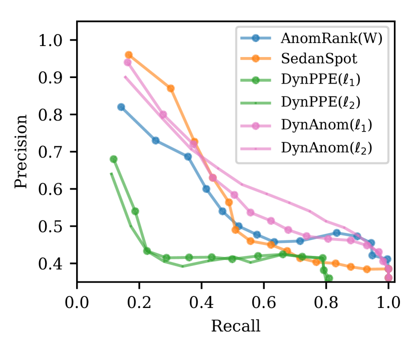
Figure 3. Precision-Recall Curve

Table 6. The precision of top-250 anomalies

Algorithms	Precision
NetWalk	OOM
AnomRankW	0.5400
SedanSpot	0.5640
DynPPE($\ell_{1}$)	0.4160
DynPPE($\ell_{2}$)	0.3920
DynAnom($\ell_{1}$)	0.5840
DynAnom($\ell_{2}$)	0.6120

ENRON graph records the emails involved in the notorious Enron company scandal, and it has been intensively studied in (Eswaran and Faloutsos, 2018; Chang et al., 2021; Yoon et al., 2019). Although ENRON graph has no explicit anomaly annotation, a common practice (Chang et al., 2021; Yoon et al., 2018) is to visualize the detected anomaly score against time and discover the associated real-world events. Likewise, Figure 4 plots the detected peaks side-by-side with other strong baselines . We find that DynAnom shares great overlaps with meaningful peaks and detects more prominent peak at Marker.1 when Enron got investigated for the first time, demonstrating its effectiveness for sensible change discovery . For better interpretation, we annotate the peaks associated to the events collected from the Enron Timeline , and present some milestones as followings:

• :(2000/08/23) Investigated Enron when stock was high.

• :(2001/08/22) CEO was warned of accounting irregularities.

• :(2002/01/30) CEO was replaced after bankruptcy.

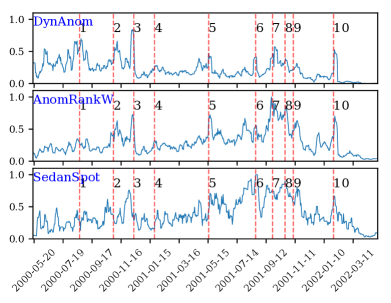
Figure 4. The anomaly scores of ENRON graph. DynAnom well correlates with other baselines, and detect novel peaks at beginning.

6.5. Case Study: Localize Changes in Person’s life over Real World Graph

To demonstrate the scalability and usability of DynAnom, we present an interesting case study over our constructed large-scale PERSON graph, which records the structure and intensity of person-event interaction history. We apply DynAnom to track public figures (Joe Biden, Arnold Schwarzenegger, Al Franken) of the U.S. from 2000 to 2022 on a yearly basis, and visualize their changes by $\ell_{1}$-distance, together with annotated peaks in Figure 5.

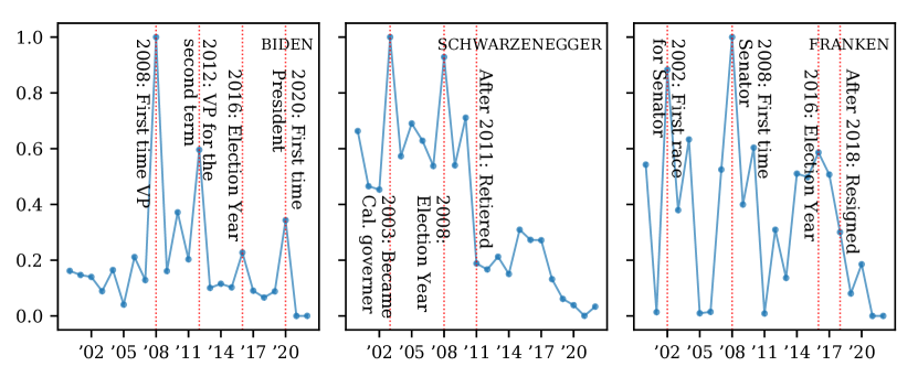
Figure 5. The yearly changes of public figures in PERSON graph from 2000-2022: The detected peaks are well correlated to the major events of the individuals as we annotated.

As we can see, Biden has his greatest peak in year 2008 when he became the 47-th U.S. Vice President for the very first time, which is considered to be his first major advancement. The second peak occurs in 2012 when he won the re-election. This time the peak has smaller magnitude because he was already the VP, thus the re-election caused less difference in him, compared to his transition in 2008. The third peak is in 2020 when he became the president, the magnitude is even smaller as he had been the VP for 8 years without huge context changed. Similarly, the middle sub-figure captures Arnold Schwarzenegger’s transition to be California Governor in 2003, and high activeness in election years. Al Franken is also a famous comedian who shifted career to be a politician in 2008, the peaks well capture the time when he entered political area and the election years. Table 8 lists full events in Appendix C. This resources could bring more opportunities for knowledge discovery and anomaly mining studies in the graph mining community.

Moreover, based on our current Python implementation, it took roughly 37.8 minutes on a 4-core CPU machine to track the subset of three nodes over the PERSON graph, which has more than 600k nodes and 8.7 million edges. Both presented results demonstrate that our proposed method has great efficiency and usability for practical subset node tracking.

7. Discussion and Conclusion

In this paper, we propose an unified framework DynAnom for subset node anomaly tracking over large dynamic graphs. This framework can be easily applied to different graph anomaly detection tasks from local to global with a flexible score function customized for various application. Experiments show that our proposed framework outperforms current state-of-the-art methods by a large margin, and has a significant speed advantage (2.3 times faster) over large graphs. We also present a real-world PERSON graph with an interesting case study about personal life changes, providing a rich resource for both knowledge discovery and algorithm benchmarking. For the future work, it remains interesting to explore different type of score functions, automatically identify the interesting subset of nodes as better strategies for tracking global-level anomaly, and further investigate temporal-aware PageRank as better node representations.

Appendix A Proof of Thm. 1

Proof.

By the invariant property in Lemma 2, we have

(13) $$p_{s}(i)+\alpha r_{s}(i)=(1-\alpha)\sum_{x\in N^{in}(i)}\frac{w_{(x,i)}p_{s}(x)}{d(x)}+\alpha\times 1_{i=s},\forall i\in\mathcal{V},$$

Initially, this invariant holds and keeps $\frac{r_{s}(i)}{d(i)}\leq\epsilon$ after applying Algo.1. When the new edge $(u,v,\Delta w_{(u,v)})$ arrives, it changes the out-degree of $u$, breaking up the balance for all invariant involving $d(u)$. Our goal is to recover such invariant by adjusting small amount of $p_{s},r_{s}$. While such adjustments may compromise the quality of PPVs, we could incrementally invoke Algo.1 to update $p_{s}$ and $r_{s}$ for better accuracy afterwards. We denote the initial vectors as $p_{s},r_{s},d$ and post-change vectors as $p^{\prime}_{s},r^{\prime}_{s},d^{\prime}$.

As $d^{\prime}(u)$ is involved in $p_{s}(u)/d^{\prime}(u)$, one need to have $p^{\prime}_{s}(u)$ such that $p_{s}(u)/d(u)=p^{\prime}_{s}(u)/d^{\prime}(u)$, i.e. the invariant maintenance of Equ. (13). The updated amount of weight is $\delta w_{(}u,v)$, which indicates $p^{\prime}_{s}(u)=(d(u)+\Delta w_{(u,v)})p_{s}(u)/d(u)$. So, we have

(14) $$p^{\prime}_{s}(u)=p_{s}(u)\frac{\sum_{v\in\operatorname{Nei}(u)}w_{(u,v)}+\Delta w_{(u,v)}}{\sum_{v\in\operatorname{Nei}(u)}w_{(u,v)}}.$$

Hence, we reach Equ. 14 implies that we should scale up $p_{s}(u)$ to recover balance. This strategy is the general case of Zhang et al. (2016) for unweighted graphs where $\Delta w_{(u,v)}=1$.

However, once we assign $p^{\prime}_{s}(u)$, it breaks the invariant for $u$ since $p_{s}(u)+\alpha r_{s}(u)\neq p^{\prime}_{s}(u)+\alpha r_{s}(u)$. Likewise, we maintain this equality by introducing $r^{\prime}_{s}(u)$:

$$p_{s}(u)+\alpha r_{s}(u) =p_{s}^{\prime}(u)+\alpha r_{s}^{\prime}(u)$$

Substitute $$p^{\prime}_{s}(u)$$ from eq.5

$$=p_{s}(u)+\frac{\Delta w_{(u,v)}p_{s}(u)}{d(u)}+\alpha r_{s}^{\prime}(u),\allowdisplaybreaks$$

$$\Longrightarrow\alpha r_{s}^{\prime}(u)-\alpha r_{s}(u) =-\frac{\Delta w_{(u,v)}p_{s}(u)}{d(u)},\allowdisplaybreaks$$

(15) $$r_{s}^{\prime}(u) =r_{s}(u)-\frac{\Delta w_{(u,v)}p_{s}(u)}{\alpha d(u)}$$

Equ. (15) implies that we should decrease $r_{s}(u)$. From a heuristic perspective, it’s consistent to the behavior of BCA-algorithm which keeps taking mass from $r_{s}$ to $p_{s}$. In this updating case, we artificially create mass for $p^{\prime}_{s}$ at the expense of $r_{s}$’s decrements. When $\Delta w_{(u,v)}=1$ in case of unweighted graphs, this update rule is also equivalent to Zhang et al. (2016).

So far, we have the updated $p^{\prime}_{s}(u)$ and $r^{\prime}_{s}(u)$ so that all nodes (without direct edge update, except for $v$) keep the invariant hold. However, due to the introduction of $\Delta w_{(u,v)}$, the shares of mass pushed to $v$ is changes, breaking the invariant for $v$ as shown below:

$$p_{s}(v)+\alpha r_{s}(v) \neq(1-\alpha)\Bigl{(}\frac{(w_{(u,v)}+\Delta w_{(u,v)})p^{\prime}_{s}(u)}{d^{\prime}(u)}\Bigr{.}$$

$$\Bigl{.}+\sum_{x\in N^{in}(v)\setminus\{u\}}\frac{w_{(u,x)}p_{s}(x)}{d(x)}\Bigr{)}+\alpha\times 1_{t=s}$$

In order to recover the balance with minimal effort, we should update $r_{s}(v)$ instead of $p_{s}(v)$. The main reason is that any change in $p_{s}(v)$ will break the balance for $v$’s neighbors, similar to the breaks incurred by the change of $p_{s}(u)$. We present the updated $r^{\prime}_{s}(v)=r_{s}(v)+\Delta$ as following:

$$p_{s}(v)+\alpha\Bigl{(}r_{s}(v)+\Delta\Bigr{)}=(1-\alpha)\Bigl{(}\frac{\Delta w_{(u,v)}p^{\prime}_{s}(u)}{d^{\prime}(u)}+\Bigr{.}$$

(16) $$\Bigl{.}\sum_{x\in N^{in}(v)}\frac{w_{(u,x)}p_{s}(x)}{d(x)}\Bigr{)}+\alpha 1_{t=s}.$$

Note that $p^{\prime}_{s}(u)/d^{\prime}(u)=p_{s}(u)/d(u)$, and

$$p_{s}(v)+\alpha r_{s}(v)=(1-\alpha)\sum_{x\in N^{in}(v)}\frac{w_{(x,v)}p_{s}(x)}{d(x)}.$$

Reorganize Equ. (16) and cancel out $p_{s}(v),r_{s}(v)$, we have

$$\Delta =\frac{(1-\alpha)}{\alpha}\frac{\Delta_{w_{(u,v)}}p_{s}(u)}{d(u)}\allowdisplaybreaks$$

(17) $$r_{s}^{\prime}(v) =r_{s}(v)+\frac{(1-\alpha)}{\alpha}\frac{\Delta_{w_{(u,v)}}p_{s}(u)}{d(u)}$$

Combining Equ. (14),(15), and (17), we prove the theorem. ∎

Remark 1.

The above proof mainly follows from (Zhang et al., 2016) where unweighted graph is considered while we consider weighted graph in our problem setting.

Appendix B Proof of Thm. 2

Before we proof the theorem, we present the known time complexity of IncrementPush as in the following lemma.

Lemma 1 (Time complexity of IncrementPush (Guo et al., 2021)).

Suppose the teleport parameter of obtaining PPR is $\alpha$ and the precision parameter is $\epsilon$. Given current weighted graph snapshot $\mathcal{G}_{t}$ and a set of edge events $\Delta E_{t}$ with $|\Delta E_{t}|=m$ , the time complexity of IncrementPush is $\mathcal{O}(m/\alpha^{2}+\bar{d}^{t}/(\epsilon\alpha^{2})+1/(\epsilon\alpha))$ where $\bar{d}^{t}$ is the average node degree of current graph $\mathcal{G}_{t}$.

Proof.

The total time complexity of our instantiation DynAnom has components, which correspond to three steps in Algo. 2. The run time of step 1, IncrementPush is $\mathcal{O}(m/\alpha^{2}+\bar{d}^{t}/(\epsilon\alpha^{2})+1/(\epsilon\alpha))$ by Lemma 1. The run time of step 2, DynNodeRep is bounded by $\mathcal{O}(n)$ as the component of DynNodeRep is the procedure of the dimension reduction by using two hash functions. The calculation of two has functions given $\bm{p}_{s}$ is linear on $|\operatorname{supp}(\bm{p}_{s})|$, which is $|\operatorname{supp}(\bm{p}_{s})|\leq n$. Finally, the instantiation of our score function is also linear on $n$. Therefore, the whole time complexity is dominated by $\mathcal{O}(km/\alpha^{2}+k\bar{d^{t}}/(\epsilon\alpha^{2})+k/(\epsilon\alpha)+kTs)$ where $s$ is the maximal allowed sparsity defined in the theorem. We proof the theorem. ∎

Appendix C Timelines of real world graphs

We list the real-world events for the ENRON and PERSON graph in table 7 and 8.

Table 7. The events in Enron scandal timeline

Index	Date	Event Description
1	2000/08/23	Stock hits all-time high of $90.56. the Federal Energy Regulatory Commission orders an investigation.
2	2000/11/01	FERC investigation exonerates Enron for any wrongdoing in California.
3	2000/12/13	Enron announces that president and chief operating officer Jeffrey Skilling will take over as chief executive in February. Kenneth Lay will remain as chairman.
4	2001/01/25	Analyst Conference in Houston, Texas. Skilling bullish on the company. Analysts are all convinced.
5	2001/05/17	"Secret" meeting at Peninsula Hotel in LA – Schwarzenegger, Lay, Milken.
6	2001/08/22	Ms Watkins meets with Lay and gives him a letter in which she says that Enron might be an "elaborate hoax."
7	2001/09/26	Employee Meeting. Lay tells employees: Enron stock is an "incredible bargain." "Third quarter is looking great."
8	2001/10/22	Enron acknowledges Securities and Exchange Commission inquiry into a possible conflict of interest related to the company’s dealings with the partnerships.
9	2001/11/08	Enron files documents with SEC revising its financial statements to account for $586 million in losses. The company starts negotiations to sell itself to head off bankrutcy.
10	2002/01/30	Stephen Cooper takes over as Enron CEO.

Table 8. The person events of Schwarzenegger and Franken

Year	Major Event
Arnold Schwarzenegger
2003	Arnold Schwarzenegger won the California gubernatorial election as his first politician role
2008	Arnold began campaigning with McCain as the key endorsement for McCain’s presidential campaign
2010	mid-term election
2011	Arnold reached his term limit as Governor and returned to acting
Al Franken
2002	Al Franken consider his first race for office due to the tragedy of Minnesota Sen. Paul Wellstone.
2004	The Al Franken Show aired
2007	Al Franken announced for candidacy for Senate.
2008	Al Franken won election.
2012	Al Franken won re-election.
2018	Al Franken resigned

Appendix D Hyper-parameter Settings

we (re)implement the algorithms in Python to measure comparable running time. We list the hyper-parameter in Table 9.

Table 9. The hyper-parameter configurations of algorithms in experiments.

Algorithm	Hyper-parameter Settings
AnomRank	alpha = 0.5 (default ) ,  epsilon = 1e-2 (default ) or 1e-6 (for better accuracy)
SedanSpot	sample-size = 500 (default settings)
NetWalk	epoch_per_update=10, dim=128, default settings for the rest parameters
DynAnom & DynPPE	For exp1 and exp2: alpha = 0.15, minimum epsilon = 1e-12 , dim=1024; For exp2: we keep track of the top-100 high degree nodes for graph-level anomaly. For case studies: alpha = 0.7, the rest are the same.

Appendix E Experiment Details

Infrastructure

: We conduct our experiment on machine with 4-core Intel i5-6500 3.20GHz CPU, 32 GB memory, and GeForce GTX 1070 GPU (8 GB memory) on Ubuntu 18.04.6 LTS.

Datasets:

For DARPA dataset: we totally track 200 anomalous nodes, and 151 of them have at least one anomalous edge after initial snapshot, the ground-truth of node-level anomaly is derived from the annotated edge as aforementioned. For EU-CORE dataset: Since EU-CORE dataset does not have annotated anomalous edges, we randomly select 20 snapshots to inject artificial anomalous edges using two popular injection methods, which are similar to the approach used in (Yoon et al., 2019). For each selected snapshot in EU-CORE-S, we uniformly select one node,$u_{high}$, from the top 1% high degree nodes, and injected 70 multi-edges connecting the selected node to other 10 random nodes which were not connected to $u_{high}$ before, which simulates the structural changes. In each selected snapshot in EU-CORE-L, we uniformly select 5 pairs of nodes, and injected edge connect each pair with totally 70 multi-edges as anomaly, which simulates the sudden peer-to-peer communication. We include all datasets in our supplementary materials.