Beyond the ABCDs: A better matrix method for geometric optics by using homogeneous coordinates

Abstract

Geometric optics is often described as tracing the paths of non-diffracting rays through an optical system. In the paraxial limit, ray traces can be calculated using ray transfer matrices (colloquially, ABCD matrices), which are $2\times 2$ matrices acting on the height and slope of the rays. A known limitation of ray transfer matrices is that they only work for optical elements that are centered and normal to the optical axis. In this article, we provide an improved $3\times 3$ matrix method for calculating paraxial ray traces of optical systems that is applicable to how these systems are actually arranged on the optical table: lenses and mirrors in any orientation or position (e.g. in laboratory coordinates), with the optical path zig-zagging along the table. Using projective duality, we also show how to directly image points through an optical system using a point transfer matrix calculated from the system’s ray transfer matrix. We demonstrate the usefulness of these methods with several examples and discuss future directions to expand applications of this technique.

I Introduction

Geometric optics describes light as non-diffracting rays traveling through media and surfaces using the laws of reflection and refraction. Assuming the optical system of lenses, mirrors, etc., has a rotational axis of symmetry (the optical axis) we can define the paraxial approximation as the limit where the ray height $h$ relative to the axis is much smaller in magnitude than other lengths in the system, such as radii of curvature or focal lengths, and the slope $m$ the ray makes with the optical axis has a magnitude much smaller than one. In this paraxial limit, the effect of optical elements such as lenses and mirrors may be approximated by linear functions of a ray’s height and slope. This approximation is often the first step in designing optical systems and is also one of the first optics topics presented to students (yielding the Gaussian and Newtonian image equations, the lensmaker’s equation, etc.).

Under these conditions, the laws of reflection and refraction at planar and spherical surfaces may be replaced by their Taylor series approximations to first order in $h$ and $m$, and therefore may be expressed as matrix equations.Halbach (1964); Gerrard and Burch (1994); Pedrotti et al. (2007); Hecht (2017) These matrices are known as ray transfer matrices (RTM), or “ABCD matrices” after their typical parameterization. In this article, we revisit the ABCD matrices from a geometric perspective, rather than a strictly algebraic one, and use geometric insight to expand the functionality of our matrix representation. We do this by introducing a homogeneous coordinate representation of lines, showing that the ray transfer matrices are already applicable in this system, and then adding geometric transformations to our set of allowed operations. The ideas we present here are implicit in advanced treatments of optics, for example, the geometric optics chapters of Born and Wolf,Born and Wolf (1999) but have not been previously fleshed out into an easy-to-use form. We fill in the missing steps, and the end result is a set of relatively simple algebraic rules for modelling almost any common optical setup.

The key new calculational tool we use, expressing lines and points in homogeneous coordinates (defined in Sec. III), is well known in the computer graphics community where it is used to express rotations, translations, affine transformations (e.g. shears), and perspective transformations as matrices.Pharr et al. (2016) Homogeneous coordinates are also a natural setting for projective geometry (particularly oriented projective geometryStolfi (2014)) which was a common mathematical description of geometric optics from the Italian RenaissanceCoxeter (2003) up until the mid-1900s.Cambi (1959) Unfortunately, work in this area was largely abandoned when digital computers became viable for full, non-paraxial ray tracing using the exact laws of reflection and refraction.Feder (1963); Wynne and Wormell (1963)

In our work, we express rays as oriented lines in homogeneous coordinates and identify the matrices that correspond to common optical elements favoring direct ray tracing calculations using the laws of reflection and refraction. This takes us beyond the augmented ABCD matrices used by some authorsGerrard and Burch (1994); Arnaud (1976); Shaomin (1985); Siegman (1986); Tovar and Casperson (1995); Lin and Sung (2006); Lin and Hsueh (2009); Lin (2014) to a fully consistent geometric treatment. A better understanding of the geometry underlying the ray transfer matrices is also helpful in solving the inverse problem of finding a set of optical elements needed to produce a given optical transformation.Liu and Brenner (2008); Tovar and Casperson (1997) Most optical modelling involves the analysis of rays through the optical system, but by invoking one other new math tool, projective duality, we expand this idea to analyzing points as well. In other words, we can calculate images directly without tracing rays. We call this transformation of points the point transfer matrix, which we obtain from an algebraic manipulation of the ray transfer matrix.

The outline of this article follows. We begin in Section II with a review of the paraxial ray transfer matrices as typically used in two-dimensional or axially symmetric optical systems. Next we show how RTMs are a disguised form of general linear operators on the vector space of lines represented in homogeneous coordinates (Section III). Because we are using homogeneous coordinates, we can also consider optical elements decentered or rotated with respect to the optical axis, which we discuss in Section IV along with an example. Careful treatment of algebraic signs allows us to preserve the propagation direction of our rays, which we explore in Section V to derive orientation-preserving RTMs for reflective elements. By requiring a coincident point and line to remain so after imaging, we find a key new result that we call point transfer matrices (PTMs) (Section VI), and provide some examples demonstrating how PTMs simplify imaging calculations and the analysis of optical systems (Section VII). Finally, we close in Section VIII with a discussion of what would be required to extend these results to three-dimensional systems and the complications that arise therein.

The Supplemental MaterialsSMN contain an alternative derivation of the PTMs using Grassmann exterior algebra (an algebra that uses different “grades” to represent the geometric ideas of lines, areas, and volumes), leading to a compact proof of the Scheimpflug principle of tilt-shift photography, as well as example python code for implementing our work. In particular, the python code contains calculations for the examples in this main text and additional examples that we omitted to save space.

II Ray transfer matrices

Before introducing our new concepts, we will briefly review the ray transfer matrices as conventionally used. We refer readers to Refs. Halbach, 1964; Gerrard and Burch, 1994; Pedrotti et al., 2007; Hecht, 2017 for detailed derivations. Several conventions exist in the literature regarding the ordering of elements and the implementation of the index of refraction. We will follow the convention of the textbook by the Pedrottis.Pedrotti et al. (2007)

We define an incoming ray vector ${r}=(h,m)^{T}$ representing a ray with slope $m$ relative to the optical axis and crossing the input plane of the optical system at height $h$. (We use ^T to indicate matrix transposition.) The coordinate origins of the object/image spaces are centered on the first/last surfaces of the optical system, as shown in Fig 1. The incoming ray transforms into the outgoing ray ${r}^{\prime}=(h^{\prime},m^{\prime})^{T}$ through the relation

$$\begin{pmatrix}h^{\prime}\\ m^{\prime}\end{pmatrix}=\begin{pmatrix}A&B\\ C&D\end{pmatrix}\begin{pmatrix}h\\ m\end{pmatrix},$$ (1)

where $A,B,C,D$ are real-valued constants obeying $AD-BC\neq 0$ such that this ray transfer matrix is invertible. In particular, the matrix determinant is equal to the ratio of the incoming and outgoing indices of refraction, $AD-BC=n/n^{\prime}$, which is often unity for common optical systems.Pedrotti et al. (2007) This makes the determinant a useful check on computational results. The relationship described by Eq. (1) is shown schematically in Fig. 1.

Figure 1: Ray transfer matrix. The incoming ray ${r}$ enters the optical system (gray box) and is transformed into the outgoing ray ${r}^{\prime}$ according to the ABCD matrix in Eq. (1). The slopes of the rays are exaggerated for clarity. Note that the incoming coordinate system $(x,y)$ has its origin at the input plane of the system and that the outgoing coordinate system $(x^{\prime},y^{\prime})$ has its origin at the output of the system. The horizontal line represents the optical axis of the system.

Note that some references, such as the popular textbook by Hecht,Hecht (2017) use different conventions for the ray vectors and matrices. A common choice is to multiply the slope in the ray vector by the index of refraction, yielding the “reduced slope.” We prefer to use the geometric slope to avoid complications in our transformation operators (Sec. V).

The ray transfer matrices are particularly useful because whole optical systems may be summarized by the product of the matrices of their components, with the sequence written from right to left (first element right-most). If we exchange the input and output ends of the optical system (or equivalently, reverse time), the resulting ray transfer matrix is the matrix inverse of the original system RTM.

III Rays and ray transfer matrices in homogeneous coordinates

In this section we introduce a homogeneous representation of lines in a plane, which consists of a set of three coefficients, as opposed to the more familiar height and slope definition above. This will require us to replace the $2\times 2$ ABCD matrices with $3\times 3$ ray transfer matrices. The additional row and column provide the additional degrees of freedom that we need to implement the key results that follow in later sections.

Given a ray vector ${r}=(h,m)^{T}$, we could equivalently say that the ray falls along the line given by the equation $y=mx+h$. It will be helpful to us to rewrite the equation for the line in the form $ax+by+c=0$ and use the coefficients $a$, $b$, and $c$ to define a vector representation of the line: ${r}=(c,a,b)^{T}$. (Note the order of the coefficients, which we’ve chosen to facilitate comparisons of our matrices with the conventional version). For example, our standard ray above is described by the rearranged equation $-mx+y-h=0$, corresponding to the ray vector ${r}=(-h,-m,1)^{T}$. Multiplying the line equation or the vector ${r}$ by a positive scalar does not change the geometric line it represents, so this is a homogeneous representation of the line (Fig. 2). Although it is not necessary for our calculations, if we wish to normalize the ray vector ${r}$, a convenient choice is to require $a^{2}+b^{2}=1$. With this normalization it turns out that $a$ and $b$ equal the direction cosines of the line with respect to the $x$ and $y$ axes, respectively, and $|c|$ is the perpendicular distance from the line to the coordinate origin. If care is taken with signs during calculations (see Sec. V for how reflections must be handled), the rays expressed this way are oriented (have a well-defined forward direction). For a ray $(c,a,b)^{T}$, the direction of propagation, measured counter-clockwise from the positive $x$-axis to the forward-going side of the ray, is the angle $\phi=\arctan(-a/b),$ where it is necessary to add $\pi$ radians to the value of $\phi$ in the case $b<0$ to match the forward direction of the ray.not The propagation direction of paraxial rays in our convention is given by the sign of $b$: left-to-right rays have $b>0$ and right-to-left rays have $b<0$ (see Sec. V for more detail).

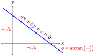
Figure 2: (Color online) Representation of the ray $(c,a,b)^{T}$ as the oriented line $ax+by+c=0$. The coefficients of the equation can be used to calculate the $x$- and $y$-intercepts, slope, and distance from the origin. Note that for this particular oriented line, $a,b>0$ and $c<0$.

If the conventional $2\times 2$ ray transfer matrix of an optical system is known, the corresponding ray transfer matrix in homogeneous coordinates for nonreflecting systems (see Sec. V for the reflecting case) is

$$M={\small\begin{pmatrix}A&B&0\\ C&D&0\\ 0&0&1\end{pmatrix}}.$$

Using the height-slope definition of the ray vectors, the ray transfer equation reads

$${\small\begin{pmatrix}-h^{\prime}\\ -m^{\prime}\\ 1\end{pmatrix}}={\small\begin{pmatrix}A&B&0\\ C&D&0\\ 0&0&1\end{pmatrix}\begin{pmatrix}-h\\ -m\\ 1\end{pmatrix}}.$$

Compare this with Eq. 1. The RTMs for common optical elements are summarized in Table 1. The additional row and column will have no apparent purpose at first, but they provide additional degrees of freedom that we will exploit later for coordinate transformations to represent decentered and rotated optical elements (Sec. IV), consistent handling of orientation (Sec. V), and imaging of points (Sec. VI).

Table 1: Summary of ray transfer and point transfer matrices

Element	RTM	PTM
General form for centered elements	$\begin{pmatrix}A&B&0\\ C&D&0\\ 0&0&1\end{pmatrix}$	$\begin{bmatrix}D&-C&0\\ -B&A&0\\ 0&0&AD-BC\end{bmatrix}$
Thin lens of focal length $f$	$\begin{pmatrix}1&0&0\\ -1/f&1&0\\ 0&0&1\end{pmatrix}$	$\begin{bmatrix}1&1/f&0\\ 0&1&0\\ 0&0&1\end{bmatrix}$
Free-space propagation over distance $d$	$\begin{pmatrix}1&d&0\\ 0&1&0\\ 0&0&1\end{pmatrix}$	$\begin{bmatrix}1&0&0\\ -d&1&0\\ 0&0&1\end{bmatrix}$
Refraction at a flat normal surface from index of refraction $n$ to $n^{\prime}$	$\begin{pmatrix}1&0&0\\ 0&n/n^{\prime}&0\\ 0&0&1\end{pmatrix}$	$\begin{bmatrix}n/n^{\prime}&0&0\\ 0&1&0\\ 0&0&n/n^{\prime}\end{bmatrix}$
Refraction at a curved surface centered on the axis from index of refraction $n$ to $n^{\prime}$ with radius of curvature $R$ ($R>0$ is convex)	$\begin{pmatrix}1&0&0\\ \frac{n-n^{\prime}}{Rn^{\prime}}&\frac{n}{n^{\prime}}&0\\ 0&0&1\end{pmatrix}$	$\begin{bmatrix}\frac{n}{n^{\prime}}&-\frac{n-n^{\prime}}{Rn^{\prime}}&0\\ 0&1&0\\ 0&0&\frac{n}{n^{\prime}}\end{bmatrix}$
Reflection at a plane surface	$\begin{pmatrix}-1&0&0\\ 0&1&0\\ 0&0&-1\end{pmatrix}$	$\begin{bmatrix}-1&0&0\\ 0&1&0\\ 0&0&-1\end{bmatrix}$
Reflection at a spherical surface with radius of curvature $R$ ($R>0$ is convex)	$\begin{pmatrix}-1&0&0\\ 2/R&1&0\\ 0&0&-1\end{pmatrix}$	$\begin{bmatrix}-1&2/R&0\\ 0&1&0\\ 0&0&-1\end{bmatrix}$
Translation by displacement $(u,v)$	$\begin{pmatrix}1&-u&-v\\ 0&1&0\\ 0&0&1\end{pmatrix}$	$\begin{bmatrix}1&0&0\\ u&1&0\\ v&0&1\end{bmatrix}$
Rotation by angle $\theta$	$\begin{pmatrix}1&0&0\\ 0&\cos\theta&-\sin\theta\\ 0&\sin\theta&\cos\theta\end{pmatrix}$	$\begin{bmatrix}1&0&0\\ 0&\cos\theta&-\sin\theta\\ 0&\sin\theta&\cos\theta\end{bmatrix}$

IV Coordinate transformations

The $2\times 2$ ray transfer matrices assume that the optical system has axial symmetry. In our expanded $3\times 3$ formulation we can incorporate off-axis and rotated elements.Gerrard and Burch (1994); Siegman (1986); Tovar and Casperson (1995) We add to our repertoire of ray transfer matrices a matrix $R_{\theta}$ that rotates a ray by angle $\theta$ counter-clockwise about the origin and a matrix $T_{u,v}$ that translates a ray by $u$ in the $x$-direction and $v$ in the $y$-direction.

$$R_{\theta} ={\small\begin{pmatrix}1&0&0\\ 0&\cos\theta&-\sin\theta\\ 0&\sin\theta&\cos\theta\end{pmatrix}}, T_{u,v} ={\small\begin{pmatrix}1&-u&-v\\ 0&1&0\\ 0&0&1\end{pmatrix}}.$$ (2)

Note that a translation matrix with only horizontal displacement is equivalent to the propagation matrix from Table 1. These coordinate transformation matrices are exact in the sense that they are not linear approximations with respect to their arguments, in contrast to the refractive sufrace matrices and spherical mirror matrix in Table 1.

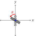
Figure 3: (Color online) The effects of applying the rotation operator $R_{\theta}$ (left) and translation operator $T_{u,v}$ (right) to an optical element using Eq. (4).

The ray transfer matrices given earlier in Table 1 assume the elements are located at the origin and normal to the optical axis. We can use the $T$ and $R$ matrices above to walk between optical elements without the restriction that they lie on the optical axis or that they are oriented normal to the original optical axis. We can represent an element $M$ that is rotated and then translated into a new position by

$$M^{\prime}=MR_{\theta}^{-1}T_{u,v}^{-1},$$ (3)

where the outgoing coordinate axes are centered and aligned with the axis of the optical element, rather than the original optical axis. Note that the inverses are simply $R_{\theta}^{-1}=R_{-\theta}$ and $T_{u,v}^{-1}=T_{-u,-v}$. Eq. (3) respects the traditional application of the ray transfer matrices, where the input rays and output rays are specified in different coordinate systems. The input rays are measured relative to a coordinate origin located at the first surface of the optical system, and the output rays are measured relative to a coordinate origin located at the final surface, as shown earlier in Fig. 1. As a simple example of Eq. (3), take $M$ to be the identity matrix and then translate along the axis by a distance $d$. The resulting matrix is

$$M^{\prime}=IT_{d,0}^{-1}={\small\begin{pmatrix}1&d&0\\ 0&1&0\\ 0&0&1\end{pmatrix}},$$

which is exactly the expanded form of the propagation matrix in Table 1.

In some applications (e.g. when mechanical dimensions are needed for prototyping an optomechanical layout) it is preferable to restore the original coordinate system. This choice of output coordinates is accomplished by

$$M^{\prime}=T_{u,v}R_{\theta}MR_{\theta}^{-1}T_{u,v}^{-1}.$$ (4)

This construction places the image space coordinate system to be coincident with the object space coordinate system, which contrasts with the typical convention for ray transfer matrices that treats the object space and image space independently.

Several expressions other than Eq. (2) are found in the literature for handling decentered or tilted optical elements.Gerrard and Burch (1994); Arnaud (1976); Shaomin (1985); Siegman (1986); Tovar and Casperson (1995); Lin and Sung (2006); Lin and Hsueh (2009); Lin (2014) For example, the rotation operator is often given as Gerrard and Burch (1994); Siegman (1986)

$$R^{\prime}_{\theta}={\small\begin{pmatrix}1&0&0\\ 0&1&-\theta\\ 0&0&1\end{pmatrix}}.$$

This operator is in fact not a rotation but a shear, a vertical displacement proportional to the horizontal coordinate. A shear is approximately equal to a rotation for sufficiently small angles, but we prefer the exact rotation formalism.

The benefit we gain over other implementations is that our Eq. (2) does not require small parameters, for example, $|\theta|\ll 1$ in the rotation matrix, because we are transforming the whole coordinate system rather than just the rays themselves. In particular, plane mirrors of any orientation may be exactly modelled (see Sec. V), allowing the model to include, for example, path-folding mirrors along a beam. So long as our rays do not stray too far from our transformed optical axis, the paraxial approximation is still valid even if the mechanical layout of the system is not along a single axis. A similar method is described by LinLin (2014) for transforming coordinates in non-paraxial ray tracing (e.g. for implementation by computers), but Lin does not make the connection that these results apply to the paraxial case as well.

IV.1 Example: tilted window

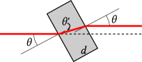
Figure 4: (Color online) Tilted window of thickness $d$ and index of refraction $n$ at an angle $\theta$ relative to normal incidence. The angle of incidence inside the window is denoted $\theta^{\prime}$. The path of the ray is shown as a thick red line, with the original optical axis as a dashed line.

Consider a window of thickness $d$ and index of refraction $n$ tilted by a small angle $\theta$ (Fig. 4). The ray transfer matrix for this system referenced back to the incoming coordinate system is (remembering to read the order of terms from right to left)

$$M =\underbrace{R_{\theta}T_{d,0}}_{\shortstack{\scriptsize return to\\ \scriptsize original coords.}}\underbrace{M_{\text{ref}}(n,1)}_{\shortstack{\scriptsize back \\ \scriptsize surface}}\underbrace{T_{d,0}^{-1}}_{\shortstack{\scriptsize window \\ \scriptsize thickness}}\underbrace{M_{\text{ref}}(1,n)}_{\shortstack{\scriptsize front \\ \scriptsize surface}}\underbrace{R_{\theta}^{-1}}_{\text{rotate}},$$

$$\approx{\small\begin{pmatrix}1&-d\left(1-\tfrac{1}{n}\right)&-d\theta\left(1-\tfrac{1}{n}\right)\\ 0&1&0\\ 0&0&1\end{pmatrix}},$$

where $\theta^{2}$ and higher-orders terms have been discarded in keeping with the paraxial approximation (rays must stay near the transformed optical axis). Applying this RTM to an input ray $(0,0,1)^{T}$ coincident with the input optical axis gives an output ray

$${\small\begin{pmatrix}1&-d\left(1-\tfrac{1}{n}\right)&-d\theta\left(1-\tfrac{1}{n}\right)\\ 0&1&0\\ 0&0&1\end{pmatrix}\begin{pmatrix}0\\ 0\\ 1\end{pmatrix}}={\small\begin{pmatrix}-d\theta\left(1-\tfrac{1}{n}\right)\\ 0\\ 1\end{pmatrix}},$$

showing that the outgoing ray is parallel to the original optical axis and has been displaced upward by a distance $d\theta\left(1-\tfrac{1}{n}\right)$. This agrees to within the paraxial limit with the direct calculation of the displacement of a ray parallel to the optical axis through a tilted plate using Snell’s Law (e.g. Problem 2-8 of PedrottiPedrotti et al. (2007)), which is

$$\Delta h=\frac{d\sin(\theta-\theta^{\prime})}{\cos(\theta^{\prime})}\approx{d\theta}\left(1-\frac{1}{n}\right),$$

where the angle of incidence of the ray inside the window, $\theta^{\prime}$, is given by $\sin(\theta^{\prime})=\sin(\theta)/n$, and we use the small-angle approximation in keeping with the paraxial limit needed for consistency with the refracting surfaces.

V Orientation and Reflections

Reflections require special attention if we wish to include orientation in our homogeneous representation.Dorst (2020); Stolfi (2014) The convention of direction introduced in Section III can be summarized: for the homogeneous ray ${r}=(c,a,b)^{T}$ representing the line $ax+by+c=0$, the ray is oriented left-to-right if $b>0$ and right-to-left if $b<0$. (This explains our choice of signs for the ray vectors in homogeneous coordinates.) The case $b=0$ (vertical rays) does not occur in the paraxial limit, but we may still identify rays with $a>0$ as going down and rays with $a<0$ as going up. The final case is $a=b=0$, representing the line infinitely far away encircling the plane. For these ideal lines $c>0$ circulates counter-clockwise, and $c<0$ goes clockwise. The null ray vector $(0,0,0)^{T}$ is undefined geometrically.

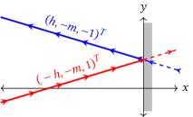
Figure 5: (Color online) Incoming ray (red) striking a plane mirror and reflecting (blue). Both the ray’s slope and its orientation change sign, resulting in the ray vector shown.

Now consider the action of a plane mirror coincident with the $y$ axis on an incoming ray $(c,a,b)^{T}=(-h,-m,1)^{T}$ (Fig. 5). We require both the slope of the ray and its orientation to change signs. The RTM equation that satisfies this is

$${\small\begin{pmatrix}-1&0&0\\ 0&1&0\\ 0&0&-1\end{pmatrix}\begin{pmatrix}-h\\ -m\\ 1\end{pmatrix}}={\small\begin{pmatrix}h\\ -m\\ -1\end{pmatrix}}.$$

The presence of the negative coefficient in the bottom right element of the RTM is the indicator of reflection. Generalizing, we see that the recipe for converting the standard $2\times 2$ RTM of reflective elements into an RTM for oriented homogeneous coordinates is

$$M_{\text{reflective}}=(-1){\small\begin{pmatrix}A&B&0\\ C&D&0\\ 0&0&1\end{pmatrix}}.$$

Specifically, the RTMs for a plane mirror normal to the axis and a spherical mirror with center of curvature on the axis are

$$M_{\text{plane mirror}} ={\small\begin{pmatrix}-1&0&0\\ 0&1&0\\ 0&0&-1\end{pmatrix}},$$

$$M_{\text{sph.~{}mirror}} ={\small\begin{pmatrix}-1&0&0\\ 2/R&1&0\\ 0&0&-1\end{pmatrix}},$$

where $R>0$ for a convex mirror.

V.1 Example: Retroreflector

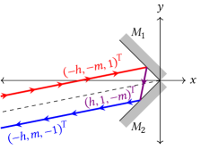
Figure 6: (Color online) Incoming ray (red) striking two mutually perpendicular mirrors ($M_{1}$ and $M_{2}$) and reflecting twice (purple and blue rays). The outgoing ray is antiparallel to the incoming ray. The dashed line shows the bisector of the incoming and outgoing rays, which passes through the intersection of the mirrors.

A retroreflector can be made from a pair of plane mirrors intersecting at right angles (Fig. 6). Using our rotation operator from Eq. (2) we can build a system ray transfer matrix that also respects the orientation of the rays. Note that our rotation angles are $\pm 45^{\circ}$, which are not small. Care must be taken when ordering the RTMs. We’ll assume that the incoming ray ${r}_{0}=(-h,-m,1)^{T}$ first strikes the upper mirror and then strikes the lower mirror. Choosing a different input ray may require the user to change the order of the mirrors, depending on which surface is struck by the ray first.

The RTM for the upper mirror ($M_{1}$) is generated by a $45^{\circ}$ rotation of a plane mirror situated at the origin:

$$M_{1} =R_{45^{\circ}}M_{\text{plane mirror}}R_{45^{\circ}}^{-1},$$ (5)

$$={\small\begin{pmatrix}1&0&0\\ 0&\frac{1}{\sqrt{2}}&-\frac{1}{\sqrt{2}}\\ 0&\frac{1}{\sqrt{2}}&\frac{1}{\sqrt{2}}\end{pmatrix}\begin{pmatrix}-1&0&0\\ 0&1&0\\ 0&0&-1\end{pmatrix}\begin{pmatrix}1&0&0\\ 0&\frac{1}{\sqrt{2}}&\frac{1}{\sqrt{2}}\\ 0&-\frac{1}{\sqrt{2}}&\frac{1}{\sqrt{2}}\end{pmatrix}},$$

$$={\small\begin{pmatrix}-1&0&0\\ 0&0&1\\ 0&1&0\end{pmatrix}}.$$

Similarly, the lower mirror ($M_{2}$) has the RTM

$$M_{2}=R_{-45^{\circ}}M_{\text{plane mirror}}R_{-45^{\circ}}^{-1}={\small\begin{pmatrix}-1&0&0\\ 0&0&-1\\ 0&-1&0\end{pmatrix}}.$$ (6)

We do not need any translation operator between the two mirrors because both mirrors pass through the coodinate origin. The passage of the ray from one mirror to the next is not explictly part of the RTM (other than the order of the optical elements). In other words, the position of the optical elements determines the RTM, not the path of the rays. We choose an incoming ray ${r}_{0}=(-h,-m,1)^{T}$ with $h>0$ such that it will strike mirror $M_{1}$ first, yielding the reflected ray

$${r}_{1}=M_{1}{r}_{0}=(h,1,-m)^{T}.$$

This ray follows the line $h+x-my=0$, propagating from right to left ($b<0$). After the second reflection in $M_{2}$ the final ray is

$${r}_{2}=M_{2}{r}_{1}=(-h,m,-1)^{T},$$

which is antiparallel to the incoming ray, as expected, with a $y$ intercept of $-h$ and propagating right to left ($b<0$). Note also that the method works for any angular separation between the mirrors by including the appropriate angles in Eqs. (5) and (6).

VI Point transfer matrices

Our next goal is to find a linear operator for our optical system that maps points in the object space of our optical system onto points in the image space. We’ll call this operator the point transfer matrix (PTM) of the system in analogy to the ray transfer matrices discussed above. Before we do that, we need to describe how we treat points.

VI.1 Homogeneous points

We express a point with coordinates $[x,y]$ using homogeneous coordinates as a column vector $[1,x,y]^{T}$. (We use square brackets to denote point vectors and round brackets to denote ray vectors to avoid ambiguity.) The added dimension will allow us to rotate and translate points similarly to how we manipulated rays above in Section V. The term “homogeneous” means that we can multiply our point vector by any non-zero scalar without changing its physical meaning. More generally, we express points as ${p}=[w,x,y]^{T}$. We’ll say the points are “normalized” if $w=1$. For other $w\neq 0$, the corresponding physical point is located at position $[x/w,y/w]$. For $w=0$, we interpret the point to be infinitely far away in the direction of slope $y/x$ (taking the limit $w\rightarrow 0^{+}$). The inclusion of infinite (or “ideal”) points is a key feature of homogeneous coordinates. In optics we can use this notation to describe objects infinitely (or practically infinitely) far away, such as distant stars. For additional details about the algebraic relationships between rays and points, please see Section 1 of the Supplemental Materials. Generalizations to three dimensions (and more) can be found in Refs. Stolfi, 2014; Pharr et al., 2016; Doran and Lasenby, 2007; Winitzki, 2020; Dorst et al., 2007; Dorst, 2020.

VI.2 Maintaining coincidence

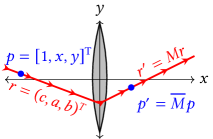
Figure 7: (Color online) Schematic representation of the effects of the ray transfer matrix $M$ and the point transfer matrix $\overline{M}$. The incoming ray $r$ (red line) intesects an object point $p$ (blue point). The lens creates the outgoing ray $r^{\prime}$ which must intersect the image point $p^{\prime}$. The ray vectors are related by the ray transfer matrix by $r^{\prime}=Mr$, and the point vectors are related by the corresponding point transfer matrix by $p^{\prime}=\overline{M}p$.

To motivate our definition for point transfer matrices, consider a ray ${r}=(c,a,b)^{T}$ that passes through a point $[x,y]$, represented by in homogeneous coordinates as the column vector ${p}=[1,x,y]^{T}$ (see Figure 7) The coincidence relationship from above can be stated

$$c+ax+by={p}^{T}{r}=0.$$

Now, let’s image this ray and point through an optical system with ray transfer matrix $M$ and yet-to-be-determined point transfer matrix $\overline{M}$:

$${r}^{\prime}=M{r},\qquad{p}^{\prime}=\overline{M}{p}.$$

The resulting image-space ray ${r}^{\prime}$ and point ${p}^{\prime}$ should also be coincident. This requires

$$0={{p}^{\prime}}^{T}{r}^{\prime}=\left(\overline{M}{p}\right)^{T}\left(M{r}\right)={p}^{T}(\overline{M}^{T}M){r}.$$

The final expression reproduces the original coincidence relation provided that $\overline{M}^{T}M$ is a scalar times the identity matrix, or equivalently, that $\overline{M}^{T}$ is a scalar times $M^{-1}$. A more rigorous derivation (see Section 2 of the Supplemental MaterialsSMN ) shows that the proper scalar factor is $\det(M)$, yielding a point transfer matrix

$$\overline{M}=\det(M)\,(M^{-1})^{T}.$$ (7)

$\overline{M}$ can be calculated using this expression because the ray transfer matrix $M$ is necessarily invertible. If the $2\times 2$ RTM is known, the corresponding PTM is

$$\overline{M}={\small\begin{bmatrix}D&-C&0\\ -B&A&0\\ 0&0&(AD-BC)\end{bmatrix}}.$$ (8)

In the more general case (e.g. when using the coordinate transformations of Sec. V), Eq. (7) holds.

One can also show that $\overline{M}$ is equal to be the adjugateStrang (2006) of the ray transfer matrix $M$, which can be calculated even in the (unphysical) case $\det(M)=0$ using cofactor expansion. When combining optical elements

$$\overline{(M_{2}M_{1})} =\det(M_{2}M_{1})\bigl{(}(M_{2}M_{1})^{-1}\bigr{)}^{T},$$

$$=\det(M_{2})\det(M_{1})(M_{1}^{-1}M_{2}^{-1})^{T},$$

$$=\det(M_{2})(M_{2}^{-1})^{T}\,\det(M_{1})(M_{1}^{-1})^{T}=\overline{M}_{2}\overline{M}_{1},$$

so the PTMs get multiplied in order from right to left, just like the RTMs.

In summary, if we know the ray transfer matrix $M$ of the optical system, which transforms rays using $r^{\prime}=Mr$, then we can use Eq. (7) to calculate the equivalent point transfer matrix $\overline{M}$ that transforms points using $p^{\prime}=\overline{M}p$.

VI.3 Dimensional analysis and units

As in the traditional ABCD formalism, our matrices and vectors contain mixed dimensionality. For completeness, the units of the matrix elements of our RTM and PTM are given here, where $L$ is the unit of length.

$$RTM \sim{\small\begin{pmatrix}1&L&L\\ L^{-1}&1&1\\ L^{-1}&1&1\end{pmatrix}}, PTM \sim{\small\begin{bmatrix}1&L^{-1}&L^{-1}\\ L&1&1\\ L&1&1\end{bmatrix}}.$$

The ray vectors $r$ and point vectors $p$ in normalized form have the dimensions:

$$r \sim(L,1,1)^{T}, p \sim[1,L,L]^{T}.$$

Because we are using homogeneous representations, the vectors may be multiplied by a non-zero dimensionful scalar without changing their geometric meaning.

VII Point-transfer examples

Here we present four examples showing how the PTMs simplify calculations.

VII.1 Deriving Gauss’s lens equation

As a simple example employing the point-transfer matrix consider a thin lens of focal length $f$. Reading the ray transfer matrix elements $ABCD$ from Table 1 and inserting them into the point transfer matrix, we get the equation

$${\small\begin{bmatrix}w^{\prime}\\ x^{\prime}\\ y^{\prime}\end{bmatrix}}={\small\begin{bmatrix}1&1/f&0\\ 0&1&0\\ 0&0&1\end{bmatrix}\begin{bmatrix}1\\ x\\ y\end{bmatrix}}={\small\begin{bmatrix}1+\frac{x}{f}\\ x\\ y\end{bmatrix}},$$ (9)

where the input point is the normalized point at position $[x,y]$. (Recall our sign convention for the coordinates as shown in Fig. 1: $x$ and $x^{\prime}$ increase along the direction of propagation, so that if we follow the usual convention in our optical drawings of light entering from the left, a real object has $x<0$ and a real image has $x^{\prime}>0$.) The resulting output is the normalized point

$$\hat{x}^{\prime} =\frac{x^{\prime}}{w^{\prime}}=\frac{x}{1+(x/f)}=\frac{1}{(1/x)+(1/f)},$$

$$\hat{y}^{\prime} =\frac{y^{\prime}}{w^{\prime}}=\frac{y}{1+(x/f)}=\frac{\hat{x}^{\prime}}{x}\,y.$$

The first line agrees with the Gaussian lens equation giving the location of the image, and the second line gives the image magnification $\hat{x}^{\prime}/x$. The sign of $w^{\prime}$ before normalization gives the orientation of the image: $w^{\prime}>0$ indicates upright and $w^{\prime}<0$ indicates inverted. Our formulation also easily handles the special case when the object (image) point is infinitely far away (the homogeneous weight $w$ ($w^{\prime}$) goes to zero) as well as virtual objects and virtual images, corresponding respectively to $x/w>0$ and $x^{\prime}/w^{\prime}<0$ in the usual case where the optical system is aligned with the $x$-axis.

VII.2 Imaging an infinite object point

To see how the PTMs are used in numerical calculations, consider a simple single-lens camera pointed at the horizon to photograph a star infinitely far away. The parallel rays from the star will converge at the back focal plane of the lens, at a height equal to minus the angular height of the star, times the focal length of the lens.

For concreteness, we can also show this using our point transfer matrix for a star $10$ milliradians above the horizon (Fig. 8) and an $f={50}\,\mathrm{mm}$ lens. The resulting image of the star may be found using the point transfer matrix for a thin lens:

$${\small\begin{bmatrix}1&1/50&0\\ 0&1&0\\ 0&0&1\end{bmatrix}\begin{bmatrix}0\\ -1\\ 0.01\end{bmatrix}}={\small\begin{bmatrix}-0.02\\ -1\\ 0.01\end{bmatrix}}\equiv{\small\begin{bmatrix}1\\ 50\\ -0.5\end{bmatrix}},$$

with implied length units of millimeters. The last step is normalization of the point vector. In this example, the object point is infinitely far away in the direction of slope $=\arctan(0.01/-1)\approx-0.01$ (so the star is above the optical axis ($y>0$) and before the lens ($x<0$)). The final normalized image point has height $y^{\prime}={-0.5}\,\mathrm{mm}$ and is located at $x^{\prime}={50}\,\mathrm{mm}$ after the lens, corresponding with the back focal plane of the lens as expected. Note that we do not need any explicit reference to the light rays to perform the calculation. This example demonstrates one advantage of this method: using homogeneous coordinates allows us to treat both finite and infinite objects/images in the same way without resorting to special cases. A naïve application of Gauss’s lens equation with an infinite object distance would not tell us the vertical position of the image because the linear magnification is undefined in this instance.

Figure 8: (Color online) Calculating the image of a star by treating the star as an object point infinitely far away. The location of the star in homogeneous coordinates is $[0,-1,0.01]^{T}$, the lens has a focal length of $f={50}\,\mathrm{mm}$, and the star’s image is at $[1,x,y]^{T}=[1,50,-0.5]^{T}$ (after normalization). The length units of the vectors are millimeters.

VII.3 Analysis of a compound lens

For our next example (adapted from Examples 6.6 and 6.7 of HechtHecht (2017) – note that we use a different convention for the ray transfer matrices than Hecht), consider a compound lens system with the ray transfer matrix (length units of cm)

$$M=\begin{pmatrix}A&B\\ C&D\end{pmatrix}=\begin{pmatrix}0.867&1.338\\ -0.198&0.848\end{pmatrix},$$

and an object 20 cm in front of the lens with a height of 0.1 cm. We would like to locate the resulting image position and height.

Hecht’s solution has several steps: (1) Extend the system matrix $M$ with a propagation matrix of length 20 cm in front of the lens (for the object position) and a propagation of unknown length $d$ after the lens (for the image position) so that the system matrix now includes both the object and image points. (2) Algebraically set the $B$ element of the resulting product matrix to zero. This enforces the condition that the final ray height is independent of the incoming ray slope (i.e. an image forms). With this constraint, one can solve for the unknown length $d$ to locate the image plane. (3) Identify the magnification as the $A$ element of the resulting matrix. This is true because we set $B=0$ above, meaning that the image ray height only depends on the object ray height, which gives us the magnification.

Our solution is much more direct. First, we construct the point transfer matrix from the original ray transfer matrix (without additional propagations) using Eq. 8 and multiply this into the homogeneous position vector $p=[1,x,y]^{T}$ for the object point. This gives us the image point $p^{\prime}$.

$$p^{\prime}=\overline{M}p ={\small\begin{bmatrix}0.848&0.198&0\\ -1.338&0.867&0\\ 0&0&1\end{bmatrix}\begin{bmatrix}1\\ -20.0\\ 0.1\end{bmatrix}},$$

$$={\small\begin{bmatrix}-3.112\\ -18.678\\ 0.1\end{bmatrix}}\equiv{\small\begin{bmatrix}1\\ 6.002\\ -0.032\end{bmatrix}}.$$

After performing the matrix multiplication, we only need to normalize the resulting image point vector (final step above) to read off the coordinates of the image: ${6.002}\,\mathrm{cm}$ past the lens at a height of ${-0.032}\,\mathrm{cm}$. We’ve been able to replace algebraic multiplication of matrices containing unknown variables and solving for an unknown distance with a direct numerical calculation.

Taking this example one step farther, we can also calculate the front and back focal points of the lens system easily. The back focal point (BFP) is the image of an ideal (infinite) object point on the axis: $[0,-1,0]^{T}$. The image of this point is

$${\small\begin{bmatrix}0.848&0.198&0\\ -1.338&0.867&0\\ 0&0&1\end{bmatrix}\begin{bmatrix}0\\ -1\\ 0\end{bmatrix}}={\small\begin{bmatrix}-0.198\\ -0.867\\ 0\end{bmatrix}}\equiv{\small\begin{bmatrix}1\\ 4.38\\ 0\end{bmatrix}},$$

where the last step is normalization. Reading off the coordinates, the BFP is located 4.38 cm past the final optical surface. To find the front focal point (FFP), we invert the point-transfer matrix of the system (i.e. time reversal) and then follow the same procedure using a ray coming from the reverse direction, $[0,1,0]^{T}$.

VII.4 Misaligned thin lens

A common laboratory task is to take a collimated laser beam and focus it through a pinhole located at the back focal point of a converging lens (for example, to build a spatial filter or to inject the beam into a fiber). If the pinhole is in a fixed position, but the beam doesn’t quite hit the hole, a common remedy is to move the lens slightly in the transverse direction. Another common tactic in the lab is to intentionally tilt a lens to prevent back-reflections from causing interference fringes. As long as these shifts are small, the induced aberrations can be neglected. Here we analyze this configuration for small displacements and small tilts of the lens.

Let’s model our laser beam as a point source infinitely far away, parallel to the optical axis, and ignore diffraction effects. The corresponding (infinite) point vector is ${p}=[0,1,0]^{T}$. In essence, we’re approximating the laser beam as a pencil of parallel rays. We’ll assume a converging lens of focal length $f$. First, let’s consider what happens to the image if we translate the lens by a distance $d$ perpendicular to the optical axis. We do this by applying the point translation operator $\overline{T}_{0,d}$ to the lens PTM. The resulting system matrix $\overline{M}$ is

$$\overline{M} =\overline{T}_{0,d}\,\overline{M}_{\text{thin lens}}(f)\,\overline{T}^{-1}_{0,d},$$

$$={\small\begin{bmatrix}1&0&0\\ 0&1&0\\ d&0&1\end{bmatrix}\begin{bmatrix}1&1/f&0\\ 0&1&0\\ 0&0&1\end{bmatrix}\begin{bmatrix}1&0&0\\ 0&1&0\\ -d&0&1\end{bmatrix}},$$

$$={\small\begin{bmatrix}1&1/f&0\\ 0&1&0\\ 0&d/f&1\end{bmatrix}},$$

and the image point ${p}^{\prime}$ is

$${p}^{\prime}=\overline{M}{p}={\small\begin{bmatrix}1&1/f&0\\ 0&1&0\\ 0&d/f&1\end{bmatrix}\begin{bmatrix}0\\ 1\\ 0\end{bmatrix}}={\small\begin{bmatrix}1/f\\ 1\\ d/f\end{bmatrix}}\equiv{\small\begin{bmatrix}1\\ f\\ d\end{bmatrix}},$$

where the last step is normalization of the point vector. We see that the beam is still focused on the back focal plane ($x^{\prime}=f$), but the focus point is displaced vertically by the same amount as the lens, $d$.

If we tilt the lens, the system PTM is

$$\overline{M} =\overline{R}_{\theta}\,\overline{M}_{\text{thin lens}}(f)\,\overline{R}^{-1}_{\theta},$$

$$={\small\begin{bmatrix}1&0&0\\ 0&\cos\theta&-\sin\theta\\ 0&\sin\theta&\cos\theta\end{bmatrix}\begin{bmatrix}1&1/f&0\\ 0&1&0\\ 0&0&1\end{bmatrix}\begin{bmatrix}1&0&0\\ 0&\cos\theta&\sin\theta\\ 0&-\sin\theta&\cos\theta\end{bmatrix}},$$

$$={\small\begin{bmatrix}1&\cos(\theta)/f&\sin(\theta)/f\\ 0&1&0\\ 0&0&1\end{bmatrix}}.$$

Applying this to the object point, we get

$${p}^{\prime}=\overline{M}{p} ={\small\begin{bmatrix}1&\cos(\theta)/f&\sin(\theta)/f\\ 0&1&0\\ 0&0&1\end{bmatrix}\begin{bmatrix}0\\ 1\\ 0\end{bmatrix}},$$

$$={\small\begin{bmatrix}\cos(\theta)/f\\ 1\\ 0\end{bmatrix}}\equiv{\small\begin{bmatrix}1\\ f/\cos(\theta)\\ 0\end{bmatrix}},$$

$$\approx{\small\begin{bmatrix}1\\ f(1+\theta^{2}/2)\\ 0\end{bmatrix}}.$$

So, up to first order in the angle $\theta$, tilting the lens has no effect on the location of the beam focus.

VIII Outlook and Conclusion

The results we’ve presented (summarized in Table 1) are restricted to two-dimensional systems or three-dimensional systems with axial symmetry. To consider general three-dimensional systems, we will need a different approach. The homogeneous ray transfer matrices are linearizations of the propagation equations of Hamiltonian optics,Born and Wolf (1999); Wolf (2004) restricted to the paraxial regime. A similar approach can be used to expand the work here to three-dimensional optics. Rays in three dimensions may be represented homogeneously in 3D using a set of 6 Plüker coordinates.Plüker (1865); Stolfi (2014); Lin and Hsueh (2009) These may be further reduced to 5 non-trivial coordinates for paraxial rays in 3D (e.g. near the $z$ axis).Lin and Sung (2006) Geometric Algebra,Hestenes (2003); Macdonald (2011); Doran et al. (1993); Doran and Lasenby (2007); Dorst et al. (2007); Dorst (2020) following Dorst’s description of the algebra of linesDorst (2016) and earlier work on 2D optical systems by Sugon and McNamara,Sugon and McNamara (2003, 2006, 2008); Sugon Jr. and McNamara (2008) is an intriguing mathematical system for approaching this problem that we are looking into.

Although the path to describing rays in 3D is straight-forward, the key difficulty in extending the point transfer matrices to 3D is that points in 3D do not necessarily image onto points. A converging cylindrical lens is a simple example: it images a point source of light onto a line. The general behavior in 3D requires defining a point as the intersection of three non-coplanar lines (not two lines, as one might naïvely assume),Dorst (2016) and then studying how those lines transform, noting that the three output lines may not converge to the same image point (e.g. because of astigmatism). This leads to the geometric theory of line complexes.Pottman and Wallner (2001) As a tantalizing bonus, Arnaud’s representation of Gaussian laser beams as complex-valued raysArnaud (1976, 1985) may also be interpreted as skew line complexes.Colbourne (2014) We are still investigating how to use this correspondence to build a geometric representation of the paraxial optics of Gaussian beams that is more flexible than the complex beam parameter formalism.Siegman (1986) The complex beam parameter itself comes from the expression of diffraction integrals using RTMs described by CollinsCollins (1970) and the related extension of the diffraction integrals by Bandres to include small rotations and translations.Bandres and Guizar-Sicairos (2009)

In conclusion, we have shown that enhancing the ABCD ray transfer matrices (RTM) by applying them in a homogeneous coordinate system greatly expands their usefulness. With a fairly modest change in interpretation of the RTM to better capture their geometric content we added the capability to describe translated and rotated optical elements and keep track of the ray propagation directions. Lastly, we demonstrated that a simple mathematical operation converts the RTMs into point transfer matrices (PTM), simplifying imaging calculations. We hope that our examples demonstrate the advantages of using this system and can be a jumping-off point for more advanced applications.

in 1,…,0 See pages \x, of supplement.pdf