Diverse Weight Averaging for Out-of-Distribution Generalization

Abstract

Standard neural networks struggle to generalize under distribution shifts in computer vision. Fortunately, combining multiple networks can consistently improve out-of-distribution generalization. In particular, weight averaging (WA) strategies were shown to perform best on the competitive DomainBed benchmark; they directly average the weights of multiple networks despite their nonlinearities. In this paper, we propose Diverse Weight Averaging (DiWA), a new WA strategy whose main motivation is to increase the functional diversity across averaged models. To this end, DiWA averages weights obtained from several independent training runs: indeed, models obtained from different runs are more diverse than those collected along a single run thanks to differences in hyperparameters and training procedures. We motivate the need for diversity by a new bias-variance-covariance-locality decomposition of the expected error, exploiting similarities between WA and standard functional ensembling. Moreover, this decomposition highlights that WA succeeds when the variance term dominates, which we show occurs when the marginal distribution changes at test time. Experimentally, DiWA consistently improves the state of the art on DomainBed without inference overhead.

1 Introduction

Learning robust models that generalize well is critical for many real-world applications [1, 2]. Yet, the classical Empirical Risk Minimization (ERM) lacks robustness to distribution shifts [3, 4, 5]. To improve out-of-distribution (OOD) generalization in classification, several recent works proposed to train models simultaneously on multiple related but different domains [6]. Though theoretically appealing, domain-invariant approaches [7] either underperform [8, 9] or only slightly improve [10, 11] ERM on the reference DomainBed benchmark [12]. The state-of-the-art strategy on DomainBed is currently to average the weights obtained along a training trajectory [13]. [14] argues that this weight averaging (WA) succeeds in OOD because it finds solutions with flatter loss landscapes.

In this paper, we show the limitations of this flatness-based analysis and provide a new explanation for the success of WA in OOD. It is based on WA’s similarity with ensembling [15], a well-known strategy to improve robustness [16, 17], that averages the predictions from various models. Based on [18], we present a bias-variance-covariance-locality decomposition of WA’s expected error. It contains four terms: first the bias that we show increases under shift in label posterior distributions (i.e., correlation shift [19]); second, the variance that we show increases under shift in input marginal distributions (i.e., diversity shift [19]); third, the covariance that decreases when models are diverse; finally, a locality condition on the weights of averaged models.

Based on this analysis, we aim at obtaining diverse models whose weights are averageable with our Diverse Weight Averaging (DiWA) approach. In practice, DiWA averages in weights the models obtained from independent training runs that share the same initialization. The motivation is that those models are more diverse than those obtained along a single run [20, 21]. Yet, averaging the weights of independently trained networks with batch normalization [22] and ReLU layers [23] may be counter-intuitive. Such averaging is efficient especially when models can be connected linearly in the weight space via a low loss path. Interestingly, this linear mode connectivity property [24] was empirically validated when the runs start from a shared pretrained initialization [25]. This insight is at the heart of DiWA but also of other recent works [26, 27, 28], as discussed in Section 6.

In summary, our main contributions are the following:

• We propose a new theoretical analysis of WA for OOD based on a bias-variance-covariance-locality decomposition of its expected error (Section 2). By relating correlation shift to its bias and diversity shift to its variance, we show that WA succeeds under diversity shift.

• We empirically tackle the covariance term by increasing the diversity across models averaged in weights. In our DiWA approach, we decorrelate their training procedures: in practice, these models are obtained from independent runs (Section 3). We then empirically validate that diversity improves OOD performance (Section 4) and show that DiWA is state of the art on all real-world datasets from the DomainBed benchmark [12] (Section 5).

2 Theoretical insights

Under the setting described in Section 2.1, we introduce WA in Section 2.2 and decompose its expected OOD error in Section 2.3. Then, we separately consider the four terms of this bias-variance-covariance-locality decomposition in Section 2.4. This theoretical analysis will allow us to better understand when WA succeeds, and most importantly, how to improve it empirically in Section 3.

2.1 Notations and problem definition

Notations.

We denote $\mathcal{X}$ the input space of images, $\mathcal{Y}$ the label space and $\ell:\mathcal{Y}^{2}\rightarrow\mathbb{R}_{+}$ a loss function. $S$ is the training (source) domain with distribution $p_{S}$, and $T$ is the test (target) domain with distribution $p_{T}$. For simplicity, we will indistinctly use the notations $p_{S}$ and $p_{T}$ to refer to the joint, posterior and marginal distributions of $(X,Y)$. We note $f_{S},f_{T}:\mathcal{X}\rightarrow\mathcal{Y}$ the source and target labeling functions. We assume that there is no noise in the data: then $f_{S}$ is defined on $\mathcal{X}_{S}\triangleq\{x\in\mathcal{X}/p_{S}(x)>0\}$ by $\forall(x,y)\sim p_{S},f_{S}(x)=y$ and similarly $f_{T}$ is defined on $\mathcal{X}_{T}\triangleq\{x\in\mathcal{X}/p_{T}(x)>0\}$ by $\forall(x,y)\sim p_{T},f_{T}(x)=y$.

Problem.

We consider a neural network (NN) $f(\cdot,\theta):\mathcal{X}\rightarrow\mathcal{Y}$ made of a fixed architecture $f$ with weights $\theta$. We seek $\theta$ minimizing the target generalization error:

$$\mathcal{E}_{T}(\theta)=\mathbb{E}_{(x,y)\sim p_{T}}[\ell(f(x,\theta),y)].$$ (1)

$f(\cdot,\theta)$ should approximate $f_{T}$ on $\mathcal{X}_{T}$. However, this is complex in the OOD setup because we only have data from domain $S$ in training, related yet different from $T$. The differences between $S$ and $T$ are due to distribution shifts (i.e., the fact that $p_{S}(X,Y)\neq p_{T}(X,Y)$) which are decomposed per [19] into diversity shift (a.k.a. covariate shift), when marginal distributions differ (i.e., $p_{S}(X)\neq p_{T}(X)$), and correlation shift (a.k.a. concept shift), when posterior distributions differ (i.e., $p_{S}(Y|X)\neq p_{T}(Y|X)$ and $f_{S}\neq f_{T}$). The weights are typically learned on a training dataset $d_{S}$ from $S$ (composed of $n_{S}$ i.i.d. samples from $p_{S}(X,Y)$) with a configuration $c$, which contains all other sources of randomness in learning (e.g., initialization, hyperparameters, training stochasticity, epochs, etc.). We call $l_{S}=\{d_{S},c\}$ a learning procedure on domain $S$, and explicitly write $\theta(l_{S})$ to refer to the weights obtained after stochastic minimization of $1/n_{S}\sum_{(x,y)\in d_{S}}\ell(f(x,\theta),y)$ w.r.t. $\theta$ under $l_{S}$.

2.2 Weight averaging for OOD and limitations of current analysis

Weight averaging.

We study the benefits of combining $M$ individual member weights $\{\theta_{m}\}_{m=1}^{M}\triangleq\{\theta(l_{S}^{(m)})\}_{m=1}^{M}$ obtained from $M$ (potentially correlated) identically distributed (i.d.) learning procedures $L_{S}^{M}\triangleq\{l_{S}^{(m)}\}_{m=1}^{M}$. Under conditions discussed in Section 3.2, these $M$ weights can be averaged despite nonlinearities in the architecture $f$. Weight averaging (WA) [13], defined as:

$$f_{\text{WA}}\triangleq f(\cdot,\theta_{\text{WA}}),\text{~{}where~{}}\theta_{\text{WA}}\triangleq\theta_{\text{WA}}(L_{S}^{M})\triangleq 1/M\sum\nolimits_{m=1}^{M}\theta_{m},$$ (2)

is the state of the art [14, 29] on DomainBed [12] when the weights $\{\theta_{m}\}_{m=1}^{M}$ are sampled along a single training trajectory (a description we refine in Remark 1 from Remark 1).

Limitations of the flatness-based analysis.

To explain this success, Cha et al. [14] argue that flat minima generalize better; indeed, WA flattens the loss landscape. Yet, as shown in Appendix B, this analysis does not fully explain WA’s spectacular results on DomainBed. First, flatness does not act on distribution shifts thus the OOD error is uncontrolled with their upper bound (see Section B.1). Second, this analysis does not clarify why WA outperforms Sharpness-Aware Minimizer (SAM) [30] for OOD generalization, even though SAM directly optimizes flatness (see Section B.2). Finally, it does not justify why combining WA and SAM succeeds in IID [31] yet fails in OOD (see Figure 7). These observations motivate a new analysis of WA; we propose one below that better explains these results.

2.3 Bias-variance-covariance-locality decomposition

We now introduce our bias-variance-covariance-locality decomposition which extends the bias-variance decomposition [32] to WA. In the rest of this theoretical section, $\ell$ is the Mean Squared Error for simplicity: yet, our results may be extended to other losses as in [33]. In this case, the expected error of a model with weights $\theta(l_{S})$ w.r.t. the learning procedure $l_{S}$ was decomposed in [32] into:

$$\mathbb{E}_{l_{S}}\mathcal{E}_{T}(\theta(l_{S}))=\mathbb{E}_{(x,y)\sim p_{T}}[\mathrm{bias}^{2}(x,y)+\mathrm{var}(x)],$$ (BV)

where $\mathrm{bias}(x,y),\mathrm{var}(x)$ are the bias and variance of the considered model w.r.t. a sample $(x,y)$, defined later in Equation BVCL. To decompose WA’s error, we leverage the similarity (already highlighted in [13]) between WA and functional ensembling (ENS) [15, 34], a more traditional way to combine a collection of weights. More precisely, ENS averages the predictions, $f_{\text{ENS}}\triangleq f_{\text{ENS}}(\cdot,\{\theta_{m}\}_{m=1}^{M})\triangleq 1/M\sum_{m=1}^{M}f(\cdot,\theta_{m})$. Lemma 1 establishes that $f_{\text{WA}}$ is a first-order approximation of $f_{\text{ENS}}$ when $\{\theta_{m}\}_{m=1}^{M}$ are close in the weight space.

Lemma 1 (WA and ENS. Proof in Section C.1. Adapted from [13, 28].).

Given $\{\theta_{m}\}_{m=1}^{M}$ with learning procedures $L_{S}^{M}\triangleq\{l_{S}^{(m)}\}_{m=1}^{M}$. Denoting $\Delta_{L_{S}^{M}}=\max_{m=1}^{M}\mathopen{}\mathclose{{}\left\|\theta_{m}-\theta_{\text{WA}}}\right\|_{2}$, $\forall(x,y)\in\mathcal{X}\times\mathcal{Y}$:

$$f_{\text{WA}}(x)=f_{\text{ENS}}(x)+O(\Delta^{2}_{L_{S}^{M}})\text{~{}and~{}}\ell\mathopen{}\mathclose{{}\left(f_{\text{WA}}(x),y}\right)=\ell\mathopen{}\mathclose{{}\left(f_{\text{ENS}}(x),y}\right)+O(\Delta_{L_{S}^{M}}^{2}).$$

This similarity is useful since Equation BV was extended into a bias-variance-covariance decomposition for ENS in [18, 35]. We can then derive the following decomposition of WA’s expected test error. To take into account the $M$ averaged weights, the expectation is over the joint distribution describing the $M$ identically distributed (i.d.) learning procedures $L_{S}^{M}\triangleq\{l_{S}^{(m)}\}_{m=1}^{M}$.

Proposition 1 (Bias-variance-covariance-locality decomposition of the expected generalization error of WA in OOD. Proof in Remark 1.).

Denoting $\bar{f}_{S}\mathopen{}\mathclose{{}\left(x}\right)=\mathbb{E}_{l_{S}}\mathopen{}\mathclose{{}\left[f\mathopen{}\mathclose{{}\left(x,\theta\mathopen{}\mathclose{{}\left(l_{S}}\right)}\right)}\right]$, under identically distributed learning procedures $L_{S}^{M}\triangleq\{l_{S}^{(m)}\}_{m=1}^{M}$, the expected generalization error on domain $T$ of $\theta_{\text{WA}}(L_{S}^{M})\triangleq\frac{1}{M}\sum\nolimits_{m=1}^{M}\theta_{m}$ over the joint distribution of $L_{S}^{M}$ is:

$$\mathbb{E}_{L_{S}^{M}}\mathcal{E}_{T}(\theta_{\text{WA}}(L_{S}^{M})) =\mathbb{E}_{(x,y)\sim p_{T}}\Big{[}\mathrm{bias}^{2}(x,y)+\frac{1}{M}\mathrm{var}(x)+\frac{M-1}{M}\mathrm{cov}(x)\Big{]}+O(\bar{\Delta}^{2}),$$ (BVCL)

$$\text{where~{}}\mathrm{bias}(x,y) =y-\bar{f}_{S}\mathopen{}\mathclose{{}\left(x}\right),$$

$$\text{and~{}}\mathrm{var}(x) =\mathbb{E}_{l_{S}}\mathopen{}\mathclose{{}\left[\mathopen{}\mathclose{{}\left(f(x,\theta(l_{S}))-\bar{f}_{S}\mathopen{}\mathclose{{}\left(x}\right)}\right)^{2}}\right],$$

$$\text{and~{}}\mathrm{cov}(x) =\mathbb{E}_{l_{S},l_{S}^{\prime}}\mathopen{}\mathclose{{}\left[\mathopen{}\mathclose{{}\left(f(x,\theta(l_{S}))-\bar{f}_{S}\mathopen{}\mathclose{{}\left(x}\right)}\right)\mathopen{}\mathclose{{}\left(f(x,\theta(l_{S}^{\prime})))-\bar{f}_{S}\mathopen{}\mathclose{{}\left(x}\right)}\right)}\right],$$

$$\text{and~{}}\bar{\Delta}^{2} =\mathbb{E}_{L_{S}^{M}}\Delta_{L_{S}^{M}}^{2}\text{~{}with~{}}\Delta_{L_{S}^{M}}=\max_{m=1}^{M}\mathopen{}\mathclose{{}\left\|\theta_{m}-\theta_{\text{WA}}}\right\|_{2}.$$

$\mathrm{cov}$ is the prediction covariance between two member models whose weights are averaged. The locality term $\bar{\Delta}^{2}$ is the expected squared maximum distance between weights and their average.

Equation BVCL decomposes the OOD error of WA into four terms. The bias is the same as that of each of its i.d. members. WA’s variance is split into the variance of each of its i.d. members divided by $M$ and a covariance term. The last locality term constrains the weights to ensure the validity of our approximation. In conclusion, combining $M$ models divides the variance by $M$ but introduces the covariance and locality terms which should be controlled along bias to guarantee low OOD error.

2.4 Analysis of the bias-variance-covariance-locality decomposition

We now analyze the four terms in Equation BVCL. We show that bias dominates under correlation shift (Section 2.4.1) and variance dominates under diversity shift (Section 2.4.2). Then, we discuss a trade-off between covariance, reduced with diverse models (Section 2.4.3), and the locality term, reduced when weights are similar (Section 2.4.4). This analysis shows that WA is effective against diversity shift when $M$ is large and when its members are diverse but close in the weight space.

2.4.1 Bias and correlation shift (and support mismatch)

We relate OOD bias to correlation shift [19] under Assumption 1, where $\bar{f}_{S}\mathopen{}\mathclose{{}\left(x}\right)\triangleq\mathbb{E}_{l_{S}}\mathopen{}\mathclose{{}\left[f\mathopen{}\mathclose{{}\left(x,\theta\mathopen{}\mathclose{{}\left(l_{S}}\right)}\right)}\right]$. As discussed in Section C.3.2, Assumption 1 is reasonable for a large NN trained on a large dataset representative of the source domain $S$. It is relaxed in Proposition 4 from Section C.3.

Assumption 1 (Small IID bias).

$\exists\epsilon>0\text{~{}small~{}s.t.~{}}\forall x\in\mathcal{X}_{S},|f_{S}\mathopen{}\mathclose{{}\left(x}\right)-\bar{f}_{S}\mathopen{}\mathclose{{}\left(x}\right)|\leq\epsilon$.

Proposition 2 (OOD bias and correlation shift. Proof in Section C.3).

With a bounded difference between the labeling functions $f_{T}-f_{S}$ on $\mathcal{X}_{T}\cap\mathcal{X}_{S}$, under Assumption 1, the bias on domain $T$ is:

$$\mathbb{E}_{(x,y)\sim p_{T}}[\mathrm{bias}^{2}(x,y)] =\text{Correlation shift}+\text{Support mismatch}+O(\epsilon),$$ (3)

where Correlation shift $$=\int_{\mathcal{X}_{T}\cap\mathcal{X}_{S}}\mathopen{}\mathclose{{}\left(f_{T}(x)-f_{S}(x)}\right)^{2}p_{T}(x)dx,$$

and Support mismatch $$=\int_{\mathcal{X}_{T}\setminus\mathcal{X}_{S}}\mathopen{}\mathclose{{}\left(f_{T}(x)-\bar{f}_{S}\mathopen{}\mathclose{{}\left(x}\right)}\right)^{2}p_{T}(x)dx.$$

We analyze the first term by noting that $f_{T}(x)\triangleq\mathbb{E}_{p_{T}}[Y|X=x]$ and $f_{S}(x)\triangleq\mathbb{E}_{p_{S}}[Y|X=x],$ $\forall x\in\mathcal{X}_{T}\cap\mathcal{X}_{S}$. This expression confirms that our correlation shift term measures shifts in posterior distributions between source and target, as in [19]. It increases in presence of spurious correlations: e.g., on ColoredMNIST [8] where the color/label correlation is reversed at test time. The second term is caused by support mismatch between source and target. It was analyzed in [36] and shown irreducible in their “No free lunch for learning representations for DG”. Yet, this term can be tackled if we transpose the analysis in the feature space rather than the input space. This motivates encoding the source and target domains into a shared latent space, e.g., by pretraining the encoder on a task with minimal domain-specific information as in [36].

This analysis explains why WA fails under correlation shift, as shown on ColoredMNIST in Appendix H. Indeed, combining different models does not reduce the bias. Section 2.4.2 explains that WA is however efficient against diversity shift.

2.4.2 Variance and diversity shift

Variance is known to be large in OOD [5] and to cause a phenomenon named underspecification, when models behave differently in OOD despite similar test IID accuracy. We now relate OOD variance to diversity shift [19] in a simplified setting. We fix the source dataset $d_{S}$ (with input support $X_{d_{S}}$), the target dataset $d_{T}$ (with input support $X_{d_{T}}$) and the network’s initialization. We get a closed-form expression for the variance of $f$ over all other sources of randomness under Assumptions 2 and 3.

Assumption 2 (Kernel regime).

$f$ is in the kernel regime [37, 38].

This states that $f$ behaves as a Gaussian process (GP); it is reasonable if $f$ is a wide network [37, 39]. The corresponding kernel $K$ is the neural tangent kernel (NTK) [37] depending only on the initialization. GPs are useful because their variances have a closed-form expression (Section C.4.1). To simplify the expression of variance, we now make Assumption 3.

Assumption 3 (Constant norm and low intra-sample similarity on $d_{S}$).

$\exists(\lambda_{S},\epsilon)\text{~{}with~{}}\linebreak 0\leq\epsilon\ll\lambda_{S}\text{~{}such~{}that~{}}\forall x_{S}\in X_{d_{S}},K(x_{S},x_{S})=\lambda_{S}\text{~{}and~{}}\forall x_{S}^{\prime}\neq x_{S}\in X_{d_{S}},|K(x_{S},x_{S}^{\prime})|\leq\epsilon$.

This states that training samples have the same norm (following standard practice [39, 40, 41, 42]) and weakly interact [43, 44]. This assumption is further discussed and relaxed in Section C.4.2. We are now in a position to relate variance and diversity shift when $\epsilon\to 0$.

Proposition 3 (OOD variance and diversity shift. Proof in Section C.4).

Given $f$ trained on source dataset $d_{S}$ (of size $n_{S}$) with NTK $K$, under Assumptions 2 and 3, the variance on dataset $d_{T}$ is:

$$\mathbb{E}_{x_{T}\in X_{d_{T}}}[\mathrm{var}(x_{T})]=\frac{n_{S}}{2\lambda_{S}}\text{MMD}^{2}(X_{d_{S}},X_{d_{T}})+\lambda_{T}-\frac{n_{S}}{2\lambda_{S}}\beta_{T}+O(\epsilon),$$ (4)

where MMD is the empirical Maximum Mean Discrepancy in the RKHS of $K^{2}(x,y)=(K(x,y))^{2}$;$\lambda_{T}\triangleq\mathbb{E}_{x_{T}\in X_{d_{T}}}K\mathopen{}\mathclose{{}\left(x_{T},x_{T}}\right)$ and $\beta_{T}\triangleq\mathbb{E}_{(x_{T},x_{T}^{\prime})\in X_{d_{T}}^{2},x_{T}\neq x_{T}^{\prime}}K^{2}\mathopen{}\mathclose{{}\left(x_{T},x_{T}^{\prime}}\right)$ are the empirical mean similarities respectively measured between identical (w.r.t. $K$) and different (w.r.t. $K^{2}$) samples averaged over $X_{d_{T}}$.

The MMD empirically estimates shifts in input marginals, i.e., between $p_{S}(X)$ and $p_{T}(X)$. Our expression of variance is thus similar to the diversity shift formula in [19]: MMD replaces the $L_{1}$ divergence used in [19]. The other terms, $\lambda_{T}$ and $\beta_{T}$, both involve internal dependencies on the target dataset $d_{T}$: they are constants w.r.t. $X_{d_{T}}$ and do not depend on distribution shifts. At fixed $d_{T}$ and under our assumptions, Equation 4 shows that variance on $d_{T}$ decreases when $X_{d_{S}}$ and $X_{d_{T}}$ are closer (for the MMD distance defined by the kernel $K^{2}$) and increases when they deviate. Intuitively, the further $X_{d_{T}}$ is from $X_{d_{S}}$, the less the model’s predictions on $X_{d_{T}}$ are constrained after fitting $d_{S}$.

This analysis shows that WA reduces the impact of diversity shift as combining $M$ models divides the variance per $M$. This is a strong property achieved without requiring data from the target domain.

2.4.3 Covariance and diversity

The covariance term increases when the predictions of $\{f(\cdot,\theta_{m})\}_{m=1}^{M}$ are correlated. In the worst case where all predictions are identical, covariance equals variance and WA is no longer beneficial. On the other hand, the lower the covariance, the greater the gain of WA over its members; this is derived by comparing Equations BV and BVCL, as detailed in Section C.5. It motivates tackling covariance by encouraging members to make different predictions, thus to be functionally diverse. Diversity is a widely analyzed concept in the ensemble literature [15], for which numerous measures have been introduced [45, 46, 47]. In Section 3, we aim at decorrelating the learning procedures to increase members’ diversity and reduce the covariance term.

2.4.4 Locality and linear mode connectivity

To ensure that WA approximates ENS, the last locality term $O(\bar{\Delta}^{2})$ constrains the weights to be close. Yet, the covariance term analyzed in Section 2.4.3 is antagonistic, as it motivates functionally diverse models. Overall, to reduce WA’s error in OOD, we thus seek a good trade-off between diversity and locality. In practice, we consider that the main goal of this locality term is to ensure that the weights are averageable despite the nonlinearities in the NN such that WA’s error does not explode. This is why in Section 3, we empirically relax this locality constraint and simply require that the weights are linearly connectable in the loss landscape, as in the linear mode connectivity [24]. We empirically verify later in Figure 1 that the approximation $f_{\text{WA}}\approx f_{\text{ENS}}$ remains valid even in this case.

3 DiWA: Diverse Weight Averaging

3.1 Motivation: weight averaging from different runs for more diversity

Limitations of previous WA approaches.

Our analysis in Sections 2.4.1 and 2.4.2 showed that the bias and the variance terms are mostly fixed by the distribution shifts at hand. In contrast, the covariance term can be reduced by enforcing diversity across models (Section 2.4.3) obtained from learning procedures $\{l_{S}^{(m)}\}_{m=1}^{M}$. Yet, previous methods [14, 29] only average weights obtained along a single run. This corresponds to highly correlated procedures sharing the same initialization, hyperparameters, batch orders, data augmentations and noise, that only differ by the number of training steps. The models are thus mostly similar: this does not leverage the full potential of WA.

DiWA.

Our Diverse Weight Averaging approach seeks to reduce the OOD expected error in Equation BVCL by decreasing covariance across predictions: DiWA decorrelates the learning procedures $\{l_{S}^{(m)}\}_{m=1}^{M}$. Our weights are obtained from $M\gg 1$ different runs, with diverse learning procedures: these have different hyperparameters (learning rate, weight decay and dropout probability), batch orders, data augmentations (e.g., random crops, horizontal flipping, color jitter, grayscaling), stochastic noise and number of training steps. Thus, the corresponding models are more diverse on domain $T$ per [21] and reduce the impact of variance when $M$ is large. However, this may break the locality requirement analyzed in Section 2.4.4 if the weights are too distant. Empirically, we show that DiWA works under two conditions: shared initialization and mild hyperparameter ranges.

3.2 Approach: shared initialization, mild hyperparameter search and weight selection

Shared initialization.

The shared initialization condition follows [25]: when models are fine-tuned from a shared pretrained model, their weights can be connected along a linear path where error remains low [24]. Following standard practice on DomainBed [12], our encoder is pretrained on ImageNet [48]; this pretraining is key as it controls the bias (by defining the feature support mismatch, see Section 2.4.1) and variance (by defining the kernel $K$, see Section C.4.4). Regarding the classifier initialization, we test two methods. The first is the random initialization, which may distort the features [49]. The second is Linear Probing (LP) [49]: it first learns the classifier (while freezing the encoder) to serve as a shared initialization. Then, LP fine-tunes the encoder and the classifier together in the $M$ subsequent runs; the locality term is smaller as weights remain closer (see [49]).

Mild hyperparameter search.

As shown in Figure 5, extreme hyperparameter ranges lead to weights whose average may perform poorly. Indeed, weights obtained from extremely different hyperparameters may not be linearly connectable; they may belong to different regions of the loss landscape. In our experiments, we thus use the mild search space defined in Table 7, first introduced in SWAD [14]. These hyperparameter ranges induce diverse models that are averageable in weights.

Weight selection.

The last step of our approach (summarized in Algorithm 1) is to choose which weights to average among those available. We explore two simple weight selection protocols, as in [28]. The first uniform equally averages all weights; it is practical but may underperform when some runs are detrimental. The second restricted (greedy in [28]) solves this drawback by restricting the number of selected weights: weights are ranked in decreasing order of validation accuracy and sequentially added only if they improve DiWA’s validation accuracy.

In the following sections, we experimentally validate our theory. First, Section 4 confirms our findings on the OfficeHome dataset [50] where diversity shift dominates [19] (see Section E.2 for a similar analysis on PACS [51]). Then, Section 5 shows that DiWA is state of the art on DomainBed [12].

Algorithm 1 DiWA Pseudo-code

0:  $\theta_{0}$ pretrained encoder and initialized classifier; $\{h_{m}\}_{m=1}^{H}$ hyperparameter configurations.

   Training: $\forall m=1$ to $H$, $\theta_{m}\triangleq\mathrm{FineTune}(\theta_{0},h_{m})$

   Weight selection:

   Uniform: $\mathcal{M}=\{1,\cdots,H\}$.

   Restricted: Rank $\{\theta_{m}\}_{m=1}^{H}$ by decreasing $\mathrm{ValAcc}(\theta_{m})$. $\mathcal{M}\leftarrow\emptyset$.

  for $m=1$ to $H$ do

     If $\mathrm{ValAcc}(\theta_{\mathcal{M}\cup\{m\}})\geq\mathrm{ValAcc}(\theta_{\mathcal{M}})$

     $\mathcal{M}\leftarrow\mathcal{M}\cup\{m\}$

   Inference: with $f(\cdot,\theta_{\mathcal{M}})$, where $\theta_{\mathcal{M}}=\sum_{m\in\mathcal{M}}\theta_{m}/|\mathcal{M}|$.

4 Empirical validation of our theoretical insights

We consider several collections of weights $\{\theta_{m}\}_{m=1}^{M}$ ($2\leq M<10$) trained on the “Clipart”, “Product” and “Photo” domains from OfficeHome [50] with a shared random initialization and mild hyperparameter ranges. These weights are first indifferently sampled from a single run (every $50$ batches) or from different runs. They are evaluated on “Art”, the fourth domain from OfficeHome.

Figure 1: Each dot displays the accuracy ($\uparrow$) of weight averaging (WA) vs. accuracy ($\uparrow$) of prediction averaging (ENS) for $M$ models.

Figure 2: Each dot displays the accuracy ($\uparrow$) gain of WA over its members vs. the prediction diversity [46] ($\uparrow$) for $M$ models.

WA vs. ENS.

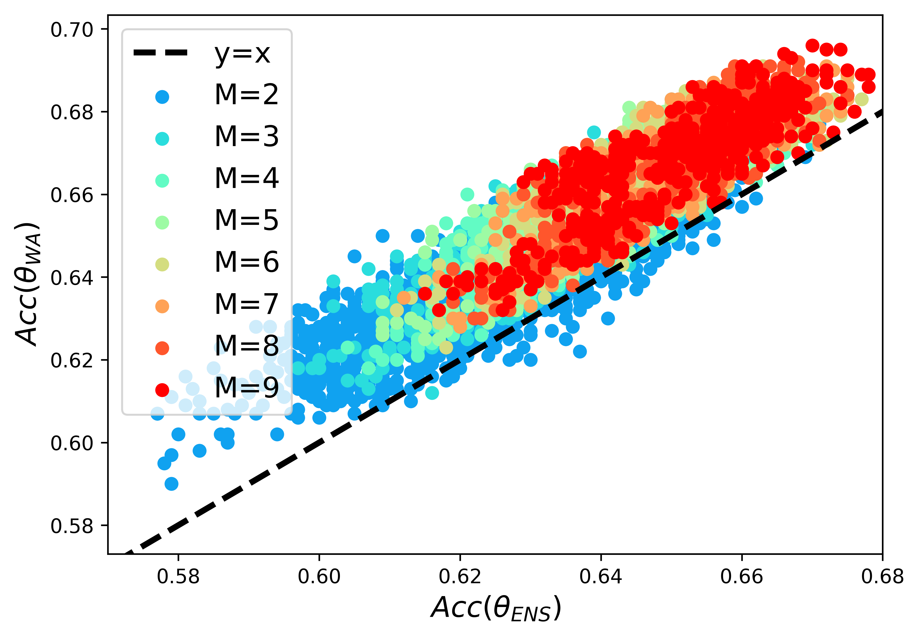
Figure 1 validates Lemma 1 and that $f_{\text{WA}}\approx f_{\text{ENS}}$. More precisely, $f_{\text{WA}}$ slightly but consistently improves $f_{\text{ENS}}$: we discuss this in Appendix D. Moreover, a larger $M$ improves the results; in accordance with Equation BVCL, this motivates averaging as many weights as possible. In contrast, large $M$ is computationally impractical for ENS at test time, requiring $M$ forwards.

Diversity and accuracy.

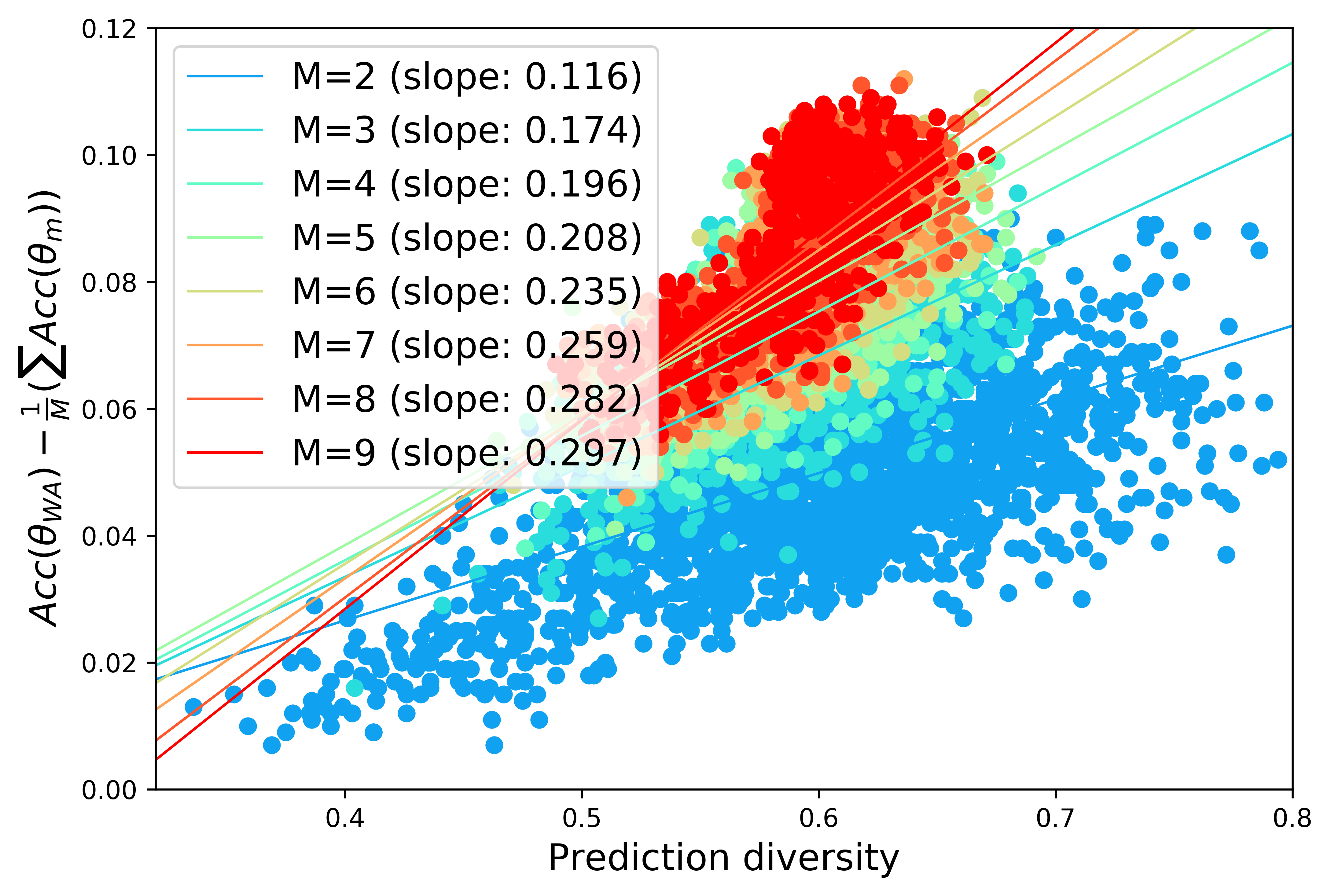
We validate in Figure 2 that $f_{\text{WA}}$ benefits from diversity. Here, we measure diversity with the ratio-error [46], i.e., the ratio $N_{\text{diff}}/N_{\text{simul}}$ between the number of different errors $N_{\text{diff}}$ and of simultaneous errors $N_{\text{simul}}$ in test for a pair in $\{f\mathopen{}\mathclose{{}\left(\cdot,\theta_{m}}\right)\}_{m=1}^{M}$. A higher average over the $\binom{M}{2}$ pairs means that members are less likely to err on the same inputs. Specifically, the gain of $\operatorname{Acc}(\theta_{\text{WA}})$ over the mean individual accuracy $\frac{1}{M}\sum_{m=1}^{M}\operatorname{Acc}\mathopen{}\mathclose{{}\left(\theta_{m}}\right)$ increases with diversity. Moreover, this phenomenon intensifies for larger $M$: the linear regression’s slope (i.e., the accuracy gain per unit of diversity) increases with $M$. This is consistent with the $(M-1)/M$ factor of $\mathrm{cov}\mathopen{}\mathclose{{}\left(x}\right)$ in Equation BVCL, as further highlighted in Section E.1.2. Finally, in Section E.1.1, we show that the conclusion also holds with CKAC [47], another established diversity measure.

Increasing diversity thus accuracy via different runs.

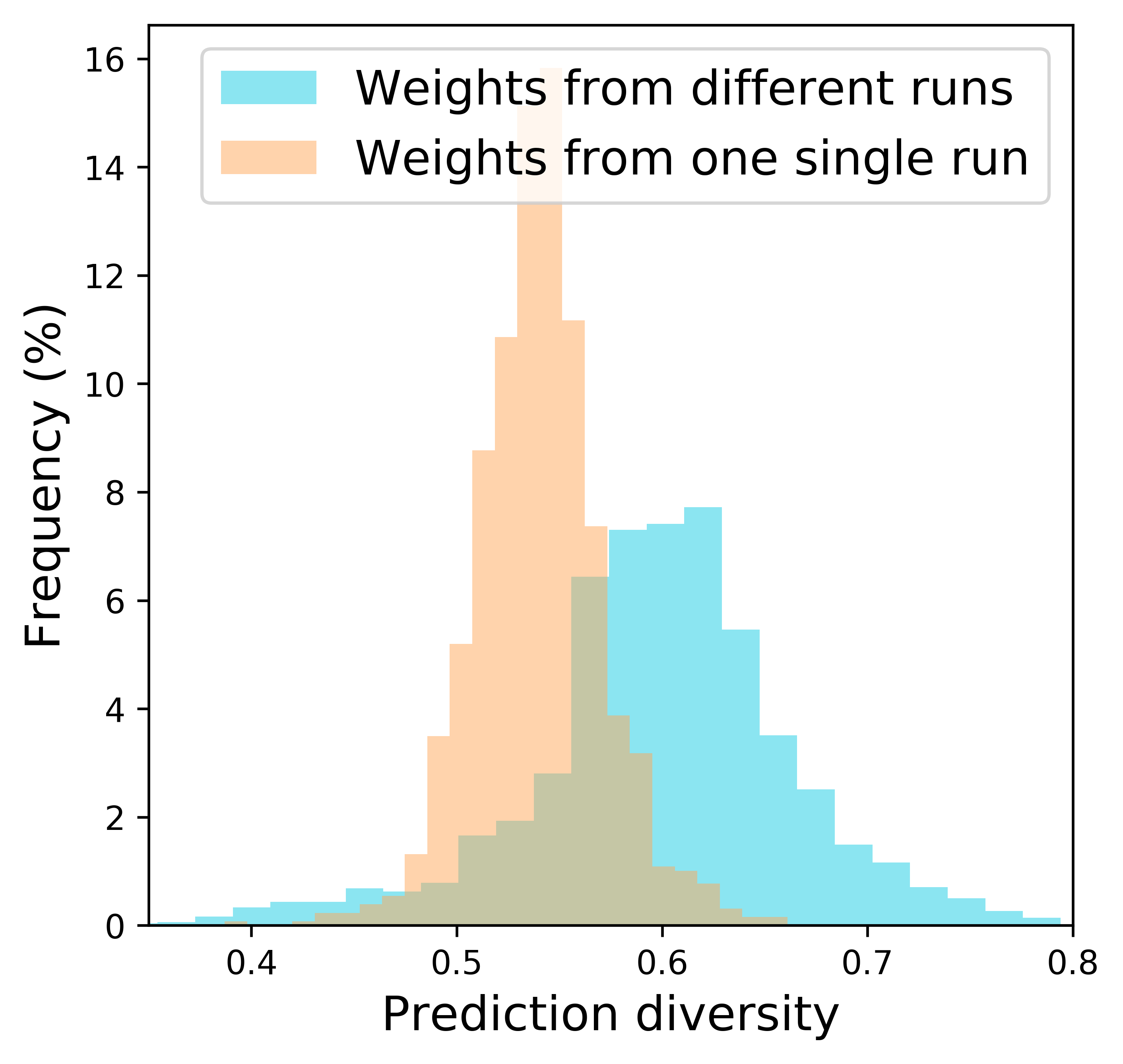
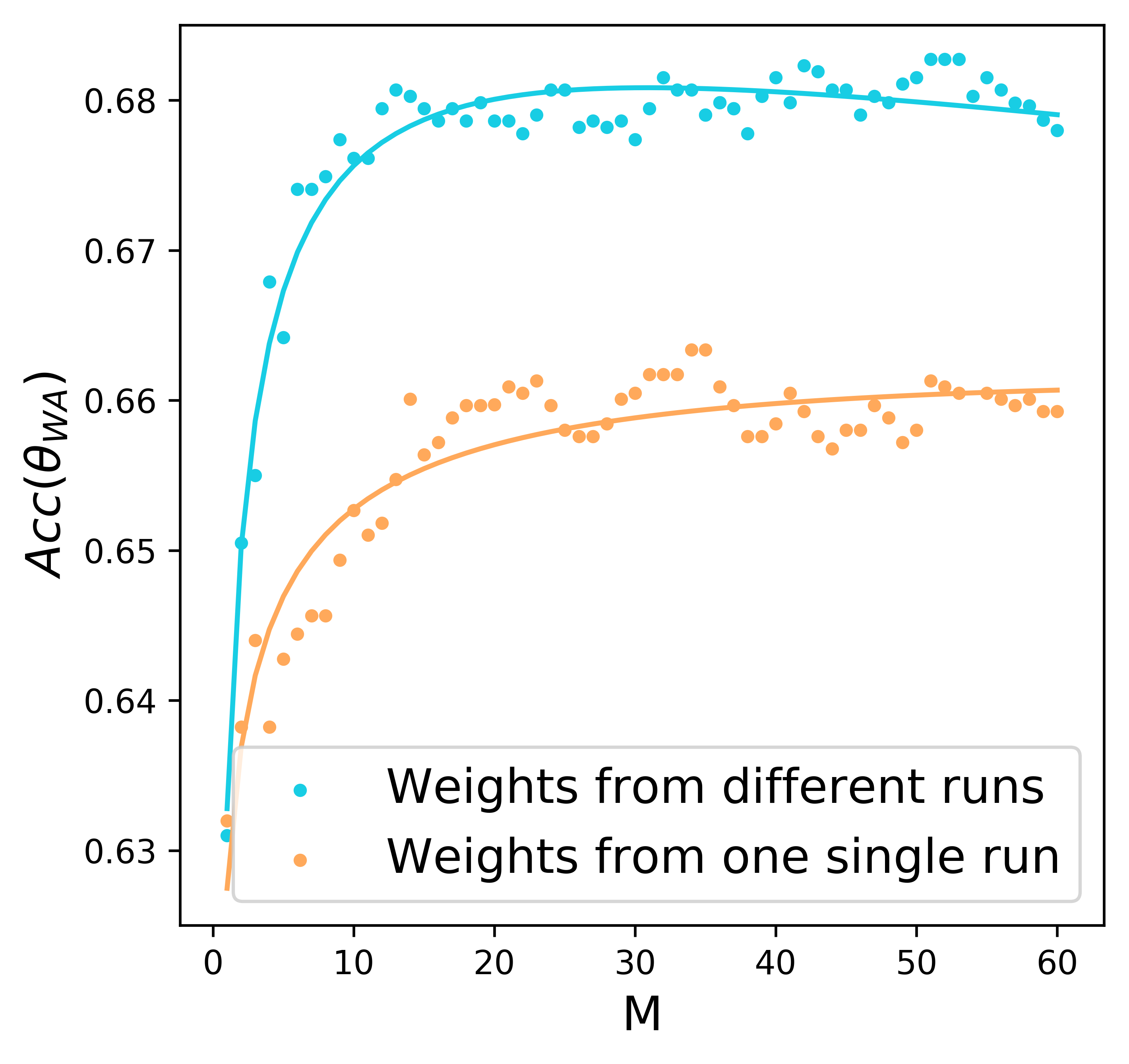
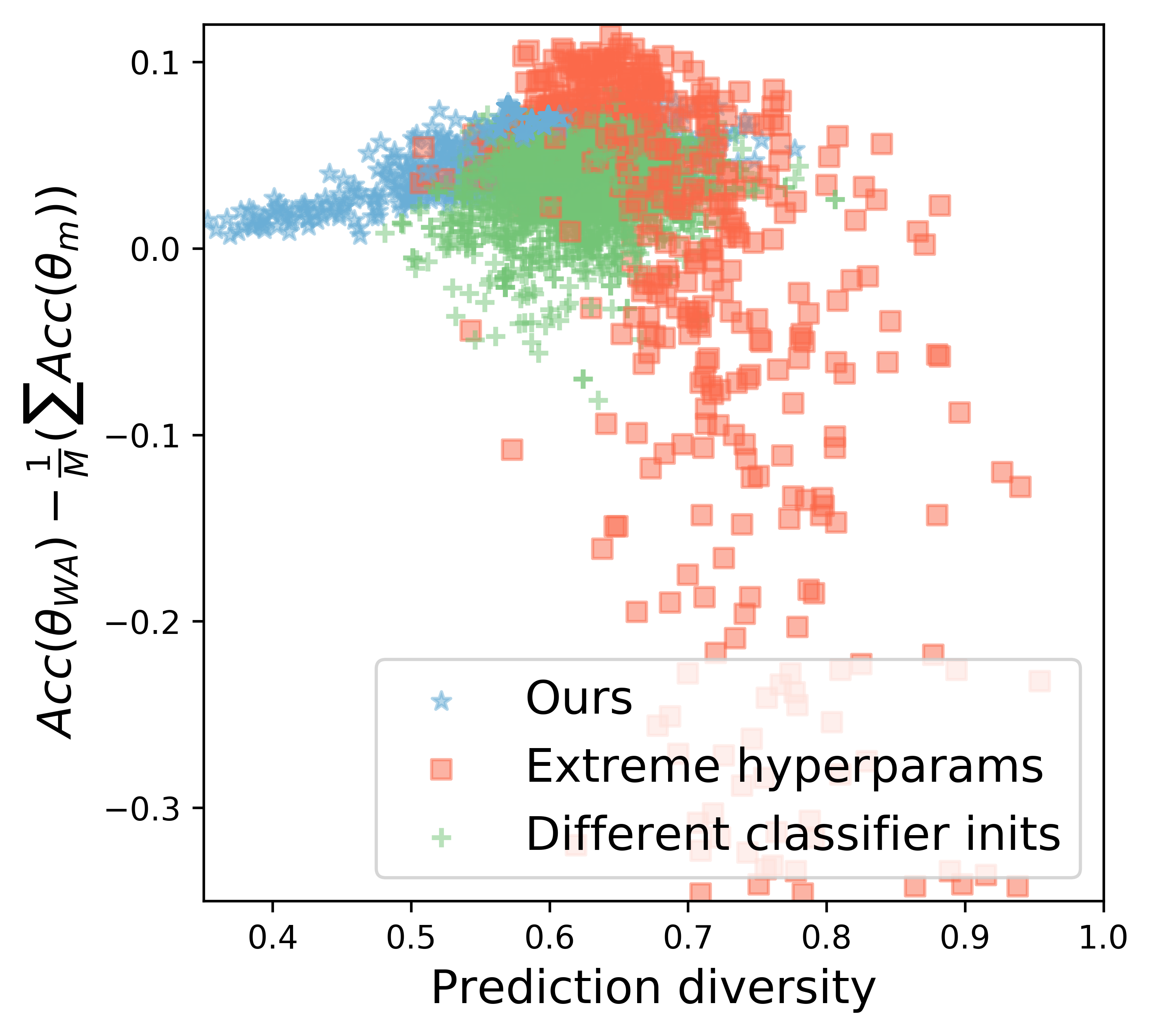
Now we investigate the difference between sampling the weights from a single run or from different runs. Figure 3 first shows that diversity increases when weights come from different runs. Second, in Figure 4, this is reflected on the accuracies in OOD. Here, we rank by validation accuracy the $60$ weights obtained (1) from $60$ different runs and (2) along $1$ well-performing run. We then consider the WA of the top $M$ weights as $M$ increases from $1$ to $60$. Both have initially the same performance and improve with $M$; yet, WA of weights from different runs gradually outperforms the single-run WA. Finally, Figure 5 shows that this holds only for mild hyperparameter ranges and with a shared initialization. Otherwise, when hyperparameter distributions are extreme (as defined in Table 7) or when classifiers are not similarly initialized, DiWA may perform worse than its members due to a violation of the locality condition. These experiments confirm that diversity is key as long as the weights remain averageable.

Figure 3: Frequencies of prediction diversities ($\uparrow$) [46] across $2$ weights obtained along a single run or from different runs.

Figure 4: WA accuracy ($\uparrow$) as $M$ increases, when the $M$ weights are obtained along a single run or from different runs.

Figure 5: Each dot displays the accuracy ($\uparrow$) gain of WA over its members vs. prediction diversity ($\uparrow$) for $2\leq M<10$ models.

5 Experimental results on the DomainBed benchmark

Datasets. We now present our evaluation on DomainBed [12]. By imposing the code, the training procedures and the ResNet50 [52] architecture, DomainBed is arguably the fairest benchmark for OOD generalization. It includes $5$ multi-domain real-world datasets: PACS [51], VLCS [53], OfficeHome [50], TerraIncognita [54] and DomainNet [55]. [19] showed that diversity shift dominates in these datasets. Each domain is successively considered as the target $T$ while other domains are merged into the source $S$. The validation dataset is sampled from $S$, i.e., we follow DomainBed’s training-domain model selection. The experimental setup is further described in Section G.1. Our code is available at https://github.com/alexrame/diwa.

Baselines. ERM is the standard Empirical Risk Minimization. Coral [10] is the best approach based on domain invariance. SWAD (Stochastic Weight Averaging Densely) [14] and MA (Moving Average) [29] average weights along one training trajectory but differ in their weight selection strategy. SWAD [14] is the current state of the art (SoTA) thanks to it “overfit-aware” strategy, yet at the cost of three additional hyperparameters (a patient parameter, an overfitting patient parameter and a tolerance rate) tuned per dataset. In contrast, MA [29] is easy to implement as it simply combines all checkpoints uniformly starting from batch $100$ until the end of training. Finally, we report the scores obtained in [29] for the costly Deep Ensembles (DENS) [15] (with different initializations): we discuss other ensembling strategies in Appendix D.

Our runs. ERM and DiWA share the same training protocol in DomainBed: yet, instead of keeping only one run from the grid-search, DiWA leverages $M$ runs. In practice, we sample $20$ configurations from the hyperparameter distributions detailed in Table 7 and report the mean and standard deviation across $3$ data splits. For each run, we select the weights of the epoch with the highest validation accuracy. ERM and MA select the model with highest validation accuracy across the $20$ runs, following standard practice on DomainBed. Ensembling (ENS) averages the predictions of all $M=20$ models (with shared initialization). DiWA-restricted selects $1\leq M\leq 20$ weights with Algorithm 1 while DiWA-uniform averages all $M=20$ weights. DiWA^† averages uniformly the $M=3\times 20=60$ weights from all $3$ data splits. DiWA^† benefits from larger $M$ (without additional inference cost) and from data diversity (see Section E.1.3). However, we cannot report standard deviations for DiWA^† for computational reasons. Moreover, DiWA^† cannot leverage the restricted weight selection, as the validation is not shared across all $60$ weights that have different data splits.

5.1 Results on DomainBed

We report our main results in Table 1, detailed per domain in Section G.2. With a randomly initialized classifier, DiWA^†-uniform is the best on PACS, VLCS and OfficeHome: DiWA-uniform is the second best on PACS and OfficeHome. On TerraIncognita and DomainNet, DiWA is penalized by some bad runs, filtered in DiWA-restricted which improves results on these datasets. Classifier initialization with linear probing (LP) [49] improves all methods on OfficeHome, TerraIncognita and DomainNet. On these datasets, DiWA^† increases MA by $1.3$, $0.5$ and $1.1$ points respectively. After averaging, DiWA^† with LP establishes a new SoTA of $68.0\%$, improving SWAD by $1.1$ points.

Table 1: Accuracy ($\%,\uparrow$) on DomainBed with ResNet50 (best in bold and second best underlined).

Algorithm Weight selection Init PACS VLCS OfficeHome TerraInc DomainNet Avg ERM N/A Random 85.5 $\pm$ 0.2 77.5 $\pm$ 0.4 66.5 $\pm$ 0.3 46.1 $\pm$ 1.8 40.9 $\pm$ 0.1 63.3 Coral [10] N/A 86.2 $\pm$ 0.3 78.8 $\pm$ 0.6 68.7 $\pm$ 0.3 47.6 $\pm$ 1.0 41.5 $\pm$ 0.1 64.6 SWAD [14] Overfit-aware 88.1 $\pm$ 0.1 79.1 $\pm$ 0.1 70.6 $\pm$ 0.2 50.0 $\pm$ 0.3 46.5 $\pm$ 0.1 66.9 MA [29] Uniform 87.5 $\pm$ 0.2 78.2 $\pm$ 0.2 70.6 $\pm$ 0.1 50.3 $\pm$ 0.5 46.0 $\pm$ 0.1 66.5 DENS [15, 29] Uniform: $M=6$ 87.6 78.5 70.8 49.2 47.7 66.8 Our runs ERM N/A Random 85.5 $\pm$ 0.5 77.6 $\pm$ 0.2 67.4 $\pm$ 0.6 48.3 $\pm$ 0.8 44.1 $\pm$ 0.1 64.6 MA [29] Uniform 87.9 $\pm$ 0.1 78.4 $\pm$ 0.1 70.3 $\pm$ 0.1 49.9 $\pm$ 0.2 46.4 $\pm$ 0.1 66.6 ENS Uniform: $M=20$ 88.0 $\pm$ 0.1 78.7 $\pm$ 0.1 70.5 $\pm$ 0.1 51.0 $\pm$ 0.5 47.4 $\pm$ 0.2 67.1 DiWA Restricted: $M\leq 20$ 87.9 $\pm$ 0.2 79.2 $\pm$ 0.1 70.5 $\pm$ 0.1 50.5 $\pm$ 0.5 46.7 $\pm$ 0.1 67.0 DiWA Uniform: $M=20$ 88.8 $\pm$ 0.4 79.1 $\pm$ 0.2 71.0 $\pm$ 0.1 48.9 $\pm$ 0.5 46.1 $\pm$ 0.1 66.8 DiWA^† Uniform: $M=60$ 89.0 79.4 71.6 49.0 46.3 67.1 ERM N/A LP [49] 85.9 $\pm$ 0.6 78.1 $\pm$ 0.5 69.4 $\pm$ 0.2 50.4 $\pm$ 1.8 44.3 $\pm$ 0.2 65.6 MA [29] Uniform 87.8 $\pm$ 0.3 78.5 $\pm$ 0.4 71.5 $\pm$ 0.3 51.4 $\pm$ 0.6 46.6 $\pm$ 0.0 67.1 ENS Uniform: $M=20$ 88.1 $\pm$ 0.3 78.5 $\pm$ 0.1 71.7 $\pm$ 0.1 50.8 $\pm$ 0.5 47.0 $\pm$ 0.2 67.2 DiWA Restricted: $M\leq 20$ 88.0 $\pm$ 0.3 78.5 $\pm$ 0.1 71.5 $\pm$ 0.2 51.6 $\pm$ 0.9 47.7 $\pm$ 0.1 67.5 DiWA Uniform: $M=20$ 88.7 $\pm$ 0.2 78.4 $\pm$ 0.2 72.1 $\pm$ 0.2 51.4 $\pm$ 0.6 47.4 $\pm$ 0.2 67.6 DiWA^† Uniform: $M=60$ 89.0 78.6 72.8 51.9 47.7 68.0

Table 2: Accuracy ($\%,\uparrow$) on OfficeHome domain “Art” with various objectives.

Algorithm No WA MA DiWA DiWA^† ERM 62.9 $\pm$ 1.3 65.0 $\pm$ 0.2 67.3 $\pm$ 0.2 67.7 Mixup 63.1 $\pm$ 0.7 66.2 $\pm$ 0.3 67.8 $\pm$ 0.6 68.4 Coral 64.4 $\pm$ 0.4 64.4 $\pm$ 0.4 67.7 $\pm$ 0.2 68.2 ERM/Mixup N/A N/A 67.9 $\pm$ 0.7 68.9 ERM/Coral N/A N/A 68.1 $\pm$ 0.3 68.7 ERM/Mixup/Coral N/A N/A 68.4 $\pm$ 0.4 69.1

DiWA with different objectives. So far we used ERM that does not leverage the domain information. Table 2 shows that DiWA-uniform benefits from averaging weights trained with Interdomain Mixup [56] and Coral [10]: accuracy gradually improves as we add more objectives. Indeed, as highlighted in Section E.1.3, DiWA benefits from the increased diversity brought by the various objectives. This suggests a new kind of linear connectivity across models trained with different objectives; the full analysis of this is left for future work.

5.2 Limitations of DiWA

Despite this success, DiWA has some limitations. First, DiWA cannot benefit from additional diversity that would break the linear connectivity between weights — as discussed in Appendix D. Second, DiWA (like all WA approaches) can tackle diversity shift but not correlation shift: this property is explained for the first time in Section 2.4 and illustrated in Appendix H on ColoredMNIST.

6 Related work

Generalization and ensemble. To generalize under distribution shifts, invariant approaches [8, 9, 11, 10, 57, 58] try to detect the causal mechanism rather than memorize correlations: yet, they do not outperform ERM on various benchmarks [12, 19, 59]. In contrast, ensembling of deep networks [15, 60, 61] consistently increases robustness [16] and was successfully applied to domain generalization [29, 62, 63, 64, 65, 66]. As highlighted in [18] (whose analysis underlies our Equation BVCL), ensembling works due to the diversity among its members. This diversity comes primarily from the randomness of the learning procedure [15] and can be increased with different hyperparameters [67], data [68, 69, 70], augmentations [71, 72] or with regularizations [65, 66, 73, 74].

Weight averaging. Recent works [13, 75, 76, 77] combine in weights (rather than in predictions) models collected along a single run. This was shown suboptimal in IID [17] but successful in OOD [14, 29]. Following the linear mode connectivity [24, 78] and the property that many independent models are connectable [79], a second group of works average weights with fewer constraints [26, 27, 28, 80, 81, 82]. To induce greater diversity, [83] used a high constant learning rate; [79] explicitly encouraged the weights to encompass more volume in the weight space; [82] minimized cosine similarity between weights; [84] used a tempered posterior. From a loss landscape perspective [20], these methods aimed at “explor[ing] the set of possible solutions instead of simply converging to a single point”, as stated in [83]. The recent “Model soups” introduced by Wortsman et al. [28] is a WA algorithm similar to Algorithm 1; yet, the theoretical analysis and the goals of these two works are different. Theoretically, we explain why WA succeeds under diversity shift: the bias/correlation shift, variance/diversity shift and diversity-based findings are novel and are confirmed empirically. Regarding the motivation, our work aims at combining more diverse weights: it may be analyzed as a general framework to average weights obtained in various ways. In contrast, [28] challenges the standard model selection after a grid search. Regarding the task, [28] and our work complement each other: while [28] demonstrate robustness on several ImageNet variants with distribution shift, we improve the SoTA on the multi-domain DomainBed benchmark against other established OOD methods after a thorough and fair comparison. Thus, DiWA and [28] are theoretically complementary with different motivations and applied successfully for different tasks.

7 Conclusion

In this paper, we propose a new explanation for the success of WA in OOD by leveraging its ensembling nature. Our analysis is based on a new bias-variance-covariance-locality decomposition for WA, where we theoretically relate bias to correlation shift and variance to diversity shift. It also shows that diversity is key to improve generalization. This motivates our DiWA approach that averages in weights models trained independently. DiWA improves the state of the art on DomainBed, the reference benchmark for OOD generalization. Critically, DiWA has no additional inference cost — removing a key limitation of standard ensembling. Our work may encourage the community to further create diverse learning procedures and objectives — whose models may be averaged in weights.

Acknowledgements

We would like to thank Jean-Yves Franceschi for his helpful comments and discussions on our paper. This work was granted access to the HPC resources of IDRIS under the allocation AD011011953 made by GENCI. We acknowledge the financial support by the French National Research Agency (ANR) in the chair VISA-DEEP (project number ANR-20-CHIA-0022-01) and the ANR projects DL4CLIM ANR-19-CHIA-0018-01, RAIMO ANR-20-CHIA-0021-01, OATMIL ANR-17-CE23-0012 and LEAUDS ANR-18-CE23-0020.

Checklist

1. For all authors…

   1. Do the main claims made in the abstract and introduction accurately reflect the paper’s contributions and scope? [Yes]

   2. Did you describe the limitations of your work? [Yes] In Section 5.2.

   3. Did you discuss any potential negative societal impacts of your work? [Yes] In Appendix A

   4. Have you read the ethics review guidelines and ensured that your paper conforms to them? [Yes]

2. If you are including theoretical results…

   1. Did you state the full set of assumptions of all theoretical results? [Yes] Assumption 1 discussed in Section C.3.2 and Assumptions 2 and 3 discussed in Section C.4.2.

   2. Did you include complete proofs of all theoretical results? [Yes] In Appendix C

3. If you ran experiments…

   1. Did you include the code, data, and instructions needed to reproduce the main experimental results (either in the supplemental material or as a URL)? [Yes] Our code is available at https://github.com/alexrame/diwa.

   2. Did you specify all the training details (e.g., data splits, hyperparameters, how they were chosen)? [Yes] See Section 5 and Section G.1

   3. Did you report error bars (e.g., with respect to the random seed after running experiments multiple times)? [Yes] Defined by different data splits when possible.

   4. Did you include the total amount of compute and the type of resources used (e.g., type of GPUs, internal cluster, or cloud provider)? [Yes] Approximately $20000$ hours of GPUs (Nvidia V100) on an internal cluster, mostly for the $2640$ runs needed in Table 1.

4. If you are using existing assets (e.g., code, data, models) or curating/releasing new assets…

   1. If your work uses existing assets, did you cite the creators? [Yes] DomainBed benchmark [12] and its datasets.

   2. Did you mention the license of the assets? [Yes] DomainBed is under “The MIT License”.

   3. Did you include any new assets either in the supplemental material or as a URL? [No]

   4. Did you discuss whether and how consent was obtained from people whose data you’re using/curating? [N/A]

   5. Did you discuss whether the data you are using/curating contains personally identifiable information or offensive content? [N/A]

5. If you used crowdsourcing or conducted research with human subjects…

   1. Did you include the full text of instructions given to participants and screenshots, if applicable? [N/A]

   2. Did you describe any potential participant risks, with links to Institutional Review Board (IRB) approvals, if applicable? [N/A]

   3. Did you include the estimated hourly wage paid to participants and the total amount spent on participant compensation? [N/A]

This supplementary material complements the main paper. It is organized as follows:

1. Appendix A describes the broader impact of our work.

2. Appendix B points out the limitations of existing flatness-based analysis of WA and shows how our analysis solves these limitations.

3. Appendix C details all the proofs of the propositions and lemmas found in our work.

   • Sections C.1 and 1 derive the bias-variance-covariance-locality decomposition for WA (Proposition 1).

   • Section C.3 establishes the link between bias and correlation shift (Proposition 2).

   • Section C.4 establishes the link between variance and diversity shift (Proposition 3).

   • Section C.5 compares WA with one of its member (Lemma 3).

4. Appendix D empirically compares WA to functional ensembling ENS.

5. Appendix E presents some additional diversity results on OfficeHome and PACS.

6. Appendix F ablates the importance of the number of training runs.

7. Appendix G describes our experiments on DomainBed and our per-domain results.

8. Appendix H empirically confirms a limitation of WA approaches expected from our theoretical analysis: they do not tackle correlation shift on ColoredMNIST.

9. Appendix I suggests DiWA’s potential when some target data is available for training [85].

Appendix A Broader impact statement

We believe our paper can have several positive impacts. First, our theoretical analysis enables practitioners to know when averaging strategies succeed (under diversity shift, where variance dominates) or break down (under correlation shift, where bias dominates). This is key to understand when several models can be combined into a production system, or if the focus should be put on the training objective and/or the data. Second, it sets a new state of the art for OOD generalization under diversity shift without relying on a specific objective, architecture or task prior. It could be useful in medicine [1, 2] or to tackle fairness issues related to under-representation [57, 86, 87]. Finally, DIWA has no additional inference cost; in contrast, functional ensembling needs one forward per member. Thus, DiWA removes the carbon footprint overhead of ensembling strategies at test-time.

Yet, our paper may also have some negative impacts. First, it requires independent training of several models. It may motivate practitioners to learn even more networks and average them afterwards. Note that in Section 5, we restricted ourselves to combining only the runs obtained from the standard ERM grid search from DomainBed [12]. Second, our model is fully deep learning based with the corresponding risks, e.g., adversarial attacks and lack of interpretability. Finally, we do not control its possible use to surveillance or weapon systems.

Appendix B Limitations of the flatness-based analysis in OOD

Theorem 1 (Equation 21 from [14], simplified version of their Theorem 1).

Consider a set of $N$ covers $\mathopen{}\mathclose{{}\left\{\Theta_{k}}\right\}_{k=1}^{N}$ s.t. the parameter space $\Theta\subset\cup_{k}^{N}\Theta_{k}$ where $\operatorname{diam}(\Theta)\triangleq\sup_{\theta,\theta^{\prime}\in\Theta}\mathopen{}\mathclose{{}\left\|\theta-\theta^{\prime}}\right\|_{2},N\triangleq\mathopen{}\mathclose{{}\left\lceil(\operatorname{diam}(\Theta)/\gamma)^{d}}\right\rceil$ and $d$ is the dimension of $\Theta$. Then, $\forall\theta\in\Theta$ with probability at least $1-\delta$:

$$\mathcal{E}_{T}(\theta) \leq\frac{1}{2}\operatorname{Div}(p_{S},p_{T})+\mathcal{E}_{S}(\theta)$$ (5)

$$\leq\frac{1}{2}\operatorname{Div}(p_{S},p_{T})+\mathcal{E}_{d_{S}}^{\gamma}(\theta)+\max_{k}\sqrt{\frac{\mathopen{}\mathclose{{}\left(v_{k}\mathopen{}\mathclose{{}\left[\ln\mathopen{}\mathclose{{}\left(n_{S}/v_{k}}\right)+1}\right]+\ln(N/\delta)}\right)}{2n_{S}}},$$

where:

• $\mathcal{E}_{T}(\theta)\triangleq\mathbb{E}_{(x,y)\sim p_{T}(X,Y)}[\ell\mathopen{}\mathclose{{}\left(f_{\theta}(x);y}\right)]$ is the expected risk on the target domain,

• $\operatorname{Div}(p_{S},p_{T})\triangleq 2\sup_{A}\mathopen{}\mathclose{{}\left|p_{S}(A)-p_{T}(A)}\right|$ is a divergence between the source and target marginal distributions $p_{S}$ and $p_{T}$: it measures diversity shift.

• $\mathcal{E}_{S}(\theta)\triangleq\mathbb{E}_{(x,y)\sim p_{S}(X,Y)}[\ell\mathopen{}\mathclose{{}\left(f_{\theta}(x);y}\right)]$ is the expected risk on the source domain,

• $\mathcal{E}_{d_{S}}^{\gamma}(\theta)\triangleq\max_{\|\Delta\|\leq\gamma}\mathcal{E}_{d_{S}}(\theta+\Delta)$ (where $\mathcal{E}_{d_{S}}(\theta+\Delta)\triangleq\mathbb{E}_{(x,y)\in d_{S}}[\ell\mathopen{}\mathclose{{}\left(f_{\theta+\Delta}(x);y}\right)]$) is the robust empirical loss on source training dataset $d_{S}$ from $S$ of size $n_{S}$,

• $v_{k}$ is a VC dimension of each $\Theta_{k}$.

Previous understanding of WA’s success in OOD relied on this upper-bound, where $\mathcal{E}_{d_{S}}^{\gamma}(\theta)$ involves the solution’s flatness. This is usually empirically analyzed by the trace of the Hessian [88, 89, 90]: indeed, with a second-order Taylor approximation around the local minima $\theta$ and $h$ the Hessian’s maximum eigenvalue, $\mathcal{E}_{d_{S}}^{\gamma}(\theta)\approx\mathcal{E}_{d_{S}}(\theta)+h\times\gamma^{2}$.

In the following subsections, we show that this inequality does not fully explain the exceptional performance of WA on DomainBed [12]. Moreover, we illustrate that our bias-variance-covariance-locality addresses these limitations.

B.1 Flatness does not act on distribution shifts

The flatness-based analysis is not specific to OOD. Indeed, the upper-bound in Equation 5 sums up two noninteracting terms: a domain divergence $\mathrm{Div}(p_{S},p_{T})$ that grows in OOD and $\mathcal{E}_{d_{S}}^{\gamma}(\theta)$ that measures the IID flatness. The flatness term can indeed be reduced empirically with WA: yet, it does not tackle the domain gap. In fact, Equation 5 states that additional flatness reduces the upper bound of the error similarly no matter the strength of the distribution shift, thus as well OOD than IID. In contrast, our analysis shows that variance (which grows with diversity shift, see Section 2.4.2) is tackled for large $M$: our error is controlled even under large diversity shift. This is consistent with our experiments in Table 1. Our analysis also explains why WA cannot tackle correlation shift (where bias dominates, see Appendix H), a limitation [14] does not illustrate.

B.2 SAM leads to flatter minimas but worse OOD performance

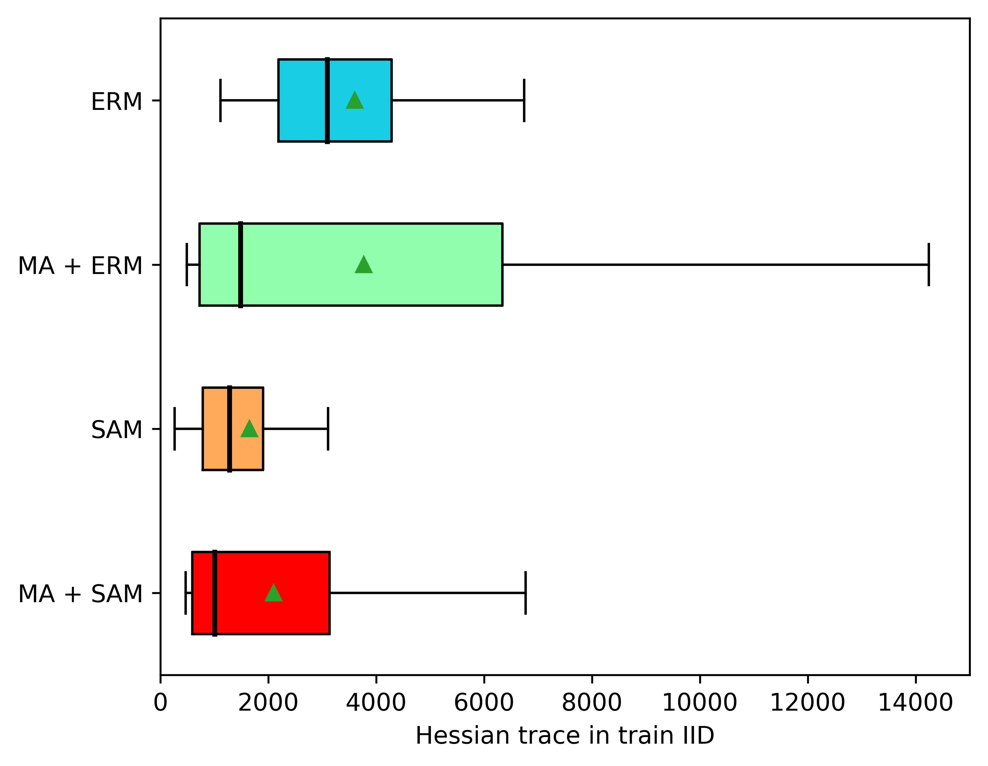
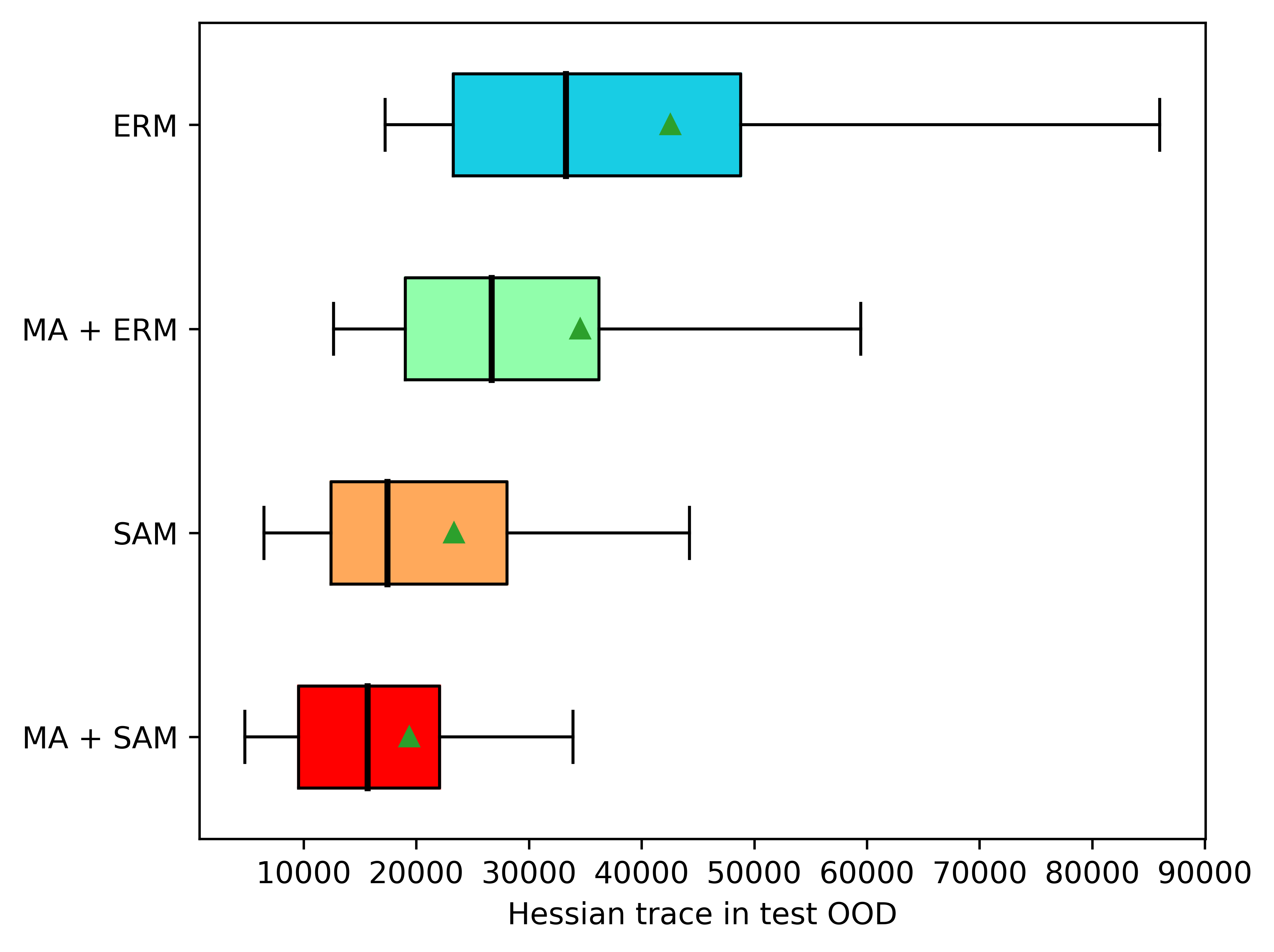
The flatness-based analysis does not explain why WA outperforms other flatness-based methods in OOD. We consider Sharpness-Aware Minimizer (SAM) [30], another popular method to find flat minima based on minimax optimization: it minimizes the maximum loss around a neighborhood of the current weights $\theta$. In Figure 6, we compare the flatness (i.e., the Hessian trace computed with the package in [90]) and accuracy of ERM, MA [29] (a WA strategy) and SAM [30] when trained on the “Clipart”, “Product” and “Photo” domains from OfficeHome [50]: they are tested OOD on the fourth domain “Art”. Analyzing the second and the third rows of Figures 6(a) and 6(b), we observe that SAM indeed finds flat minimas (at least comparable to MA), both in training (IID) and test (OOD). However, this is not reflected in the OOD accuracies in Figure 6(c), where MA outperforms SAM. As reported in Table 3, similar experiments across more datasets lead to the same conclusions in [14]. In conclusion, flatness is not sufficient to explain why WA works so well in OOD, because SAM has similar flatness but worse OOD results. In contrast, we highlight in this paper that WA succeeds in OOD by reducing the impact of variance thanks to its similarity with prediction ensembling [15] (see Lemma 1), a privileged link that SAM does not benefit from.

Table 3: Accuracy ($\uparrow$) on DomainBed for SWAD, taken from Table 4 in [14]

PACS VLCS OfficeHome TerraInc DomainNet Avg. ( $\Delta)$ ERM 85.5 $\pm$ 0.2 77.5 $\pm$ 0.4 66.5 $\pm$ 0.3 46.1 $\pm$ 1.8 40.9 $\pm$ 0.1 63.3 SWAD [14] + ERM 88.1 $\pm$ 0.1 79.1 $\pm$ 0.1 70.6 $\pm$ 0.2 50.0 $\pm$ 0.3 46.5 $\pm$ 0.1 66.9(+3.6) SAM [30] 85.8 $\pm$ 0.2 79.4 $\pm$ 0.1 69.6 $\pm$ 0.1 43.3 $\pm$ 0.7 44.3 $\pm$ 0.0 64.5 SWAD [14] + SAM [30] 87.1 $\pm$ 0.2 78.5 $\pm$ 0.2 69.9 $\pm$ 0.1 45.3 $\pm$ 0.9 46.5 $\pm$ 0.1 65.5(+1.0)

(a) Hessian trace ($\downarrow$) in train.

(b) Hessian trace ($\downarrow$) in test OOD.

(c) Accuracy ($\uparrow$) in test OOD.

Figure 6: MA [29] (a WA strategy) and SAM [30] similarly improve flatness. When combined, they further improve flatness. Yet, MA outperforms SAM and beats MA + SAM in OOD accuracy on domain “Art” from OfficeHome.

Table 4: Accuracy ($\uparrow$) impact of including SAM on domain “Art” from OfficeHome.

Algorithm Weight selection ERM SAM [30] No DiWA N/A 62.9 $\pm$ 1.3 63.5 $\pm$ 0.5 DiWA Restricted: $M\leq 20$ 66.7 $\pm$ 0.1 65.4 $\pm$ 0.1 DiWA Uniform: $M=20$ 67.3 $\pm$ 0.3 66.7 $\pm$ 0.2 DiWA^† Uniform: $M=60$ 67.7 67.4

B.3 WA and SAM are not complementary in OOD when variance dominates

Figure 7: Prediction diversity in ratio-error [46] ($\uparrow$) on domain “Art” from OfficeHome. Checkpoints along a SAM run are less diverse than along an ERM run.

We investigate a similar inconsistency when combining these two flatness-based methods. As argued in [31], we confirm in Figures 6(a) and 6(b) that MA + SAM leads to flatter minimas than MA alone (i.e., with ERM) or SAM alone. Yet, MA does not benefit from SAM in Figure 6(c). [14] showed an even stronger result in Table 3: SWAD + ERM performs better than SWAD + SAM. We recover similar findings in Table 4: DiWA performs worse when SAM is applied in each training run.

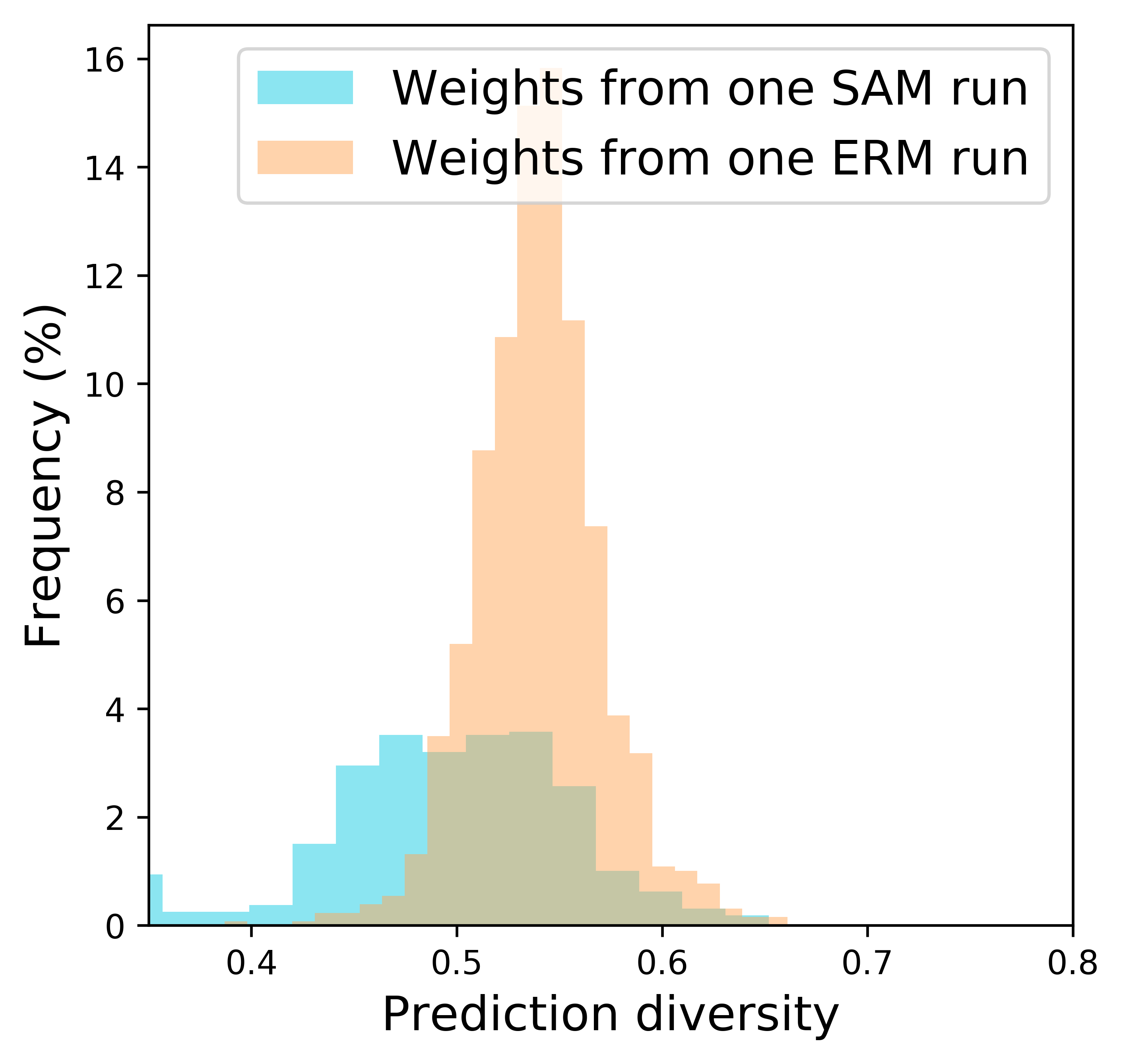
This behavior is not explained by Theorem 1, which states that more flatness should improve OOD generalization. Yet it is explained by our diversity-based analysis. Indeed, we observe in Figure 7 that the diversity across two checkpoints along a SAM trajectory is much lower than along a standard ERM trajectory (with SGD). We speculate that this is related to the recent empirical observation made in [91]: “the rank of the CLIP representation space is drastically reduced when training CLIP with SAM”. Under diversity shift, variance dominates (see Equation 4): in this setup, the gain in accuracy of models trained with SAM cannot compensate the decrease in diversity. This explains why WA and SAM are not complementary under diversity shift: in this case, variance is large.

Appendix C Proofs

C.1 WA loss derivation

Lemma (1).

Given $\{\theta_{m}\}_{m=1}^{M}$ with learning procedures $L_{S}^{M}\triangleq\{l_{S}^{(m)}\}_{m=1}^{M}$. Denoting $\Delta_{L_{S}^{M}}=\max_{m=1}^{M}\mathopen{}\mathclose{{}\left\|\theta_{m}-\theta_{\text{WA}}}\right\|_{2}$, $\forall(x,y)\in\mathcal{X}\times\mathcal{Y}$:

$$f_{\text{WA}}(x)=f_{\text{ENS}}(x)+O(\Delta^{2}_{L_{S}^{M}})\text{~{}and~{}}\ell\mathopen{}\mathclose{{}\left(f_{\text{WA}}(x),y}\right)=\ell\mathopen{}\mathclose{{}\left(f_{\text{ENS}}(x),y}\right)+O(\Delta_{L_{S}^{M}}^{2}).$$

Proof.

This proof has two components:

• to establish the functional approximation, as [13], it performs Taylor expansion of the models’ predictions at the first order.

• to establish the loss approximation, as [28], it performs Taylor expansion of the loss at the first order.

Functional approximation

With a Taylor expansion at the first order of the models’ predictions w.r.t. parameters $\theta$:

$$f_{\theta_{m}} =f_{\text{WA}}+\nabla f_{\text{WA}}^{\intercal}\Delta_{m}+O\mathopen{}\mathclose{{}\left(\mathopen{}\mathclose{{}\left\|\Delta_{m}}\right\|_{2}^{2}}\right)$$

$$f_{\text{ENS}}-f_{\text{WA}} =\frac{1}{M}\sum_{m=1}^{M}\mathopen{}\mathclose{{}\left(\nabla f_{\text{WA}}^{\intercal}\Delta_{m}+O\mathopen{}\mathclose{{}\left(\mathopen{}\mathclose{{}\left\|\Delta_{m}}\right\|_{2}^{2}}\right)}\right)$$

Therefore, because $\sum_{m=1}^{M}\Delta_{m}=0$,

$$f_{\text{ENS}}-f_{\text{WA}}=O\mathopen{}\mathclose{{}\left(\Delta^{2}}\right)\text{~{}where~{}}\Delta=\max_{m=1}^{M}\mathopen{}\mathclose{{}\left\|\Delta_{m}}\right\|_{2}.$$ (6)

Loss approximation

With a Taylor expansion at the zeroth order of the loss w.r.t. its first input and injecting Equation 6:

$$\ell\mathopen{}\mathclose{{}\left(f_{\text{ENS}}(x);y}\right) =\ell\mathopen{}\mathclose{{}\left(f_{\text{WA}}(x);y}\right)+O\mathopen{}\mathclose{{}\left(\mathopen{}\mathclose{{}\left\|f_{\text{ENS}}(x)-f_{\text{WA}}(x)}\right\|_{2}}\right)$$

$$\ell\mathopen{}\mathclose{{}\left(f_{\text{ENS}}(x);y}\right) =\ell\mathopen{}\mathclose{{}\left(f_{\text{WA}}(x);y}\right)+O\mathopen{}\mathclose{{}\left(\Delta^{2}}\right).$$

∎

C.2 Bias-variance-covariance-locality decomposition

Remark 1.

Our result in Proposition 1 is simplified by leveraging the fact that the learning procedures $L_{S}^{M}=\{l_{S}^{(m)}\}_{m=1}^{M}$ are identically distributed (i.d.). This assumption naturally holds for DiWA which selects weights from different runs with i.i.d. hyperparameters. It may be less obvious why it applies to MA [29] and SWAD [14]. It is even false if the weights $\{\theta(l_{S}^{(m)})\}_{m=1}^{M}$ are defined as being taken sequentially along a training trajectory, i.e., when $0\leq i<j\leq M$ implies that $l_{S}^{(i)}$ has fewer training steps than $l_{S}^{(j)}$. We propose an alternative indexing strategy to respect the i.d. assumption. Given $M$ weights selected by the weight selection procedure, we draw without replacement the $M$ weights, i.e., $\theta(l_{S}^{(i)})$ refers to the $i^{th}$ sampled weights. With this procedure, all weights are i.d. as they are uniformly sampled. Critically, their WA are unchanged for the two definitions.

Proposition (1).

Denoting $\bar{f}_{S}\mathopen{}\mathclose{{}\left(x}\right)=\mathbb{E}_{l_{S}}\mathopen{}\mathclose{{}\left[f\mathopen{}\mathclose{{}\left(x,\theta\mathopen{}\mathclose{{}\left(l_{S}}\right)}\right)}\right]$, under identically distributed learning procedures $L_{S}^{M}\triangleq\{l_{S}^{(m)}\}_{m=1}^{M}$, the expected generalization error on domain $T$ of $\theta_{\text{WA}}(L_{S}^{M})\triangleq\frac{1}{M}\sum\nolimits_{m=1}^{M}\theta_{m}$ over the joint distribution of $L_{S}^{M}$ is:

$$\mathbb{E}_{L_{S}^{M}}\mathcal{E}_{T}(\theta_{\text{WA}}(L_{S}^{M})) =\mathbb{E}_{(x,y)\sim p_{T}}\Big{[}\mathrm{bias}^{2}(x,y)+\frac{1}{M}\mathrm{var}(x)+\frac{M-1}{M}\mathrm{cov}(x)\Big{]}+O(\bar{\Delta}^{2}),$$ (BVCL)

$$\text{where~{}}\mathrm{bias}(x,y) =y-\bar{f}_{S}\mathopen{}\mathclose{{}\left(x}\right),$$

$$\text{and~{}}\mathrm{var}(x) =\mathbb{E}_{l_{S}}\mathopen{}\mathclose{{}\left[\mathopen{}\mathclose{{}\left(f(x,\theta(l_{S}))-\bar{f}_{S}\mathopen{}\mathclose{{}\left(x}\right)}\right)^{2}}\right],$$

$$\text{and~{}}\mathrm{cov}(x) =\mathbb{E}_{l_{S},l_{S}^{\prime}}\mathopen{}\mathclose{{}\left[\mathopen{}\mathclose{{}\left(f(x,\theta(l_{S}))-\bar{f}_{S}\mathopen{}\mathclose{{}\left(x}\right)}\right)\mathopen{}\mathclose{{}\left(f(x,\theta(l_{S}^{\prime})))-\bar{f}_{S}\mathopen{}\mathclose{{}\left(x}\right)}\right)}\right],$$

$$\text{and~{}}\bar{\Delta}^{2} =\mathbb{E}_{L_{S}^{M}}\Delta_{L_{S}^{M}}^{2}\text{~{}with~{}}\Delta_{L_{S}^{M}}=\max_{m=1}^{M}\mathopen{}\mathclose{{}\left\|\theta_{m}-\theta_{\text{WA}}}\right\|_{2}.$$

$\mathrm{cov}$ is the prediction covariance between two member models whose weights are averaged. The locality term $\bar{\Delta}^{2}$ is the expected squared maximum distance between weights and their average.

Proof.

This proof has two components:

• it follows the bias-variance-covariance decomposition from [18, 35] for functional ensembling. It is tailored to WA by assuming that learning procedures are identically distributed.

• it injects the obtained equation into Lemma 1 to obtain the Proposition 1 for WA.

BVC for ensembling with identically distributed learning procedures

With $\bar{f}_{S}\mathopen{}\mathclose{{}\left(x}\right)=\mathbb{E}_{l_{S}}\mathopen{}\mathclose{{}\left[f\mathopen{}\mathclose{{}\left(x,\theta\mathopen{}\mathclose{{}\left(l_{S}}\right)}\right)}\right]$, we recall the bias-variance decomposition [32] (Equation BV):

$$\mathbb{E}_{l_{S}}\mathcal{E}_{T}(\theta(l_{S})) =\mathbb{E}_{(x,y)\sim p_{T}}\Big{[}\mathrm{bias}(x,y)^{2}+\mathrm{var}(x)\Big{]},$$

$$\text{where~{}}\mathrm{bias}(x,y) =\operatorname{Bias}\{f|(x,y)\}=y-\bar{f}_{S}\mathopen{}\mathclose{{}\left(x}\right),$$

$$\text{and~{}}\mathrm{var}(x) =\operatorname{Var}\{f|x\}=\mathbb{E}_{l_{S}}\mathopen{}\mathclose{{}\left[\mathopen{}\mathclose{{}\left(f(x,\theta(l_{S}))-\bar{f}_{S}\mathopen{}\mathclose{{}\left(x}\right)}\right)^{2}}\right].$$

Using $f_{\text{ENS}}\triangleq f_{\text{ENS}}(\cdot,\{\theta(l_{S}^{(m)})\}_{m=1}^{M})\triangleq\frac{1}{M}\sum_{m=1}^{M}f(\cdot,\theta(l_{S}^{(m)}))$ in this decomposition yields,

$$\mathbb{E}_{L_{S}^{M}}\mathcal{E}_{T}(\{\theta(l_{S}^{(m)})\}_{m=1}^{M})=\mathbb{E}_{x\sim p_{T}}\mathopen{}\mathclose{{}\left[\operatorname{Bias}\mathopen{}\mathclose{{}\left\{f_{\text{ENS}}\mid(x,y)}\right\}^{2}+\operatorname{Var}\mathopen{}\mathclose{{}\left\{f_{\text{ENS}}\mid x}\right\}}\right].$$ (7)

As $f_{\text{ENS}}$ depends on $L_{S}^{M}$, we extend the bias into:

$$\operatorname{Bias}\mathopen{}\mathclose{{}\left\{f_{\text{ENS}}\mid(x,y)}\right\} =y-\mathbb{E}_{L_{S}^{M}}\mathopen{}\mathclose{{}\left[\frac{1}{M}\sum_{m=1}^{M}f(x,\theta(l_{S}^{(m)}))}\right]=y-\frac{1}{M}\sum_{m=1}^{M}\mathbb{E}_{l_{S}^{(m)}}\mathopen{}\mathclose{{}\left[f(x,\theta(l_{S}^{(m)}))}\right]$$

Under identically distributed $L_{S}^{M}\triangleq\{l_{S}^{(m)}\}_{m=1}^{M}$,

$$\frac{1}{M}\sum_{m=1}^{M}\mathbb{E}_{l_{S}^{(m)}}\mathopen{}\mathclose{{}\left[y-f(x,\theta(l_{S}^{(m)}))}\right]=\mathbb{E}_{l_{S}}\mathopen{}\mathclose{{}\left[y-f(x,\theta(l_{S}))}\right]=\operatorname{Bias}\{f|(x,y)\}.$$

Thus the bias of ENS is the same as for a single member of the WA.

Regarding the variance:

$$\operatorname{Var}\mathopen{}\mathclose{{}\left\{f_{\text{ENS}}\mid x}\right\}=\mathbb{E}_{L_{S}^{M}}\mathopen{}\mathclose{{}\left[\mathopen{}\mathclose{{}\left(\frac{1}{M}\sum_{m=1}^{M}f(x,\theta(l_{S}^{(m)}))-\mathbb{E}_{L_{S}^{M}}\mathopen{}\mathclose{{}\left[\frac{1}{M}\sum_{m=1}^{M}f(x,\theta(l_{S}^{(m)}))}\right]}\right)^{2}}\right].$$

Under identically distributed $L_{S}^{M}\triangleq\{l_{S}^{(m)}\}_{m=1}^{M}$,

$$\operatorname{Var}\mathopen{}\mathclose{{}\left\{f_{\text{ENS}}\mid x}\right\}=\frac{1}{M^{2}}\sum_{m=1}^{M}\mathbb{E}_{l_{S}}\mathopen{}\mathclose{{}\left[\mathopen{}\mathclose{{}\left(f(x,\theta(l_{S}))-\mathbb{E}_{l_{S}}\mathopen{}\mathclose{{}\left[f(x,\theta(l_{S}))}\right]}\right)^{2}}\right]+$$

$$\quad\quad\quad\quad\frac{1}{M^{2}}\sum_{m}\sum_{m^{\prime}\neq m}\mathbb{E}_{l_{S},l_{S}^{\prime}}\mathopen{}\mathclose{{}\left[\mathopen{}\mathclose{{}\left(f(x,\theta(l_{S}))-\mathbb{E}_{l_{S}}\mathopen{}\mathclose{{}\left[f(x,\theta(l_{S}))}\right]}\right)\mathopen{}\mathclose{{}\left(f(x,\theta(l_{S}^{\prime}))-\mathbb{E}_{l_{S}^{\prime}}\mathopen{}\mathclose{{}\left[f(x,\theta(l_{S}^{\prime}))}\right]}\right)}\right]$$

$$=\frac{1}{M}\mathbb{E}_{l_{S}}\mathopen{}\mathclose{{}\left[\mathopen{}\mathclose{{}\left(f(x,\theta(l_{S}))-\mathbb{E}_{l_{S}}\mathopen{}\mathclose{{}\left[f(x,\theta(l_{S}))}\right]}\right)^{2}}\right]+$$

$$\quad\quad\quad\quad\frac{M-1}{M}\mathbb{E}_{l_{S},l_{S}^{\prime}}\mathopen{}\mathclose{{}\left[\mathopen{}\mathclose{{}\left(f(x,\theta(l_{S}))-\mathbb{E}_{l_{S}}\mathopen{}\mathclose{{}\left[f(x,\theta(l_{S}))}\right]}\right)\mathopen{}\mathclose{{}\left(f(x,\theta(l_{S}^{\prime}))-\mathbb{E}_{l_{S}^{\prime}}\mathopen{}\mathclose{{}\left[f(x,\theta(l_{S}^{\prime}))}\right]}\right)}\right]$$

$$=\frac{1}{M}\mathrm{var}\mathopen{}\mathclose{{}\left(x}\right)+\mathopen{}\mathclose{{}\left(1-\frac{1}{M}}\right)\mathrm{cov}\mathopen{}\mathclose{{}\left(x}\right).$$

The variance is split into the variance of a single member (divided by $M$) and a covariance term.

Combination with Lemma 1

We recall that per Lemma 1,

$$\ell\mathopen{}\mathclose{{}\left(f_{\text{WA}}(x),y}\right)=\ell\mathopen{}\mathclose{{}\left(f_{\text{ENS}}(x),y}\right)+O(\Delta_{L_{S}^{M}}^{2}).$$

Then we have:

$$\mathcal{E}_{T}(\theta_{\text{WA}}(L_{S}^{M})) =\mathbb{E}_{(x,y)\sim p_{T}}[\ell(f_{\text{WA}}(x),y)]$$

$$=\mathbb{E}_{(x,y)\sim p_{T}}[\ell(f_{\text{ENS}}(x),y)]+O(\Delta_{L_{S}^{M}}^{2})=\mathcal{E}_{T}(\{\theta(l_{S}^{(m)})\}_{m=1}^{M})+O(\Delta_{L_{S}^{M}}^{2}),$$

$$\mathbb{E}_{L_{S}^{M}}\mathcal{E}_{T}(\theta_{\text{WA}}(L_{S}^{M})) =\mathbb{E}_{L_{S}^{M}}\mathcal{E}_{T}(\{\theta(l_{S}^{(m)})\}_{m=1}^{M})+O(\mathbb{E}_{L_{S}^{M}}[\Delta_{L_{S}^{M}}^{2}]).$$

We eventually obtain the result:

$$\mathbb{E}_{L_{S}^{M}}\mathcal{E}_{T}(\theta_{\text{WA}}(L_{S}^{M}))=\mathbb{E}_{(x,y)\sim p_{T}}\Big{[}\mathrm{bias}(x,y)^{2}+\frac{1}{M}\mathrm{var}(x)+\frac{M-1}{M}\mathrm{cov}(x)\Big{]}+O(\bar{\Delta}^{2}).$$

∎

C.3 Bias, correlation shift and support mismatch

We first present in Section C.3.1 a decomposition of the OOD bias without any assumptions. We then justify in Section C.3.2 the simplifying Assumption 1 from Section 2.4.1.

C.3.1 OOD bias

Proposition 4 (OOD bias).

Denoting $\bar{f}_{S}\mathopen{}\mathclose{{}\left(x}\right)=\mathbb{E}_{l_{S}}[f\mathopen{}\mathclose{{}\left(x,\theta\mathopen{}\mathclose{{}\left(l_{S}}\right)}\right)]$, the bias is:

$$\mathbb{E}_{(x,y)\sim p_{T}}[\mathrm{bias}^{2}(x,y)]=\int_{\mathcal{X}_{T}\cap\mathcal{X}_{S}}\mathopen{}\mathclose{{}\left(f_{T}\mathopen{}\mathclose{{}\left(x}\right)-f_{S}\mathopen{}\mathclose{{}\left(x}\right)}\right)^{2}p_{T}(x)dx (\text{Correlation shift})$$

$$+\int_{\mathcal{X}_{T}\cap\mathcal{X}_{S}}\mathopen{}\mathclose{{}\left(f_{S}(x)-\bar{f}_{S}\mathopen{}\mathclose{{}\left(x}\right)}\right)^{2}p_{T}(x)dx (\text{Weighted IID\@ bias})$$

$$+\int_{\mathcal{X}_{T}\cap\mathcal{X}_{S}}2\mathopen{}\mathclose{{}\left(f_{T}\mathopen{}\mathclose{{}\left(x}\right)-f_{S}\mathopen{}\mathclose{{}\left(x}\right)}\right)\mathopen{}\mathclose{{}\left(f_{S}\mathopen{}\mathclose{{}\left(x}\right)-\bar{f}_{S}\mathopen{}\mathclose{{}\left(x}\right)}\right)p_{T}(x)dx (\text{Interaction IID\@ bias and corr. shift})$$

$$+\int_{\mathcal{X}_{T}\setminus\mathcal{X}_{S}}\mathopen{}\mathclose{{}\left(f_{T}\mathopen{}\mathclose{{}\left(x}\right)-\bar{f}_{S}\mathopen{}\mathclose{{}\left(x}\right)}\right)^{2}p_{T}(x)dx. (\text{Support mismatch})$$

Proof.

This proof is original and based on splitting the OOD bias in and out of $\mathcal{X}_{S}$:

$$\mathbb{E}_{(x,y)\sim p_{T}}[\mathrm{bias}^{2}(x,y)]=\mathbb{E}_{(x,y)\sim p_{T}}\mathopen{}\mathclose{{}\left(y-\bar{f}_{S}\mathopen{}\mathclose{{}\left(x}\right)}\right)^{2}$$

$$=\int_{\mathcal{X}_{T}}\mathopen{}\mathclose{{}\left(f_{T}\mathopen{}\mathclose{{}\left(x}\right)-\bar{f}_{S}\mathopen{}\mathclose{{}\left(x}\right)}\right)^{2}p_{T}(x)dx$$

$$=\int_{\mathcal{X}_{T}\cap\mathcal{X}_{S}}\mathopen{}\mathclose{{}\left(f_{T}\mathopen{}\mathclose{{}\left(x}\right)-\bar{f}_{S}\mathopen{}\mathclose{{}\left(x}\right)}\right)^{2}p_{T}(x)dx+\int_{\mathcal{X}_{T}\setminus\mathcal{X}_{S}}\mathopen{}\mathclose{{}\left(f_{T}\mathopen{}\mathclose{{}\left(x}\right)-\bar{f}_{S}\mathopen{}\mathclose{{}\left(x}\right)}\right)^{2}p_{T}(x)dx.$$

To decompose the first term, we write $\forall x\in\mathcal{X}_{S}$, $-\bar{f}_{S}\mathopen{}\mathclose{{}\left(x}\right)=-f_{S}\mathopen{}\mathclose{{}\left(x}\right)+\mathopen{}\mathclose{{}\left(f_{S}(x)-\bar{f}_{S}\mathopen{}\mathclose{{}\left(x}\right)}\right)$.

$$\int_{\mathcal{X}_{T}\cap\mathcal{X}_{S}}\mathopen{}\mathclose{{}\left(f_{T}\mathopen{}\mathclose{{}\left(x}\right)-\bar{f}_{S}\mathopen{}\mathclose{{}\left(x}\right)}\right)^{2}p_{T}(x)dx=\int_{\mathcal{X}_{T}\cap\mathcal{X}_{S}}\mathopen{}\mathclose{{}\left((f_{T}\mathopen{}\mathclose{{}\left(x}\right)-f_{S}\mathopen{}\mathclose{{}\left(x}\right))+\mathopen{}\mathclose{{}\left(f_{S}(x)-\bar{f}_{S}\mathopen{}\mathclose{{}\left(x}\right)}\right)}\right)^{2}p_{T}(x)dx$$

$$=\int_{\mathcal{X}_{T}\cap\mathcal{X}_{S}}\mathopen{}\mathclose{{}\left(f_{T}\mathopen{}\mathclose{{}\left(x}\right)-f_{S}\mathopen{}\mathclose{{}\left(x}\right)}\right)^{2}p_{T}(x)dx+\int_{\mathcal{X}_{T}\cap\mathcal{X}_{S}}\mathopen{}\mathclose{{}\left(f_{S}(x)-\bar{f}_{S}\mathopen{}\mathclose{{}\left(x}\right)}\right)^{2}p_{T}(x)dx$$

$$+\int_{\mathcal{X}_{T}\cap\mathcal{X}_{S}}2\mathopen{}\mathclose{{}\left(f_{T}\mathopen{}\mathclose{{}\left(x}\right)-f_{S}\mathopen{}\mathclose{{}\left(x}\right)}\right)\mathopen{}\mathclose{{}\left(f_{S}\mathopen{}\mathclose{{}\left(x}\right)-\bar{f}_{S}\mathopen{}\mathclose{{}\left(x}\right)}\right)p_{T}(x)dx.$$

∎

The four terms can be qualitatively analyzed:

• The first term measures differences between train and test labelling function. By rewriting $\forall x\in\mathcal{X}_{T}\cap\mathcal{X}_{S}$, $f_{T}(x)\triangleq\mathbb{E}_{p_{T}}[Y|X=x]$ and $f_{S}(x)\triangleq\mathbb{E}_{p_{S}}[Y|X=x]$, this term measures whether conditional distributions differ. This recovers a similar expression to the correlation shift formula from [19].

• The second term is exactly the IID bias, but weighted by the marginal distribution $p_{T}(X)$.

• The third term $\int_{\mathcal{X}_{T}\cap\mathcal{X}_{S}}2\mathopen{}\mathclose{{}\left(f_{T}\mathopen{}\mathclose{{}\left(x}\right)-f_{S}\mathopen{}\mathclose{{}\left(x}\right)}\right)\mathopen{}\mathclose{{}\left(f_{S}\mathopen{}\mathclose{{}\left(x}\right)-\bar{f}_{S}\mathopen{}\mathclose{{}\left(x}\right)}\right)p_{T}(x)dx$ measures to what extent the IID bias compensates the correlation shift. It can be negative if (by chance) the IID bias goes in opposite direction to the correlation shift.

• The last term measures support mismatch between test and train marginal distributions. It lead to the “No free lunch for learning representations for DG” in [36]. The error is irreducible because “outside of the source domain, the label distribution is unconstrained”: “for any domain which gives some probability mass on an example that has not been seen during training, then all […] labels for that example” are possible.

C.3.2 Discussion of the small IID bias Assumption 1

Assumption 1 states that $\exists\epsilon>0\text{~{}small~{}s.t.~{}}\forall x\in\mathcal{X}_{S},|f_{S}\mathopen{}\mathclose{{}\left(x}\right)-\bar{f}_{S}\mathopen{}\mathclose{{}\left(x}\right)|\leq\epsilon$ where $\bar{f}_{S}\mathopen{}\mathclose{{}\left(x}\right)=\mathbb{E}_{l_{S}}\mathopen{}\mathclose{{}\left[f\mathopen{}\mathclose{{}\left(x,\theta\mathopen{}\mathclose{{}\left(l_{S}}\right)}\right)}\right]$. $\bar{f}_{S}$ is the expectation over the possible learning procedures $l_{S}=\{d_{S},c\}$. Thus Assumption 1 involves:

• the network architecture $f$ which should be able to fit a given dataset $d_{S}$. This is realistic when the network is sufficiently parameterized, i.e., when the number of weights $|\theta|$ is large.

• the expected datasets $d_{S}$ which should be representative enough of the underlying domain $S$; in particular the dataset size $n_{S}$ should be large.

• the sampled configurations $c$ which should be well chosen: the network should be trained for enough steps, with an adequate learning rate …

For DiWA, this is realistic as it selects the weights with the highest training validation accuracy from each run. For SWAD [14], this is also realistic thanks to their overfit-aware weight selection strategy. In contrast, this assumption may not perfectlty hold for MA [29], which averages weights starting from batch $100$ until the end of training: indeed, $100$ batches are not enough to fit the training dataset.

C.3.3 OOD bias when small IID bias

We now develop our equality under Assumption 1.

Proposition (2. OOD bias when small IID bias).

With a bounded difference between the labeling functions $f_{T}-f_{S}$ on $\mathcal{X}_{T}\cap\mathcal{X}_{S}$, under Assumption 1, the bias on domain $T$ is:

$$\mathbb{E}_{(x,y)\sim p_{T}}[\mathrm{bias}^{2}(x,y)]=\text{Correlation shift}+\text{Support mismatch}+O(\epsilon),$$ (3)

$$\text{where~{}}\text{Correlation shift}=\int_{\mathcal{X}_{T}\cap\mathcal{X}_{S}}\mathopen{}\mathclose{{}\left(f_{T}(x)-f_{S}(x)}\right)^{2}p_{T}(x)dx,$$

$$\text{and~{}}\text{Support mismatch}=\int_{\mathcal{X}_{T}\setminus\mathcal{X}_{S}}\mathopen{}\mathclose{{}\left(f_{T}(x)-\bar{f}_{S}\mathopen{}\mathclose{{}\left(x}\right)}\right)^{2}p_{T}(x)dx.$$

Proof.

We simplify the second and third terms from Proposition 4 under Assumption 1.

The second term is $\int_{\mathcal{X}_{T}\cap\mathcal{X}_{S}}\mathopen{}\mathclose{{}\left(f_{S}\mathopen{}\mathclose{{}\left(x}\right)-\bar{f}_{S}\mathopen{}\mathclose{{}\left(x}\right)}\right)^{2}p_{T}(x)dx$. Under Assumption 1, $|f_{S}\mathopen{}\mathclose{{}\left(x}\right)-\bar{f}_{S}\mathopen{}\mathclose{{}\left(x}\right)|\leq\epsilon$. Thus the second term is $O(\epsilon^{2})$.

The third term is $\int_{\mathcal{X}_{T}\cap\mathcal{X}_{S}}2\mathopen{}\mathclose{{}\left(f_{T}\mathopen{}\mathclose{{}\left(x}\right)-f_{S}\mathopen{}\mathclose{{}\left(x}\right)}\right)\mathopen{}\mathclose{{}\left(f_{S}\mathopen{}\mathclose{{}\left(x}\right)-\bar{f}_{S}\mathopen{}\mathclose{{}\left(x}\right)}\right)p_{T}(x)dx$. As $f_{T}-f_{S}$ is bounded on $\mathcal{X}_{S}\cap\mathcal{X}_{T}$, $\exists K\geq 0$ such that $\forall x\in\mathcal{X}_{S}$,

$$|\mathopen{}\mathclose{{}\left(f_{T}(x)-f_{S}(x)}\right)\mathopen{}\mathclose{{}\left(f_{S}(x)-\bar{f}_{S}\mathopen{}\mathclose{{}\left(x}\right)}\right)p_{T}(x)|\leq K\mathopen{}\mathclose{{}\left|f_{S}(x)-\bar{f}_{S}\mathopen{}\mathclose{{}\left(x}\right)}\right|p_{T}(x)=O(\epsilon)p_{T}(x).$$

Thus the third term is $O(\epsilon)$.

Finally, note that we cannot say anything about $\bar{f}_{S}\mathopen{}\mathclose{{}\left(x}\right)$ when $x\in\mathcal{X}_{T}\setminus\mathcal{X}_{S}$. ∎

To prove the previous equality, we needed a bounded difference between labeling functions $f_{T}-f_{S}$ on $\mathcal{X}_{T}\cap\mathcal{X}_{S}$. We relax this bounded assumption to obtain an inequality in the following Proposition 5.

Proposition 5 (OOD bias when small IID bias without bounded difference between labeling functions).

Under Assumption 1,

$$\mathbb{E}_{(x,y)\sim p_{T}}[\mathrm{bias}^{2}(x,y)]\leq 2\times\text{Correlation shift}+\text{Support mismatch}+O(\epsilon^{2})$$ (8)

Proof.

We follow the same proof as in Proposition 4, except that we now use: $(a+b)^{2}\leq 2(a^{2}+b^{2})$. Then,

$$\int_{\mathcal{X}_{T}\cap\mathcal{X}_{S}}\mathopen{}\mathclose{{}\left(f_{T}\mathopen{}\mathclose{{}\left(x}\right)-\bar{f}_{S}\mathopen{}\mathclose{{}\left(x}\right)}\right)^{2}p_{T}(x)dx=\int_{\mathcal{X}_{T}\cap\mathcal{X}_{S}}\mathopen{}\mathclose{{}\left((f_{T}\mathopen{}\mathclose{{}\left(x}\right)-f_{S}\mathopen{}\mathclose{{}\left(x}\right))+\mathopen{}\mathclose{{}\left(f_{S}(x)-\bar{f}_{S}\mathopen{}\mathclose{{}\left(x}\right)}\right)}\right)^{2}p_{T}(x)dx$$

$$\leq 2\times\int_{\mathcal{X}_{T}\cap\mathcal{X}_{S}}\mathopen{}\mathclose{{}\left(f_{T}\mathopen{}\mathclose{{}\left(x}\right)-f_{S}\mathopen{}\mathclose{{}\left(x}\right)}\right)^{2}+\mathopen{}\mathclose{{}\left(f_{S}(x)-\bar{f}_{S}\mathopen{}\mathclose{{}\left(x}\right)}\right)^{2}p_{T}(x)dx$$

$$\leq 2\times\int_{\mathcal{X}_{T}\cap\mathcal{X}_{S}}\mathopen{}\mathclose{{}\left(f_{T}\mathopen{}\mathclose{{}\left(x}\right)-f_{S}\mathopen{}\mathclose{{}\left(x}\right)}\right)^{2}p_{T}(x)dx+2\times\int_{\mathcal{X}_{T}\cap\mathcal{X}_{S}}\epsilon^{2}p_{T}(x)dx$$

$$\leq 2\times\int_{\mathcal{X}_{T}\cap\mathcal{X}_{S}}\mathopen{}\mathclose{{}\left(f_{T}\mathopen{}\mathclose{{}\left(x}\right)-f_{S}\mathopen{}\mathclose{{}\left(x}\right)}\right)^{2}p_{T}(x)dx+O(\epsilon^{2})$$

∎

C.4 Variance and diversity shift

We prove the link between variance and diversity shift. Our proof builds upon the similarity between NNs and GPs in the kernel regime, detailed in Section C.4.1. We discuss our simplifying Assumption 3 in Section C.4.2. We present our final proof in Section C.4.3. We discuss the relation between variance and initialization in Section C.4.4.

C.4.1 Neural networks as Gaussian processes

We fix $d_{S},d_{T}$ and denote $X_{d_{S}}=\{x_{S}\}_{(x_{S},y_{S})\in d_{S}}$, $X_{d_{T}}=\{x_{T}\}_{(x_{T},y_{T})\in d_{T}}$ their respective input supports. We fix the initialization of the network. $l_{S}$ encapsulates all other sources of randomness.

Lemma 2 (Inspired from [92]).

Given a NN $f(\cdot,\theta(l_{S}))$ under Assumption 2, we denote $K$ its neural tangent kernel and $K(X_{d_{S}},X_{d_{S}})\triangleq(K\mathopen{}\mathclose{{}\left(x_{S},x_{S}^{\prime}}\right))_{x_{S},x_{S}^{\prime}\in X_{d_{S}}^{2}}\in\mathbb{R}^{n_{S}\times n_{S}}$. Given $x\in\mathcal{X}$, we denote $K(x,X_{d_{S}})\triangleq[K\mathopen{}\mathclose{{}\left(x,x_{S}}\right)]_{x_{S}\in X_{d_{S}}}\in\mathbb{R}^{n_{S}}$. Then:

$$\mathrm{var}(x)=K(x,x)-K(x,X_{d_{S}})K(X_{d_{S}},X_{d_{S}})^{-1}K(x,X_{d_{S}})^{\intercal}.$$ (9)

Proof.

Under Assumption 2, NNs are equivalent to GPs. $\mathrm{var}(x)$ is the formula of the variance of the GP posterior given by Eq. (2.26) in [92], when conditioned on $d_{S}$. This formula thus also applies to the variance $f(\cdot,\theta(l_{S}))$ when $l_{S}$ varies (at fixed $d_{S}$ and initialization). ∎

Figure 8: Mean and variance of a Gaussian process’s prediction. Image from [93]. Intuitively, variance grows when samples are distant from training samples.

C.4.2 Discussion of the same norm and low similarity Assumption 3 on source dataset

Lemma 2 shows that the variance only depends on the input distributions $p(X)$ without involving the label distributions $p(Y|X)$. This formula highlights that the variance is related to shifts in input similarities (measured by $K$) between $X_{d_{S}}$ and $X_{d_{T}}$. Yet, a more refined analysis of the variance requires additional assumptions, in particular to obtain a closed-form expression of $K(X_{d_{S}},X_{d_{S}})^{-1}$. Assumption 3 is useful because then $K(X_{d_{S}},X_{d_{S}})$ is diagonally dominant and can be approximately inverted (see Section C.4.3).

The first part of Assumption 3 assumes that $\exists\lambda_{S}$ such that all training inputs $x_{S}\in X_{d_{S}}$ verify $K(x_{S},x_{S})=\lambda_{S}$. Note that this equality is standard in some kernel machine algorithms [40, 41, 42] and is usually achieved by replacing $K(x,x^{\prime})$ by $\lambda_{S}\frac{K(x,x^{\prime})}{\sqrt{K(x,x)}\sqrt{K(x^{\prime},x^{\prime})}},\forall(x,x^{\prime})\in{(X_{d_{S}}\cup X_{d_{T}})}^{2}$. In the NTK literature, this equality is achieved without changing the kernel by normalizing the samples of $X_{d_{S}}$ such that they lie on the hypersphere; this input preprocessing was used in [39]. This is theoretically based: for example, the NTK $K(x,x^{\prime})$ for an architecture with an initial fully connected layer only depends on $\|x\|,\|x^{\prime}\|,\langle x,x^{\prime}\rangle$ [94]. Thus in the case where all samples from $X_{d_{S}}$ are preprocessed to have the same norm, the value of $K(x_{S},x_{S})$ does not depend on $x_{S}\in X_{d_{S}}$; we denote $\lambda_{S}$ the corresponding value.

The second part of Assumption 3 states that $\exists 0\leq\epsilon\ll\lambda_{S},\text{s.t.~{}}\forall x_{S},x_{S}^{\prime}\in X_{d_{S}}^{2},x_{S}\neq x_{S}^{\prime}\Rightarrow|K(x_{S},x_{S}^{\prime})|\leq\epsilon$, i.e., that training samples are dissimilar and do not interact. This diagonal structure of the NTK [37], with diagonal values larger than non-diagonal ones, is consistent with empirical observations from [44] at initialization. Theoretically, this is reasonable if $K$ is close to the RBF kernel $K_{h}\mathopen{}\mathclose{{}\left(x,x^{\prime}}\right)=\exp(-\mathopen{}\mathclose{{}\left\|x-x^{\prime}}\right\|_{2}^{2}/h)$ where $h$ would be the bandwidth: in this case, Assumption 3 is satisfied when training inputs are distant in pixel space.

We now provide an analysis of the variance where the diagonal assumption is relaxed. Specifically, we provide the sketch for proving an upper-bound of the variance when the NTK has a block-diagonal structure. This is indeed closer to the empirical observations in [44] at the end of training, consistently with the local elasticity property of NNs [43]. We then consider the dataset $d_{S^{\prime}}\subset d_{S}$ made of one sample per block, to which Assumption 3 applies. As decreasing the size of a training dataset empirically reduces variance [95], the variance of $f$ trained on $d_{S}$ is upper-bounded by the variance of $f$ trained on $d_{S^{\prime}}$; the latter is given by applying Proposition 3 to $d_{S^{\prime}}$. We believe that the proper formulation of this idea is beyond the scope of this article and best left for future theoretical work.

C.4.3 Expression of OOD variance

Proposition (3).

Given $f$ trained on source dataset $d_{S}$ (of size $n_{S}$) with NTK $K$, under Assumptions 2 and 3, the variance on dataset $d_{T}$ is:

$$\mathbb{E}_{x_{T}\in X_{d_{T}}}[\mathrm{var}(x_{T})]=\frac{n_{S}}{2\lambda_{S}}\text{MMD}^{2}(X_{d_{S}},X_{d_{T}})+\lambda_{T}-\frac{n_{S}}{2\lambda_{S}}\beta_{T}+O(\epsilon),$$ (4)

with MMD the empirical Maximum Mean Discrepancy in the RKHS of $K^{2}(x,y)=(K(x,y))^{2}$;$\lambda_{T}\triangleq\mathbb{E}_{x_{T}\in X_{d_{T}}}K\mathopen{}\mathclose{{}\left(x_{T},x_{T}}\right)$ and $\beta_{T}\triangleq\mathbb{E}_{(x_{T},x_{T}^{\prime})\in X_{d_{T}}^{2},x_{T}\neq x_{T}^{\prime}}K^{2}\mathopen{}\mathclose{{}\left(x_{T},x_{T}^{\prime}}\right)$ the empirical mean similarities resp. measured between identical (w.r.t. $K$) and different (w.r.t. $K^{2}$) samples averaged over $X_{d_{T}}$.

Proof.

Our proof is original and is based on the posterior form of GPs in Lemma 2. Given $d_{S}$, we recall Equation 9 that states $\forall x\in\mathcal{X}$:

$$\mathrm{var}(x)=K(x,x)-K(x,X_{d_{S}})K(X_{d_{S}},X_{d_{S}})^{-1}K(x,X_{d_{S}})^{\intercal}.$$

Denoting $B=K(X_{d_{S}},X_{d_{S}})^{-1}$ with symmetric coefficients $b_{i,j}=b_{j,i}$, then

$$\mathrm{var}(x)=K(x,x)-\sum_{\begin{subarray}{c}1\leq i\leq n_{S}\\ 1\leq j\leq n_{S}\end{subarray}}b_{i,j}K(x,x_{S}^{i})K(x,x_{S}^{j}).$$ (10)

Assumption 3 states that $K(X_{d_{S}},X_{d_{S}})=A+H$ where $A=\lambda_{S}\mathbb{I}_{n_{S}}$ and $H=(h_{ij})_{\begin{subarray}{c}1\leq i\leq n_{S}\\ 1\leq j\leq n_{S}\end{subarray}}$ with $h_{i,i}=0$ and $\max_{i,j}|h_{i,j}|\leq\epsilon$.

We fix $x_{T}\in X_{d_{T}}$ and determine the form of $B^{-1}$ in two cases: $\epsilon=0$ and $\epsilon\neq 0$.

Case when $\epsilon=0$

We first derive a simplified result, when $\epsilon=0$.

Then, $b_{i,i}=\frac{1}{\lambda_{S}}$ and $b_{i,j}=0$ s.t.

$$\mathrm{var}(x_{T})=K(x_{T},x_{T})-\sum_{x_{S}\in X_{d_{S}}}\frac{K(x_{T},x_{S})^{2}}{\lambda_{S}}=K(x,x)-\frac{n_{S}}{\lambda_{S}}\mathbb{E}_{x_{S}\in X_{d_{S}}}[K^{2}(x,x_{S})]$$

We can then write:

$$\mathbb{E}_{x_{T}\in X_{d_{T}}}[\mathrm{var}(x_{T})]=\mathbb{E}_{x_{T}\in X_{d_{T}}}[K(x_{T},x_{T})]-\frac{n_{S}}{\lambda_{S}}\mathbb{E}_{x_{T}\in X_{d_{T}}}[\mathbb{E}_{x_{S}\in X_{d_{S}}}[K^{2}(x_{T},x_{S})]]$$

$$\mathbb{E}_{x_{T}\in X_{d_{T}}}[\mathrm{var}(x_{T})]=\lambda_{T}-\frac{n_{S}}{\lambda_{S}}\mathbb{E}_{x_{S}\in X_{d_{S}},x_{T}\in X_{d_{T}}}[K^{2}(x_{T},x_{S})].$$

We now relate the second term on the r.h.s. to a MMD distance. As $K$ is a kernel, $K^{2}$ is a kernel and its MMD between $X_{d_{S}}$ and $X_{d_{T}}$ is per [96]:

$$\text{MMD}^{2}(X_{d_{S}},X_{d_{T}})= \mathbb{E}_{x_{S}\neq x_{S}^{\prime}\in X_{d_{S}}^{2}}[K^{2}(x_{S},x_{S}^{\prime})]+\mathbb{E}_{x_{T}\neq x_{T}^{\prime}\in X_{d_{T}}^{2}}[K^{2}(x_{T},x_{T}^{\prime})]$$

$$\quad-2\mathbb{E}_{x_{S}\in X_{d_{S}},x_{T}\in X_{d_{T}}}[K^{2}(x_{T},x_{S})].$$

Finally, because $\epsilon=0$, $\mathbb{E}_{x_{S}\neq x_{S}^{\prime}\in X_{d_{S}}^{2}}K^{2}\mathopen{}\mathclose{{}\left(x_{S},x_{S}^{\prime}}\right)=0$ s.t.

$$\mathbb{E}_{x_{T}\in X_{d_{T}}}[\mathrm{var}(x_{T})] =\frac{n_{S}}{2\lambda_{S}}\text{MMD}^{2}(X_{d_{S}},X_{d_{T}})+\lambda_{T}$$

$$\quad\quad\quad-\frac{n_{S}}{2\lambda_{S}}\Big{(}\mathbb{E}_{x_{T}\neq x_{T}^{\prime}\in X_{d_{T}}^{2}}K^{2}\mathopen{}\mathclose{{}\left(x_{T},x_{T}^{\prime}}\right)+\mathbb{E}_{x_{S}\neq x_{S}^{\prime}\in X_{d_{S}}^{2}}K^{2}\mathopen{}\mathclose{{}\left(x_{S},x_{S}^{\prime}}\right)\Big{)}$$

$$=\frac{n_{S}}{2\lambda_{S}}\text{MMD}^{2}(X_{d_{S}},X_{d_{T}})+\lambda_{T}-\frac{n_{S}}{2\lambda_{S}}\mathbb{E}_{x_{T}\neq x_{T}^{\prime}\in X_{d_{T}}^{2}}K^{2}\mathopen{}\mathclose{{}\left(x_{T},x_{T}^{\prime}}\right)$$

$$=\frac{n_{S}}{2\lambda_{S}}\text{MMD}^{2}(X_{d_{S}},X_{d_{T}})+\lambda_{T}-\frac{n_{S}}{2\lambda_{S}}\beta_{T}.$$

We recover the same expression with a $O(\epsilon)$ in the general setting where $\epsilon\neq 0$.

Case when $\epsilon\neq 0$

We denote $I:\mathopen{}\mathclose{{}\left\{\begin{array}[]{cl}\mathrm{GL}_{n_{S}}(\mathbb{R})&\rightarrow\mathrm{GL}_{n_{S}}(\mathbb{R})\\ A&\mapsto A^{-1}\end{array}}\right.$ the inversion function defined on $\mathrm{GL}_{n_{S}}(\mathbb{R})$, the set of invertible matrices of $\mathcal{M}_{n_{S}}(\mathbb{R})$.

The function $I$ is differentiable [97] in all $A\in\mathrm{GL}_{n_{S}}(\mathbb{R})$ with its differentiate given by the linear application $dI_{A}:\mathopen{}\mathclose{{}\left\{\begin{array}[]{cl}\mathcal{M}_{n_{S}}(\mathbb{R})&\rightarrow\mathcal{M}_{n_{S}}(\mathbb{R})\\ H&\mapsto-A^{-1}HA^{-1}\end{array}}\right.$. Therefore, we can perform a Taylor expansion of $I$ at the first order at $A$:

$$I(A+H) =I(A)+dI_{A}(H)+o(\|H\|),$$

$$(A+H)^{-1} =A^{-1}-A^{-1}HA^{-1}+o(\|H\|).$$

where $\|H\|\leq n_{S}\epsilon=O(\epsilon)$. Thus,

$$(\lambda_{S}\mathbb{I}_{n_{S}}+H)^{-1} =(\lambda_{S}\mathbb{I}_{n_{S}})^{-1}-(\lambda_{S}\mathbb{I}_{n_{S}})^{-1}H(\lambda_{S}\mathbb{I}_{n_{S}})^{-1}+O(\epsilon)=\frac{1}{\lambda_{S}}\mathbb{I}_{n_{S}}-\frac{1}{\lambda_{S}^{2}}H+O(\epsilon),$$

$$\forall i\in\llbracket 1,n_{S}\rrbracket,b_{ii} =\frac{1}{\lambda_{S}}-\frac{1}{\lambda_{S}^{2}}h_{i,i}+o(\epsilon)=\frac{1}{\lambda_{S}}+O(\epsilon),$$

$$\forall i\neq j\in\llbracket 1,n_{S}\rrbracket,b_{ij} =-\frac{1}{\lambda_{S}^{2}}h_{i,j}+o(\epsilon)=O(\epsilon).$$

Therefore, when $\epsilon$ is small, Equation 10 can be developed into:

$$\mathrm{var}(x_{T}) =K(x_{T},x_{T})-\sum_{x_{S}\in X_{d_{S}}}(\frac{1}{\lambda_{S}}+O(\epsilon))K(x_{T},x_{S})^{2}+O(\epsilon)$$

$$=K(x_{T},x_{T})-\frac{n_{S}}{\lambda_{S}}\mathbb{E}_{x_{S}\in X_{d_{S}}}[K(x_{T},x_{S})^{2}]+O(\epsilon)$$

Following the derivation for the case $\epsilon=0$, and remarking that under Assumption 3 we have $\mathbb{E}_{x_{S}\neq x_{S}^{\prime}\in X_{d_{S}}^{2}}K^{2}\mathopen{}\mathclose{{}\left(x_{S},x_{S}^{\prime}}\right)=O(\epsilon^{2})$, yields:

$$\mathbb{E}_{x_{T}\in X_{d_{T}}}[\mathrm{var}(x_{T})]=\frac{n_{S}}{2\lambda_{S}}\text{MMD}^{2}(X_{d_{S}},X_{d_{T}})+\lambda_{T}-\frac{n_{S}}{2\lambda_{S}}\beta_{T}+O(\epsilon).$$

∎

C.4.4 Variance and initialization

The MMD depends on the kernel $K$, i.e., only on the initialization of $f$ in the kernel regime per [37]. Thus, to reduce variance, we could act on the initialization to match $p_{S}(X)$ and $p_{T}(X)$ in the RKHS of $K^{2}$. This is consistent with Section 2.4.1 that motivated matching the train and test in features. In our paper, we used the standard pretraining from ImageNet [48], as commonly done on DomainBed [12]. The Linear Probing [49] initialization of the classifier was shown in [49] to prevent the distortion of the features along the training. This could be improved by pretraining the encoder on a task with fewer domain-specific information, e.g., CLIP [98] image-to-text translation as in [36].

C.5 WA vs. its members

We validate that WA’s expected error is smaller than its members’ error under the locality constraint.

Lemma 3 (WA vs. its members.).

$$\mathbb{E}_{L_{S}^{M}}\mathcal{E}_{T}(\theta_{\text{WA}}(L_{S}^{M}))-\mathbb{E}_{l_{S}}\mathcal{E}_{T}\mathopen{}\mathclose{{}\left(\theta\mathopen{}\mathclose{{}\left(l_{S}}\right)}\right)=\frac{M-1}{M}\mathbb{E}_{x\sim p_{T}}[\mathrm{cov}(x)-\mathrm{var}(x)]+O(\bar{\Delta}^{2})\leq O(\bar{\Delta}^{2}).$$ (11)

Proof.

The proof builds upon Equation BVCL:

$$\mathbb{E}_{L_{S}^{M}}\mathcal{E}_{T}(\theta_{\text{WA}})=\mathbb{E}_{(x,y)\sim p_{T}}\Big{[}\mathrm{bias}(x,y)^{2}+\frac{1}{M}\mathrm{var}(x)+\frac{M-1}{M}\mathrm{cov}(x)\Big{]}+O(\bar{\Delta}^{2}),$$

and the expression of the standard bias-variance decomposition in Equation BV from [32],

$$\mathbb{E}_{l_{S}}\mathcal{E}_{T}(\theta)=\mathbb{E}_{(x,y)\sim p_{T}}\Big{[}\mathrm{bias}(x,y)^{2}+\mathrm{var}(x)\Big{]}.$$

The difference between the two provides:

$$\mathbb{E}_{L_{S}^{M}}\mathcal{E}_{T}(\theta_{\text{WA}})-\mathbb{E}_{l_{S}}\mathcal{E}_{T}(\theta)=\frac{M-1}{M}\mathbb{E}_{(x,y)\sim p_{T}}\Big{[}\mathrm{cov}(x)-\mathrm{var}(x)\Big{]}+O(\bar{\Delta}^{2}).$$

Cauchy Schwartz inequality states $|\mathrm{cov}(Y,Y^{\prime})|\leq\sqrt{\mathrm{var}(Y)\mathrm{var}(Y^{\prime})}$, thus $\mathrm{cov}(x)\leq\mathrm{var}(x)$. Then:

$$\mathbb{E}_{L_{S}^{M}}\mathcal{E}_{T}(\theta_{\text{WA}})-\mathbb{E}_{l_{S}}\mathcal{E}_{T}(\theta)\leq O(\bar{\Delta}^{2}).$$

∎

Appendix D Weight averaging versus functional ensembling

Figure 9: $f_{\text{WA}}$ performs similarly or better than $f_{\text{ENS}}$ on domain “Art” on PACS.

We further compare the following two methods to combine $M$ weights $\{\theta(l_{S}^{(m)})\}_{m=1}^{M}$: $f_{\text{WA}}$ that averages the weights and $f_{\text{ENS}}$ [15] that averages the predictions. We showed in Lemma 1 that $f_{\text{WA}}\approx f_{\text{ENS}}$ when $\max_{m=1}^{M}\|\theta(l_{S}^{(m)})-\theta_{\text{WA}}\|_{2}$ is small.

In particular, when $\{l_{S}^{(m)}\}_{m=1}^{M}$ share the same initialization and the hyperparameters are sampled from mild ranges, we empirically validate our approximation on OfficeHome in Figure 1. This is confirmed on PACS dataset in Figure 9. For both datasets, we even observe that $f_{\text{WA}}$ performs slightly but consistently better than $f_{\text{ENS}}$. The observed improvement is non-trivial; we refer to Equation 1 in [28] for some initial explanations based on the value of OOD Hessian and the confidence of $f_{\text{WA}}$. The complete analysis of this second-order difference is left for future work.

Yet, we do not claim that $f_{\text{WA}}$ is systematically better than $f_{\text{ENS}}$. In Table 5, we show that this is no longer the case when we relax our two constraints, consistently with Figure 5. First, when the classifiers’ initializations vary, ENS improves thanks to this additional diversity; in contrast, DiWA degrades because weights are no longer averageable. Second, when the hyperparameters are sampled from extreme ranges (defined in Table 7), performance drops significantly for DiWA, but much less for ENS. As a side note, the downward trend in this second setup (even for ENS) is due to inadequate hyperparameters that degrade the expected individual performances.

This highlights a limitation of DiWA, which requires weights that satisfy the locality requirement or are at least linearly connectable. In contrast, Deep Ensembles [15] are computationally expensive (and even impractical for large $M$), but can leverage additional sources of diversity. An interesting extension of DiWA for future work would be to consider the functional ensembling of several DiWAs trained from different initializations or even with different network architectures [99]. Thus the Ensemble of Averages (EoA) strategy introduced in [29] is complementary to DiWA and could be extended into an Ensemble of Diverse Averages.

Table 5: DiWA’s vs. ENS’s accuracy ($\%,\uparrow$) on domain “Art” from OfficeHome when varying initialization and hyperparameter ranges. Best on each setting is in bold.

Configuration $M=20$ $M=60$ Shared classifier init Mild hyperparameter ranges DiWA ENS DiWA ENS ✓ ✓ 67.3 $\pm$ 0.2 66.1 $\pm$ 0.1 67.7 66.5 ✗ ✓ 65.0 $\pm$ 0.5 67.5 $\pm$ 0.3 65.9 68.5 ✓ ✗ 56.6 $\pm$ 0.9 64.3 $\pm$ 0.4 59.5 64.7

Appendix E Additional diversity analysis

E.1 On OfficeHome

E.1.1 Feature diversity

In Section 4, our diversity-based theoretical findings were empirically validated using the ratio-error [46], a common diversity measure notably used in [73, 72]. In Figure 10, we recover similar conclusions with another diversity measure: the Centered Kernel Alignment Complement (CKAC) [47], also used in [25, 26]. CKAC operates in the feature space and measures to what extent the pairwise similarity matrices (computed on domain $T$) are aligned — where similarity is the dot product between penultimate representations extracted from two different networks.

(a) Same as Figure 2.

(b) Same as Figure 3.

(c) Same as Figure 5.

Figure 10: Same analysis as Section 4, where diversity is measured with CKAC [47] in features rather than with ratio-error [46] in predictions.

E.1.2 Accuracy gain per unit of diversity

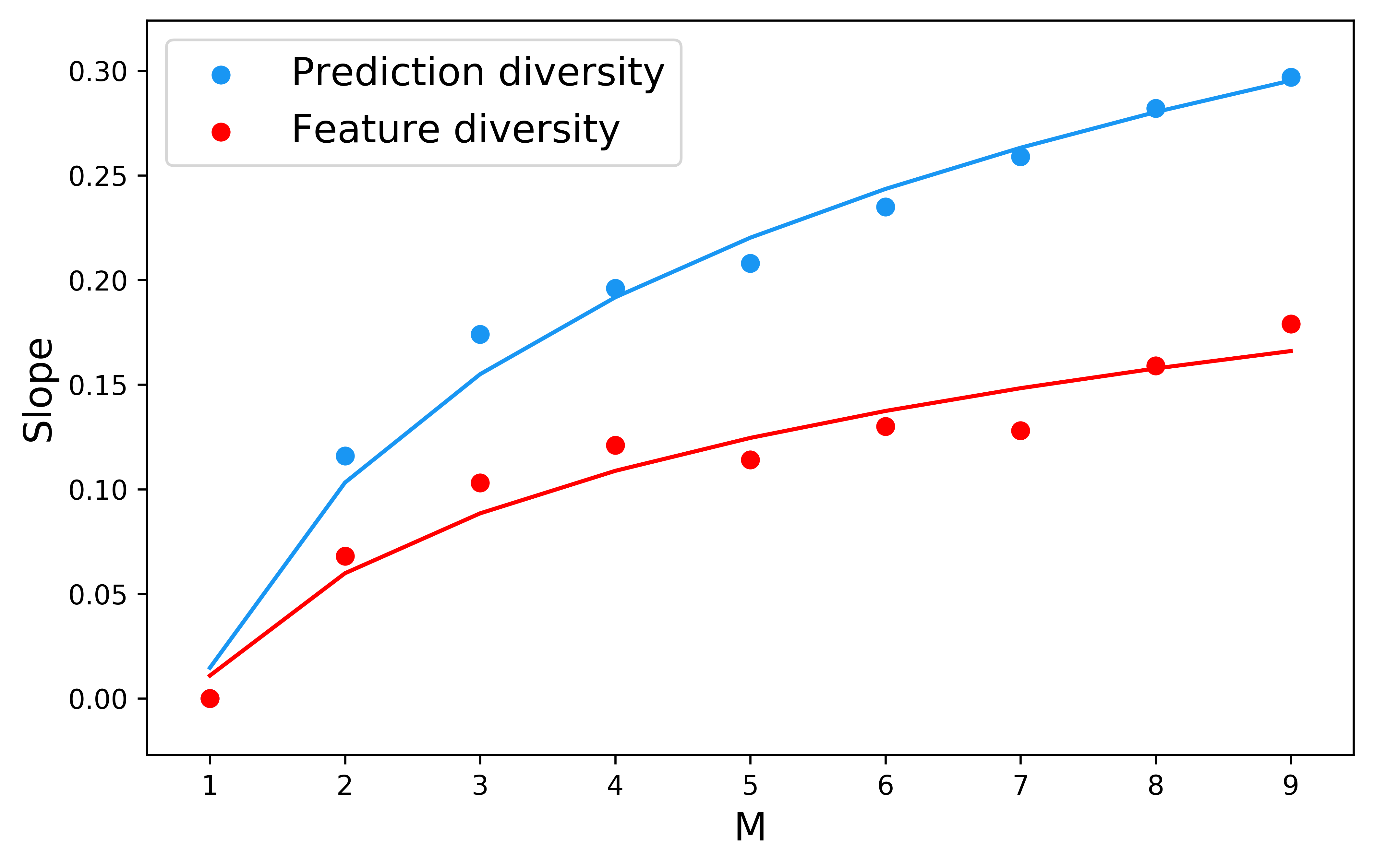
In Figures 2 and 10(a), we indicated the slope of the linear regressions relating diversity to accuracy gain at fixed $M$ (between $2$ and $9$). For example, when $M=9$ weights are averaged, the accuracy gain increases by $0.297$ per unit of additional diversity in prediction [46] (see Figure 2) and by $0.179$ per unit of additional diversity in features [47] (see Figure 10(a)). Most importantly, we note that the slope increases with $M$. To make this more visible, we plot slopes w.r.t. $M$ in Figure 11. Our observations are consistent with the $(M-1)/M$ factor in front of $\mathrm{cov}\mathopen{}\mathclose{{}\left(x}\right)$ in Equation BVCL. This shows that diversity becomes more important for large $M$. Yet, large $M$ is computationally impractical in standard functional ensembling, as one forward step is required per model. In contrast, WA has a fixed inference time which allows it to consider larger $M$. Increasing $M$ from $20$ to $60$ is the main reason why DiWA^† improves DiWA.

Figure 11: The slopes of linear regression — relating diversity to accuracy gain in Figure 2 and Figure 10(a) — increases with $M$.

E.1.3 Diversity comparison across a wide range of methods

Inspired by [21], we further analyze in Figure 12 the diversity between two weights obtained from different (more or less correlated) learning procedures.

• In the upper part, weights are obtained from a single run. They share the same initialization/hyperparameters/data/noise in the optimization procedure and only differ by the number of training steps (which we choose to be a multiple of $50$). They are less diverse than the weights in the middle part of Figure 12, that are sampled from two ERM runs.

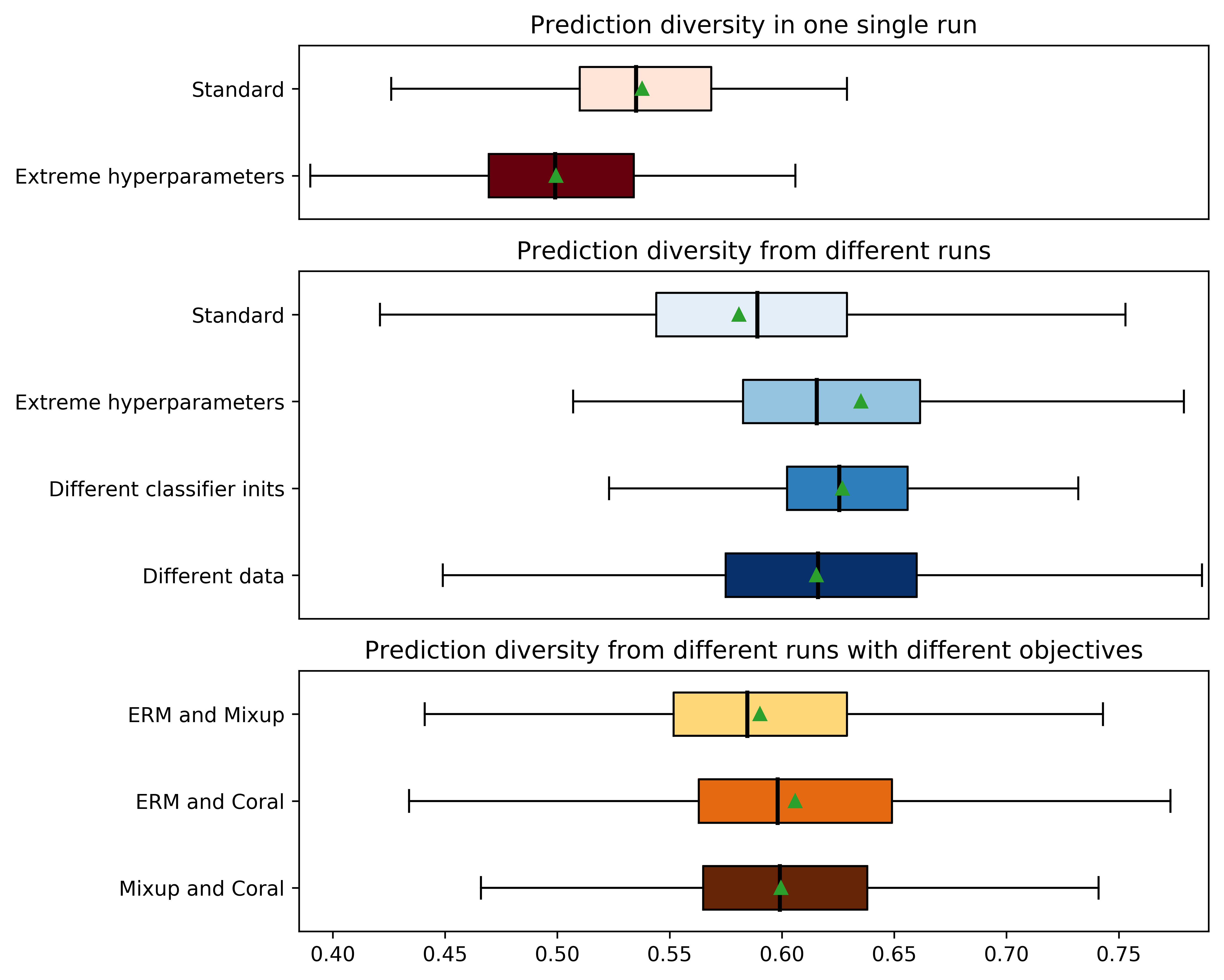
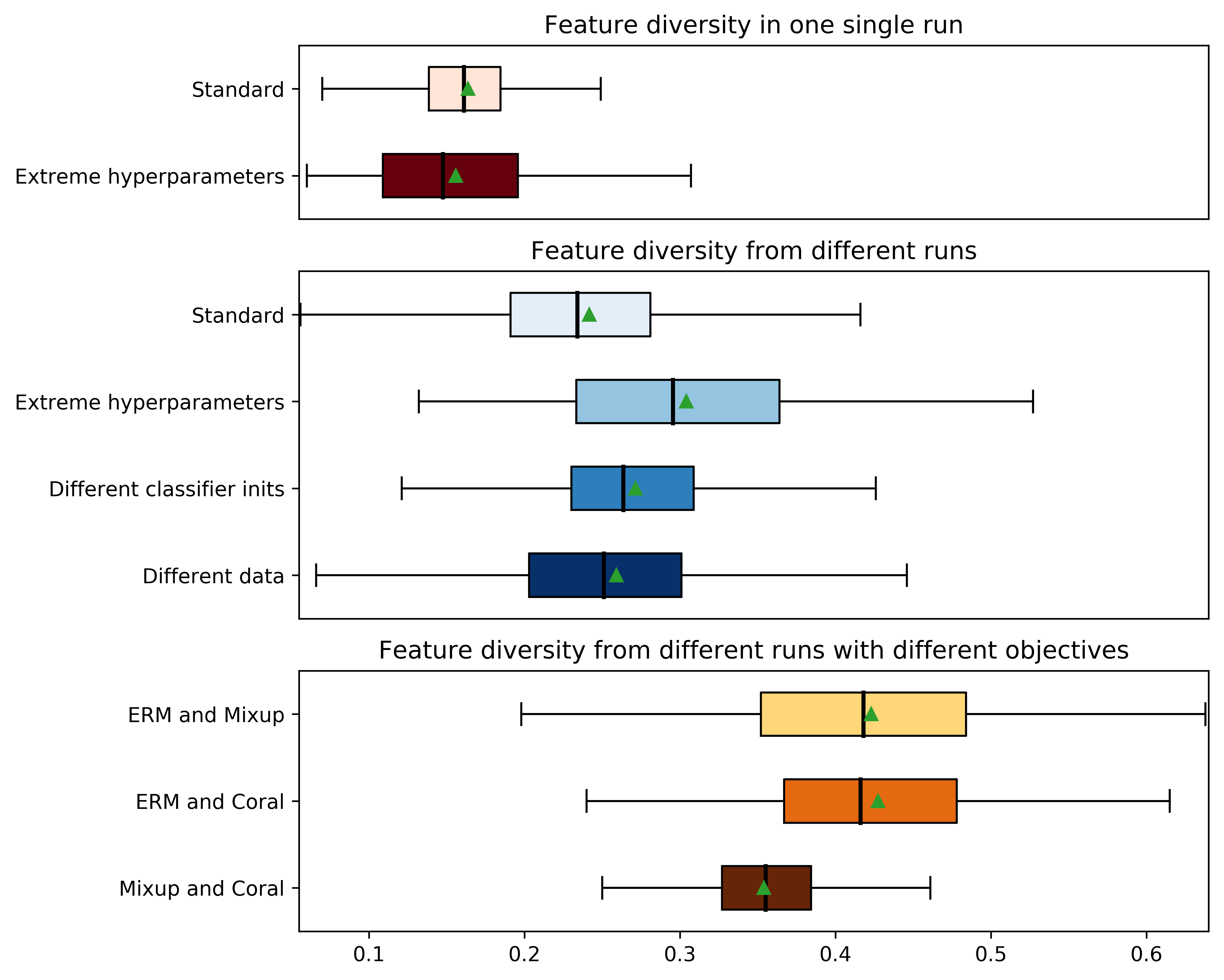
• When sampled from different runs, the weights become even more diverse when they have more extreme hyperparameter ranges, they do not share the same classifier initialization or they are trained on different data. The first two are impractical for WA, as it breaks the locality requirement (see Figures 5 and 10(c)). Luckily, the third setting “data diversity” is more convenient and is another reason for the success of DiWA^†; its $60$ weights were trained on $3$ different data splits. Data diversity has provable benefits [100], e.g., in bagging [68].

• Finally, we observe that diversity is increased (notably in features) when two runs have different objectives, for example, Interdomain Mixup [56] and Coral [10]. Thus incorporating weights trained with different invariance-based objectives have two benefits that explain the strong results in Table 2: (1) they learn invariant features by leveraging the domain information and (2) they enrich the diversity of solutions by extracting different features. These solutions can bring their own particularity to WA.

In conclusion, our analysis confirms that “model pairs that diverge more in training methodology display categorically different generalization behavior, producing increasingly uncorrelated errors”, as stated in [21].

(a) Prediction diversity [46].

(b) Feature diversity [47].

Figure 12: Diversity analysis across weights, which are per default trained with ERM, with a mild hyperparameter range (see Table 7), with a shared random classifier initialization, on a given data split. First, it confirms Figures 3 and 10(b): weights obtained from two different runs are more different than those sampled from a single run (even with extreme hyperparameters). Second, this shows that weights from two runs are more diverse when the two runs have different hyperparameters/data/classifier initializations/training objectives. Domain “Art” on OfficeHome.

E.1.4 Trade-off between diversity and averageability

We argue in Section 2.4.4 that our weights should ideally be diverse functionally while being averageable (despite the nonlinearities in the network). We know from [25] that models fine-tuned from a shared initialization with shared hyperparameters can be connected along a linear path where error remains low; thus, they are averageable as their WA also has a low loss. In Figure 5, we confirmed that averaging models from different initializations performs poorly. Regarding the hyperparameters, Figure 5 shows that hyperparameters can be selected slightly different but not too distant. That is why we chose mild hyperparameter ranges (defined in Table 7) in our main experiments.

A complete analysis of when the averageability holds when varying the different hyperparameters is a promising lead for future work. Still, Figure 13 is a preliminary investigation of the impact of different learning rates (between learning procedures of each weight). First, we validate that more distant learning rates lead to more functional diversity in Figure 13(a). Yet, we observe in Figure 13(b) that if learning rates are too different, weight averaging no longer approximates functional ensembling because the $O(\Delta_{L_{S}^{M}}^{2})$ term in Lemma 1 can be large.

(a) Prediction diversity ($\uparrow$) [46] between models.

(b) Accuracy ($\uparrow$) difference between DiWA and ENS.

Figure 13: Trade-off between diversity and averageability for various differences in learning rates. Considering $M=2$ weights obtained from two learning procedures with learning rates $\text{lr}_{1}$ and $\text{lr}_{2}$ (sampled from the extreme distribution in Table 7), we plot in Figure 13(a) the prediction diversity for these $M=2$ models vs. $|\text{lr}_{1}-\text{lr}_{2}|$. Then, in Figure 13(b), we plot the accuracy differences $\operatorname{Acc}(\text{DiWA})-\operatorname{Acc}(\text{ENS})$ vs. $|\text{lr}_{1}-\text{lr}_{2}|$.

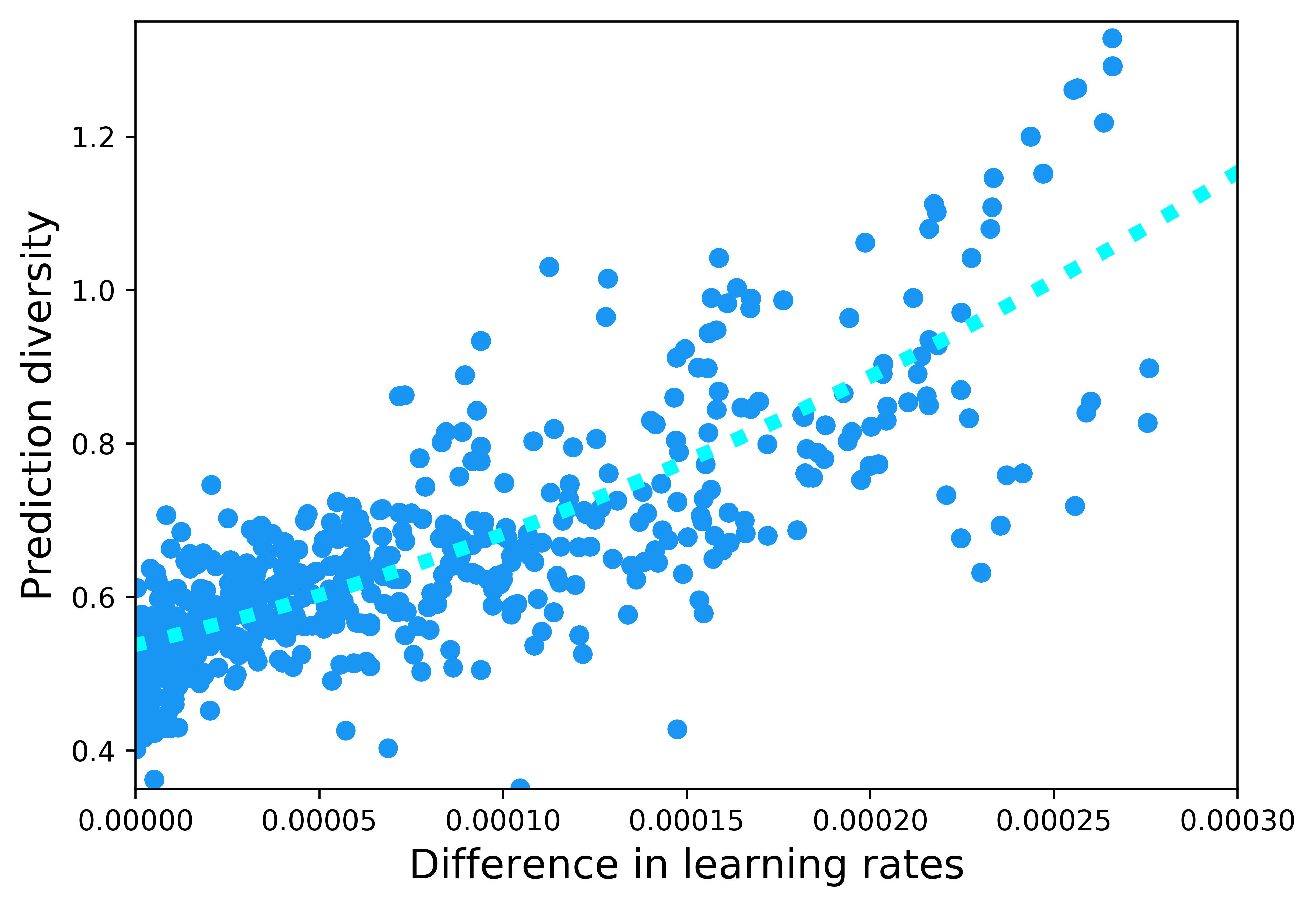
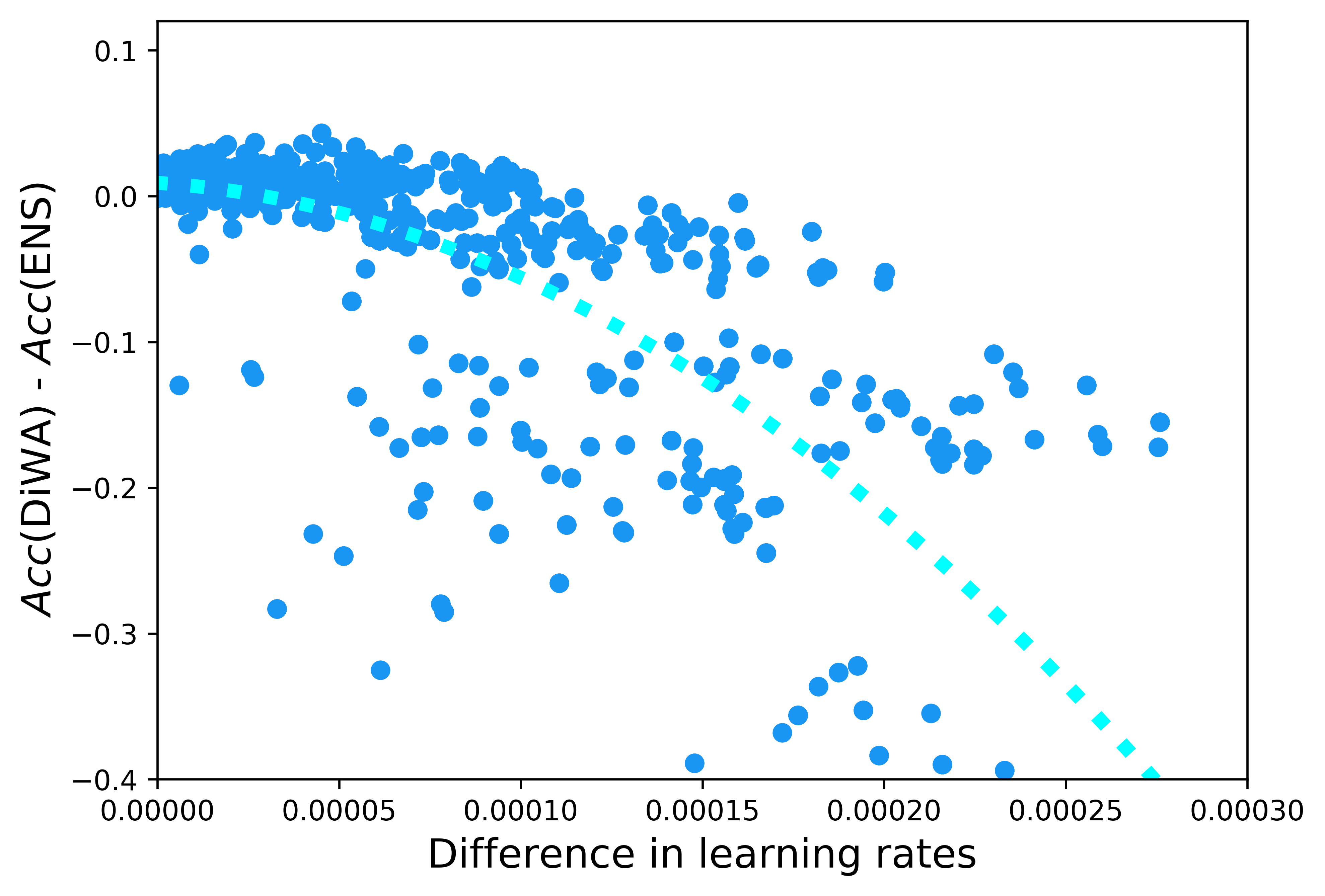
E.2 On PACS

We perform in Figure 14 on domain “Art” from PACS the same core diversity-based experiments than on OfficeHome in Section 4. We recover the same conclusions.

(a) Same as Figure 2.

(b) Same as Figure 10(a).

(c) Same as Figure 11.

Figure 14: Same analysis on PACS as previously done on OfficeHome.

(a) Same as Figure 3.

(b) Same as Figure 10(b).

(c) Same as Figure 4.

Figure 15: Same analysis on PACS as previously done on OfficeHome.

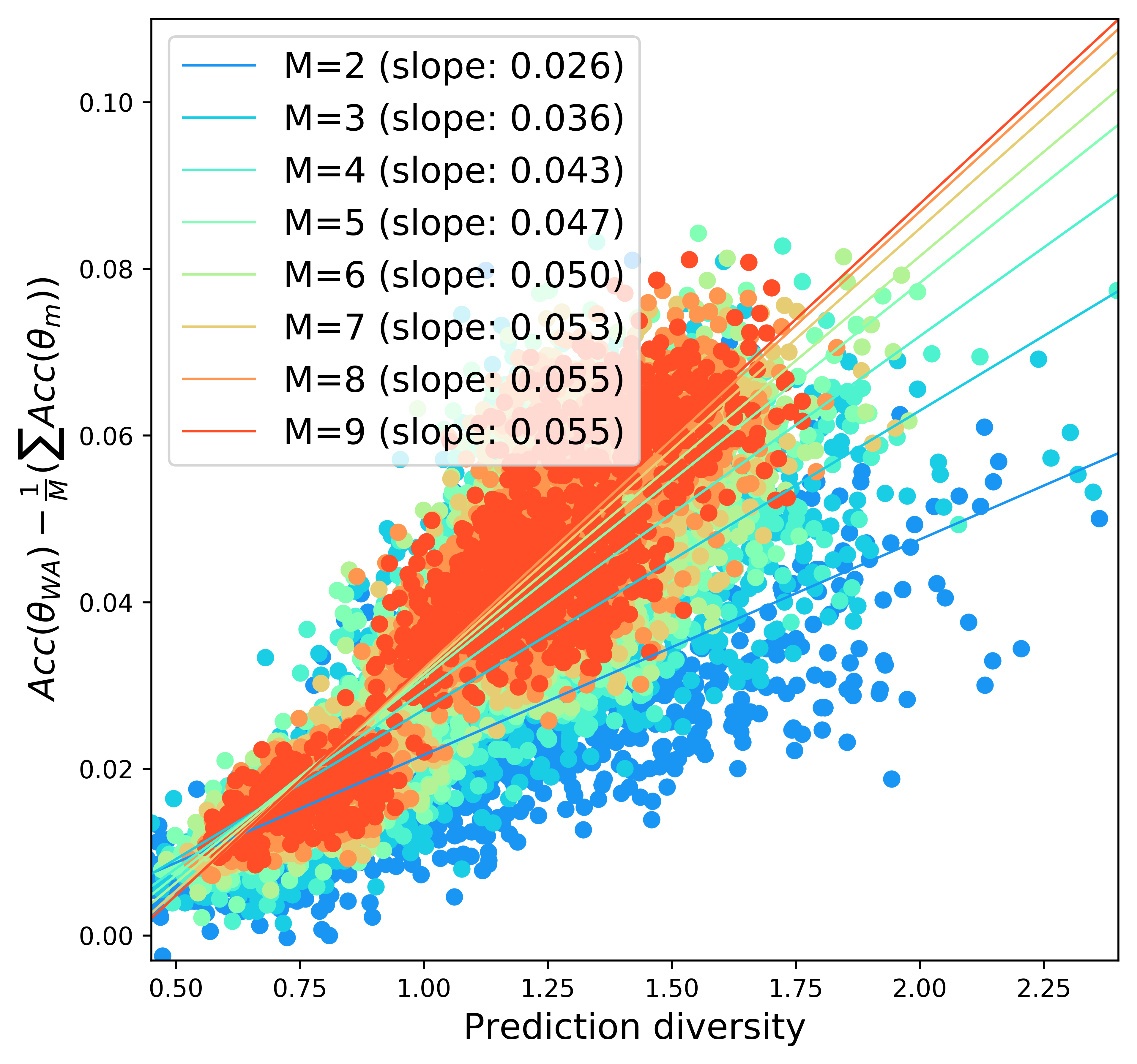
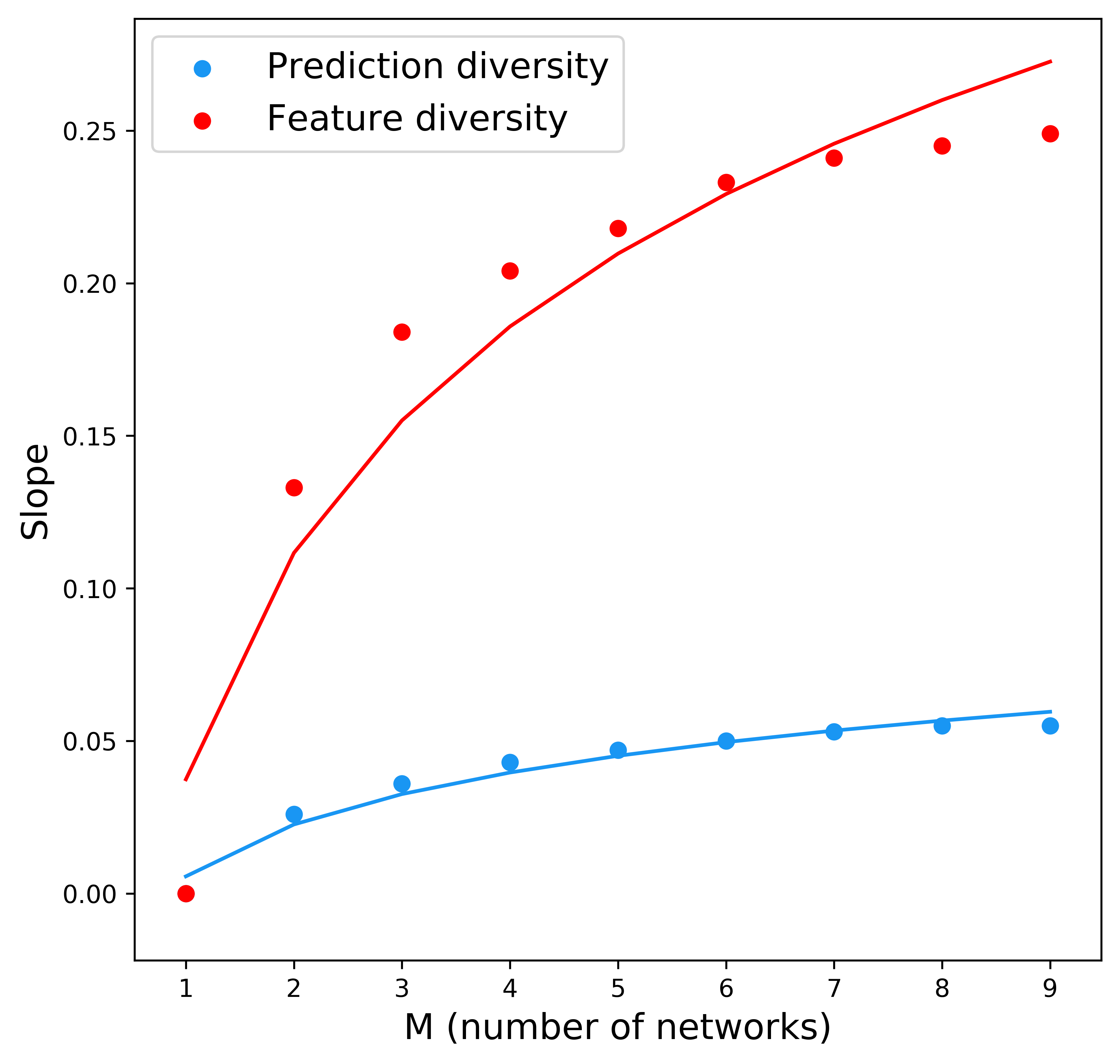
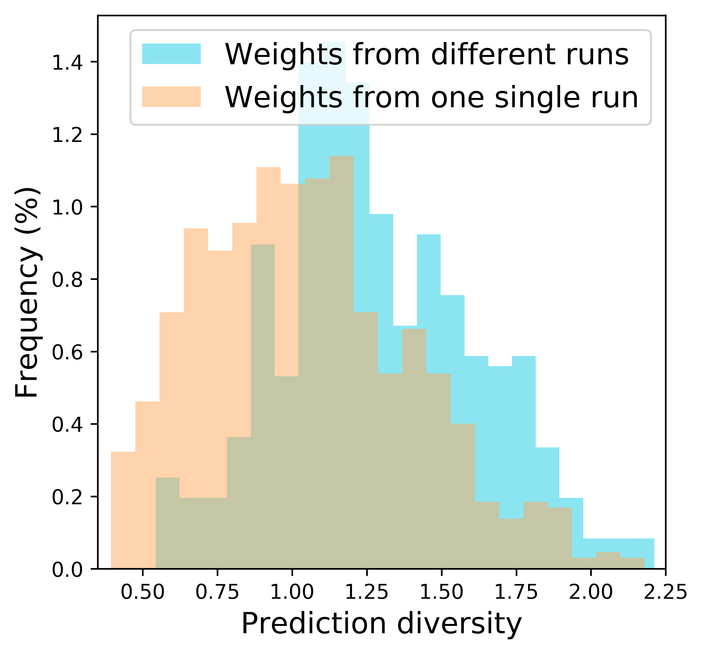
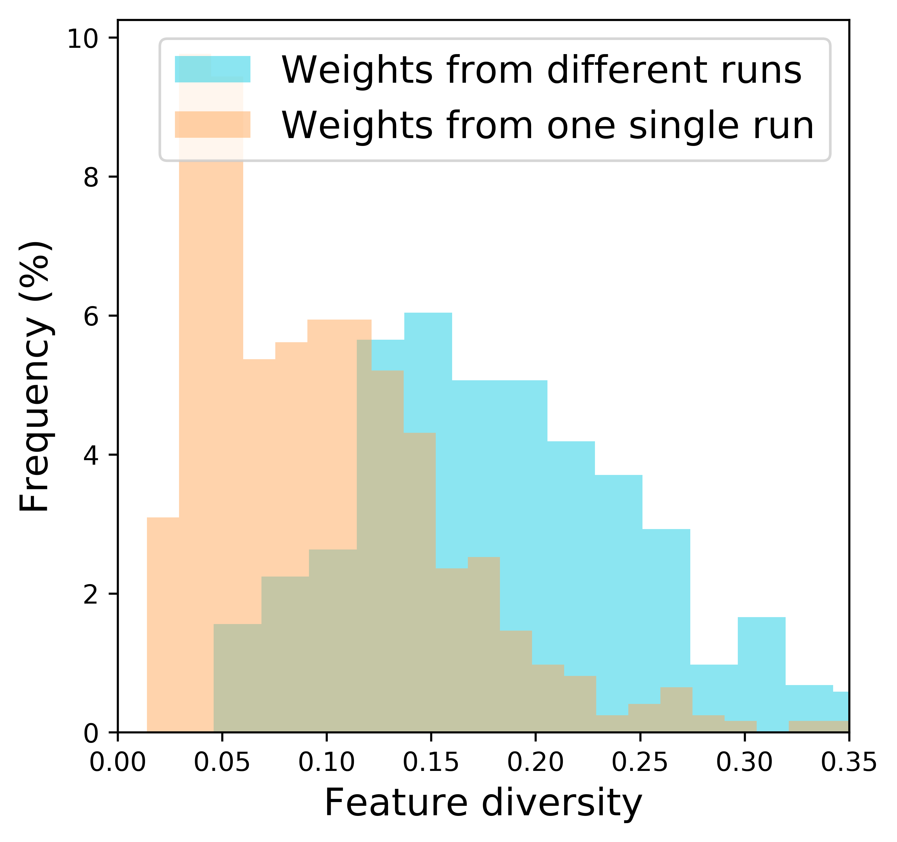
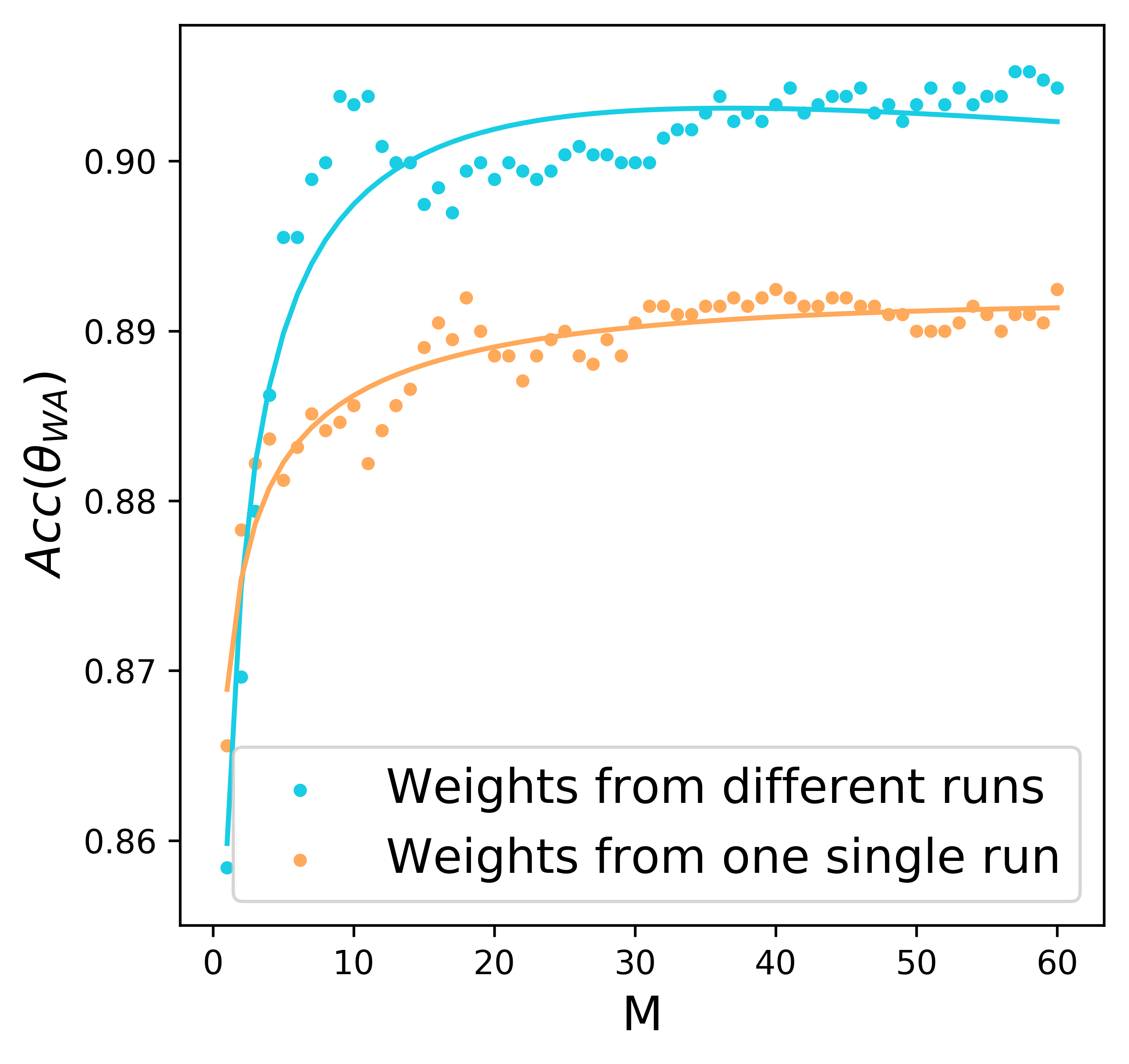
Appendix F Number of training runs

In our experiments, we train $20$ independent training runs per data split. We selected this value as $20$ is the standard number of hyperparameter trials in DomainBed [12]. In Figure 16 we ablate this choice on the OOD domain “Art” of OfficeHome. We observe that a larger number of runs leads to improved performance and reduced standard deviation. These results are consistent with our theoretical analysis, as the variance is divided per $M$ in Proposition 1. If reducing the training time is critical, one could benefit from significant gains over ERM even with a smaller number of runs: for example, $10$ runs seem sufficient in this case. This analysis complements Figure 4 — where $60$ runs were launched then sorted in increasing validation accuracy.

Figure 16: Mean and standard deviation of DiWA-uniform’s accuracy ($\uparrow$) on OfficeHome when increasing the number of training runs and uniformly averaging all weights. OOD accuracy is computed on domain “Art”, while IID accuracy is computed on validation data from the “Clipart”+“Product”+“Photo” domains.

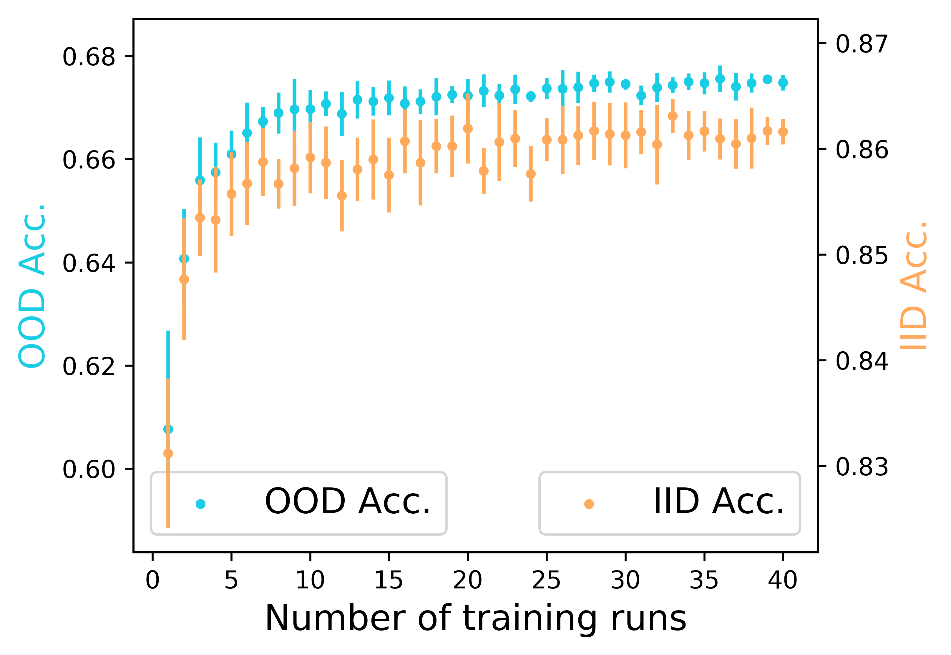
Moreover, in Table 6 we report DiWA’s results when considering only $5$ runs, with uniform weight selection. Interestingly, it shows that $M=5$ is enough to be competitive against SWAD [14], the previous state of the art.

Table 6: Accuracy ($\%,\uparrow$) on DomainBed. DiWA-uniform and LP initialization [49].

Algorithm PACS VLCS OfficeHome TerraInc DomainNet Avg SWAD [14] 88.1 $\pm$ 0.1 79.1 $\pm$ 0.1 70.6 $\pm$ 0.2 50.0 $\pm$ 0.3 46.5 $\pm$ 0.1 66.9 DiWA: $M=5$ 87.9 $\pm$ 0.2 78.3 $\pm$ 0.3 71.5 $\pm$ 0.2 51.0 $\pm$ 0.7 46.9 $\pm$ 0.3 67.1 DiWA: $M=20$ 88.7 $\pm$ 0.2 78.4 $\pm$ 0.2 72.1 $\pm$ 0.2 51.4 $\pm$ 0.6 47.4 $\pm$ 0.2 67.6 DiWA^†: $M=60$ 89.0 78.6 72.8 51.9 47.7 68.0

Appendix G DomainBed

G.1 Description of the DomainBed benchmark

We now further detail our experiments on the DomainBed benchmark [12].

Data.

DomainBed includes several computer vision classification datasets divided into multiple domains. Each domain is successively considered as the test domain while other domains are used in training. In practice, the data from each domain is split into 80% (used as training and testing) and 20% (used as validation for hyperparameter selection) splits. This random process is repeated with 3 different seeds: the reported numbers are the means and the standard errors over these 3 seeds.

Training protocol.

We follow the training protocol from https://github.com/facebookresearch/DomainBed. For each dataset, domain and seed, we perform a random search of $20$ trials on the hyperparameter distributions described in Table 7. Our mild distribution is taken directly from [14], yet could be adapted by dataset for better results. Even though these distributions are more restricted than the extreme distributions introduced [12], our ERM runs perform better. It leads to a total amount of $2640$ runs only for Table 1. In Appendix B, the $\rho$ hyperparameter for SAM is sampled from $[0.001,0.002,0.005,0.01,0.02,0.05]$. In Table 2, hyperparameters specific to Interdomain Mixup [56] (“mixup_alpha”) and Coral [10] (“mmd_gamma”) are sampled from the distributions defined in [12]. We use a ResNet50 [52] pretrained on ImageNet, with a dropout layer before the newly added dense layer and fine-tuned with frozen batch normalization layers. The optimizer is Adam [101]. Our classifier is either initialized randomly or with Linear Probing [49]; in the latter case, we first learn only the classifier (with the encoder frozen) with the default hyperparameters defined in Table 7; the classifier’s weights are then used to initialize all subsequent runs. All runs are trained for 5k steps, except on DomainNet with 15k steps as done in concurrent works [14, 29]. As in [14], validation accuracy is calculated every $50$ steps for VLCS, $500$ steps for DomainNet and $100$ steps for others.

Table 7: Hyperparameters, their default values and distributions for random search.

Hyperparameter	Default value	Random distribution
		Extreme	Mild
		(DomainBed [12])	(DiWA as [14])
Learning rate	$5\cdot 10^{-5}$	$10^{\mathcal{U}(-5,-3.5)}$	$[1,3,5]\cdot 10^{-5}$
Batch size	$32$	$2^{\mathcal{U}(3,5.5)}$	$32$
ResNet dropout	$0$	$[0,0.1,0.5]$	$[0,0.1,0.5]$
Weight decay	$0$	$10^{\mathcal{U}(-6,-2)}$	$[10^{-6},10^{-4}]$

Model selection and scores.

We consider the training-domain validation set protocol. From each run, we thus take the weights of the epoch with maximum accuracy on the validation dataset — which follows the training distribution. Our restricted weight selection is also based on this training-domain validation set. This strategy is not possible for DiWA^† as it averages $M=20\times 3$ weights trained with different data splits: they do not share a common validation dataset. The scores for ERM and Coral are taken from DomainBed [12]. Scores for SWAD [14] and MA [29] are taken from their respective papers. Note that MA and SWAD perform similarly even though SWAD introduced three additional hyperparameters tuned per dataset: “an optimum patient parameter, an overfitting patient parameter, and the tolerance rate for searching the start iteration and the end iteration”. Thus we reproduced MA [29] which was much easier to implement, and closer to our uniform weight selection.

G.2 DomainBed results detailed per domain for each real-world dataset

Tables below detail results per domain for the $5$ multi-domain real-world datasets from DomainBed: PACS [51], VLCS [53], OfficeHome [50], TerraIncognita [54] and DomainNet [55]. Critically, [19] showed that diversity shift dominates in these datasets.

Table 8: Accuracy ($\%,\uparrow$) on PACS with ResNet50 (best in bold and second best underlined).

Algorithm Weight selection Init A C P S Avg ERM N/A Random 84.7 $\pm$ 0.4 80.8 $\pm$ 0.6 97.2 $\pm$ 0.3 79.3 $\pm$ 1.0 85.5 $\pm$ 0.2 Coral[10] N/A 88.3 $\pm$ 0.2 80.0 $\pm$ 0.5 97.5 $\pm$ 0.3 78.8 $\pm$ 1.3 86.2 $\pm$ 0.3 SWAD [14] Overfit-aware 89.3 $\pm$ 0.5 83.4 $\pm$ 0.6 97.3 $\pm$ 0.3 82.5 $\pm$ 0.8 88.1 $\pm$ 0.1 MA [29] Uniform 89.1 $\pm$ 0.1 82.6 $\pm$ 0.2 97.6 $\pm$ 0.0 80.5 $\pm$ 0.9 87.5 $\pm$ 0.2 DENS [15, 29] Uniform: $M=6$ 88.3 83.6 96.5 81.9 87.6 Our runs ERM N/A Random 87.6 $\pm$ 0.4 80.1 $\pm$ 1.5 97.7 $\pm$ 0.3 76.7 $\pm$ 1.2 85.5 $\pm$ 0.5 MA [29] Uniform 89.9 $\pm$ 0.1 83.3 $\pm$ 0.4 97.8 $\pm$ 0.2 80.6 $\pm$ 0.3 87.9 $\pm$ 0.1 ENS Uniform: $M=20$ 88.9 $\pm$ 0.4 82.3 $\pm$ 0.5 97.4 $\pm$ 0.3 83.2 $\pm$ 0.3 88.0 $\pm$ 0.1 DiWA Restricted: $M\leq 20$ 90.0 $\pm$ 0.3 82.0 $\pm$ 0.5 97.5 $\pm$ 0.1 82.0 $\pm$ 0.6 87.9 $\pm$ 0.2 DiWA Uniform: $M=20$ 90.1 $\pm$ 0.6 83.3 $\pm$ 0.6 98.2 $\pm$ 0.1 83.4 $\pm$ 0.4 88.8 $\pm$ 0.4 DiWA^† Uniform: $M=60$ 90.5 83.7 98.2 83.8 89.0 ERM N/A LP [49] 86.8 $\pm$ 0.8 80.6 $\pm$ 1.0 97.4 $\pm$ 0.4 78.7 $\pm$ 2.0 85.9 $\pm$ 0.6 MA [29] Uniform 89.5 $\pm$ 0.1 82.8 $\pm$ 0.2 97.8 $\pm$ 0.1 80.9 $\pm$ 1.3 87.8 $\pm$ 0.3 ENS Uniform: $M=20$ 89.6 $\pm$ 0.2 81.6 $\pm$ 0.3 97.8 $\pm$ 0.2 83.5 $\pm$ 0.5 88.1 $\pm$ 0.3 DiWA Restricted: $M\leq 20$ 89.3 $\pm$ 0.2 82.8 $\pm$ 0.2 98.0 $\pm$ 0.1 82.0 $\pm$ 0.9 88.0 $\pm$ 0.3 DiWA Uniform: $M=5$ 89.9 $\pm$ 0.5 82.3 $\pm$ 0.3 97.7 $\pm$ 0.4 81.7 $\pm$ 0.8 87.9 $\pm$ 0.2 DiWA Uniform: $M=20$ 90.1 $\pm$ 0.2 82.8 $\pm$ 0.6 98.3 $\pm$ 0.1 83.3 $\pm$ 0.4 88.7 $\pm$ 0.2 DiWA^† Uniform: $M=60$ 90.6 83.4 98.2 83.8 89.0

Table 9: Accuracy ($\%,\uparrow$) on VLCS with ResNet50 (best in bold and second best underlined).

Algorithm Weight selection Init C L S V Avg ERM N/A Random 97.7 $\pm$ 0.4 64.3 $\pm$ 0.9 73.4 $\pm$ 0.5 74.6 $\pm$ 1.3 77.5 $\pm$ 0.4 Coral[10] N/A 98.3 $\pm$ 0.1 66.1 $\pm$ 1.2 73.4 $\pm$ 0.3 77.5 $\pm$ 1.2 78.8 $\pm$ 0.6 SWAD [14] Overfit-aware 98.8 $\pm$ 0.1 63.3 $\pm$ 0.3 75.3 $\pm$ 0.5 79.2 $\pm$ 0.6 79.1 $\pm$ 0.1 MA [29] Uniform 99.0 $\pm$ 0.2 63.0 $\pm$ 0.2 74.5 $\pm$ 0.3 76.4 $\pm$ 1.1 78.2 $\pm$ 0.2 DENS [15, 29] Uniform: $M=6$ 98.7 64.5 72.1 78.9 78.5 Our runs ERM N/A Random 97.9 $\pm$ 0.5 64.2 $\pm$ 0.3 73.5 $\pm$ 0.5 74.9 $\pm$ 1.2 77.6 $\pm$ 0.2 MA [29] Uniform 98.5 $\pm$ 0.2 63.5 $\pm$ 0.2 74.4 $\pm$ 0.8 77.3 $\pm$ 0.3 78.4 $\pm$ 0.1 ENS Uniform: $M=20$ 98.6 $\pm$ 0.1 64.9 $\pm$ 0.2 73.5 $\pm$ 0.3 77.7 $\pm$ 0.3 78.7 $\pm$ 0.1 DiWA Restricted: $M\leq 20$ 98.3 $\pm$ 0.1 63.9 $\pm$ 0.2 75.6 $\pm$ 0.2 79.1 $\pm$ 0.3 79.2 $\pm$ 0.1 DiWA Uniform: $M=20$ 98.4 $\pm$ 0.1 63.4 $\pm$ 0.1 75.5 $\pm$ 0.3 78.9 $\pm$ 0.6 79.1 $\pm$ 0.2 DiWA^† Uniform: $M=60$ 98.4 63.3 76.1 79.6 79.4 ERM N/A LP [49] 98.1 $\pm$ 0.3 64.4 $\pm$ 0.3 72.5 $\pm$ 0.5 77.7 $\pm$ 1.3 78.1 $\pm$ 0.5 MA [29] Uniform 98.9 $\pm$ 0.0 62.9 $\pm$ 0.5 73.7 $\pm$ 0.3 78.7 $\pm$ 0.6 78.5 $\pm$ 0.4 ENS Uniform: $M=20$ 98.5 $\pm$ 0.1 64.9 $\pm$ 0.1 73.4 $\pm$ 0.4 77.2 $\pm$ 0.4 78.5 $\pm$ 0.1 DiWA Restricted: $M\leq 20$ 98.4 $\pm$ 0.0 64.1 $\pm$ 0.2 73.3 $\pm$ 0.4 78.1 $\pm$ 0.8 78.5 $\pm$ 0.1 DiWA Uniform: $M=5$ 98.8 $\pm$ 0.0 63.8 $\pm$ 0.5 72.9 $\pm$ 0.2 77.6 $\pm$ 0.5 78.3 $\pm$ 0.3 DiWA Uniform: $M=20$ 98.8 $\pm$ 0.1 62.8 $\pm$ 0.2 73.9 $\pm$ 0.3 78.3 $\pm$ 0.1 78.4 $\pm$ 0.2 DiWA^† Uniform: $M=60$ 98.9 62.4 73.9 78.9 78.6

Table 10: Accuracy ($\%,\uparrow$) on OfficeHome with ResNet50 (best in bold and second best underlined).

Algorithm Weight selection Init A C P R Avg ERM N/A Random 61.3 $\pm$ 0.7 52.4 $\pm$ 0.3 75.8 $\pm$ 0.1 76.6 $\pm$ 0.3 66.5 $\pm$ 0.3 Coral[10] N/A 65.3 $\pm$ 0.4 54.4 $\pm$ 0.5 76.5 $\pm$ 0.1 78.4 $\pm$ 0.5 68.7 $\pm$ 0.3 SWAD [14] Overfit-aware 66.1 $\pm$ 0.4 57.7 $\pm$ 0.4 78.4 $\pm$ 0.1 80.2 $\pm$ 0.2 70.6 $\pm$ 0.2 MA [29] Uniform 66.7 $\pm$ 0.5 57.1 $\pm$ 0.1 78.6 $\pm$ 0.1 80.0 $\pm$ 0.0 70.6 $\pm$ 0.1 DENS [15, 29] Uniform: $M=6$ 65.6 58.5 78.7 80.5 70.8 Our runs ERM N/A Random 62.9 $\pm$ 1.3 54.0 $\pm$ 0.2 75.7 $\pm$ 0.9 77.0 $\pm$ 0.8 67.4 $\pm$ 0.6 MA [29] Uniform 65.0 $\pm$ 0.2 57.9 $\pm$ 0.3 78.5 $\pm$ 0.1 79.7 $\pm$ 0.1 70.3 $\pm$ 0.1 ENS Uniform: $M=20$ 66.1 $\pm$ 0.1 57.0 $\pm$ 0.3 79.0 $\pm$ 0.2 80.0 $\pm$ 0.1 70.5 $\pm$ 0.1 DiWA Restricted: $M\leq 20$ 66.7 $\pm$ 0.1 57.0 $\pm$ 0.3 78.5 $\pm$ 0.3 79.9 $\pm$ 0.3 70.5 $\pm$ 0.1 DiWA Uniform: $M=20$ 67.3 $\pm$ 0.2 57.9 $\pm$ 0.2 79.0 $\pm$ 0.2 79.9 $\pm$ 0.1 71.0 $\pm$ 0.1 DiWA^† Uniform: $M=60$ 67.7 58.8 79.4 80.5 71.6 ERM N/A LP [49] 63.9 $\pm$ 1.2 54.8 $\pm$ 0.6 78.7 $\pm$ 0.1 80.4 $\pm$ 0.2 69.4 $\pm$ 0.2 MA [29] Uniform 67.4 $\pm$ 0.4 57.3 $\pm$ 0.9 79.7 $\pm$ 0.1 81.7 $\pm$ 0.6 71.5 $\pm$ 0.3 ENS Uniform: $M=20$ 67.0 $\pm$ 0.1 57.9 $\pm$ 0.4 80.0 $\pm$ 0.2 81.7 $\pm$ 0.3 71.7 $\pm$ 0.1 DiWA Restricted: $M\leq 20$ 67.8 $\pm$ 0.5 57.2 $\pm$ 0.5 79.6 $\pm$ 0.1 81.4 $\pm$ 0.4 71.5 $\pm$ 0.2 DiWA Uniform: $M=5$ 68.4 $\pm$ 0.4 57.4 $\pm$ 0.5 79.2 $\pm$ 0.2 80.9 $\pm$ 0.4 71.5 $\pm$ 0.3 DiWA Uniform: $M=20$ 68.4 $\pm$ 0.2 58.2 $\pm$ 0.5 80.0 $\pm$ 0.1 81.7 $\pm$ 0.3 72.1 $\pm$ 0.2 DiWA^† Uniform: $M=60$ 69.2 59.0 80.6 82.2 72.8

Table 11: Accuracy ($\%,\uparrow$) on TerraIncognita with ResNet50 (best in bold and second best underlined).

Algorithm Weight selection Init L100 L38 L43 L46 Avg ERM N/A Random 49.8 $\pm$ 4.4 42.1 $\pm$ 1.4 56.9 $\pm$ 1.8 35.7 $\pm$ 3.9 46.1 $\pm$ 1.8 Coral[10] N/A 51.6 $\pm$ 2.4 42.2 $\pm$ 1.0 57.0 $\pm$ 1.0 39.8 $\pm$ 2.9 47.6 $\pm$ 1.0 SWAD [14] Overfit-aware 55.4 $\pm$ 0.0 44.9 $\pm$ 1.1 59.7 $\pm$ 0.4 39.9 $\pm$ 0.2 50.0 $\pm$ 0.3 MA [29] Uniform 54.9 $\pm$ 0.4 45.5 $\pm$ 0.6 60.1 $\pm$ 1.5 40.5 $\pm$ 0.4 50.3 $\pm$ 0.5 DENS [15, 29] Uniform: $M=6$ 53.0 42.6 60.5 40.8 49.2 Our runs ERM N/A Random 56.3 $\pm$ 2.9 43.1 $\pm$ 1.6 57.1 $\pm$ 1.0 36.7 $\pm$ 0.7 48.3 $\pm$ 0.8 MA [29] Uniform 53.2 $\pm$ 0.4 46.3 $\pm$ 1.0 60.1 $\pm$ 0.6 40.2 $\pm$ 0.8 49.9 $\pm$ 0.2 ENS Uniform: $M=20$ 56.4 $\pm$ 1.5 45.3 $\pm$ 0.4 61.0 $\pm$ 0.3 41.4 $\pm$ 0.5 51.0 $\pm$ 0.5 DiWA Restricted: $M\leq 20$ 55.6 $\pm$ 1.5 47.5 $\pm$ 0.5 59.5 $\pm$ 0.5 39.4 $\pm$ 0.2 50.5 $\pm$ 0.5 DiWA Uniform: $M=20$ 52.2 $\pm$ 1.8 46.2 $\pm$ 0.4 59.2 $\pm$ 0.2 37.8 $\pm$ 0.6 48.9 $\pm$ 0.5 DiWA^† Uniform: $M=60$ 52.7 46.3 59.0 37.7 49.0 ERM N/A LP [49] 59.9 $\pm$ 4.2 46.9 $\pm$ 0.9 54.6 $\pm$ 0.3 40.1 $\pm$ 2.2 50.4 $\pm$ 1.8 MA [29] Uniform 54.6 $\pm$ 1.4 48.6 $\pm$ 0.4 59.9 $\pm$ 0.7 42.7 $\pm$ 0.8 51.4 $\pm$ 0.6 ENS Uniform: $M=20$ 55.6 $\pm$ 1.4 45.4 $\pm$ 0.4 61.0 $\pm$ 0.4 41.3 $\pm$ 0.3 50.8 $\pm$ 0.5 DiWA Restricted: $M\leq 20$ 58.5 $\pm$ 2.2 48.2 $\pm$ 0.3 58.5 $\pm$ 0.3 41.1 $\pm$ 1.2 51.6 $\pm$ 0.9 DiWA Uniform: $M=5$ 56.0 $\pm$ 2.5 48.9 $\pm$ 0.8 58.4 $\pm$ 0.2 40.6 $\pm$ 0.8 51.0 $\pm$ 0.7 DiWA Uniform: $M=20$ 56.3 $\pm$ 1.9 49.4 $\pm$ 0.7 59.9 $\pm$ 0.4 39.8 $\pm$ 0.5 51.4 $\pm$ 0.6 DiWA^† Uniform: $M=60$ 57.2 50.1 60.3 39.8 51.9

Table 12: Accuracy ($\%,\uparrow$) on DomainNet with ResNet50 (best in bold and second best underlined).

Algorithm Weight selection Init clip info paint quick real sketch Avg ERM N/A Random 58.1 $\pm$ 0.3 18.8 $\pm$ 0.3 46.7 $\pm$ 0.3 12.2 $\pm$ 0.4 59.6 $\pm$ 0.1 49.8 $\pm$ 0.4 40.9 $\pm$ 0.1 Coral[10] N/A 59.2 $\pm$ 0.1 19.7 $\pm$ 0.2 46.6 $\pm$ 0.3 13.4 $\pm$ 0.4 59.8 $\pm$ 0.2 50.1 $\pm$ 0.6 41.5 $\pm$ 0.1 SWAD [14] Overfit-aware 66.0 $\pm$ 0.1 22.4 $\pm$ 0.3 53.5 $\pm$ 0.1 16.1 $\pm$ 0.2 65.8 $\pm$ 0.4 55.5 $\pm$ 0.3 46.5 $\pm$ 0.1 MA [29] Uniform 64.4 $\pm$ 0.3 22.4 $\pm$ 0.2 53.4 $\pm$ 0.3 15.4 $\pm$ 0.1 64.7 $\pm$ 0.2 55.5 $\pm$ 0.1 46.0 $\pm$ 0.1 DENS [15, 29] Uniform: $M=6$ 68.3 23.1 54.5 16.3 66.9 57.0 47.7 Our runs ERM N/A Random 62.6 $\pm$ 0.4 21.6 $\pm$ 0.3 50.4 $\pm$ 0.1 13.8 $\pm$ 0.2 63.6 $\pm$ 0.4 52.5 $\pm$ 0.4 44.1 $\pm$ 0.1 MA [29] Uniform 64.5 $\pm$ 0.2 22.7 $\pm$ 0.1 53.8 $\pm$ 0.1 15.6 $\pm$ 0.1 66.0 $\pm$ 0.1 55.7 $\pm$ 0.1 46.4 $\pm$ 0.1 ENS Uniform: $M=20$ 67.3 $\pm$ 0.4 22.9 $\pm$ 0.1 54.2 $\pm$ 0.2 15.5 $\pm$ 0.2 67.7 $\pm$ 0.2 56.7 $\pm$ 0.2 47.4 $\pm$ 0.2 DiWA Restricted: $M\leq 20$ 65.2 $\pm$ 0.3 23.0 $\pm$ 0.3 54.0 $\pm$ 0.1 15.9 $\pm$ 0.1 66.2 $\pm$ 0.1 55.5 $\pm$ 0.1 46.7 $\pm$ 0.1 DiWA Uniform: $M=20$ 63.4 $\pm$ 0.2 23.1 $\pm$ 0.1 53.9 $\pm$ 0.2 15.4 $\pm$ 0.2 65.5 $\pm$ 0.2 55.1 $\pm$ 0.2 46.1 $\pm$ 0.1 DiWA^† Uniform: $M=60$ 63.5 23.3 54.3 15.6 65.7 55.3 46.3 ERM N/A LP [49] 63.4 $\pm$ 0.2 21.1 $\pm$ 0.4 50.7 $\pm$ 0.3 13.5 $\pm$ 0.4 64.8 $\pm$ 0.4 52.4 $\pm$ 0.1 44.3 $\pm$ 0.2 MA [29] Uniform 64.8 $\pm$ 0.1 22.3 $\pm$ 0.0 54.2 $\pm$ 0.1 16.0 $\pm$ 0.1 67.4 $\pm$ 0.0 55.2 $\pm$ 0.1 46.6 $\pm$ 0.0 ENS Uniform: $M=20$ 66.7 $\pm$ 0.4 22.2 $\pm$ 0.1 54.1 $\pm$ 0.2 15.1 $\pm$ 0.2 68.4 $\pm$ 0.1 55.7 $\pm$ 0.2 47.0 $\pm$ 0.2 DiWA Restricted: $M\leq 20$ 66.7 $\pm$ 0.2 23.3 $\pm$ 0.2 55.3 $\pm$ 0.1 16.3 $\pm$ 0.2 68.2 $\pm$ 0.0 56.2 $\pm$ 0.1 47.7 $\pm$ 0.1 DiWA Uniform: $M=5$ 65.7 $\pm$ 0.5 22.6 $\pm$ 0.2 54.4 $\pm$ 0.4 15.5 $\pm$ 0.5 67.7 $\pm$ 0.0 55.5 $\pm$ 0.4 46.9 $\pm$ 0.3 DiWA Uniform: $M=20$ 65.9 $\pm$ 0.4 23.0 $\pm$ 0.2 55.0 $\pm$ 0.3 16.1 $\pm$ 0.2 68.4 $\pm$ 0.1 55.7 $\pm$ 0.4 47.4 $\pm$ 0.2 DiWA^† Uniform: $M=60$ 66.2 23.3 55.4 16.5 68.7 56.0 47.7

Appendix H Failure of WA under correlation shift on ColoredMNIST

Based on Equation BVCL, we explained that WA is efficient when variance dominates; we showed in Section 2.4.2 that this occurs under diversity shift. This is confirmed by our state-of-the-art results in Table 1 and Section G.2 on PACS, OfficeHome, VLCS, TerraIncognita and DomainNet. In contrast, we argue that WA is inefficient when bias dominates, i.e., in the presence of correlation shift (see Section 2.4.1). We verify this failure on the ColoredMNIST [8] dataset, which is dominated by correlation shift [55].

Colored MNIST is a colored variant of the MNIST handwritten digit classification dataset [102] where the correlation strengths between color and label vary across domains. We follow the protocol described in Section G.1 except that (1) we used the convolutional neural network architecture introduced in DomainBed [12] for MNIST experiments and (2) we used the test-domain model selection in addition to the train-domain model selection. Indeed, as stated in [19], “it may be improper to apply training-domain validation to datasets dominated by correlation shift since under the influence of spurious correlations, achieving excessively high accuracy in the training environments often leads to low accuracy in novel test environments”.

In Tables 13 and 14, we observe that DiWA-uniform and MA both perform poorly compared to ERM. Note that DiWA-restricted does not degrade ERM as it selects only a few models for averaging (low $M$). This confirms that our approach is useful to tackle diversity shift but not correlation shift, for which invariance-based approaches as IRM [8] or Fishr [11] remain state-of-the-art.

Table 13: Accuracy ($\%,\uparrow$) on ColoredMNIST. WA does not improve performance under correlation shift. Random initialization of the classifier. Training-domain model selection.

Algorithm Weight selection +90% +80% -90% Avg ERM N/A 71.7 $\pm$ 0.1 72.9 $\pm$ 0.2 10.0 $\pm$ 0.1 51.5 $\pm$ 0.1 Coral [10] N/A 71.6 $\pm$ 0.3 73.1 $\pm$ 0.1 9.9 $\pm$ 0.1 51.5 $\pm$ 0.1 IRM [8] N/A 72.5 $\pm$ 0.1 73.3 $\pm$ 0.5 10.2 $\pm$ 0.3 52.0 $\pm$ 0.1 Fishr [11] N/A 72.3 $\pm$ 0.9 73.5 $\pm$ 0.2 10.1 $\pm$ 0.2 52.0 $\pm$ 0.2 Our runs ERM N/A 71.5 $\pm$ 0.4 73.3 $\pm$ 0.2 10.3 $\pm$ 0.2 51.7 $\pm$ 0.2 MA [29] Uniform 68.9 $\pm$ 0.0 71.8 $\pm$ 0.1 10.0 $\pm$ 0.1 50.3 $\pm$ 0.0 ENS Uniform: $M=20$ 71.0 $\pm$ 0.2 72.9 $\pm$ 0.2 9.9 $\pm$ 0.0 51.3 $\pm$ 0.1 DiWA Restricted: $M\leq 20$ 71.3 $\pm$ 0.2 72.9 $\pm$ 0.1 10.0 $\pm$ 0.1 51.4 $\pm$ 0.1 DiWA Uniform: $M=20$ 69.1 $\pm$ 0.8 72.6 $\pm$ 0.4 10.6 $\pm$ 0.1 50.8 $\pm$ 0.4 DiWA^† Uniform: $M=60$ 69.3 72.3 10.3 50.6

Table 14: Accuracy ($\%,\uparrow$) on ColoredMNIST. WA does not improve performance under correlation shift. Random initialization of the classifier. Test-domain model selection.

Algorithm Weight selection +90% +80% -90% Avg ERM N/A 71.8 $\pm$ 0.4 72.9 $\pm$ 0.1 28.7 $\pm$ 0.5 57.8 $\pm$ 0.2 Coral [10] N/A 71.1 $\pm$ 0.2 73.4 $\pm$ 0.2 31.1 $\pm$ 1.6 58.6 $\pm$ 0.5 IRM [8] N/A 72.0 $\pm$ 0.1 72.5 $\pm$ 0.3 58.5 $\pm$ 3.3 67.7 $\pm$ 1.2 Fishr [11] N/A 74.1 $\pm$ 0.6 73.3 $\pm$ 0.1 58.9 $\pm$ 3.7 68.8 $\pm$ 1.4 Our runs ERM N/A 71.5 $\pm$ 0.3 74.1 $\pm$ 0.4 21.5 $\pm$ 1.9 55.7 $\pm$ 0.4 MA [29] Uniform 68.8 $\pm$ 0.2 72.1 $\pm$ 0.2 10.2 $\pm$ 0.0 50.4 $\pm$ 0.1 ENS Uniform: $M=20$ 71.0 $\pm$ 0.2 72.9 $\pm$ 0.2 9.9 $\pm$ 0.0 51.3 $\pm$ 0.1 DiWA Restricted: $M\leq 20$ 71.9 $\pm$ 0.4 73.6 $\pm$ 0.2 21.5 $\pm$ 1.9 55.7 $\pm$ 0.8 DiWA Uniform: $M=20$ 69.1 $\pm$ 0.8 72.6 $\pm$ 0.4 10.6 $\pm$ 0.1 50.8 $\pm$ 0.4 DiWA^† Uniform: $M=60$ 69.3 72.3 10.3 50.6

Appendix I Last layer retraining when some target data is available

The traditional OOD generalization setup does not provide access to target samples (labelled or unlabelled). The goal is to learn a model able to generalize to any kind of distributions. This is arguably the most challenging generalization setup: under these strict conditions, we showed that DiWA outperforms other approaches on DomainBed. Yet, in real-world applications, some target data is often available for training; moreover, last layer retraining on these target samples was shown highly efficient in [85, 103]. The complete analysis of DiWA for this new scenario should be properly addressed in future work; yet, we now hint that a DiWA strategy could be helpful.

Specifically, in Table 15, we consider that after a first training phase on the “Clipart”, “Product” and “Photo” domains, we eventually have access to some samples from the target “Art” domain (20% or 80% of the whole domain). Following [85], we re-train only the last layer of the network on these samples before testing. We observe improved performance when the (frozen) feature extractor was obtained via DiWA (from the first stage) rather than from ERM. It suggests that features extracted by DiWA are more adapted to last layer retraining/generalization than those of ERM. In conclusion, we believe our DiWA strategy has great potential for many real-world applications, whether some target data is available for training or not.

Table 15: Accuracy ($\uparrow$) on domain “Art” from OfficeHome when some target samples are available for last layer retraining (LLR) [85]. The feature extractor is either pre-trained only on ImageNet (✗), fine-tuned on the source domains “Clipart”, “Product” and “Photo” (ERM), or obtained by averaging multiple runs on these source domains (DiWA-uniform $M=20$).

Training on source domains LLR on target domain (% domain in training) ✗(0%) ✓(20%) ✓(80%) ✗ - 61.2 $\pm$ 0.6 74.4 $\pm$ 1.2 ERM 62.9 $\pm$ 1.3 68.0 $\pm$ 0.7 74.7 $\pm$ 0.6 DiWA 67.3 $\pm$ 0.3 70.4 $\pm$ 0.1 78.1 $\pm$ 0.6

References

- [1] John R. Zech, Marcus A. Badgeley, Manway Liu, Anthony B. Costa, Joseph J. Titano, and Eric Karl Oermann. Variable generalization performance of a deep learning model to detect pneumonia in chest radiographs: A cross-sectional study. PLOS Medicine, 2018.
- [2] Alex J DeGrave, Joseph D Janizek, and Su-In Lee. AI for radiographic COVID-19 detection selects shortcuts over signal. Nature Machine Intelligence, 2021.
- [3] Dan Hendrycks and Thomas Dietterich. Benchmarking neural network robustness to common corruptions and perturbations. In ICLR, 2019.
- [4] Harshay Shah, Kaustav Tamuly, Aditi Raghunathan, Prateek Jain, and Praneeth Netrapalli. The pitfalls of simplicity bias in neural networks. In NeurIPS, 2020.
- [5] Alexander D’Amour, Katherine Heller, Dan Moldovan, Ben Adlam, Babak Alipanahi, Alex Beutel, Christina Chen, Jonathan Deaton, Jacob Eisenstein, Matthew D Hoffman, et al. Underspecification presents challenges for credibility in modern machine learning. JMLR, 2020.
- [6] Krikamol Muandet, David Balduzzi, and Bernhard Schölkopf. Domain generalization via invariant feature representation. In ICML, 2013.
- [7] Jonas Peters, Peter Bühlmann, and Nicolai Meinshausen. Causal inference by using invariant prediction: identification and confidence intervals. JSTOR, 2016.
- [8] Martin Arjovsky, Léon Bottou, Ishaan Gulrajani, and David Lopez-Paz. Invariant risk minimization. arXiv preprint, 2019.
- [9] David Krueger, Ethan Caballero, Joern-Henrik Jacobsen, Amy Zhang, Jonathan Binas, Dinghuai Zhang, Remi Le Priol, and Aaron Courville. Out-of-distribution generalization via risk extrapolation (rex). In ICML, 2021.
- [10] Baochen Sun, Jiashi Feng, and Kate Saenko. Return of frustratingly easy domain adaptation. In AAAI, 2016.
- [11] Alexandre Rame, Corentin Dancette, and Matthieu Cord. Fishr: Invariant gradient variances for out-of-distribution generalization. In ICML, 2022.
- [12] Ishaan Gulrajani and David Lopez-Paz. In search of lost domain generalization. In ICLR, 2021.
- [13] Pavel Izmailov, Dmitrii Podoprikhin, Timur Garipov, Dmitry Vetrov, and Andrew Gordon Wilson. Averaging weights leads to wider optima and better generalization. In UAI, 2018.
- [14] Junbum Cha, Sanghyuk Chun, Kyungjae Lee, Han-Cheol Cho, Seunghyun Park, Yunsung Lee, and Sungrae Park. SWAD: Domain generalization by seeking flat minima. In NeurIPS, 2021.
- [15] Balaji Lakshminarayanan, Alexander Pritzel, and Charles Blundell. Simple and scalable predictive uncertainty estimation using deep ensembles. In NeurIPS, 2017.
- [16] Yaniv Ovadia, Emily Fertig, Jie Ren, Zachary Nado, David Sculley, Sebastian Nowozin, Joshua Dillon, Balaji Lakshminarayanan, and Jasper Snoek. Can you trust your model’s uncertainty? evaluating predictive uncertainty under dataset shift. In NeurIPS, 2019.
- [17] Arsenii Ashukha, Alexander Lyzhov, Dmitry Molchanov, and Dmitry Vetrov. Pitfalls of in-domain uncertainty estimation and ensembling in deep learning. In ICLR, 2020.
- [18] Naonori Ueda and Ryohei Nakano. Generalization error of ensemble estimators. In ICNN, 1996.
- [19] Nanyang Ye, Kaican Li, Lanqing Hong, Haoyue Bai, Yiting Chen, Fengwei Zhou, and Zhenguo Li. Ood-bench: Benchmarking and understanding out-of-distribution generalization datasets and algorithms. CVPR, 2022.
- [20] Stanislav Fort, Huiyi Hu, and Balaji Lakshminarayanan. Deep ensembles: A loss landscape perspective. arXiv preprint, 2019.
- [21] Raphael Gontijo-Lopes, Yann Dauphin, and Ekin Dogus Cubuk. No one representation to rule them all: Overlapping features of training methods. In ICLR, 2022.
- [22] Sergey Ioffe and Christian Szegedy. Batch normalization: Accelerating deep network training by reducing internal covariate shift. In ICML, 2015.
- [23] Abien Fred Agarap. Deep learning using rectified linear units (relu). arXiv preprint, 2018.
- [24] Jonathan Frankle, Gintare Karolina Dziugaite, Daniel M. Roy, and Michael Carbin. Linear mode connectivity and the lottery ticket hypothesis. In ICML, 2020.
- [25] Behnam Neyshabur, Hanie Sedghi, and Chiyuan Zhang. What is being transferred in transfer learning? In NeurIPS, 2020.
- [26] Mitchell Wortsman, Gabriel Ilharco, Jong Wook Kim, Mike Li, Hanna Hajishirzi, Ali Farhadi, Hongseok Namkoong, and Ludwig Schmidt. Robust fine-tuning of zero-shot models. In CVPR, 2022.
- [27] Michael Matena and Colin Raffel. Merging models with Fisher-weighted averaging. In NeurIPS, 2022.
- [28] Mitchell Wortsman, Gabriel Ilharco, Samir Yitzhak Gadre, Rebecca Roelofs, Raphael Gontijo-Lopes, Ari S. Morcos, Hongseok Namkoong, Ali Farhadi, Yair Carmon, Simon Kornblith, and Ludwig Schmidt. Model soups: averaging weights of multiple fine-tuned models improves accuracy without increasing inference time. In ICML, 2022.
- [29] Devansh Arpit, Huan Wang, Yingbo Zhou, and Caiming Xiong. Ensemble of averages: Improving model selection and boosting performance in domain generalization. In NeurIPS, 2021.
- [30] Pierre Foret, Ariel Kleiner, Hossein Mobahi, and Behnam Neyshabur. Sharpness-aware minimization for efficiently improving generalization. In ICLR, 2021.
- [31] Jean Kaddour, Linqing Liu, Ricardo Silva, and Matt Kusner. When do flat minima optimizers work? In NeurIPS, 2022.
- [32] Ron Kohavi, David H Wolpert, et al. Bias plus variance decomposition for zero-one loss functions. In ICML, 1996.
- [33] Pedro Domingos. A unified bias-variance decomposition. In ICML, 2000.
- [34] Thomas Dietterich. Ensemble methods in machine learning. In MCS, 2000.
- [35] Gavin Brown, Jeremy Wyatt, and Ping Sun. Between two extremes: Examining decompositions of the ensemble objective function. In MCS, 2005.
- [36] Yangjun Ruan, Yann Dubois, and Chris J. Maddison. Optimal representations for covariate shift. In ICLR, 2022.
- [37] Arthur Jacot, Franck Gabriel, and Clement Hongler. Neural Tangent Kernel: Convergence and generalization in neural networks. In NeurIPS, 2018.
- [38] Amit Daniely. Sgd learns the conjugate kernel class of the network. In NeurIPS, 2017.
- [39] Jaehoon Lee, Yasaman Bahri, Roman Novak, Samuel S Schoenholz, Jeffrey Pennington, and Jascha Sohl-Dickstein. Deep neural networks as gaussian processes. In ICLR, 2017.
- [40] Julien Ah-Pine. Normalized kernels as similarity indices. In PAKDD, 2010.
- [41] Benyamin Ghojogh, Ali Ghodsi, Fakhri Karray, and Mark Crowley. Reproducing kernel hilbert space, mercer’s theorem, eigenfunctions, nystrom method, and use of kernels in machine learning: Tutorial and survey. arXiv preprint, 2021.
- [42] Jason Rennie. How to normalize a kernel matrix. MIT Computer Science - Artificial Intelligence Lab Tech Rep, 2005.
- [43] Hangfeng He and Weijie Su. The local elasticity of neural networks. In ICLR, 2020.
- [44] Mariia Seleznova and Gitta Kutyniok. Neural tangent kernel beyond the infinite-width limit: Effects of depth and initialization. ICML, 2022.
- [45] Ludmila I Kuncheva and Christopher J Whitaker. Measures of diversity in classifier ensembles and their relationship with the ensemble accuracy. Machine learning, 2003.
- [46] Matti Aksela. Comparison of classifier selection methods for improving committee performance. In MCS, 2003.
- [47] Simon Kornblith, Mohammad Norouzi, Honglak Lee, and Geoffrey E. Hinton. Similarity of neural network representations revisited. In ICML, 2019.
- [48] Alex Krizhevsky, Ilya Sutskever, and Geoffrey E Hinton. Imagenet classification with deep convolutional neural networks. In NeurIPS, 2012.
- [49] Ananya Kumar, Aditi Raghunathan, Robbie Matthew Jones, Tengyu Ma, and Percy Liang. Fine-tuning can distort pretrained features and underperform out-of-distribution. In ICLR, 2022.
- [50] Hemanth Venkateswara, Jose Eusebio, Shayok Chakraborty, and Sethuraman Panchanathan. Deep hashing network for unsupervised domain adaptation. In CVPR, 2017.
- [51] Da Li, Yongxin Yang, Yi-Zhe Song, and Timothy M Hospedales. Deeper, broader and artier domain generalization. In ICCV, 2017.
- [52] Kaiming He, Xiangyu Zhang, Shaoqing Ren, and Jian Sun. Deep residual learning for image recognition. In CVPR, 2016.
- [53] Chen Fang, Ye Xu, and Daniel N Rockmore. Unbiased metric learning: On the utilization of multiple datasets and web images for softening bias. In ICCV, 2013.
- [54] Sara Beery, Grant Van Horn, and Pietro Perona. Recognition in Terra Incognita. In ECCV, 2018.
- [55] Xingchao Peng, Qinxun Bai, Xide Xia, Zijun Huang, Kate Saenko, and Bo Wang. Moment matching for multi-source domain adaptation. In ICCV, 2019.
- [56] Shen Yan, Huan Song, Nanxiang Li, Lincan Zou, and Liu Ren. Improve unsupervised domain adaptation with mixup training. arXiv preprint, 2020.
- [57] Shiori Sagawa, Pang Wei Koh, Tatsunori B. Hashimoto, and Percy Liang. Distributionally robust neural networks. In ICLR, 2020.
- [58] Yaroslav Ganin, Evgeniya Ustinova, Hana Ajakan, Pascal Germain, Hugo Larochelle, François Laviolette, Mario Marchand, and Victor Lempitsky. Domain-adversarial training of neural networks. JMLR, 2016.
- [59] Pang Wei Koh, Shiori Sagawa, Henrik Marklund, Sang Michael Xie, Marvin Zhang, Akshay Balsubramani, Weihua Hu, Michihiro Yasunaga, Richard Lanas Phillips, Irena Gao, Tony Lee, Etienne David, Ian Stavness, Wei Guo, Berton Earnshaw, Imran Haque, Sara M Beery, Jure Leskovec, Anshul Kundaje, Emma Pierson, Sergey Levine, Chelsea Finn, and Percy Liang. WILDS: A benchmark of in-the-wild distribution shifts. In ICML, 2021.
- [60] Lars Kai Hansen and Peter Salamon. Neural network ensembles. TPAMI, 1990.
- [61] Anders Krogh and Jesper Vedelsby. Neural network ensembles, cross validation, and active learning. In NeurIPS, 1995.
- [62] Kowshik Thopalli, Sameeksha Katoch, Jayaraman J. Thiagarajan, Pavan K. Turaga, and Andreas Spanias. Multi-domain ensembles for domain generalization. In NeurIPS Workshop, 2021.
- [63] Yusuf Mesbah, Youssef Youssry Ibrahim, and Adil Mehood Khan. Domain generalization using ensemble learning. In ISWA, 2022.
- [64] Ziyue Li, Kan Ren, Xinyang Jiang, Bo Li, Haipeng Zhang, and Dongsheng Li. Domain generalization using pretrained models without fine-tuning. arXiv preprint, 2022.
- [65] Yoonho Lee, Huaxiu Yao, and Chelsea Finn. Diversify and disambiguate: Learning from underspecified data. arXiv preprint, 2022.
- [66] Matteo Pagliardini, Martin Jaggi, François Fleuret, and Sai Praneeth Karimireddy. Agree to disagree: Diversity through disagreement for better transferability. arXiv preprint, 2022.
- [67] Florian Wenzel, Jasper Snoek, Dustin Tran, and Rodolphe Jenatton. Hyperparameter ensembles for robustness and uncertainty quantification. In NeurIPS, 2020.
- [68] Leo Breiman. Bagging predictors. Machine learning, 1996.
- [69] Jeremy Nixon, Balaji Lakshminarayanan, and Dustin Tran. Why are bootstrapped deep ensembles not better? In NeurIPS Workshop, 2020.
- [70] Teresa Yeo, Oguzhan Fatih Kar, and Amir Roshan Zamir. Robustness via cross-domain ensembles. In ICCV, 2021.
- [71] Yeming Wen, Ghassen Jerfel, Rafael Muller, Michael W Dusenberry, Jasper Snoek, Balaji Lakshminarayanan, and Dustin Tran. Combining ensembles and data augmentation can harm your calibration. In ICLR, 2021.
- [72] Alexandre Rame, Remy Sun, and Matthieu Cord. MixMo: Mixing multiple inputs for multiple outputs via deep subnetworks. In ICCV, 2021.
- [73] Alexandre Ramé and Matthieu Cord. DICE: Diversity in deep ensembles via conditional redundancy adversarial estimation. In ICLR, 2021.
- [74] Damien Teney, Ehsan Abbasnejad, Simon Lucey, and Anton van den Hengel. Evading the simplicity bias: Training a diverse set of models discovers solutions with superior ood generalization. arXiv preprint, 2021.
- [75] Felix Draxler, Kambis Veschgini, Manfred Salmhofer, and Fred Hamprecht. Essentially no barriers in neural network energy landscape. In ICML, 2018.
- [76] Hao Guo, Jiyong Jin, and Bin Liu. Stochastic weight averaging revisited. arXiv preprint, 2022.
- [77] Michael Zhang, James Lucas, Jimmy Ba, and Geoffrey E Hinton. Lookahead optimizer: k steps forward, 1 step back. NeurIPS, 32, 2019.
- [78] Vaishnavh Nagarajan and J Zico Kolter. Uniform convergence may be unable to explain generalization in deep learning. NeurIPS, 2019.
- [79] Gregory Benton, Wesley Maddox, Sanae Lotfi, and Andrew Gordon Gordon Wilson. Loss surface simplexes for mode connecting volumes and fast ensembling. In ICML, 2021.
- [80] Vipul Gupta, Santiago Akle Serrano, and Dennis DeCoste. Stochastic weight averaging in parallel: Large-batch training that generalizes well. In ICLR, 2020.
- [81] Leshem Choshen, Elad Venezian, Noam Slonim, and Yoav Katz. Fusing finetuned models for better pretraining. arXiv preprint, 2022.
- [82] Mitchell Wortsman, Maxwell Horton, Carlos Guestrin, Ali Farhadi, and Mohammad Rastegari. Learning neural network subspaces. ICML, 2021.
- [83] Wesley J Maddox, Pavel Izmailov, Timur Garipov, Dmitry P Vetrov, and Andrew Gordon Wilson. A simple baseline for bayesian uncertainty in deep learning. In NeurIPS, 2019.
- [84] Pavel Izmailov, Wesley Maddox, Polina Kirichenko, Timur Garipov, Dmitry Vetrov, and Andrew Gordon Wilson. Subspace inference for bayesian deep learning. In UAI, 2019.
- [85] Polina Kirichenko, Pavel Izmailov, and Andrew Gordon Wilson. Last layer re-training is sufficient for robustness to spurious correlations. In ICLR, 2023.
- [86] Su Lin Blodgett, Lisa Green, and Brendan O’Connor. Demographic dialectal variation in social media: A case study of african-american english. In EMNLP, 2016.
- [87] Solon Barocas and Andrew D Selbst. Big data’s disparate impact. Calif. L. Rev., 2016.
- [88] Laurent Dinh, Razvan Pascanu, Samy Bengio, and Yoshua Bengio. Sharp minima can generalize for deep nets. In ICML, 2017.
- [89] Henning Petzka, Michael Kamp, Linara Adilova, Cristian Sminchisescu, and Mario Boley. Relative flatness and generalization. In NeurIPS, 2021.
- [90] Zhewei Yao, Amir Gholami, Kurt Keutzer, and Michael W Mahoney. Pyhessian: Neural networks through the lens of the hessian. In Big Data, 2020.
- [91] Aditya Ramesh, Prafulla Dhariwal, Alex Nichol, Casey Chu, and Mark Chen. Hierarchical text-conditional image generation with clip latents. arXiv preprint, 2022.
- [92] Carl Edward Rasmussen. Gaussian processes in machine learning. In Summer school on machine learning, 2003.
- [93] Fernando Pérez-Cruz, Steven Van Vaerenbergh, Juan José Murillo-Fuentes, Miguel Lázaro-Gredilla, and Ignacio Santamaria. Gaussian processes for nonlinear signal processing: An overview of recent advances. EEE Signal Process. Mag., 2013.
- [94] Greg Yang and Hadi Salman. A fine-grained spectral perspective on neural networks. arXiv preprint, 2019.
- [95] Damien Brain and Geoffrey I Webb. On the effect of data set size on bias and variance in classification learning. In AKAW, 1999.
- [96] Arthur Gretton, Karsten M. Borgwardt, Malte J. Rasch, Bernhard Schölkopf, and Alexander Smola. A kernel two-sample test. Journal of Machine Learning Research, 13(25):723–773, 2012.
- [97] Jan R Magnus and Heinz Neudecker. Matrix differential calculus with applications in statistics and econometrics. John Wiley & Sons, 2019.
- [98] Alec Radford, Jong Wook Kim, Chris Hallacy, Aditya Ramesh, Gabriel Goh, Sandhini Agarwal, Girish Sastry, Amanda Askell, Pamela Mishkin, Jack Clark, et al. Learning transferable visual models from natural language supervision. In ICML, 2021.
- [99] Saurabh Singh, Derek Hoiem, and David Forsyth. Swapout: Learning an ensemble of deep architectures. In NeurIPS, 2016.
- [100] Bradley Efron. Bootstrap methods: another look at the jackknife. In Breakthroughs in statistics. 1992.
- [101] Diederik P. Kingma and Jimmy Ba. Adam: A method for stochastic optimization. In ICLR, 2015.
- [102] Yann LeCun, Corinna Cortes, and Chris Burges. Mnist handwritten digit database, 2010.
- [103] Elan Rosenfeld, Pradeep Ravikumar, and Andrej Risteski. Domain-adjusted regression or: Erm may already learn features sufficient for out-of-distribution generalization. arXiv preprint, 2022.