Parallel and Distributed Graph Neural Networks: An In-Depth Concurrency Analysis

Abstract

Graph neural networks (GNNs) are among the most powerful tools in deep learning. They routinely solve complex problems on unstructured networks, such as node classification, graph classification, or link prediction, with high accuracy. However, both inference and training of GNNs are complex, and they uniquely combine the features of irregular graph processing with dense and regular computations. This complexity makes it very challenging to execute GNNs efficiently on modern massively parallel architectures. To alleviate this, we first design a taxonomy of parallelism in GNNs, considering data and model parallelism, and different forms of pipelining. Then, we use this taxonomy to investigate the amount of parallelism in numerous GNN models, GNN-driven machine learning tasks, software frameworks, or hardware accelerators. We use the work-depth model, and we also assess communication volume and synchronization. We specifically focus on the sparsity/density of the associated tensors, in order to understand how to effectively apply techniques such as vectorization. We also formally analyze GNN pipelining, and we generalize the established Message-Passing class of GNN models to cover arbitrary pipeline depths, facilitating future optimizations. Finally, we investigate different forms of asynchronicity, navigating the path for future asynchronous parallel GNN pipelines. The outcomes of our analysis are synthesized in a set of insights that help to maximize GNN performance, and a comprehensive list of challenges and opportunities for further research into efficient GNN computations. Our work will help to advance the design of future GNNs.

1 Introduction

Graph neural networks (GNNs) are taking over the world of machine learning (ML) by storm [58, 234]. They have been used in a plethora of complex problems such as node classification, graph classification, or edge prediction [112, 77]. Example areas of application are social sciences (e.g., studying human interactions), bioinformatics (e.g., analyzing protein structures), chemistry (e.g., designing compounds), medicine (e.g., drug discovery), cybersecurity (e.g., identifying intruder machines), entertainment services (e.g., predicting movie popularity), linguistics (e.g., modeling relationships between words), transportation (e.g., finding efficient routes), and others [234, 265, 258, 58, 102, 49, 66, 120, 110, 57, 27, 91]. Some recent celebrated success stories are cost-effective and fast placement of high-performance chips [161], simulating complex physics [176, 184], guiding mathematical discoveries [70], or significantly improving the accuracy of protein folding prediction [122].

GNNs uniquely generalize both traditional deep learning (DL) [97, 141, 15] and graph processing [156, 183, 98]. Still, contrarily to the former, they do not operate on regular grids and highly structured data (such as, e.g., image processing); instead, the data in question is highly unstructured, irregular, and the resulting computations are data-driven and lacking straightforward spatial or temporal locality [156]. Moreover, contrarily to the latter, vertices and/or edges are associated with complex data and processing. For example, in many GNN models, each vertex $i$ has an assigned $k$-dimensional feature vector, and each such vector is combined with the vectors of $i$’s neighbors; this process is repeated iteratively. Thus, while the overall style of such GNN computations resembles label propagation algorithms such as PageRank [173, 35], it comes with additional complexity due to the high dimensionality of the vertex features.

Yet, this is only how the simplest GNN models, such as basic Graph Convolution Networks (GCN) [131], work. In many, if not most, GNN models, high-dimensional data may also be attached to every edge, and complex updates to the edge data take place at every iteration. For example, in the Graph Attention Network (GAT) model [212], to compute the scalar weight of a single edge $(i,j)$, one must first concatenate linear transformations of the feature vectors of both vertices $i$ and $j$, and then construct a dot product of such a resulting vector with a trained parameter vector. Other models come with even more complexity. For example, in Gated Graph ConvNet (G-GCN) [47] model, the edge weight may be a multidimensional vector.

Structure of graph inputs
$G=(V,E)$	A graph; $V$ and $E$ are sets of vertices and edges.
$n,m$	Numbers of vertices and edges in $G$; $|V|=n,|E|=m$.
$N(i),N^{+}(i),\widehat{N}(i)$	Neighbors of $i$, in-neighbors of $i$, and $\widehat{N}(i)=N(i)\cup\{i\}$.
$d_{i},d$	The degree of a vertex $i$ and the maximum degree in a graph.
$\mathbf{A},\mathbf{D}\in\mathbb{R}^{n\times n}$	The graph adjacency and the degree matrices.
$\mathbf{\widetilde{A}},\mathbf{\widetilde{D}}$	$\mathbf{A}$ and $\mathbf{D}$ matrices with self-loops ($\mathbf{\widetilde{A}}=\mathbf{A}+\mathbf{I}$, $\mathbf{\widetilde{D}}=\mathbf{D}+\mathbf{I}$).
$\mathbf{\widehat{A}},\mathbf{\overline{A}}$	Normalization: $\mathbf{\widehat{A}}=\mathbf{\widetilde{D}}^{-\frac{1}{2}}\mathbf{\widetilde{A}}\mathbf{\widetilde{D}}^{-\frac{1}{2}}$ and $\mathbf{\overline{A}}=\mathbf{D}^{-1}\mathbf{A}$ [234].
Structure of GNN computations
$L,k$	The number of GNN layers and input features.
$\mathbf{X}\in\mathbb{R}^{n\times k}$	Input (vertex) feature matrix.
$\mathbf{Y},\mathbf{H}^{(l)}\in\mathbb{R}^{n\times O(k)}$	Output (vertex) feature matrix, hidden (vertex) feature matrix.
$\mathbf{x}_{i},\mathbf{y}_{i},\mathbf{h}^{(l)}_{i}\in\mathbb{R}^{n}$	Input, output, and hidden feature vector of a vertex $i$ (layer $l$).
$\mathbf{W}^{(l)}\in\mathbb{R}^{O(k)\times O(k)}$	A parameter matrix in layer $l$.
$\sigma(\cdot)$	Element-wise activation and/or normalization.
$\times$, $\odot$	Matrix multiplication and element-wise multiplication.

TABLE I: The most important symbols used in the paper.

At the same time, parallel and distributed processing have essentially become synonyms for computational efficiency. Virtually each modern computing architecture is parallel: cores form a socket while sockets form a non-uniform memory access (NUMA) compute node. Nodes may be further clustered into blades, chassis, and racks [29, 187, 89]. Numerous memory banks enable data distribution. All these parts of the architectural hierarchy run in parallel. Even a single sequential core offers parallelism in the form of vectorization, pipelining, or instruction-level parallelism (ILP). On top of that, such architectures are often heterogeneous: Processing units can be CPUs or GPUs, Field Programmable Gate Arrays (FPGAs), or others. How to harness all these rich features to achieve more performance in GNN workloads?

To help answer this question, we systematically analyze different aspects of GNNs, focusing on the amount of parallelism and distribution in these aspects. We use fundamental theoretical parallel computing machinery, for example the Work-Depth model [42], to reveal architecture independent insights. We put special focus on the linear algebra formulation of computations in GNNs, and we investigate the sparsity and density of the associated tensors. This offers further insights into performance-critical features of GNN computations, and facilitates applying parallelization mechanisms such as vectorization. In general, our investigation will help to develop more efficient GNN computations.

For a systematic analysis, we propose an in-depth taxonomy of parallelism in GNNs. The taxonomy identifies fundamental forms of parallelism in GNNs. While some of them have direct equivalents in traditional deep learning, we also illustrate others that are specific to GNNs.

To ensure wide applicability of our analysis, we cover a large number of different aspects of the GNN landscape. Among others, we consider different categories of GNN models (e.g., spatial, spectral, convolution, attentional, message passing), a large selection of GNN models (e.g., GCN [131], SGC [230], GAT [212], G-GCN [47]), parts of GNN computations (e.g., inference, training), building blocks of GNNs (e.g., layers, operators/kernels), programming paradigms (e.g., SAGA-NN [157], GReTA [129]), execution schemes behind GNNs (e.g., reduce, activate, different tensor operations), GNN frameworks (e.g., NeuGraph [157]), GNN accelerators (e.g., HyGCN [239]) GNN-driven ML tasks (e.g., node classification, edge prediction), mini-batching vs. full-batch training, different forms of sampling, and asynchronous GNN pipelines.

We finalize our work with general insights into parallel and distributed GNNs, and a set of research challenges and opportunities. Thus, our work can serve as a guide when developing parallel and distributed solutions for GNNs executing on modern architectures, and for choosing the next research direction in the GNN landscape.

Overall, the central contributions of our work are:

• We identify and analyze fundamental forms of parallelism in GNNs, and we illustrate that they – to some degree – match those in traditional DL. This will foster designing future GNN systems more effectively, by empowering system designers with a clear view of the space of parallelization approaches that they could use, and how these approaches can be combined. Moreover, it will facilitate reusing existing large-scale DL frameworks.

• We analyze a broad spectrum of GNN models formally (covering all major classes of models, i.e., Convolution, Attention, Message-Passing, and Linear/Polynomial/Rational ones), for a total of 23 models, investigating how parallelizable they are, and identifying their bottlenecks and the associated tradeoffs. This will facilitate scaling these models to much larger sizes than what is done today. It is an important factor in making them more powerful, as indicated by the recent successes of large NLPs.

• We design a broad theoretical framework for asynchronous GNNs, which will serve as a blueprint for novel GNN models and implementations that will further push the scalability and performance of GNNs.

• We review challenges and opportunities, which will facilitate future research into large-scale GNNs.

1.1 Complementary Analyses

We discuss related works on the theory and applications of GNNs. There exist general GNN surveys [48, 234, 265, 258, 58, 102, 49, 255], works on theoretical aspects (spatial–spectral dichotomy [63, 11], the expressive power of GNNs [185], or heterogeneous graphs [240, 235]), analyzes of GNNs for specific applications (knowledge graph completion [5], traffic forecasting [121, 205], symbolic computing [140], recommender systems [231], text classification [117], or action recognition [3]), explainability of GNNs [244], and on software (SW) and hardware (HW) accelerators and SW/HW co-design [1]. We complement these works as we focus on parallelism and distribution of GNN workloads.

1.2 Scope of this Work & Related Domains

We focus on GNNs, but we also cover parts of the associated domains. In the graph embeddings area, one develops methods for finding low-dimensional representations of elements of graphs, most often vertices [221, 68, 220, 69]. As such, GNNs can be seen as a part of this area, because one can use a GNN to construct an embedding [234]. However, we exclude non-GNN related methods for constructing embeddings, such as schemes based on random walks [174, 99] or graph kernel designs [213, 46, 134].

2 Graph Neural Networks: Overview

We first overview GNNs; Table I provides notation. We start by summarizing a GNN computation and GNN-driven downstream ML tasks (§ 2.1). We then discuss different parts of a GNN computation in more detail, providing both the basic knowledge and general opportunities for parallelism and distribution. This includes the input GNN datasets (§ 2.2), the mathematical theory and formulations for GNN models that form the core of GNN computations (§ 2.3), GNN inference vs. GNN training (§ 2.4), and the programmability aspects (§ 2.5). We finish with a taxonomy of parallelism in GNNs (§ 2.6) and parallel & distributed theory used for formal analyses (§ 2.7).

2.1 GNN Computation: A High-Level Summary

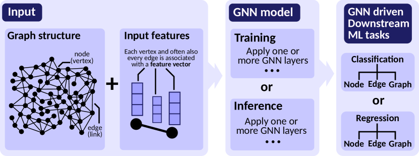
Figure 1: (§ 2.1) Overview of general GNN computation. Input comprises the graph structure and the accompanying feature vectors (assigned to vertices/edges). The input is processed using a specific GNN model (training or inference). Output feature vectors are used in various downstream ML tasks.

We overview a GNN computation in Figure 1. The input is a graph dataset, which can be a single graph (usually a large one, e.g., a brain network), or several graphs (usually many small ones, e.g., chemical molecules). The input usually comes with input feature vectors that encode the semantics of a given task. For example, if the input nodes and edges model – respectively – papers and citations between these papers, then each node could come with an input feature vertex being a one-hot bag-of-words encoding, specifying the presence of words in the abstract of a given publication. Then, a GNN model – underlying the training and inference process – uses the graph structure and the input feature vectors to generate the output feature vectors. In this process, intermediate hidden latent vectors are often created. Note that hidden features may be updated iteratively more than once (we refer to a single such iteration, that updates all the hidden features, as a GNN layer). The output feature vectors are then used for the downstream ML tasks such as node classification or graph classification.

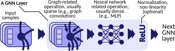
Figure 2: (§ 2.1) Overview of one GNN layer. The input samples (e.g., vertices or graphs) are processed with a graph-related operation such as graph convolution, followed by a neural network related operation such as an MLP, then optionally by a non-linearity such as ReLU, and potentially by some normalization.

A single GNN layer is summarized in Figure 2. In general, one first applies a certain graph-related operation to the features. For example, in the GCN model [131], one aggregates the features of neighbors of each vertex $v$ into the feature vector of $v$ using summation. Then, a selected operation related to traditional neural networks is applied to the feature vectors. A common choice is an MLP or a plain linear projection. Finally, one often uses some form of non-linear activation (e.g., ReLU [131]) and/or normalization.

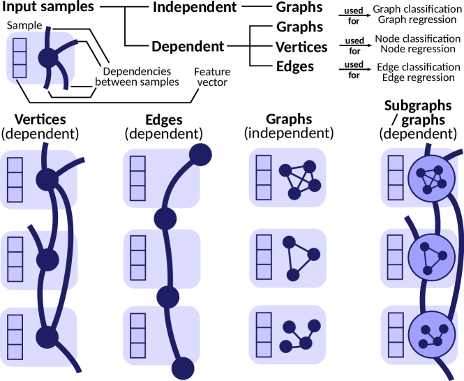
Figure 3: (§ 2.1) Overview of GNN samples. GNN downstream ML tasks aim at classification or regression of vertices, edges, or graphs. While both vertex and edge samples virtually always have inter-sample dependencies, graphs may be both dependent and independent.

One key difference between GNNs and traditional deep learning are possible dependencies between input data samples which make the parallelization of GNNs much more challenging. We show GNN data samples in Figure 3. A single sample can be a node (a vertex), an edge (a link), a subgraph, or a graph itself. One may aim to classify samples (assign labels from a discrete set) or conduct regression (assign continuous values to samples). Both vertices and edges have inter-dependencies: vertices are connected with edges while edges share common vertices. The seminal work by Kipf and Welling [131] focuses on node classification. Here, one is given a single graph as input, data samples are single vertices, and the goal is to classify all unlabeled vertices.

Graphs – when used as basic data samples – are usually independent [242, 236] (cf. Figure 3, 3rd column). An example use case is classifying chemical molecules. This setting resembles traditional deep learning (e.g., image recognition), where samples (single pictures) also have no explicit dependencies. Note that, as chemical molecules may differ in sizes, load balancing issues may arise (we discuss it in Section 3.2). This also has analogies in traditional deep learning, e.g., sampled videos also may have varying sizes [146]. Graph classification may also feature graph samples with inter-dependencies (cf. Figure 3, 4th column). This is useful when studying, for example, relations between network communities [145]; see Section 3.2 for details.

We illustrate examples and taxonomy of GNN tasks in Figure 4.

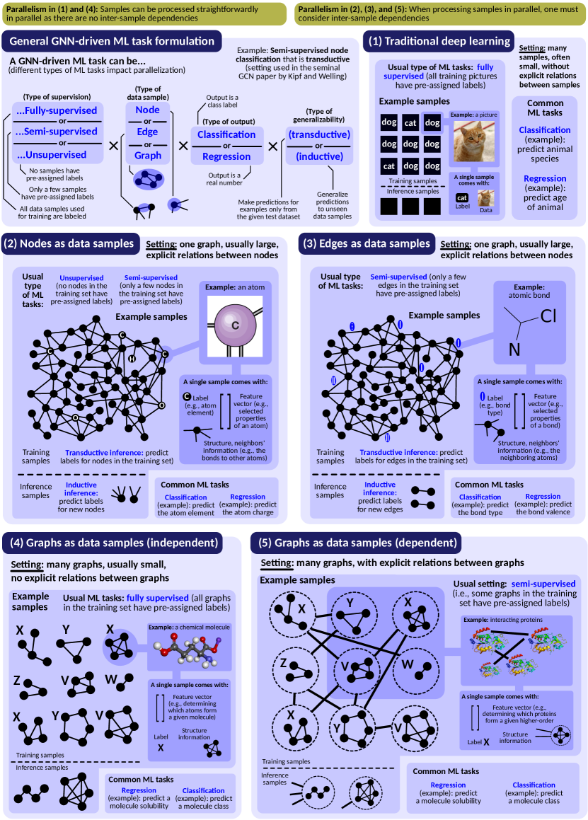
Figure 4: Examples and taxonomy of GNN tasks.

2.2 Input Datasets & Output Structures in GNNs

A GNN computation starts with the input graph $G$, modeled as a tuple $(V,E)$; $V$ is a set of vertices and $E\subseteq V\times V$ is a set of edges; $|V|=n$ and $|E|=m$. $N(v)$ denotes the set of vertices adjacent to vertex (node) $v$, $d_{v}$ is $v$’s degree, and $d$ is the maximum degree in $G$ (all symbols are listed in Table I). The adjacency matrix (AM) of a graph is $\mathbf{A}\in\{0,1\}^{n\times n}$. $\mathbf{A}$ determines the connectivity of vertices: $\mathbf{A}(i,j)=1\Leftrightarrow(i,j)\in E$. The input, output, and hidden feature vector of a vertex $i$ are denoted with, respectively, $\mathbf{x}_{i},\mathbf{y}_{i},\mathbf{h}_{i}$. We have $\mathbf{x}_{i}\in\mathbb{R}^{k}$ and $\mathbf{y}_{i},\mathbf{h}_{i}\in\mathbb{R}^{O(k)}$, where $k$ is the number of input features. These vectors can be grouped in matrices, denoted respectively as $\mathbf{X},\mathbf{Y},\mathbf{H}\in\mathbb{R}^{n\times O(k)}$. If needed, we use the iteration index $(l)$ to denote the latent features in an iteration (GNN layer) $l$ ($\mathbf{h}^{(l)}_{i}$, $\mathbf{H}^{(l)}$). Sometimes, for clarity of equations, we omit the index $(l)$.

2.3 GNN Mathematical Models

A GNN model defines a mathematical transformation that takes as input (1) the graph structure $\mathbf{A}$ and (2) the input features $\mathbf{X}$, and generates the output feature matrix $\mathbf{Y}$. Unless specified otherwise, $\mathbf{X}$ models vertex features. The exact way of constructing $\mathbf{Y}$ based on $\mathbf{A}$ and $\mathbf{X}$ is an area of intense research. Here, hundreds of different GNN models have been developed [234, 265, 258, 58, 102, 49, 255]. Importantly for parallel and distributed execution, one can formulate most GNN models using either the local formulation (LC) based on functions operating on single edges or vertices, or the global formulation (GL), based on operations on matrices grouping all vertex- and edge-related vectors.

2.3.1 GNN Formulations: Local (LC) vs. Global (GL)

We explicitly distinguish LC and GL formulations because they have different potential for performance optimizations. GL formulations can harness techniques from linear algebra and matrix computations, such as communication avoidance [139, 196]. They also offer more potential for vectorization, as one operates on whole feature and adjacency matrices and not on individual feature vectors. LC formulations also have potential advantages. For example, functions operating on single vertices/edges can be programmed more effectively and scheduled more flexibly on low-end compute resources such as serverless functions. Moreover, the fine-grained perspective facilitates integration with vertex-centric graph processing paradigms, benefiting from established parallel frameworks such as Galois [136].

It is often highly non-trivial to provide both an LC and a GL variant of a GNN model. While some models have both formulations (e.g., GCN, GIN, Vanilla Attention, CommNet; cf. Table V), for most models, this is not the case. Many models only have known local formulations (e.g., MoNet, GAT, AGNN, G-GCN, the “pooling” variant of GraphSAGE, EdgeConv “choice 5”; cf. Table V) or global ones (e.g., SGC, ChebNet, DCNN, GDC, LINE, PPNP; cf. Table VII). Very often, developing an LC variant of a GL model is hard, e.g., for the PPNP model, it would require finding the LC equivalent of inverting the adjacency matrix. On the other hand, complex operations used to compute a score for an edge in many LC formulations (e.g., in MoNet or G-GCN) are challenging to express in GL formulations. Hence, it is important to investigate both types of formulations to ensure all these models can benefit from efficient parallel and distributed execution.

Figure 5 shows the taxonomy of GNN formulations. The LC sub-categories were proposed by Bronstein et al. [48]; the GL sub-categories are described by Chen et al. [63].

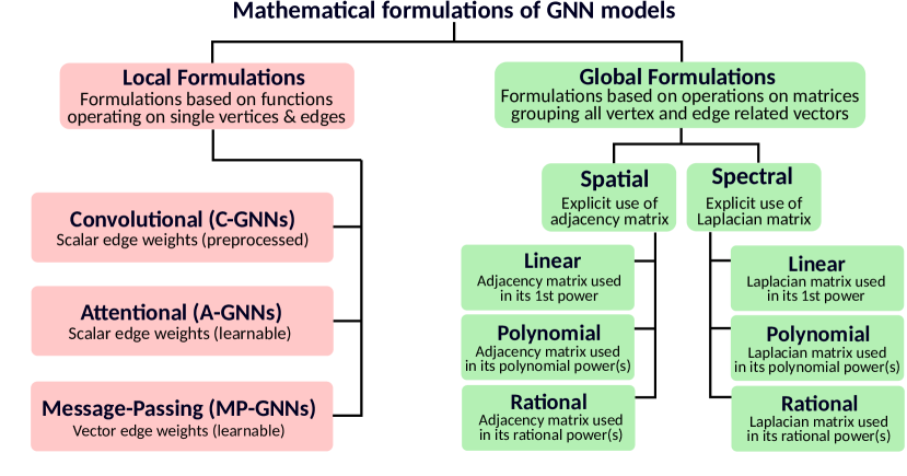
Figure 5: (§ 2.3) Categories of GNN models. We classify the GNN model formulations into local and global. Red/green refer to formulation details in Figure 6.

2.3.2 Local GNN Formulations: Details

In many GNN models, the latent feature vector $\mathbf{h}_{i}$ of a given node $i$ is obtained by applying a permutation invariant aggregator function $\bigoplus$, such as sum or max, over the feature vectors of the neighbors $N(i)$ of $i$ ($N(i)$ is defined as the 1-hop neighborhood) [48]. Moreover, the feature vector of each neighbor of $i$ may additionally be transformed by a function $\psi$. Finally, the outcome of $\bigoplus$ may be also transformed with another function $\phi$. The sequence of these three transformations forms one GNN layer. We denote such a GNN model formulation (based on $\bigoplus,\psi,\phi$) as local (LC). Formally, the equation specifying the feature vector $\mathbf{h}^{(l+1)}_{i}$ of a vertex $i$ in the next GNN layer $l+1$ is as follows:

$$\mathbf{h}^{(l+1)}_{i}=\phi\left(\mathbf{h}^{(l)}_{i},\bigoplus_{j\in N(i)}\psi\left(\mathbf{h}^{(l)}_{i},\mathbf{h}^{(l)}_{j}\right)\right)$$ (1)

As an example, consider the seminal GCN model by Kipf and Welling [131]. Here, $\bigoplus$ is a sum over $N(i)\cup\{i\}\equiv\widehat{N}(i)$, $\psi$ acts on each neighbor $j$’s feature vector by multiplying it with a scalar $1/\sqrt{d_{i}d_{j}}$, and $\phi$ is a linear projection with a trainable parameter matrix $\mathbf{W}$ followed by $ReLU$. Thus, the LC formulation is given by $\mathbf{h}_{i}^{(l+1)}=ReLU\left(\mathbf{W}^{(l)}\times\left(\sum_{j\in\widehat{N}(i)}\frac{1}{\sqrt{d_{i}d_{j}}}\mathbf{h}_{j}^{(l)}\right)\right)$. Note that each iteration may have different projection matrices $\mathbf{W}^{(l)}$.

Depending on the details of $\psi$, one can further distinguish three GNN classes [48]: Convolutional GNNs (C-GNNs), Attentional GNNs (A-GNNs), and Message-Passing GNNs (MP-GNNs). Example models from each class can be found in Table V. In short, in these three classes of models, $\psi$ respectively applies – as a weight on the features – a fixed scalar coefficient (C-GNNs), a learnable scalar coefficient (A-GNNs), or a learnable vector coefficient (MP-GNNs).

Importantly, these approaches form a hierarchy, i.e., C-GNNs $\subseteq$ A-GNNs $\subseteq$ MP-GNNs [48]. Specifically, A-GNNs can represent C-GNNs by implementing attention as a look-up table $a(x_{u},x_{v})=c_{uv}$. Then, both C-GNNs and A-GNNs are special cases of MP-GNNs: $\psi(x_{u},x_{v})=c_{uv}\psi(x_{v})$ (for GNNs) and $\psi(x_{u},x_{v})=a(x_{u},x_{v})\psi(x_{v})$ for A-GNNs.

Note that we follow the taxonomy established by Bronstein et al. [48, 175], where MP-GNNs is a parent class of C-GNNs, A-GNNs, but also more specialized message-passing model classes such as MPNN by Gilmer et al. [93] or Graph Networks by Battaglia et al. [14].

There are many ways in which one can parallelize GNNs in the LC formulation. Here, the first-class citizens are “fine-grained” functions being evaluated for vertices and edges. Thus, one could execute these functions in parallel over different vertices, edges, and graphs, parallelize a single function over the feature dimension or over the graph structure, pipeline a sequence of functions within a GNN layer or across GNN layers, or fuse parallel execution of functions. We discuss all these aspects in the following sections.

2.3.3 Global GNN Formulations: Details

Many GNN models can also be formulated using operations on matrices $\mathbf{X}$, $\mathbf{H}$, $\mathbf{A}$, and others. We will refer to this approach as the global (GL) linear algebraic approach.

For example, the GL formulation of the GCN model is $\mathbf{H}^{(l+1)}=ReLU(\mathbf{\widehat{A}}\mathbf{H}^{(l)}\mathbf{W}^{(l)})$. $\mathbf{\widehat{A}}$ is the normalized adjacency matrix with self loops $\mathbf{\widetilde{A}}$ (cf. Table I): $\mathbf{\widehat{A}}=\mathbf{\widetilde{D}}^{-\frac{1}{2}}\mathbf{\widetilde{A}}\mathbf{\widetilde{D}}^{-\frac{1}{2}}$. This normalization incorporates coefficients $1/\sqrt{d_{i}d_{j}}$ shown in the LC formulation above (the original GCN paper gives more details about normalization).

Many GL models use higher powers of $\mathbf{A}$ (or its normalizations). Based on this criterion, GL models can be linear (L) (if only the 1st power of $\mathbf{A}$ is used), polynomial (P) (if a polynomial power is used), and rational (R) (if a rational power is used) [63]. This aspect impacts how to best parallelize a given model, as we illustrate in Section 4. For example, the GCN model [131] is linear.

Importantly, GNN computations involve both sparse and dense matrices. As the performance patterns of operations on such matrices differ vastly [126, 138, 137, 139], this comes with potential for different parallelization routines. We analyze this in more detail in Section 4.

2.4 GNN Inference vs. GNN Training

A series of GNN layers stacked one after another, as detailed in Figure 2 and in § 2.3, constitutes GNN inference. GNN training consists of three parts: forward pass, loss computation, and backward pass. The forward pass has the same structure as GNN inference. For example, in classification, the loss $\mathcal{L}$ is obtained as follows: $\mathcal{L}=\frac{1}{|\mathcal{Y}|}\sum_{i\in\mathcal{Y}}\text{loss}\left(\mathbf{y}_{i},\mathbf{t}_{i}\right)$, where $\mathcal{Y}$ is a set of all the labeled samples, $\mathbf{y}_{i}$ is the final prediction for sample $i$, and $\mathbf{t}_{i}$ is the ground-truth label for sample $i$. In practice, one often uses the cross-entropy loss [65]; other functions may also be used [101].

Backpropagation outputs the gradients of all the trainable weights in the model. A standard chain rule is used to obtain mathematical formulations for respective GNN models. For example, the gradients for the first GCN layer, assuming a total of two layers ($L=2$), are as follows [207]:

$$\gradient_{\mathbf{W}^{(0)}}\mathcal{L}=\left(\mathbf{\widehat{A}}\mathbf{X}\right)^{T}\left(\sigma^{\prime}\left(\mathbf{\widehat{A}}\mathbf{X}\mathbf{W}^{(0)}\right)\odot\mathbf{\widehat{A}}^{T}\text{loss}\left(\mathbf{Y}-\mathbf{T}\right){\mathbf{W}^{(1)}}^{T}\right)$$

where $\mathbf{T}$ is a matrix grouping all the ground-truth vertex labels, cf. Table I for other symbols. This equation reflects the forward propagation formula (cf. § 2.3.3); the main difference is using transposed matrices (because backward propagation involves propagating information in the reverse direction on the input graph edges) and the derivative of the non-linearity $\sigma^{\prime}$.

The structure of backward propagation depends on whether full-batch or mini-batch training is used. Parallelizing mini-batch training is more challenging due to the inter-sample dependencies, we analyze it in Section 3.

2.5 GNN Programming Models and Operators

Recent works that originated in the systems community come with programming and execution models. These models facilitate GNN computations. In general, they each provide a set of programmable kernels, aka operators (also referred to as UDFs – User Defined Functions) that enable implementing the GNN functions both in the LC formulation ($\bigoplus,\psi,\phi$) and in the GL formulation (matrix products and others). Figure 6 shows both LC and GL formulations, and how they translate to the programming kernels.

The most widespread programming/execution model is SAGA [157] (“Scatter-ApplyEdge-Gather-ApplyVertex”), used in many GNN libraries [260]. In the Scatter operator, the feature vectors of the vertices $u,v$ adjacent to a given edge $(u,v)$ are processed (e.g., concatenated) to create the data specific to the edge $(u,v)$. Then, in ApplyEdge, this data is transformed (e.g., passed through an MLP). Scatter and ApplyEdge together implement the $\psi$ function. Then, Gather aggregates the outputs of ApplyEdge for each vertex, using a selected commutative and associative operation. This enables implementing the $\bigoplus$ function. Finally, ApplyVertex conducts some user specified operation on the aggregated vertex vectors (implementing $\phi$).

Note that, to express the edge related kernels Scatter and UpdateEdge, the LC formulation provides a generic function $\psi$. On the other hand, to express these kernels in the GL formulation, one adds an element-wise product between the adjacency matrix $\mathbf{A}$ and some other matrix being a result of matrix operations that provide the desired effect. For example, to compute a “vanilla attention” model on graph edges, one uses a product of $\mathbf{H}^{(l)}$ with itself transposed.

Other operators, proposed in GReTA [129], FlexGraph [218], and others, are similar. For example, GReTA has one additional operator, Activate, which enables a separate specification of activation. On the other hand, GReTA does not provide a kernel for applying the $\psi$ function.

We illustrate the relationships between operators and GNN functions from the LC and GL formulations, in Figure 6. Here, we use the name Aggregate instead of Gather to denote the kernel implementing the $\bigoplus$ function. This is because “Gather” has traditionally been used to denote bringing several objects together into an array [165].

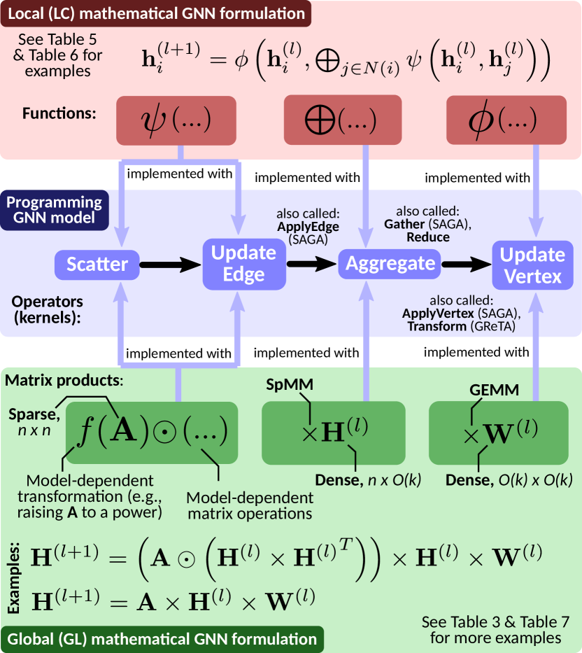
Figure 6: (§ 2.3–§ 2.5) GNN model formulations (top part: the local (LC) approach, bottom part: the global (GL) approach), and how they translate into GNN operators (central part). SAGA [157], NAU [218], and GReTA [129] are GNN programming models. Red/green indicate formulations from Figure 5.

Parallelism in these programming and execution models is tightly related to that of the associated GNN functions in LC and GL formulations; we discuss it in Section 4. We also analyze parallel and distributed frameworks and accelerators based on these models in Section 5.

2.6 Taxonomy of Parallelism in GNNs

In traditional DL, there are two fundamental ways to parallelize the processing of a neural network [16]: data parallelism and model parallelism where one partitions, respectively, data samples and neural weights among different workers. Parallelism in GNNs also has data parallelism (detailed in Section 3) and model parallelism (detailed in Section 4). Yet, there are certain differences that we identify and analyze. We overview the GNN parallelism taxonomy and the classes of GNN parallelism in Figure 7 and 8, respectively.

Figure 7: (§ 2.6) Parallelism taxonomy in GNNs.

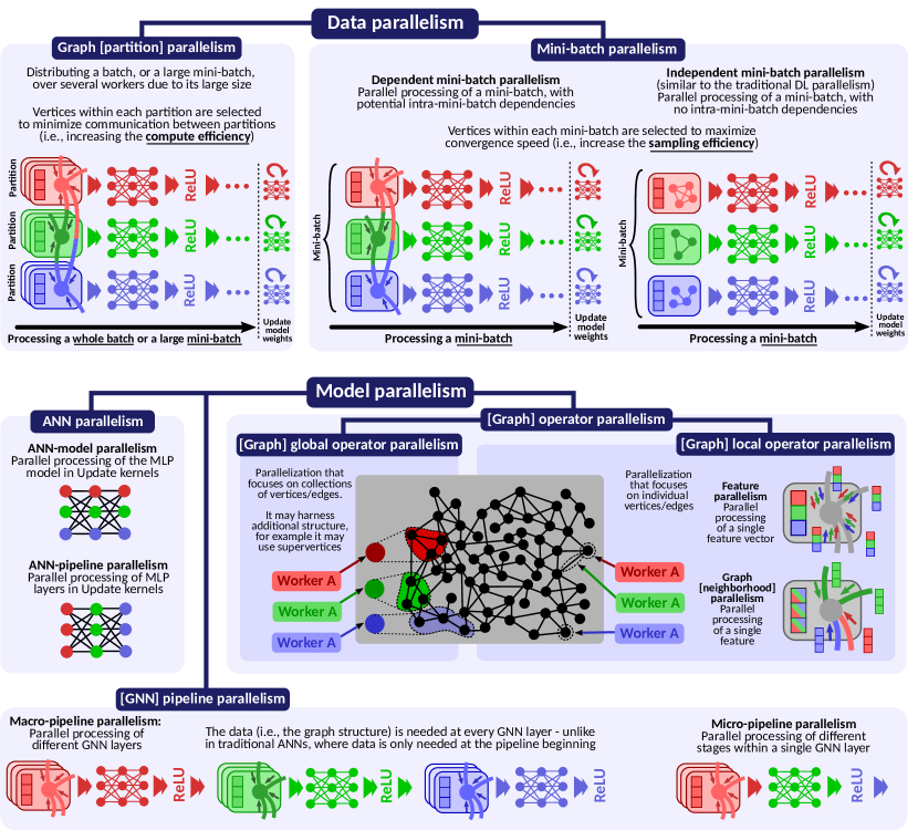
Figure 8: (§ 2.6) Overview of parallelism in GNNs. Different colors (red, green, blue) correspond to different workers.

The first form of data parallelism in GNNs is independent mini-batch parallelism. Here, parallel workers process a single mini-batch; the samples in this mini-batch have no inter-sample dependencies (i.e., the samples are independent graphs, see Figure 3). This form of parallelism is analogous to the one in deep learning with images, where one parallelizes a mini-batch of pictures. Second, GNNs also exhibit dependent mini-batch parallelism. Here, a mini-batch is also processed in parallel by multiple workers, but the samples do have inter-sample dependencies (e.g., a mini-batch could be a set of vertices and edges, sampled from a large input graph). These dependencies make parallelization much more complex, as we detail in Section 3. Note that in GNNs, as in traditional DL, one can also use full-batch training. Finally, one can combine both mini-batch parallelism and full-batch processing with graph [partition] parallelism. Here, one distributes a given mini-batch or a whole batch across different workers, usually to fit it in memory.

Model parallelism in GNNs can be divided into operator parallelism, artificial neural network (ANN) parallelism, and pipeline parallelism. First, in operator parallelism, one parallelizes the Scatter and Reduce kernels. Here, we further distinguish between [graph] local operator parallelism (parallel processing of individual vertices and edges) and [graph] global operator parallelism (parallel processing of collections of vertices/edges). Examples of local operator parallelism are feature parallelism (processing a feature vector of a given vertex in parallel) and graph [neighborhood] parallelism (processing in parallel the edges to the neighbors of a given vertex). Second, in ANN parallelism, one parallelizes the UpdateEdge and UpdateVertex kernels. These kernels can harness any form of parallelism that has been developed for traditional deep neural networks such as MLPs [16]. Examples of ANN parallelism are ANN-pipeline parallelism (pipelining MLP layers) and ANN-operator parallelism (parallel processing of single NN operations). Finally, in [GNN] pipeline parallelism, one assigns different workers to different stages of the GNN processing pipeline. Here, we distinguish macro-pipeline parallelism (pipelining the whole GNN layers) and micro-pipeline parallelism (pipelining the stages within a single GNN layer).

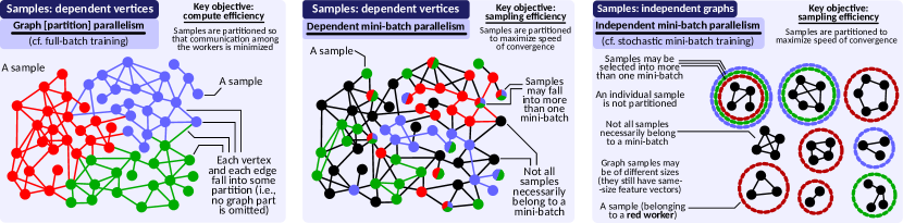
Figure 9: (§ 3.1, § 3.2) Graph partition parallelism vs. dependent and independent mini-batch parallelism in GNNs. Different colors (red, green, blue) indicate different graph partitions or mini-batches, and the associated different workers. Note that applying different colors to a vertex or to an independent graph does not mean physical partitioning but it indicates that a given vertex or a given indepedent graph – as a whole – is used in more than a single mini-batch, indicated by the respective color. Black vertices do not belong to any mini-batch.

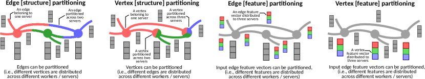
Figure 10: (§ 3.1) Different forms of graph partition parallelism. Different colors (red, green, blue) indicate different graph partitions, and the associated different workers. The gray graph element is oblivious to a given form of partitioning. Note that different partitioning schemes can be combined together.

2.7 Parallel and Distributed Models and Algorithms

We use formal models for reasoning about parallelism. For a single-machine (shared-memory), we use the work-depth (WD) analysis, an established approach for bounding run-times of parallel algorithms. The work of an algorithm is the total number of operations and the depth is defined as the longest sequential chain of execution in the algorithm (assuming infinite number of parallel threads executing the algorithm), and it forms the lower bound on the algorithm execution time [39, 42]. One usually wants to minimize depth while preventing work from increasing too much.

In multi-machine (distributed-memory) settings, one is often interested in understanding the algorithm cost in terms of the amount of communication (i.e., communicated data volume), synchronization (i.e., the number of global “supersteps”), and computation (i.e., work), and minimizing these factors. A popular model used in this setting is Bulk Synchronous Parallel (BSP) [210].

3 Data Parallelism

In traditional deep learning, a basic form of data parallelism is to parallelize the processing of input data samples within a mini-batch. Each worker processes its own portion of samples, computes partial updates of the model weights, and synchronizes these updates with other workers using established strategies such as parameter servers or allreduce [16]. As samples (e.g., pictures) are independent, it is easy to parallelize their processing, and synchronization is only required when updating the model parameters. In GNNs, mini-batch parallelism is more complex because very often, there are dependencies between data samples (cf. Figure 3 and § 2.1. Moreover, the input datasets as a whole are often massive. Thus, regardless of whether and how mini-batching is used, one is often forced to resort to graph partition parallelism because no single server can fit the dataset. We now detail both forms of GNN data parallelism. We illustrate them in Figure 9.

3.1 Graph Partition Parallelism

Some graphs may have more than 250 billion vertices and beyond 10 trillion edges [150, 18], and each vertex and/or edge may have a large associated feature vector [112]. Thus, one inevitably must distribute such graphs over different workers as they do not fit into one server memory. We refer to this form of GNN parallelism as the graph partition parallelism, because it is rooted in the established problem of graph partitioning [51, 125] and the associated mincut problem [92, 125, 85]. The main objective in graph partition parallelism is to distribute the graph across workers in such a way that both communication between the workers and work imbalance among workers are minimized.

We illustrate variants of graph partitioning in Figure 10. When distributing a graph over different workers and servers, one can specifically distribute vertices (edge [structure] partitioning, i.e., edges are partitioned), edges (vertex [structure] partitioning, i.e., vertices are partitioned), or edge and/or vertex input features (edge/vertex [feature] partitioning, i.e., edge and/or vertex input feature vectors are partitioned). Importantly, these methods can be combined, e.g., nothing prevents using both edge and feature vector partitioning together. Edge partitioning is probably the most widespread form of graph partitioning, but it comes with large communication and work imbalance when partitioning graphs with skewed degree distributions. Vertex partitioning alleviates it to a certain degree, but if a high-degree vertex is distributed among many workers, it also incurs overheads in maintaining a consistent distributed vertex state. Differences between edge and vertex partitioning are covered extensively in rich literature [55, 73, 96, 51, 125, 73, 52, 50, 9, 127, 75, 106, 124]. Feature vertex partitioning was not addressed in the graph processing area because in traditional distributed graph algorithms, vertices and/or edges are usually associated with scalar values.

Partitioning entails communication when a given part of a graph depends on another part kept on a different server. This may happen during a graph related operator (Scatter, Aggregate) if edges or vertices are partitioned, and during a neural network related operator (UpdateEdge, UpdateVertex) if feature vectors are partitioned.

Partition parallelism usually does not allow a single vertex to belong to multiple partitions (unlike mini-batch parallelism, where a single sample may belong to more than one mini-batch). However, there are strategies for reducing communication, in which vertices are cached on remote partitions. Such schemes would involve maintaining multiple copies of a given vertex on several partitions.

Note that, while graph partition is usually conducted once, before training starts, it could also be in principle reapplied during training, to alleviate potential load imbalance (e.g., due to inserting new vertices or edges). Such schemes are an interesting direction for future work.

3.1.1 Full-Batch Training

Graph partition parallelism is commonly used to alleviate large memory requirements of full-batch training. In full-batch training, one must store all the activations for each feature in each vertex in each GNN layer). Thus, a common approach for executing and parallelizing this scheme is using distributed-memory large-scale clusters that can hold the massive input datasets in their combined memories, together with graph partition parallelism. Still, using such clusters may be expensive, and it still does not alleviate the slow convergence. Hence, mini-batching is often used.

3.2 Mini-Batch Parallelism

In GNNs, if data samples are independent graphs, then mini-batch parallelism is similar to traditional deep learning. First, one mini-batch is a set of such graph samples, with no dependencies between them. Second, samples (e.g., molecules) may have different sizes. This may cause load imbalance), similarly to, e.g., videos [146]. For example, a single dataset (e.g., ChemInformatics) [182] may contain graphs both 5 vertices and 18 edges as well as with 121 vertices and 298 edges. This setting is common in graph classification or graph regression. We illustrate this in Figure 9 (right), and we refer to it as independent mini-batch parallelism. Note that – while graph samples may have different sizes (e.g., molecules can have different counts of atoms and bonds) – their feature counts are the same.

Still, in most GNN computations, mini-batch parallelism is much more challenging because of inter-sample dependencies (dependent mini-batch parallelism). As a concrete example, consider node classification. Similarly to graph partition parallelism, one may experience load imbalance issues, e.g., because vertices may differ in their degrees. Several works alleviate this [201, 162].

While the graph prediction setting has been explored in data science works [227, 83, 112, 77, 234, 237], it has been largely unaddressed in system design studies [1]. As such, to the best of our knowledge, there are no detailed existing load balancing studies or schemes for independent mini-batch parallelism (unlike for node or edge predictions [1]). Dependent mini-batch parallelism with graphs as samples is even more scarcely researched; for example, it does not even have a representing dataset in the Large-Scale OGB challenge [112]. Hence, we list these as research opportunities in Section 8.

Another key challenge in GNN mini-batching is the information loss when selecting the target vertices forming a given mini-batch. In traditional deep learning, one picks samples randomly. In GNNs, straightforwardly applying such a strategy would result in very low accuracy. This is because, when selecting a random subset of nodes, this subset may not even be connected, but most definitely it will be very sparse and due to the missing edges, a lot of information about the graph structure is lost during the Aggregate or Scatter operator. This information loss challenge was circumvented in the early GNN works with full-batch training [131, 234] (cf. § 3.1.1). Unfortunately, full-batch training comes with slow convergence (because the model is updated only once per epoch, which may require processing billions of vertices), and the above-mentioned large memory requirements. Hence, two recent approaches that address specifically mini-batching proposed sampling neighborhoods, and appropriately selecting target vertices.

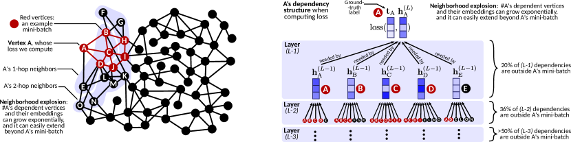
Figure 11: (§ 3.2) Neighborhood explosion in mini-batching in GNNs. This phenomenon is characteristic to schemes based on node-wise sampling [271].

3.2.1 Neighborhood Sampling

In a line of works initiated by GraphSAGE [103], one adds sampled neighbors of each selected target vertex $v$ to the mini-batch. These neighbors are used to increase the accuracy of predictions for target vertices (i.e., they are not used as target vertices in that mini-batch). Specifically, when executing the Scatter and Aggregate kernels for each of target vertices in a mini-batch, one also considers the pre-selected neighbors. Hence, the results of Scatter and Aggregate are more accurate. Sampled neighbors of $v$ usually come from not only 1-hop, but also from $H$-hop neighborhoods of $v$, where $H$ may be as large as graph’s diameter. The exact selection of sampled neighbors depends on the details of each scheme. In GraphSAGE, they are sampled (for each target vertex) for each GNN layer before the actual training.

We illustrate neighborhood sampling in Figure 12. Here, note that the target vertices within each mini-batch may be clustered but may also be spread across the graph (depending on a specific scheme [142, 103, 60, 61]). Sampled neighbors, indicated with darker shades of each mini-batch color, are located up to 2 hops away from their target vertices.

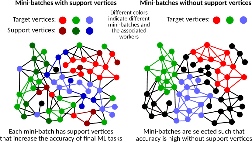
Figure 12: (§ 3.2) Two variants of mini-batching: with and w/o support vertices. Light colors (red, green, blue) indicate different mini-batches (target vertices) and the associated workers. Dark colors (dark red, dark green, dark blue) indicate support vertices for each respective mini-batch. Black vertices do not belong to any mini-batch. Example schemes: GraphSAGE [103] (left), Cluster-GCN [65] (right).

One challenge related to neighborhood sampling is the overhead of their pre-selection. For example, in GraphSAGE, one has to – in addition to the forward and backward propagation passes – conduct as many sampling steps as there are layers in a GNN, to conduct sampling for each layer and for each target vertex. While this can be alleviated with parallelization schemes also used for forward and backward propagation, it inherently increases the depth of a GNN computation by a multiplicative constant factor.

Another associated challenge is called the neighborhood explosion and is related to the memory overhead due to maintaining potentially many such vertices. In the worst case, for each vertex in a mini-batch, assuming keeping all its neighbors up to $H$ hops, one has to maintain $O(kd^{H})$ state. Even if some of these vertices are target vertices in that mini-batch and thus are already maintained, when increasing $H$, their ratio becomes lower. GraphSAGE alleviates this by sampling a constant fraction of vertices from each neighborhood instead of keeping all the neighbors, but the memory overhead may still be large [247]. Other works also explore efficient sampling to avoid neighborhood explosion. For example, shaDow-GNN focuses on extracting a small number of critical neighbors, while excluding irrelevant ones [245]. We show an example neighborhood explosion in Figure 11.

3.2.2 Appropriate Selection of Target Vertices

More recent GNN mini-batching works focus on the appropriate selection of target nodes included in mini-batches, such that support vertices are not needed for high accuracy. For example, Cluster-GCN first clusters a graph and then assigns clusters to mini-batches [65, 241]. This way, one reduces the loss of information because a mini-batch usually contains a tightly knit community of vertices. We illustrate this in Figure 12 (right). However, one has to additionally compute graph clustering as a form of preprocessing. This can be parallelized with one of many established parallel clustering routines [125, 24, 23, 22].

3.3 Graph Partitions vs. Mini-Batch/Full-Batch Training

Graph partitions are used primarily to contain the graph fully in memory (avoiding expensive disk accesses), while mini-batches are used to speed up convergence. The first fundamental difference between these two is the key objective when splitting the graph dataset across workers. For graph partition parallelism, one aims to maximize compute efficiency, i.e., minimize runtimes by minimizing the amount of communication between workers. For the former, one focuses on increasing sampling efficiency, i.e., creating mini-batches in such a way that the convergence speed is maximized. With certain schemes, these objectives could result in selecting similar vertices. For example, Cluster-GCN selects dense clusters as mini-batches and such clusters could also be effective graph partitions [65]. However, this is not always the case as other mini-batching schemes do not necessarily focus on dense clusters [155]. Another difference is that, while a single graph partition is processed by a single worker (i.e., multiple workers process multiple partitions), one mini-batch is processed by multiple workers. We also note that one could consider the parallel processing of different mini-batches. This would entail asynchronous GNN training, with model updates being conducted asynchronously. Such a scheme could slow down convergence, but would offer potential for more parallelism.

Commonly, one uses graph partition parallelism with full-batch training [216, 215, 107, 207]. However, in principle, graph partition and mini-batch parallelism are orthogonal to each other, and could thus be used together. For example, a large mini-batch running on workers with not much memory could utilize graph partition parallelism to avoid I/O. Such an approach has also been proposed in traditional DL [199, 172].

Other differences are as follows. First, the primary objective when partitioning a graph is to minimize communication and work imbalance across workers. Contrarily, in mini-batching, one aims at a selection of target vertices that maximizes accuracy. Second, each vertex belongs to some partition(s), but not each vertex is necessarily included in a mini-batch. Third, while mini-batch parallelism has a variant with no inter-sample dependencies, graph partition parallelism nearly always deals with a connected graph and has to consider such dependencies.

3.4 Work-Depth Analysis

We analyze work/depth of different GNN training schemes that use full-batch or mini-batch training, see Table II.

Method	Work & depth in one training iteration
Full-batch training schemes:
Full-batch [131]	$O\left(Lmk+Lnk^{2}\right)$	$O\left(L\log k+L\log d\right)$
Weight-tying [142]	$O\left(Lmk+Lnk^{2}\right)$	$O\left(L\log k+L\log d\right)$
RevGNN [142]	$O\left(Lmk+Lnk^{2}\right)$	$O\left(L\log k+L\log d\right)$
Mini-batch training schemes:
GraphSAGE [103]	$O\left(Lmk+Lnk^{2}+c^{L}nk^{2}\right)$	$O\left(L\log k+L\log c\right)$
VR-GCN [60]	$O\left(Lmk+Lnk^{2}+c^{L}nk^{2}\right)$	$O\left(L\log k+L\log c\right)$
FastGCN [61]	$O\left(Lmk+Lnk^{2}+cLnk^{2}\right)$	$O\left(L\log k+L\log c\right)$
Cluster-GCN [65]	$O\left(W_{pre}+Lmk+Lnk^{2}\right)$	$O\left(D_{pre}+L\log k+L\log d\right)$
GraphSAINT [247]	$O\left(W_{pre}+Lmk+Lnk^{2}\right)$	$O\left(D_{pre}+L\log k+L\log d\right)$

TABLE II: (§ 3.4) Work-depth analysis of GNN training methods. $c$ is the number of vertices sampled per neighborhood or per GNN layer.

First, all methods have a common term in work being $O(Lmk+Lnk^{2})$ that equals the number of layers $L$ times the number of operations conducted in each layer, which is $mk$ for sparse graph operations (Aggregate) and $nk^{2}$ for dense neural network operations (UpdateVertex). This is the total work for full-batch methods. Mini-batch schemes have additional work terms. Schemes based on support vertices (GraphSAGE, VR-GCN, FastGCN) have terms that reflect how they pick these vertices. GraphSAGE and VR-GCN have a particularly high term $O(c^{L}nk^{2})$ due to the neighborhood explosion ($c$ is the number of vertices sampled per neighborhood). FastGCN alleviates the neighborhood explosion by sampling $c$ vertices per whole layer, resulting in $O(cLnk^{2})$ work. Then, approaches that focus on appropriately selecting target vertices (GraphSAINT, Cluster-GCN) do not have the work terms related to the neighborhood explosion. Instead, they have preprocessing terms indicated with $W_{pre}$. Cluster-GCN’s $W_{pre}$ depends on the selected clustering method, which heavily depends on the input graph size ($n$, $m$). GraphSAINT, on the other hand, does stochastic mini-batch selection, the work of which does not necessarily grow with $n$ or $m$.

In terms of depth, all the full-batch schemes depend on the number of layers $L$. Then, in each layer, two bottleneck operations are the dense neural network operation (UpdateVertex, e.g., a matrix-vector multiplication) and the sparse graph operation (Aggregate). They take $O(\log k)$ and $O(\log d)$ depth, respectively. Mini-batch schemes are similar, with the main difference being the $O(\log c)$ instead of $O(\log d)$ term for the schemes based on support vertices. This is because Aggregate in these schemes is applied over $c$ sampled neighbors. Moreover, in Cluster-GCN and GraphSAINT, the neighborhoods may have up to $d$ vertices, yielding the $O(\log d)$ term. They however have the additional preprocessing depth term $D_{pre}$ that depends on the used sampling or clustering scheme.

To summarize, full-batch and mini-batch GNN training schemes have similar depth. Note that this is achieved using graph partition parallelism in full-batch training methods, and mini-batch parallelism in mini-batching schemes. Contrarily, overall work in mini-batching may be larger due to the overheads from support vertices, or additional preprocessing when selecting target vertices using elaborate approaches. However, mini-batching comes with faster convergence and usually lower memory pressure.

3.5 Tradeoff Between Parallelism & Convergence

The efficiency tradeoff between the amount of parallelism in a mini-batch and the convergence speed, controlled with the mini-batch size, is an important part of parallel traditional ANNs [16]. In short, small mini-batches would accelerate convergence but may limit parallelism while large mini-batches may slow down convergence but would have more parallelism. In GNNs, finding the “right” mini-batch size is much more complex, because of the inter-sample dependencies. For example, a large mini-batch consisting of vertices that are not even connected, would result in very low accuracy. On the other hand, if a mini-batch is small but it consists of tightly connected vertices that form a cluster, then the accuracy of the updates based on processing that mini-batch can be high [65].

4 Model Parallelism

In traditional neural networks, models are often large. In GNNs, models ($\mathbf{W}$) are usually small and often fit into the memory of a single machine. However, numerous forms of model parallelism are heavily used to improve throughput; we provided an overview in § 2.6 and in Figure 8.

In the following model analysis, we often picture the used linear algebra objects and operations. For clarity, we indicate their shapes, densities, and dimensions, using small figures, see Table III for a list. Interestingly, GNN models in the LC formulations heavily use dense matrices and vectors with dimensionalities dominated by $O(k)$, and the associated operations. On the other hand, the GL formulations use both sparse and dense matrices of different shapes (square, rectangular, vectors), and the used matrix multiplications can be dense–dense (GEMM, GEMV), dense–sparse (SpMM), and sparse–sparse (SpMSpM). Other operations are elementwise matrix products or rational sparse matrix powers. This rich diversity of operations immediately illustrates a huge potential for parallel and distributed techniques to be used with different classes of models.

Symbol	Description	Used often in
Matrices and vectors
,	Dense vectors, dimensions: $O(k)\times 1$, $1\times O(k)$	LC models
	Dense matrices, dimensions: $O(k)\times O(k)$	GL & LC models
,	Dense matrices, dimensions: $n\times O(k)$, $O(k)\times n$	GL models
	Sparse matrix, dimensions: $n\times n$	GL models
Matrix multiplications (dimensions as stated above)
$\times$	GEMM, dense tall matrix $\times$ dense square matrix	GL models
$\times$	GEMM, dense square matrix $\times$ dense square matrix	GL models
$\times$	GEMM, dense tall matrix $\times$ dense tall matrix	GL models
$\times$	GEMV, dense matrix $\times$ dense vector	LC models
$\times$	SpMM, sparse matrix $\times$ dense matrix	GL models
Elementwise matrix products and other operations
$\odot$ $(...)$	Elementwise product of a sparse matrix and some object	GL models
$\includegraphics[scale={0.4},trim=0.0pt 16.06pt -8.03pt 0.0pt]{M-sp_n-n.pdf}^{x},x\in\mathbb{N}$	SpMSpM, sparse matrix $\times$ sparse matrix	GL models
$\includegraphics[scale={0.4},trim=0.0pt 16.06pt -8.03pt 0.0pt]{M-sp_n-n.pdf}^{x},x\in\mathbb{Z}$	Rational sparse matrix power	GL models
$\cdot$ , $\odot$	Vector dot product, elementwise vector product	LC models
$\includegraphics[scale={0.4},trim=0.0pt 8.03pt -8.03pt 0.0pt]{M-dn_k-1.pdf}\big{\|}\ \includegraphics[scale={0.4},trim=0.0pt 8.03pt -8.03pt 0.0pt]{M-dn_k-1.pdf}$, $\sum$	Vector concatenation, sum of $d$ vectors, $d\leq n$	LC models

TABLE III: Important objects and operations from linear algebra used in GNNs. We assign these operations to specific GNN models in Tables V, VI, and VII.

4.1 Local Operator Parallelism

In local operator parallelism, one focuses on parallelizing executions of Scatter and Gather on individual vertices or edges (i.e., local graph elements). We further structure our investigation by considering separately local operator parallelism over LC and GL GNN model formulations.

4.1.1 Parallelism in LC Formulations of GNN Models

We illustrate generic work and depth equations of LC GNN formulations in Figure 13. Overall, work is the sum of any preprocessing costs $W_{pre}$, post-processing costs $W_{post}$, and work of a single GNN layer $W_{l}$ times the number of layers $L$. In the considered generic formulation in Eq. (8), $W_{l}$ equals to work needed to evaluate $\psi$ for each edge ($mW_{\psi}$), $\bigoplus$ for each vertex ($nW_{\oplus}$), and $\phi$ for each vertex ($nW_{\phi}$). Depth is analogous, with the main difference that the depth of a single GNN layer is a plain sum of depths of computing $\psi$, $\bigoplus$, and $\phi$ (each function is evaluated in parallel for each vertex and edge, hence no multiplication with $n$ or $m$).

Work (generic) $$=W_{pre}+LW_{l}+W_{post}$$

Depth (generic) $$=D_{pre}+LD_{l}+D_{post}$$

Work of Eq. (8) $$=W_{pre}+L\cdot\left(mW_{\psi}+nW_{\oplus}+nW_{\phi}\right)+W_{post}$$

Depth of Eq. (8) $$=D_{pre}+L\cdot\left(D_{\psi}+D_{\oplus}+D_{\phi}\right)+D_{post}$$

Figure 13: Generic equations for work and depth in GNN LC formulations.

We now analyze work and depth of many specific GNN models, by focusing on the three functions forming these models: $\psi$, $\bigoplus$, and $\phi$. The analysis outcomes are in Tables V and VI. We select the representative models based on a recent survey [63]. We also indicate whether a model belongs to the class of convolutional (C-GNN), attentional (A-GNN), or message-passing (MP-GNN) models [175] (cf. § 2.3.2).

Analysis of $\psi$ We show the analysis results in Table V. We provide the formulation of $\psi$ for each model, and we also illustrate all algebraic operations needed to obtain $\psi$. All C-GNN models have their $\psi$ determined during preprocessing. This preprocessing corresponds to the adjacency matrix row normalization ($c_{ij}=1/d_{i}$), the column normalization ($c_{ij}=1/d_{j}$), or the symmetric normalization ($c_{ij}=1/\sqrt{d_{i}d_{j}}$) [234]. In all these cases, their derivation takes $O(1)$ depth and $O(m)$ work. Then, A-GNNs and MP-GNNs have much more complex formulations of $\psi$ than C-GNNs. Details depend on the model, but - importantly - nearly all the models have $O(k^{2})$ work and $O(\log k)$ depth. The most computationally intense model, GAT, despite having its work equal to $O(dk^{2})$, has also logarithmic depth of $O(\log k+\log d)$. This means that computing $\psi$ in all the considered models can be effectively parallelized. As for the sparsity pattern and type of operations involved in evaluating $\psi$, most models use GEMV. All the considered A-GNN models also use transposition of dense vectors. GAT also uses vector concatenation and sum of up to $d$ vectors. Finally, one considered MP-GNN model uses an elementwise MV product. In general, each considered GNN model uses dense matrix and vector operations to obtain $\psi$ for each of the associated edges.

Note that, by default, $\psi$ corresponds to edge feature vectors that are “transient”, i.e., they are computed on the fly and are not stored explicitly (unlike vertex feature vectors). However, in some cases, one may also want to explicitly instantiate edge feature vectors. Such instantiation would be used in, for example, edge classification or edge regression tasks. An example GNN formulation that enables this is Graph Networks by Battaglia et al. [14], also an LC formulation. The insights about parallelism in such a formulation are not different than the ones provided in this section; the main different is the additional memory overhead of $O(mk)$ needed for storing all edge feature vectors.

Analysis of $\bigoplus$ The aggregate operator $\bigoplus_{j\in N(i)}$ is almost always commutative and associative (e.g., min, max, or plain sum [219, 79]). While it operates on vectors $\mathbf{x}_{j}$ of dimensionality $k$, each dimension can be computed independently of others. Thus, to compute $\bigoplus_{j\in N(i)}$, one needs $O(\log d_{i})$ depth and $O(kd_{i})$ work, using established parallel tree reduction algorithms [41]. Hence, $\bigoplus$ is the bottleneck in depth in all the considered models. This is because $d$ (maximum vertex degree) is usually much larger than $k$.

Analysis of $\phi$ The analysis of $\phi$ is shown in Table VI (for the same models as in Table V). We show the total model work and depth. All the models entail matrix-vector dense products and a sum of up to $d$ dense vectors. Depth is logarithmic. Work varies, being the highest for GAT.

We also illustrate the operator parallelism in the LC formulation, focusing on the GNN programming kernels, in the top part of Figure 14. We provide the corresponding generic work-depth analysis in Table IV. The four programming kernels follow the work and depth of the corresponding LC functions ($\psi,\oplus,\phi$).

Kernel	Work	Depth	Comm.	Sync.
Scatter ($\psi$)	$O(1)$	$O(1)$	$O(mk)$	$O(1)$
UpdateEdge ($\psi$)	$O(mW_{\psi})$	$O(D_{\psi})$	$O(1)$	$O(1)$
Aggregate ($\oplus$)	$O(nW_{\oplus})$	$O(D_{\oplus}\log d)$	$O(mk)$	$O(1)$
UpdateVertex ($\phi$)	$O(nW_{\phi})$	$O(D_{\phi})$	$O(1)$	$O(1)$

TABLE IV: Work-depth analysis of GNN operators (kernels).

Reference	Class	Formulation for $\psi\left(\mathbf{h}_{i},\mathbf{h}_{j}\right)$	Dimensions & density of one execution of $\psi\left(\mathbf{h}_{i},\mathbf{h}_{j}\right)$	Pr?	Work & depth of one execution of $\psi\left(\mathbf{h}_{i},\mathbf{h}_{j}\right)$
GCN [131]	C-GNN	$\frac{1}{\sqrt{d_{i}d_{j}}}\mathbf{h}_{j}$	$c$ $\cdot$		$O(k)$	$O(1)$
GraphSAGE [103] (mean)	C-GNN	$\mathbf{h}_{j}$			$O(1)$	$O(1)$
GIN [237]	C-GNN	$\mathbf{h}_{j}$			$O(1)$	$O(1)$
CommNet [202]	C-GNN	$\mathbf{h}_{j}$			$O(1)$	$O(1)$
Vanilla attention [211]	A-GNN	$\left(\mathbf{h}_{i}^{T}\cdot\mathbf{h}_{j}\right)\mathbf{h}_{j}$	( $\cdot$ ) $\cdot$		$O\left(k\right)$	$O(\log k)$
MoNet [163]	A-GNN	$\text{exp}\left(-\frac{1}{2}\left(\mathbf{h}_{j}-\mathbf{w}_{j}\right)^{T}\mathbf{W}_{j}^{-1}\left(\mathbf{h}_{j}-\mathbf{w}_{j}\right)\right)$	exp( $\times$ $\times$ )		$O\left(k^{2}\right)$	$O(\log k)$
GAT [212]	A-GNN	$\frac{\text{exp}\left(\sigma\left(\mathbf{a}^{T}\cdot\left[\mathbf{W}\mathbf{h}_{i}\big{\|}\mathbf{W}\mathbf{h}_{j}\right]\right)\right)}{\sum_{y\in\widehat{N}(i)}\text{exp}\left(\sigma\left(\mathbf{a}^{T}\cdot\left[\mathbf{W}\mathbf{h}_{i}\big{\|}\mathbf{W}\mathbf{h}_{y}\right]\right)\right)}\mathbf{h}_{j}$	$\frac{\text{exp}\bigg{(}\includegraphics[scale={0.4},trim=0.0pt 2.00749pt -8.03pt 0.0pt]{M-dn_1-k.pdf}\cdot\bigg{[}\includegraphics[scale={0.4},trim=0.0pt 8.03pt -8.03pt 0.0pt]{M-dn_k-k.pdf}\times\includegraphics[scale={0.4},trim=0.0pt 8.03pt -8.03pt 0.0pt]{M-dn_k-1.pdf}\bigg{\|}\ \includegraphics[scale={0.4},trim=0.0pt 8.03pt -8.03pt 0.0pt]{M-dn_k-k.pdf}\times\includegraphics[scale={0.4},trim=0.0pt 8.03pt -8.03pt 0.0pt]{M-dn_k-1.pdf}\bigg{]}\bigg{)}}{{\sum}\text{exp}\bigg{(}\includegraphics[scale={0.4},trim=0.0pt 2.00749pt -8.03pt 0.0pt]{M-dn_1-k.pdf}\cdot\bigg{[}\includegraphics[scale={0.4},trim=0.0pt 8.03pt -8.03pt 0.0pt]{M-dn_k-k.pdf}\times\includegraphics[scale={0.4},trim=0.0pt 8.03pt -8.03pt 0.0pt]{M-dn_k-1.pdf}\bigg{\|}\ \includegraphics[scale={0.4},trim=0.0pt 8.03pt -8.03pt 0.0pt]{M-dn_k-k.pdf}\times\includegraphics[scale={0.4},trim=0.0pt 8.03pt -8.03pt 0.0pt]{M-dn_k-1.pdf}\bigg{]}\bigg{)}}\cdot\includegraphics[scale={0.4},trim=0.0pt 8.03pt -8.03pt 0.0pt]{M-dn_k-1.pdf}$		$O\left(dk^{2}\right)$	$O\left(\log k+\log d\right)$
Attention-based GNNs [206]	A-GNN	$w\frac{\mathbf{h}_{i}^{T}\cdot\mathbf{h}_{j}}{\left\lVert\mathbf{h}_{i}\right\rVert\left\lVert\mathbf{h}_{j}\right\rVert}\mathbf{h}_{j}$	( $\cdot$ ) $\cdot$		$O(k)$	$O(\log k)$
G-GCN [47]	MP-GNN	$\sigma\left(\mathbf{W}_{1}\mathbf{h}_{i}+\mathbf{W}_{2}\mathbf{h}_{j}\right)\odot\mathbf{h}_{j}$	( $\times$ ) $\odot$		$O(k^{2})$	$O(\log k)$
GraphSAGE [103] (pooling)	MP-GNN	$\sigma\left(\mathbf{W}\mathbf{h}_{j}+\mathbf{w}\right)$	$\times$		$O(k^{2})$	$O(\log k)$
EdgeConv [226] “choice 1”	MP-GNN	$\mathbf{W}\mathbf{h}_{j}$	$\times$		$O(k^{2})$	$O(\log k)$
EdgeConv [226] “choice 5”	MP-GNN	$\sigma\left(\mathbf{W}_{1}\left(\mathbf{h}_{j}-\mathbf{h}_{i}\right)+\mathbf{W}_{2}\mathbf{h}_{i}\right)$	$\times$		$O(k^{2})$	$O(\log k)$

TABLE V: Comparison of local (LC) formulations of GNN models with respect to the inner function $\psi\left(\mathbf{h}_{i},\mathbf{h}_{j}\right)$. For clarity and brevity of equations, when it is obvious, we omit the matrix multiplication symbol $\times$ and the indices of a given iteration (GNN layer) number $(l)$. “Class”: class of a GNN model with respect to the complexity of $\psi$, details are in Section 2. All models considered in this table feature aggregations over 1-hop neighbors (“Type L”, details are in Section 2). “Dimensions & density”: dimensions and density of the most important tensors and tensor operations when computing $\psi\left(\mathbf{h}_{i},\mathbf{h}_{j}\right)$ in a given model. “Pr”: can coefficients in $\psi$ be preprocessed (), or do they have to be learnt ()? When listing the most important tensor operations, we focus on multiplications.

Reference	Class	Formulation of $\phi$ for $\mathbf{h}^{(l)}_{i}$; $\psi\left(\mathbf{h}_{i},\mathbf{h}_{j}\right)$ are stated in Table V	Dimensions & density of computing $\phi(\cdot)$, excluding $\psi(\cdot)$	Work & depth (a whole training iteration or inference, including $\psi$ from Table V)
GCN [131]	C-GNN	${\mathbf{W}\times\left(\sum_{j\in\widehat{N}(i)}\psi\left(\mathbf{h}_{j}\right)\right)}$	$\times{\sum}$	$O(Lmk+Lnk^{2})$	$O(L\log d+L\log k)$
GraphSAGE [103] (mean)	C-GNN	${\mathbf{W}\times\left(\frac{1}{d_{i}}\cdot\left(\sum_{j\in\widehat{N}(i)}\psi\left(\mathbf{h}_{j}\right)\right)\right)}$	$\times\sum$	$O(Lmk+Lnk^{2})$	$O(L\log d+L\log k)$
GIN [237]	C-GNN	$\text{MLP}\left((1+\epsilon)\mathbf{h}_{i}+\sum_{j\in N(i)}\psi\left(\mathbf{h}_{j}\right)\right)$	$\overbrace{\;\includegraphics[scale={0.4},trim=0.0pt 8.03pt -8.03pt 0.0pt]{M-dn_k-k.pdf}\times...\times\includegraphics[scale={0.4},trim=0.0pt 8.03pt -8.03pt 0.0pt]{M-dn_k-k.pdf}}^{K\text{times}}\times\sum$	$O(Lmk+LKnk^{2})$	$O(L\log d+LK\log k)$
CommNet [202]	C-GNN	$\mathbf{W}_{1}\mathbf{h}_{i}+\mathbf{W}_{2}\times\left(\sum_{j\in N^{+}(i)}\psi\left(\mathbf{h}_{j}\right)\right)$	$\times\sum$	$O(Lmk+Lnk^{2})$	$O(L\log d+L\log k)$
Vanilla attention [211]	A-GNN	$\mathbf{W}\times\left(\sum_{j\in\widehat{N}(i)}\psi\left(\mathbf{h}_{i},\mathbf{h}_{j}\right)\right)$	$\times\sum$	$O(Lmk+Lnk^{2})$	$O(L\log d+L\log k)$
GAT [212]	A-GNN	$\mathbf{W}\times\left(\sum_{j\in\widehat{N}(i)}\psi\left(\mathbf{h}_{i},\mathbf{h}_{j}\right)\right)$	$\times\sum$	$O(Lmdk^{2}+Lnk^{2})$	$O(L\log d+L\log k)$
Attention-based GNNs [206]	A-GNN	$\mathbf{W}\times\left(\sum_{j\in\widehat{N}(i)}\psi\left(\mathbf{h}_{i},\mathbf{h}_{j}\right)\right)$	$\times\sum$	$O(Lmk+Lnk^{2})$	$O(L\log d+L\log k)$
MoNet [163]	A-GNN	$\mathbf{W}\times\left(\sum_{j\in\widehat{N}(i)}\psi\left(\mathbf{h}_{j}\right)\right)$	$\times\sum$	$O(Lmk^{2}+Lnk^{2})$	$O(L\log d+L\log k)$
G-GCN [47]	MP-GNN	$\mathbf{W}\times\left(\sum_{j\in N^{+}(i)}\psi\left(\mathbf{h}_{i},\mathbf{h}_{j}\right)\right)$	$\times\sum$	$O(Lmk^{2}+Lnk^{2})$	$O(L\log d+L\log k)$
GraphSAGE [103] (pooling)	MP-GNN	$\left(\mathbf{W}\times\left(\mathbf{h}_{i}\Big{\|}\left(\max_{j\in N(i)}\psi\left(\mathbf{h}_{i},\mathbf{h}_{j}\right)\right)\right)\right)$	$\times$ ( ∥ ( $\times\sum$ ) )	$O(Lmk^{2}+Lnk^{2})$	$O(L\log d+L\log k)$
EdgeConv [226] “choice 1”	MP-GNN	$\sum_{j\in N^{+}(i)}\psi\left(\mathbf{h}_{j}\right)$	$\sum$	$O(Lmk^{2}+Lnk^{2})$	$O(L\log d+L\log k)$
EdgeConv [226] “choice 5”	MP-GNN	$\max_{j\in N^{+}(i)}\psi\left(\mathbf{h}_{i},\mathbf{h}_{j}\right)$	$\sum$	$O(Lmk^{2}+Lnk^{2})$	$O(L\log d+L\log k)$

TABLE VI: Comparison of local (LC) formulation of GNN models with respect to the outer function $\phi$. For clarity and brevity of equations, when it is obvious, we omit the matrix multiplication symbol $\times$ and the indices of a given iteration number $(l)$; we also omit activations from the formulations (these are elementwise operations, not contributing to work or depth). “Class”: class of a GNN model with respect to the complexity of $\psi$, details are in Section 2. All models considered in this table feature aggregations over 1-hop neighbors (“Type L”, details are in Section 2). “Dimensions & density”: dimensions and density of the most important tensors and tensor operations in a given model when computing $\mathbf{h}^{(l)}_{i}$. When listing the most important tensor operations, we focus on multiplications.

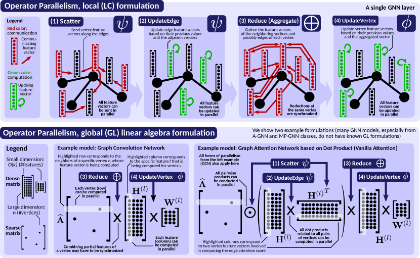
Figure 14: Operator parallelism in GNNs for LC formulations (top) and GL formulations (bottom).

Reference	Type	Algebraic formulation for $\mathbf{H}^{(l+1)}$	Dimensions & density of deriving $\mathbf{H}^{(l+1)}$	#I	Work & depth (one whole training iteration or inference)
GCN [131]	L	$\mathbf{\widehat{A}}\mathbf{H}\mathbf{W}$	$\times$ $\times$	$L$	$O(mkL+Lnk^{2})$	$O(L\log k+L\log d)$
GraphSAGE [103] (mean)	L	$\mathbf{\widehat{A}}\mathbf{H}\mathbf{W}$	$\times$ $\times$	$L$	$O(mkL+Lnk^{2})$	$O(L\log k+L\log d)$
GIN [237]	L	$\text{MLP}\left(((1+\epsilon)\mathbf{I}+\mathbf{\widehat{A}})\mathbf{H}\right)$	$\times$ $\times$ $\times$ … $\times$	$L$	$O(mkL+KLnk^{2})$	$O(LK\log k+LK\log d)$
CommNet [202]	L	$\mathbf{A}\mathbf{H}\mathbf{W}_{2}+\mathbf{H}\mathbf{W}_{1}$	$\times$ $\times$ + $\times$	$L$	$O(mkL+Lnk^{2})$	$O(L\log k+L\log d)$
Dot Product [211]	L	$\left(\mathbf{A}\odot\left(\mathbf{H}{\mathbf{H}}^{T}\right)\right)\mathbf{H}\mathbf{W}$	$\odot$ $\bigg{(}$ $\times$ $\bigg{)}$ $\times$ $\times$	$L$	$O(Lmk+Lnk^{2})$	$O(L\log k+L\log d)$
EdgeConv [226] “choice 1”	L	$\mathbf{A}\mathbf{H}\mathbf{W}$	$\times$ $\times$	$L$	$O(mkL+Lnk^{2})$	$O(L\log k+L\log d)$
SGC [230]	P	$\mathbf{\widehat{A}}^{s}\mathbf{H}\mathbf{W}$	$\includegraphics[scale={0.4},trim=0.0pt 16.06pt -8.03pt 0.0pt]{M-sp_n-n.pdf}^{s}$ $\times$ $\times$	1	$O(mn\log s+nk^{2})$	$O(\log k+\log s\log d)$
DeepWalk [174]	P	$\left(\sum_{s=0}^{T}\mathbf{\overline{A}}^{s}\right)\mathbf{H}\mathbf{W}$	$\bigg{(}$ $\includegraphics[scale={0.4},trim=0.0pt 16.06pt -8.03pt 0.0pt]{M-sp_n-n.pdf}^{0}$ + …+ $\includegraphics[scale={0.4},trim=0.0pt 16.06pt -8.03pt 0.0pt]{M-sp_n-n.pdf}^{T}$ $\bigg{)}$ $\times$ $\times$	1	$O(mn\log T+nk^{2})$	$O(\log k+\log T\log d)$
ChebNet [72]	P	$\left(\sum_{s=0}^{T}\theta_{s}\mathbf{\overline{A}}^{s}\right)\mathbf{H}\mathbf{W}$	$\bigg{(}$ $\includegraphics[scale={0.4},trim=0.0pt 16.06pt -8.03pt 0.0pt]{M-sp_n-n.pdf}^{0}$ + …+ $\includegraphics[scale={0.4},trim=0.0pt 16.06pt -8.03pt 0.0pt]{M-sp_n-n.pdf}^{T}$ $\bigg{)}$ $\times$ $\times$	1	$O(mn\log T+nk^{2})$	$O(\log k+\log T\log d)$
DCNN [6], GDC [133]	P	$\left(\sum_{s=1}^{T}w_{s}\mathbf{\overline{A}}^{s}\right)\mathbf{H}\mathbf{W}$	$\bigg{(}$ $\includegraphics[scale={0.4},trim=0.0pt 16.06pt -8.03pt 0.0pt]{M-sp_n-n.pdf}^{1}$ + …+ $\includegraphics[scale={0.4},trim=0.0pt 16.06pt -8.03pt 0.0pt]{M-sp_n-n.pdf}^{T}$ $\bigg{)}$ $\times$ $\times$	1	$O(mn\log T+nk^{2})$	$O(\log k+\log T\log d)$
Node2Vec [99]	P	$\left(\frac{1}{p}\mathbf{I}+\left(1-\frac{1}{q}\right)\mathbf{\overline{A}}+\frac{1}{q}\mathbf{\overline{A}}^{2}\right)\mathbf{H}\mathbf{W}$	$\bigg{(}$ $\includegraphics[scale={0.4},trim=0.0pt 16.06pt -8.03pt 0.0pt]{M-sp_n-n.pdf}^{0}$ + … + $\includegraphics[scale={0.4},trim=0.0pt 16.06pt -8.03pt 0.0pt]{M-sp_n-n.pdf}^{2}$ $\bigg{)}$ $\times$ $\times$	1	$O(mn+nk^{2})$	$O(\log k+\log d)$
LINE [151], SDNE [217]	P	$\left(\mathbf{\overline{A}}+\theta\mathbf{\overline{A}}^{2}\right)\mathbf{H}\mathbf{W}$	$\bigg{(}$ + $\includegraphics[scale={0.4},trim=0.0pt 16.06pt -8.03pt 0.0pt]{M-sp_n-n.pdf}^{2}$ $\bigg{)}$ $\times$ $\times$	1	$O(mn+nk^{2})$	$O(\log k+\log d)$
Auto-Regress [264, 270]	R	$\left((1+\alpha)\mathbf{I}-\alpha\mathbf{\widehat{A}}\right)^{-1}\mathbf{H}\mathbf{W}$	$\includegraphics[scale={0.4},trim=0.0pt 16.06pt -8.03pt 0.0pt]{M-sp_n-n.pdf}^{-1}$ $\times$ $\times$	1	$O(n^{3}+nk^{2})$	$O(\log^{2}n+\log k)$
PPNP [241, 132, 43]	R	$\alpha\left(\mathbf{I}-(1-\alpha)\mathbf{\widehat{A}}\right)^{-1}\mathbf{H}\mathbf{W}$	$\includegraphics[scale={0.4},trim=0.0pt 16.06pt -8.03pt 0.0pt]{M-sp_n-n.pdf}^{-1}$ $\times$ $\times$	1	$O(n^{3}+nk^{2})$	$O(\log^{2}n+\log k)$
ARMA [38], ParWalks [232]	R	$b\left(\mathbf{I}-a\mathbf{\widehat{A}}\right)^{-1}\mathbf{H}\mathbf{W}$	$\includegraphics[scale={0.4},trim=0.0pt 16.06pt -8.03pt 0.0pt]{M-sp_n-n.pdf}^{-1}$ $\times$ $\times$	1	$O(n^{3}+nk^{2})$	$O(\log^{2}n+\log k)$

TABLE VII: Comparison of global (GL) linear algebra formulations of GNN models. For clarity and brevity of equations, when it is obvious, we omit the matrix multiplication symbol $\times$ and the indices of a given iteration number $(l)$; we also omit activations from the formulations (these are elementwise operations, not contributing to work or depth). “Type”: type of a GNN model with respect to the scope of accessed vertex neighbors, details are in Section 2 (“L”: adjacency matrix is used in its 1st power, “P”: adjacency matrix is used in its polynomial power, “R”: adjacency matrix is used in its rational power). “#I”: the number of GNN layers (GNN iterations). “Dimensions & density”: dimensions and density of the most important tensors and tensor operations in a given model. When listing the most important tensor operations, we focus on multiplications.

Communication & Synchronization Communication in the LC formulations takes place in the Scatter kernel (a part of $\psi$) if vertex feature vectors are communicated to form edge feature vectors; transferred data amounts to $O(mk)$. Similarly, during the Aggregate kernel ($\bigoplus$), there can also be $O(mk)$ data moved. Both UpdateEdge ($\psi$) and UpdateVertex ($\phi$) do not explicitly move data. However, they may be associated with communication intense operations; especially A-GNNs and MP-GNNs often have complex processing associated with $\psi$ and $\phi$, cf. Tables V and VI. While this processing entails matrices of dimensions of up to $O(k)\times O(k)$, which easily fit in the memory of a single machine, this may change in the future, if the feature dimensionality $k$ is increased in future GNN models.

In the default synchronized variants of GNN, computing all kernels of the same type must be followed by global synchronization, to ensure that all data has been received by respective workers (after Scatter and Aggregate) or that all feature vectors have been updated (after UpdateEdge and UpdateVertex). In Section 4.3.3, we discuss how this requirement can be relaxed by allowing asynchronous execution.

4.1.2 Parallelism in GL Formulations of GNN Models

Parallelism in GL formulations is analyzed in Table VII. The models with both LC and FG formulations (e.g., GCN) have the same work and depth. Thus, fundamentally, they offer the same amount of parallelism. However, the GL formulations based on matrix operations come with potential for different parallelization approaches than the ones used for the LC formulations. For example, there are more opportunities to use vectorization, because one is not forced to vectorize the processing of feature vectors for each vertex or edge separately (as in the LC formulation), but instead one could vectorize the derivation of the whole matrix $\mathbf{H}$ [33].

There are also models designed in the GL formulations with no known LC formulations, cf. Tables V–VI. These are models that use polynomial and rational powers of the adjacency matrix, cf. § 2.3.3 and Figure 5. These models have only one iteration. They also offer parallelism, as indicated by the logarithmic depth (or square logarithmic for rational models requiring inverting the adjacency matrix [166]). While they have one iteration, making the $L$ term vanish, they require deriving a given power $x$ of the adjacency matrix $\mathbf{A}$ (or its normalized version). Importantly, as computing these powers is not interleaved with non-linearities (as is the case with many models that only use linear powers of $\mathbf{A}$), the increase in work and depth is only logarithmic, indicating more parallelism. Still, their representative power may be lower, due to the lack of non-linearities.

We overview two example GL models (GCN and vanilla graph attention) in Figure 14 (bottom). In this figure, we also indicate how the LC GNN kernels are reflected in the flow of matrix operations in the GL formulation.

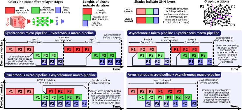
Figure 15: (§ 4.3) Overview of pipelining combined with graph partition parallelism (top-left panel), and of (§ 4.3.3) asynchronous pipelined execution (other panels). Each of four example GNN executions processes three graph partitions (P1, P2, P3) on three stages: red (a sparse graph operation such as convolution), green (a dense neural operation such as MLP), and blue) (a non-linearity such as ReLU). We use two GNN layers (shades indicate layers). The whole execution is fully pipelined, i.e., there are 6 workers in total (three workers for each stage in each layer).

Communication & Synchronization in the GL formulations heavily depend on the used matrix representations and operations. Specifically, there have been a plethora of works into communication reduction in matrix operations, for example targeting dense matrix multiplications [88, 138, 137, 139] or sparse matrix multiplications [198, 195, 196, 94]. They could be used with different GNN operations (cf. Table III) and different models (cf. Table VII). The exact bounds would depend on the selected schemes. Importantly, many works propose to trade more storage for less communication by different forms of input matrix replication [196]. This could be used in GNNs for more performance.

4.1.3 Discussion

Feature vs. Structure vs. Model Weight Parallelism Feature parallelism is straightforward in both LC and GL formulations (cf. Figure 14). In the former, one can execute binary tree reductions over different features in parallel (feature parallelism in $\bigoplus$), or update edge or vertex features in parallel (feature parallelism in $\psi$ and $\phi$). In the latter, one can multiply a row of an adjacency matrix with any column of the latent matrix $\mathbf{H}$ (corresponding to different features) in parallel. As feature vectors are dense, they can be stored contiguously in memory and easily used with vectorization.

Graph neighborhood parallelism is available in both LC and GL formulations. In the former, it is present via parallel execution of $\bigoplus$ (for a single specific feature). In the latter, one parallelizes the multiplication of a given adjacency matrix row with a given feature matrix column.

Traditional model weight parallelism, in which one partitions the weight matrix $\mathbf{W}$ across workers, is also possible in GNNs. Yet, due to the small sizes of weight matrices used so far in the literature [112, 77], it was not yet the focus of research. If this parallelism becomes useful in the feature, one could use traditional deep learning techniques to parallelize the model weight processing [16].

Graph [Neighborhood] vs. Graph [Partition] Parallelism Graph [partition] parallelism is used to partition the graph as a whole among workers in order to contain the graph fully in memory. Graph [neighborhood] parallelism is used solely among the neighbors of a single vertex during aggregation, and it can be applied orthogonally to graph [partition] parallelism. For example, a single graph partition may contain a high-degree vertex, and the aggregation applied to this vertex can be parallelized within this partition.

The relation between graph partition parallelism and graph neighborhood parallelism is similar to that of macro-pipeline and micro-pipeline parallelism. Specifically, while in macro-pipeline parallelism, one partitions whole GNN layers among the workers, parts of this single layer can be further parallelized using micro-pipeline parallelism, orthogonally to the macro-pipeline structure.

Standard computation with graph partition parallelism:

$$\mathbf{h}^{(t,l)}_{i} =\phi\left(\mathbf{h}^{(t,l-1)}_{i},\bigoplus_{j\in N^{\mathcal{L}}(i)}\psi\left(\mathbf{h}^{(t,l-1)}_{i},\mathbf{h}^{(t,l-1)}_{j}\right)\bigoplus_{j\in N^{\mathcal{R}}(i)}\psi\left(\mathbf{h}^{(t,l-1)}_{i},\mathbf{h}^{(t,l-1)}_{j}\right)\right)$$ (2)

Using bounded stale feature vectors with graph partition parallelism (worst case):

$$\mathbf{h}^{(t,l)}_{i} =\phi\left(\mathbf{h}^{\left(t-T_{\phi},l-L_{\phi}\right)}_{i},\bigoplus_{j\in N^{\mathcal{L}}(i)}\psi\left(\mathbf{h}^{\left(t-T_{\phi},l-L_{\phi}\right)}_{i},\mathbf{h}^{\left(t-T^{\mathcal{L}}_{\psi},l-L^{\mathcal{L}}_{\psi}\right)}_{j}\right)\bigoplus_{j\in N^{\mathcal{R}}(i)}\psi\left(\mathbf{h}^{\left(t-T_{\phi},l-L_{\phi}\right)}_{i},\mathbf{h}^{\left(t-T^{\mathcal{R}}_{\psi},l-L^{\mathcal{R}}_{\psi}\right)}_{j}\right)\right)$$ (3)

Figure 16: (§ 4.3.3) Message Passing GNN formulation that includes graph partition parallelism combined with fully synchronous (top) and potentially stale asynchronous computation (bottom). The equation generalizes the Message Passing formulation [93] and past synchronous GCN models [216].

4.2 Global Operator Parallelism

In global operator parallelism, one executes Scatter & Gather in parallel over collections of vertices or edges. This approach could utilize additional structure on top of the processed graph for more performance. For example, one could harness primitives similar to graph contraction and supervertices (used in Karger’s algorithm for min-cuts [123]) or hooking trees (used in Shiloach and Vishkin’s algorithm for connected components [193]). Such supervertices or trees could potentially be used to speed up Gather.

Global Operator vs. Graph Partition Parallelism Graph partition parallelism is a straightforward approach that only distributes vertices and edges across different workers so that they can all fit into memory. Global operator parallelism, on the contrary, is more complex and it can harness additional structure, such as supervertices, on top of the processed collections of vertices/edges.

4.3 Pipeline Parallelism

Pipelining has two general benefits. First, it increases the throughput of a computation, lowering the overall processing runtime. This is because more operations can finish in a time unit. Second, it reduces memory pressure in the computation. Specifically, one can divide the input dataset into chunks, and process these chunks separately via pipeline stages, having to keep a fraction of the input in memory at a time. In GNNs, pipelining is often combined with graph partition parallelism, with partitions being such chunks. We distinguish two main forms of GNN pipelines: micro-pipelines and macro-pipelines, see Figure 8 and § 2.6.

4.3.1 Micro-Pipeline Parallelism

In micro-pipeline parallelism, the pipeline stages correspond to the operations within a GNN layer. Here, for simplicity, we consider a graph operation followed by a neural operation, followed by a non-linearity, cf. Figure 2. One can equivalently consider kernels (Scatter, UpdateEdge, Aggregate, UpdateVertex) or the associated functions ($\psi,\oplus,\phi$). Such pipelining enables reducing the length of the sequence of executed operators by up to 3$\times$, effectively forming a 3-stage operator micro-pipeline. There have been several practical works into micro-pipelining GNN operators, especially using HW accelerators; we discuss them in Section 5.

We show an example micro-pipeline (synchronous) in the top panel of Figure 15. Observe that each neural operation must wait for all graph operations to finish, because – in the worst case – in each partition, there may be vertices with edges to all other partitions. This is an important difference to traditional deep learning (and to a GNN setting with independent graphs, cf. Figure 3), where chunks have no inter-chunk dependencies, and thus neural processing of P1 could start right after finishing the graph operation on P1.

The exact benefits from micro-pipelining in depth depend on a concrete GNN model. Assuming a simple GCN, the four operations listed above take, respectively, $O(\log d)$, $O(1)$, and $O(1)$ depth. Thus, as Aggregate takes asymptotically more time, one could replicate the remaining stages, in order to make the pipeline balanced.

4.3.2 Macro-Pipeline Parallelism

In macro-pipeline parallelism, pipeline stages are GNN layers. Such pipelines are subject to intense research in traditional deep learning, with designs such as GPipe [118], PipeDream [169], or Chimera [147]. However, pipelining GNN layers is more difficult because of dependencies between data samples, and it is only in its early development stage [207]. In Figure 15, the execution is fully pipelined, i.e., all layers are processed by different workers.

4.3.3 Asynchronous Pipelining

In asynchronous pipelining, pipeline stages proceed without waiting for the previous stages to finish [169]. This notion can be applied to both micro- and macro-pipelines in GNNs. First, in asynchronous micro-pipelines, a worker processing its graph partition starts a neural operation without waiting for graph operations to be finished on other partitions (Figure 15, top-right panel). Second, in asynchronous macro-pipelines, the inter-layer synchronization is eliminated and a worker can start a graph operation on its partition as soon as it finishes a non-linearity in the previous GNN layer (Figure 15, bottom-left panel). Finally, both forms can be combined, see Figure 15 (bottom-right).

Note that asynchronous pipelining can be used with both graph partitions (i.e., asynchronous processing of different graph partitions) and with mini-batches (i.e., asynchronous processing of different mini-batches).

4.3.4 Theoretical Formulation of Arbitrarily Deep Pipelines

To understand GNN pipelining better, we first provide a variant of Eq. (8), namely Eq. (2), which defines a synchronous Message-Passing GNN execution with graph partition parallelism. In this equation, we explicitly illustrate that, when computing Aggregation ($\oplus$) of a given vertex $i$, some of the aggregated neighbors may come from “remote” graph partitions, where $i$ does not belong; such $i$’s neighbors form a set $N^{\mathcal{R}}(i)$. Other neighbors come from the same “local” graph partition, forming a set $N^{\mathcal{L}}(i)$. Note that $N^{\mathcal{R}}(i)\cup N^{\mathcal{L}}(i)=N(i)$. Moreover, in Eq. (2), we also explicitly indicate the current training iteration $t$ in addition to the current layer $l$ by using a double index $(t,l)$. Overall, Eq. (2) describes a synchronous standard execution because, to obtain a feature vector in the layer $l$ and in the training iteration $t$, all used vectors come from the previous layer $l-1$, in the same training iteration $t$.

Different forms of staleness and asynchronicity can be introduced by modifying the layer indexes so that they “point more to the past”, i.e., use stale feature vectors from past layers. For this, we generalize Eq. (2) into Eq. (3) by incorporating parameters to fully control the scope of such staleness. These parameters are $L_{\phi}$ (controlling the staleness of $i$’s own previous feature vector), $L^{\mathcal{L}}_{\psi}$ (controlling the staleness of feature vectors coming from $i$’s local neighbors from $i$’s partition), and $L^{\mathcal{R}}_{\psi}$ (controlling the staleness of feature vectors coming from $i$’s remote neighbors in other partitions). Moreover, to also allow for staleness and asynchronicity with respect to training iterations, we introduce the analogous parameters $T_{\phi},T^{\mathcal{L}}_{\psi},T^{\mathcal{R}}_{\psi}$. We then define the behavior of Eq. (3) such that these six parameters upper bound the maximum allowed staleness, i.e., Eq. (3) can use feature vectors from past layers/iterations at most as old as controlled by the given respective index parameters.

Now, first observe that when setting $L_{\phi}=L^{\mathcal{L}}_{\psi}=L^{\mathcal{R}}_{\psi}=1$ and $T_{\phi}=T^{\mathcal{L}}_{\psi}=T^{\mathcal{R}}_{\psi}=0$, we obtain the standard synchronous equation (cf. Figure 15, top-left panel). Setting any of these parameters to be larger than this introduces staleness. For example, PipeGCN [216] proposes to pipeline communication and computation between training iterations in the GCN model [131] by using $T^{\mathcal{R}}_{\psi}=1$ (all other parameters are zero). This way, the model is allowed to use stale feature vectors coming from remote partitions in previous training iterations, enabling communication-computation overlap (at the cost of somewhat longer convergence). Another option would be to only set $L^{\mathcal{R}}_{\psi}=2$ (or to a higher value). This would enable asynchronous macro-pipelining, because one does not have to wait for the most recent GNN layer to finish processing other graph partitions to start processing its own feature vector. We leave the exploration of other asynchronous designs based on Eq. (3) for future work.

Standard computation:

$$\gradient\mathbf{h}^{(t,l)}_{j} =\sum_{\begin{subarray}{c}i\in V:\\ j\in N^{\mathcal{L}}(i)\end{subarray}}\gradient\mathbf{h}^{\left(t,l+1\right)}_{i}+\sum_{\begin{subarray}{c}i\in V:\\ j\in N^{\mathcal{R}}(i)\end{subarray}}\gradient\mathbf{h}^{\left(t,l+1\right)}_{i}$$ (4)

Using bounded stale gradients (worst case):

$$\gradient\mathbf{h}^{(t,l)}_{j} =\sum_{\begin{subarray}{c}i\in V:\\ j\in N^{\mathcal{L}}(i)\end{subarray}}\gradient\mathbf{h}^{\left(t-T^{\mathcal{L}},l+L^{\mathcal{L}}\right)}_{i}+\sum_{\begin{subarray}{c}i\in V:\\ j\in N^{\mathcal{R}}(i)\end{subarray}}\gradient\mathbf{h}^{\left(t-T^{\mathcal{R}},l+L^{\mathcal{R}}\right)}_{i}\;\;\;\;$$ (5)

Figure 17: (§ 4.3.3) Generalization of computing gradients in GNNs to include graph partition parallelism combined with fully synchronous (top) and potentially stale asynchronous computation (bottom).

Finally, we also obtain the equivalent formulations for the asynchronous computation of stale gradients, see Figure 17. This establishes a similar approach for optimizing backward propagation passes.

4.3.5 Beyond Micro- and Macro-Pipelining

We note that the above two forms of pipelining do not necessarily exhaust all opportunities for pipelined execution in GNNs. For example, there is extensive work on parallel pipelined reduction trees [109] that could be used to further accelerate the Aggregate operator ($\bigoplus$).

4.4 Artificial Neural Network (ANN) Parallelism

In some GNN models such as GIN [237], the dense UpdateVertex or UpdateEdge kernels are MLPs. They can be parallelized with traditional DL approaches, which are not the focus of this work; they have been extensively described elsewhere [16]. Overall, one can use ANN-operator parallelism (parallel processing of single NN operators within one layer, e.g., computing the value of a single neuron) and ANN-pipeline parallelism (parallel pipelined processing of consecutive MLP layers), cf. Figure 8.

We identify an interesting difference between GNN macro-pipelines and the traditional ANN pipelines. Specifically, in the latter, the data is only needed at the pipeline beginning. In the former, the data (i.e., the graph structure) is needed at every GNN layer.

4.5 Other Forms of Parallelism in GNNs

One could identify other forms of parallelism in GNNs. First, by combining model and data parallelism, one obtains – as in traditional deep learning – hybrid parallelism [135]. More elaborate forms of model parallelism are also possible. An example is Mixture of Experts (MoE) [158], in which different models could be evaluated in parallel. Currently, MoE usage in GNNs is in its infancy [266, 111].

5 Frameworks, Accelerators, Techniques

We finally analyze existing GNN SW frameworks and HW accelerators. For this, we first describe parallel and distributed architectures used by these systems.

5.1 Parallel and Distributed Computing Architectures

There are both single-machine (single-node, often shared-memory) or multi-machine (multi-node, often distributed-memory) GNN systems.

5.1.1 Single-Machine Architectures

Multi- or manycore parallelism is usually included in general-purpose CPUs. Graphical Processing Units (GPUs) offer massive amounts of parallelism in a form of a large number of simple cores. However, they often require the compute problems to be structured so that they fit the “regular” GPU hardware and parallelism. Moreover, Field Programmable Gate Arrays (FPGAs) are well suited for problems that easily form pipelines. Finally, novel proposals include processing-in-memory (PIM) [24, 168] that brings computation closer to data.

GNNs feature both irregular operations that are “sparse” (i.e., entailing many random memory accesses), such as reductions over neighborhoods, and regular “dense” operations, such as transformations of feature vectors, that are usually dominated by sequential memory access patterns [1]. The latter are often suitable for effective GPU processing while the former are easier to be processed effectively on the CPU. Thus, both architectures are highly relevant in the context of GNNs. Our analysis (Table VIII, the top part) indicates that they are both supported by more than 50% of the available GNN processing frameworks. We observe that most of these designs focus on executing regular dense GNN operations on GPUs, leaving the irregular sparse computations for the CPU. While being an effective approach, we note that GPUs were successfully used to achieve very high performance in irregular graph processing [192], and they thus have high potential for also accelerating sparse GNN operations.

There is also interest in HW accelerators for GNNs (Table VIII, the bottom part). Most are ASIC proposals (some are evaluated using FPGAs); several of them incorporate PIM. With today’s significance of heterogeneous computing, developing GNN-specific accelerators and using them in tandem with mainstream architectures is an important thread of work that, as we predict, will only gain more significance in the foreseeable future.

5.1.2 Multi-Machine Parallelism

While shared-memory systems are sufficient for processing many datasets, a recent trend in GNNs is to increase the size of input graphs [112], which often requires multi-node settings to avoid expensive I/Os. We observe (Table VIII, the top part) that different GNN software frameworks support distributed-memory environments. However, the majority of them focus on training, leaving much room for developing efficient distributed-memory frameworks and techniques for GNN inference. We also note high potential in incorporating high-performance interconnect related mechanisms such as Remote Direct Memory Access (RDMA) [89], SmartNICs [32, 108, 74], or novel network topologies and routing [30, 36] into the GNN domain.

Reference	Arch.	Ds?	T?	I?	Op?	mp?	Mp?	Dp?	Dpp	PM	Remarks
[SW] PipeGCN [216]	CPU+GPU		(fb)						sh	LC
[SW] BNS-GCN [215]	GPU		(fb)						sh
[SW] PaSca [257]	GPU
[SW] Marius++ [214]	CPU		(mb)		(v)					LC (SU)	Focus on using disk
[SW] BGL [154]	GPU		(mb)						sh	—
[SW] DistDGLv2 [262]	CPU+GPU		(mb)						sh	—
[SW] SAR [164]	CPU		(fb)
[SW] DeepGalois [107]	CPU		(fb)					(v)	sh	LC (AU)
[SW] DistGNN [159]	CPU		(fb)					(v)	sh	LC( AU)
[SW] DGCL [54]	GPU	∗						(v)		LC (AU)	∗Only two servers used.
[SW] Seastar [233]	GPU				(f)			(v, t)		LC (VC)
[SW] Chakaravarthy [56]	GPU		(fb)					(v, sn)
[SW] Zhou et al. [263]	CPU				(f)
[SW] MC-GCN [12]	GPU	∗	(fb)		(f)			(v)		GL	∗Multi-GPU within one node.
[SW] Dorylus [207]	CPU		(fb)					(v)		LC (SAGA)
[SW] GNNAdvisor [224]	GPU				(f, n)					GL, LC
[SW] AliGraph [269]	CPU									LC (NAU)
[SW] FlexGraph [218]	CPU		(fb)		(n)					LC (NAU)
[SW] Kim et al. [128]	CPU+GPU		(mb)		(n)					LC (AU)
[SW] AGL [250]	CPU		(mb)							MapReduce
[SW] ROC [119]	CPU+GPU		(fb)
[SW] DistDGL [261]	CPU		(mb)
[SW] PaGraph [152, 10]	GPU	∗	(mb)								∗Multi-GPU within one node.
[SW] 2PGraph [254]	GPU		(mb)							—
[SW] GMLP [256]	GPU		(mb)							LC
[SW] fuseGNN [64]	GPU									LC (AU)∗	∗Two aggregation schemes are used.
[SW] P3 [81]	CPU+GPU		(mb)							LC (SAGA)∗	∗A variant called P-TAGS
[SW] QGTC [225]	GPU								sh	GL
[SW] CAGNET [209]	CPU+GPU		(fb)		(f, n)			(v, e)	sh+rep	GL
[SW] PCGCN [208]	CPU+GPU							(e)	sh	—
[SW] FeatGraph [113]	CPU, GPU		(fb)		(f, n)			(v)	sh	GL
[SW] G3 [153]	GPU									GL
[SW] NeuGraph [157]	GPU							(v, e)	sh	LC (SAGA)
[SW] PyTorch-Direct [160]	GPU							(v, e)		GL, LC
[SW] PyG [79]	CPU, GPU		∗					(v, e)		GL, LC	∗Mini-batching for graph components
[SW] DGL [219]	CPU, GPU		∗							GL, LC	∗Mini-batching for graph components
[HW] ZIPPER [259]	new							(v, e)	sh	GL, LC
[HW] GCNear [267]	new (PIM)		(fb)					(v, e)	sh	LC (AU)
[HW] BlockGNN [268]	new									LC
[HW] TARe [105]	new (ReRAM)									GL
[HW] Rubik [62]	new		(mb)					(v, e)	sh	LC (AU)
[HW] GCNAX [144]	new									GL
[HW] Li et al. [143]	new									LC (AU)
[HW] GReTA [129]	new								sh	LC (GReTA)
[HW] GNN-PIM [228]	new (PIM)							(v)	sh	LC (SAGA)
[HW] EnGN [148]	new							(v, e)	sh	LC (AU + “feature extraction” stage)
[HW] HyGCN [239]	new							(v, e)	sh	LC (AU)
[HW] AWB-GCN [87]	new							(v, e)	sh	GL
[HW] GRIP [130]	new							(v, e)	sh	GL, LC (GReTA)
[HW] Zhang et al. [248]	new							(v, e)	sh	GL
[HW] GraphACT [246]	new		(mb)							GL
[HW] Auten et al. [7]	new									LC (AU)

TABLE VIII: Comparison of GNN processing frameworks and analyses of GNN implementations. They are grouped by the targeted architecture. Within each group, the systems are sorted by publication date. “[SW]”: a software framework or package, “[HW]”: a hardware accelerator. “—”: not relevant for a given system. “Ds?” (distributed memory): does a design target distributed environments such as clusters, supercomputers, or data centers? “Arch.”: targeted architecture. “new”: a new proposed architecture. “T”: Focus on training? (if more details are provided, we distinguish between “fb”: full batch, and “mb”: mini batch). “I”: Focus on inference? “Op”: Support for operator parallelism (“f”: feature parallelism, “n”: neighborhood parallelism)? “mp”: Support for micro-pipeline parallelism? “Mp”: Support for macro-pipeline parallelism? “Dp”: Support for graph partition parallelism (if more details are provided, we distinguish between “v”: vertex partitioning (also called 1D partitioning), “e”: edge partitioning (also called 2D partitioning), “t”: type partitioning (in heterogeneous GNNs, where a vertex can have multiple types), or “sn”: snapshot partitioning (in dynamic GNNs, where a graph can be stored in multiple snapshots)). “Dpp”: data partitioning policy (if more details are provided, we distinguish between “sh”: sharding, and “rep”: replication). “PM”: Used programming model or paradigm: “GL”: Global, linear algebra based, focusing on operations on matrices such as SpMM or GEMM, “LC”: Fine Grained, focusing on operations of graph elements, such as neighborhood aggregation. If more details are provided, we further distinguish “AU”: Aggregate + Update. “NAU”: Neighborhood selection + Aggregate + Update. “SAGA”: Scatter + ApplyEdge (i.e., Update Edge) + Gather + ApplyVertex (i.e., Update Vertex). “GReTA”: Gather + Reduce (i.e., Aggregate) + Transform (i.e., Update) + Activate. “”: Support. “”: Partial / limited support. “”: No support. “”: Unknown.

5.2 General Categories of Systems & Design Decisions

The first systems supporting GNNs usually belonged to one of two categories. The first category are systems constructed on top of graph processing frameworks and paradigms that add neural network processing capabilities (e.g., Neugraph [157] or Gunrock [223]). On the contrary, systems in the second category (e.g., the initial PyG design [79]) start with deep learning frameworks, and extend it towards graph processing capabilities. These two categories usually focus on – respectively – the LC and GL formulations and associated execution paradigms.

The third, most recent, category of GNN systems, does not start from either traditional graph processing or deep learning. Instead, they target GNN computations from scratch, focusing on GNN-specific workload characteristics and design decisions [178, 177, 115, 224]. For example, Zhang et al. [251] analyze the computational graph of GNNs, and propose optimizations tailored specifically for GNNs.

5.3 Parallelism in GNN Systems

The most commonly supported form of parallelism is graph partition parallelism. Here, one often reuses a plethora of established techniques from the graph processing domain [51]. Unsurprisingly, most schemes used for graph partitioning are based on assigning vertices to workers (“1D partitioning”). This is easy to develop, but comes with challenges related to load balancing. Better load balancing properties can often be obtained when also partitioning each neighborhood among workers (“2D partitioning”). While some frameworks support this variant, there is potential for more development into this direction. We also observe that most systems support sharding, attacking a node or edge classification/regression scenario with a single large input graph. Here, CAGNET [209] combines sharding with replication, in order to accelerate GNN training by communication avoidance [197], a technique that have been used to speed up many linear algebra based computations [22].

The majority of works use graph partition parallelism on its own, to alleviate large sizes of graph inputs (by distributing it over different memory resources) and to accelerate GNN computations (by parallelizing the execution of one GNN layer). Some systems ZIPPER [259] combine graph partition parallelism with pipelining, offering further speedups and reductions in used storage resources.

Operator parallelism is supported by most systems. Both feature parallelism and neighborhood parallelism have been investigated, and there are systems supporting both (FeatGraph [113], GNNAdvisor [224], CAGNET [209]). Most of these systems target these forms of parallelism explicitly (e.g., by programming binary reduction trees processing Reduce). For example, Seastar [233] focuses on combining feature-level, vertex-level, and edge-wise parallelism. On the other hand, CAGNET is an example design that supports operator parallelism implicitly, by incorporating 2D and 3D distributed-memory matrix products and the appropriate partitioning of $\mathbf{A}$ and H matrices. We note that existing works often refer to operator parallelism differently (e.g., intra-phase dataflow” [82]).

Micro-pipeline parallelism is widely supported by HW accelerators. We conjecture this is because it is easier to use a micro-pipeline in the HW setting, where there already often exist such pipeline dedicated HW resources.

Macro-pipeline parallelism is least often supported. This is caused by its complexity: one must consider how to pipeline the processing of interrelated nodes, edges, or graphs, across GNN layers. While it is relatively straightforward to use pipeline parallelism when processing graph samples in the context of graph classification or regression, most systems focus on the more complex node/edge classification or regression. Here, two examples are GRIP [130] and work by Zhang et al. [248], where pipelining is enabled by simply loading the weights of the next GNN layer, while the current layer is being processed.

5.4 Optimizations in GNN Systems

We also summarize parallelism related optimizations.

Frameworks that enable data parallelism use different forms of graph partitioning. The primary goal is to minimize the edges crossing graph partitions in order to reduce communication. Here, some designs (e.g., DeepGalois [107], DistGNN [159]) use vertex cuts. Others (e.g., DGCL [54], QGTC [225]) incorporate METIS partitioning [125]. ROC [119] proposes an interesting scheme, in which it uses online linear regression to effectively repartition the graph across different training iterations, minimizing the execution time. Similar approaches are employed by I-GCN [86] and Point-X [253].

There are numerous other schemes used for reducing communication volume. For example, DeepGalois [107] and DGCL [54] use message combination and aggregation, DGCL also balances loads on different interconnect links, DistGNN [159] delays updates to optimize communication, Min et al. [160] use zero copy in the CPU–GPU setting (GPU threads access host memory without requiring much CPU interaction) and computation & communication overlap, and GNNAdvisor [224] and 2PGraph [254] renumber nodes to achieve more locality [204]. GNNAdvisor also provides locality-aware task scheduling [116]. 2PGraph also increases the amount of locality with cluster based mini-batching (it increases the number of sampled vertices that belong to the same neighborhood in a mini-batch), a scheme similar to the approach taken by the Cluster-GCN model [65].

Moreover, there are many interesting operator related optimizations. A common optimization is operator fusion (sometimes referred to as “kernel fusion” [64]), in which one merges the execution of different operators, for example Aggregate and UpdateVertex [64, 54, 233, 219]. This enables better on-chip data reuse and reduces the number of invoked operators. While most systems fuse operators within a single GNN layer, QGTC offers operator fusion also across different GNN layers [225]. Other interesting schemes include operator reorganization [251], in which one ensures that operators first perform neural operations (e.g., MLP) and only then the updated feature vectors are propagated. This limits redundant computation.

Many systems come with optimizations related to the used graph representation. For example, PCGCN [208] provides a hybrid representation, in which it uses CSR to maintain sparse parts of the adjacency matrix, and dense bitmaps for dense edge blocks. Further, many designs focus on ensuring cache friendlines: DistGNN [159] uses tiling (referred to as “blocking”), PaGraph [152] and 2PGraph [254] provide effective feature caching, and Lin et al. [149] propose lossy compression to fit into GPU memory.

Some systems hybridize various aspects of GNN computing. For example, Dorylus [207] executes graph-related sparse operators (e.g., Aggregate) on CPUs, while dense tensor related operators (e.g., UpdateVertex) run on Lambdas. fuseGNN [64] dynamically switches between incorporated execution paradigms: dense operators such as UpdateVertex are executed with the GL paradigm and the corresponding GEMM kernels, while sparse computations such as Aggregate use the graph-related paradigms such as SAGA. Gcod [243] proposes an algorithm and accelerator codesign approach for GCNs.

Many other schemes exist. For example, Zhang et al. [251] reduce memory consumption (intermediate data are recomputed in the backward pass, instead of being cached), while He et al. [104] incorporate serverless computing [67] for more efficient GNNs.

5.5 Analyses and Evaluations of GNN Systems

Finally, there are several works dedicated to analyses and evaluations of various techniques. Garg et al. [82] investigate different strategies for mapping sparse and dense GNN operators on various HW accelerators. Serafini et al. [188] compare sample-based and full-graph trainig. Yan et al. [238] analyze the performance of GCNs on GPUs. Wang et al. [229] and Zhang et al. [260] extend this analysis to a wider choice of GNN models. Baruah et al. [13] introduce GNNMark, a benchmarking suite for GNNs on GPUs. Tailor et al [203] analyze the performance of point cloud GNNs. Qiu et al. [177] analyze the impact of sparse matrix data format on the performance of GNN computations.

6 Other Categories & Aspects of GNNs

We also briefly discuss other categories, variants, and aspects of GNN models.

6.1 Classes of Local GNN Models

Depending on the details of $\bigoplus$, $\psi$, and $\phi$, one distinguishes three GNN classes [175]: Convolutional GNNs (C-GNNs), Attentional GNNs (A-GNNs), and Message-Passing GNNs (MP-GNNs). Each class is defined by an equation specifying the feature vector $\mathbf{h}^{(l+1)}_{i}$ of a vertex $i$ in the next GNN layer $l+1$. The three equations to update a vertex are as follows:

$$\mathbf{h}^{(l+1)}_{i} =\phi\left(\mathbf{h}^{(l)}_{i},\bigoplus_{j\in N(i)}c_{ij}\cdot\psi\left(\mathbf{h}^{(l)}_{j}\right)\right)$$ (C-GNNs) (6)

$$\mathbf{h}^{(l+1)}_{i} =\phi\left(\mathbf{h}^{(l)}_{i},\bigoplus_{j\in N(i)}a\left(\mathbf{h}^{(l)}_{i},\mathbf{h}^{(l)}_{j}\right)\cdot\psi\left(\mathbf{h}^{(l)}_{j}\right)\right)$$ (A-GNNs) (7)

$$\mathbf{h}^{(l+1)}_{i} =\phi\left(\mathbf{h}^{(l)}_{i},\bigoplus_{j\in N(i)}\psi\left(\mathbf{h}^{(l)}_{i},\mathbf{h}^{(l)}_{j}\right)\right)$$ (MP-GNNs) (8)

The overall difference between these classes lies in the expressiveness of operations acting on edges. C-GNNs enable fixed precomputed scalar edge weights $c_{ij}$, A-GNNs enable scalar edge weights that may be the result of arbitrarily complex operations on learnable parameters $a(\mathbf{h}_{i},\mathbf{h}_{j})$, and MP-GNNs enable arbitrarily complex edge weights $\psi(\mathbf{h}_{i},\mathbf{h}_{j})$.

Specifically, in C-GNNs, Eq. (6), the feature vector $\mathbf{h}^{(l)}_{j}$ of each neighbor $j$ is first transformed using a function $\psi$. The outcome is then multiplied by a scalar $c_{ij}$. Importantly, $c_{ij}$ is a value that is fixed, i.e., it is known upfront (before the GNN computation starts), and it does not change across iterations. Example GNN models that fall into the class of C-GNNs are GCN [131] or SGC [230].

In A-GNNs, Eq. (7), $\mathbf{h}^{(l)}_{j}$ is also first transformed with a function $\psi$. However, the outcome is then multiplied by a value $a\left(\mathbf{h}^{(l)}_{i},\mathbf{h}^{(l)}_{j}\right)$ which is no longer precomputed. Instead, $a$ is a parameterized function of the model and is obtained during training. Importantly, while the derivation of this weight can be arbitrarily complex (e.g., the weight can be computed via attention), the edge weight itself is a scalar. Overall, A-GNNs come with richer expressive capabilities and can be used with models such as GAT [212] or Gated Attention Network (GaAN) [252].

Finally, MP-GNNs are the most complex LC class, with edge weights $\psi$ that can be arbitrary vectors or even more complex objects, as specified by $\psi$. Example MP-GNN models are G-GCN [47] or different models under the umbrella of the Message Passing paradigm (MPNN) [93].

Explicit division of GNNs models into three classes (C-GNNs, A-GNNs, MP-GNNs) has its benefits, as it makes it easier to apply various optimizations. For example, whenever handling a C-GNN model, one can simply precompute edge weights instead of deriving them in each GNN layer.

We illustrate generic work and depth equations in Figures 18-19. Overall, work is the sum of any preprocessing costs $W_{pre}$, post-processing costs $W_{post}$, and work of a single GNN layer $W_{l}$ times the number of layers $L$. In the MP-GNN generic formulation, $W_{l}$ equals to work needed to evaluate $\psi$ for each edge ($mW_{\psi}$), $\bigoplus$ for each vertex ($nW_{\oplus}$), and $\phi$ for each vertex ($nW_{\phi}$). In C-GNNs, the preprocessing cost belongs to $W_{pre}$ and $D_{pre}$. In A-GNNs, one needs to also consider the work and depth needed to obtain the coefficients $a$. Depth is analogous, with the main difference that the depth of a single GNN layer is a plain sum of depths of computing $\psi$, $\bigoplus$, and $\phi$ (each function is evaluated in parallel for each vertex and edge, hence no multiplication with $n$ or $m$).

Generic $$=W_{pre}+LW_{l}+W_{post}$$

MP-GNNs $$=W_{pre}+L\cdot\left(mW_{\psi}+nW_{\oplus}+nW_{\phi}\right)+W_{post}$$

C-GNN $$=W_{pre}+L\cdot\left(mW_{\psi}+nW_{\oplus}+nW_{\phi}\right)+W_{post}$$

A-GNNs $$=W_{pre}+L\cdot\left(mW_{\psi}+mW_{a}+nW_{\oplus}+nW_{\phi}\right)+W_{post}$$

Figure 18: Generic equations for work in GNN model classes.

Generic $$=D_{pre}+LD_{l}+D_{post}$$

MP-GNNs $$=D_{pre}+L\cdot\left(D_{\psi}+D_{\oplus}+D_{\phi}\right)+D_{post}$$

C-GNN $$=D_{pre}+L\cdot\left(D_{\psi}+D_{\oplus}+D_{\phi}\right)+D_{post}$$

A-GNNs $$=D_{pre}+L\cdot\left(D_{\psi}+D_{a}+D_{\oplus}+D_{\phi}\right)+D_{post}$$

Figure 19: Generic equations for depth in GNN model classes.

6.2 Reductions over $H$-Hop Neighborhoods

The LC formulations described by Eq. (6)–(8) enable reductions over $H$-hop neighborhoods, where $H>1$. This would enable expressing models such as MixHop [2] or SGC [230]. Such $H$-hop reductions are similar to using polynomial powers of the adjacency matrix in the GL formulation, i.e., they also enable using the knowledge from regions of the graph located further than the direct 1-hop neighbors, within one GNN layer. In terms of parallelization, the main difference from reductions over 1-hop neighborhoods is that the number of vertices being reduced may be much larger (up to $n$), which means that the work and depth of such a reduction become $O(n)$ and $O(\log n)$, respectively. Simultaneously, such reductions would require large preprocessing costs, i.e., one needs to derive (and maintain) the information of $H$-hop neighbors for each vertex.

6.3 Imposing Vertex Order

Nearly all considered GNN models assume that $\bigoplus$ is permutation invariant. However, some GNN models, such as PATCHY-SAN [170], impose explicit vertex ordering. In such models, the outcome of $\bigoplus$ would be different based on the order of the input vertices. This still enables parallelism: analogously to the established parallel prefix sum problem [40], one could compute such a $\bigoplus$ in $O(\log d)$ depth and $O(d)$ work (for $d$ input vertices) – assuming that $\bigoplus$ is associative. However, there may be constant overhead of 2$\times$ for both depth and work, compared to the case where $\bigoplus$ is permutation-invariant.

6.4 Heterogeneous GNNs

Heterogeneous graphs (HetG) [191, 53, 240, 34, 221] generalize simple graphs defined as a tuple $(V,E)$ (cf. Section 2) in that vertices and edges may have arbitrary types (e.g., person, paper, journal) and attributes (e.g., age, page count, ranking). There has been research into HetG learning, with recent models such as Heterogeneous Graph Neural Network [249], Heterogeneous Graph Attention Network [222], or Heterogeneous Graph Transformer [114]. Computations on such models can benefit from forms of parallelism discussed in this work. However, in addition to this, they also come with potential for novel forms of parallelism. For example, in HetG, one often uses different adjacency matrices to model edges of different types. Such matrices could be processed in parallel, introducing type parallelism. Similarly, different attributes can also be processed in parallel, offering attribute parallelism.

6.5 Dynamic and Temporal GNNs

Another line of works addresses dynamic graph neural networks [234] with potential for snapshot parallelism. Specifically, one may parallelize the processing of different snapshots of a graph, taken at different time points [56]. Such snapshots can be processed with both the FG and the GL approach. This introduces potential for new optimizations, such as using different approaches with different snapshots based on their sparsity properties.

6.6 Hierarchical GNNs

Some GNN models are hierarchical, i.e., one deals with different input granularities in the same training and inference process. For example, in the SEAL-C and SEAL-AI models [145], one is primarily interested in graph classification. However, before running training and inference using graphs as data samples, the authors first execute GNNs separately on each graph, using nodes as data samples. In this process, each graph obtains an embedding vector, that is then used as input for the training process in graph classification. Such hierarchical approach comes with opportunities for more elaborate forms of parallelism, for example parallel pipelining of stages of computations belonging to the different hierarchy levels.

6.7 Spectral GNN Models

GL formulations of GNNs can be spatial or spectral; the difference is in using either the adjacency or the Laplacian matrix. As Chen et al. [63] shows, one can transform a spatial formulation into a spectral one, and vice versa. For simplicity, we focus on spacial formulations.

6.8 Preprocessing in GNNs

There are different forms of preprocessing in GNNs. First, different GNN models often require preprocessing the adjacency matrix and the degree matrix: by incorporating self-loops ($\mathbf{\widetilde{A}}=\mathbf{A}+\mathbf{I}$, $\mathbf{\widetilde{D}}=\mathbf{D}+\mathbf{I}$), with symmetric normalization ($\mathbf{A^{\prime}}=\mathbf{\widetilde{D}}^{-\frac{1}{2}}\mathbf{\widetilde{A}}\mathbf{\widetilde{D}}^{-\frac{1}{2}}$), or with random-walk normalization ($\mathbf{\overline{A}}=\mathbf{D}^{-1}\mathbf{A}$). Second, some spectral GNN models often require a spectral decomposition of the Laplacian matrix [63]. Third, many GNN works propose to reduce or even eliminate using several GNN layers, and instead push the bulk of computation to preprocessing. This could involve explicitly considering multihop neighborhoods [80, 2] or polynomial as well as rational powers of the adjacency matrix [80, 230, 63]. All these preprocessing routines come with potential for parallel and distributed execution.

6.9 Global vs. Local Approach for GNNs

On one hand, there exist many GNN models defined using the GL approach, that cannot be easily expressed with the LC formulation. Examples are numerous GNN models that use rational powers of the adjacency or Laplacian matrix, such as Auto-Regress [264, 270, 17], PPNP [241, 132, 43], ARMA [38], ParWalks [232], or RationalNet [63]. On the other hand, many GNN models that were defined with the LC approach, have no known GL formulations, for example GAT [212], MoNet [163], G-GCN [47], or EdgeConv [226].

7 Selected Insights

We now summarize our insights into parallel and distributed GNNs, pointing to parts with more details.

• Two biggest bottlenecks in LC GNNS are reduction $\bigoplus$ and the number of layers $K$ in MLPs (in UpdateVertex/UpdateEdge kernels) First, our formal analysis illustrates that the depth of a single GNN layer in all the considered LC models (except for GIN) is $O(\log d+\log k)$. In today’s models, #features $k$ is many orders of magnitude smaller than the maximum degree $d$. Thus, the reduction $\bigoplus$ – which is responsible for the $\log d$ term – is the bottleneck in today’s LC GNNs, and it is important to optimize it (e.g., using pipelined reduction trees [109]. Second, while most GNN models use linear projections to implement UpdateVertex/UpdateEdge, some models (e.g., GIN) use MLPs with at least one hidden layer $K$. The depth of such GNN models depends linearly on $K$, and it then becomes another bottleneck for a GNN layer. In such models, it is important to also optimize the depth of MLP (e.g., using the ANN-pipeline parallelism).

• Polynomial GL models are the most parallelizable Models such as LINE, DCNN, or GDC, come with lowest overall depth of one training iteration, being $O(\log k+\log d\log T)$ (where $T$ is the power of the adjacency matrix used in a given model). Simultaneously, all the LC GNN models have the depth of a single iteration being linear with respect to $L$ (#GNN layers). However, polynomial models do not use non-linearities, making their predictive power potentially lower than that of LC GNNs. This indicates that when scalability is of top importance, it may be desirable to consider a polynomial GL model. Moreover, our blueprint for asynchronous LC GNNs may be the key to LC GNNs that have both high predictive power and high parallelism, as asynchronicity directly reduces the overheads due to $L$; this is one of the research opportunities that we detail in the next section.

• GAT has the highest amount of work, followed by other A-GNNs and by MP-GNNs The established Graph Attention Network model comes with the highest amount of work. Simultaneously, it still is as parallelizable as other models (i.e., its depth is equal to the depth of other models). Hence, when one has enough parallel workers, the high amount of work needed for GAT is alleviated. However, with limited parallel resources, it may be better to consider other GNN models that need less work.

• GNNs come with new forms of parallelism Graph partition parallelism (Section 3), closely related to the graph partitioning problem in graph processing, is more challenging than equivalent forms of parallelism in traditional deep learning, due to the dependencies between data samples. Another form, characteristic to GNNs, is graph neighborhood parallelism (§ 5.3).

• GNNs come with rich diversity of tensor operations Different GNN models use a large variety of tensor operations. While today’s works focus on the C-GNN style of computations, that only uses two variants of matrix products, there are numerous others, listed in Table III and assigned to models in Tables V, VI, and VII.

• Even local GNN formulations heavily use tensor operations One could conclude that efficient tensor operations are crucial only for the global GNN formulations, as these formulations focus on expressing the whole GNN model with matrices and operations on matrices (cf. Table VII). However, many local GNN formulations have complex tensor operations associated with UpdateEdge or UpdateVertex operators, see Tables V and VI.

• Both local and global GNN formulations are important There are many GNN models formulated using the local approach, that have no known global formulation, and vice versa. Thus, effective parallel and distributed execution is important in both formulations.

• Local and global GNN formulations welcome different optimizations While having similar or the same work and depth, LC and GL formulations have potential for different types of optimizations. For example, global GNN models focus on operations on large matrices, which immediately suggests optimizations related to – for example – communication-avoiding linear algebra [196, 197, 139]. On the other hand, local GNN models use operators as the “first class citizens”, suggesting that an example important line of work would be operator parallelism such as the one proposed by the Galois framework [136].

8 Challenges & Opportunities

Many of the considered parts of the parallel and distributed GNN landscape were not thoroughly researched. Some were not researched at all. We now list such challenges and opportunities for future research.

• Efficient GNN inference Most GNN frameworks focus on training, but fewer of them also target inference. There is a large potential for developing high-performance schemes targeting fast inference.

• Advanced mini-batching in GNNs There is very little work on advanced mini-batch training and GNN layer pipelining. Mini-batch training of GNNs is by nature complex, due to the dependencies between node, edge, or graph samples. While the traditional deep learning saw numerous interesting works such as GPipe [118], PipeDream [169], or Chimera [147], that investigate mechanisms such as asynchronous or bi-directional mini-batching, such works are yet to be developed for GNNs.

• Asynchronous GNNs The landscape of asynchronous GNNs is largely unexplored. While we outline the overall framework defined in Eq. (2), (3), (4), and (5), implementations, optimizations, and analyses are missing. There could be a plethora of works improving the GNN performance by incorporating different forms of asynchrony.

• More performance in GNNs via replication Many GNN works have explored graph partitioning. However, very few (e.g., CAGNET [209]) uses replication for more performance (e.g., through 2.5D & -3D matrix multiplications).

• Parallelization of GNN models beyond simple C-GNNs There is not much work on parallel and distributed GNN models beyond the simple seminal ones from the C-GNN or A-GNN classes, such as GCN [131] or GraphSAGE [103]. One would welcome works on more complex models from the MP-GNN class, cf. Tables V-VI.

• Parallelization of GNN models beyond linear ones Virtually no research exists on parallel and distributed GNN models of polynomial and rational types, cf. Table VII.

• Parallelization of other GNN settings Besides very few attempts [269], there is no work on parallelizing heterogeneous GNNs [249], dynamic and temporal GNNs [234], or hierarchical GNNs [145]. We predict that parallel and distributed schemes targeting these works will come with a large number of research opportunities, due to the rich diversity of these GNN models and the associated graph related problems. One example idea would be to use the available techniques from dynamic and streaming graph processing [25] for GNNs.

• Achieving large scales A large challenge is to further push the scale of GNN computations. When comparing the scale and parameter counts of models such as CNNs or Transformers with GNNs, it can be seen that there is a large gap and a lot of research opportunities.

• New forms of parallelism It would be interesting to investigate effective utilization of other forms of parallelism in GNNs, for example using Mixture of Experts [158].

• Incorporating new HW architectures While some initial works exist, there are not many designs on using GNNs with architectures such as FPGAs [37, 71], transactional processing [31], or processing in memory [24, 167, 168, 90, 189, 95, 171, 100, 190, 4].

• Incorporating high-performance distributed-memory capabilities CAGNET [209] illustrated how to scalably execute GNN training across many compute nodes. It would be interesting to push this direction and use high-performance distributed-memory developments and interconnects, and the associated mechanisms for more performance of distributed-memory GNN computations, using – for example – RDMA and RMA programming [89, 186], SmartNICs [74, 32], serverless computing [67], of high-performance networking architectures [28, 36, 20, 30]. Such techniques have been successfully used to accelerate the related graph processing field [200].

• Incorporating techniques from graph processing There is more potential in using graph processing techniques for GNNs. While many such schemes have already been incorporated, there are many more to be tried, for example sketching and sampling [21, 26, 92] or various forms of approximate graph processing [19, 179, 45, 180, 84, 8, 59, 76, 194, 181, 44, 78].

• Incorporating techniques from linear algebra computations A lot of work has been done into optimization algebraic operations such as matrix products [88, 138, 137, 139, 198, 196, 94]. Many of them could be applied in the GNN setting, especially in the context of GL GNN formulations.

• System designs for graph predictions There are few studies and systems focusing on graph-related predictions. For example, developing load balancing schemes for mini-batch parallelism where samples are graphs would be a promising area of study.

9 Conclusion

Graph neural networks (GNNs) are one of the most important and fastest growing parts of machine learning. Parallel and distributed execution of GNNs is a key to GNNs achieving large scales, high performance, and possibly accuracy. In this work, we conduct an in-depth analysis of parallelism and distribution in GNNs. We provide a taxonomy of parallelism, use it to analyze a large number of GNN models, and synthesise the outcomes in a set of insights as well as opportunities for future research. Our work will propel the development of next-generation GNN computations.

Acknowledgements We thank Petar Veličković for useful comments. We thank Hussein Harake, Colin McMurtrie, Mark Klein, Angelo Mangili, and the whole CSCS team granting access to the Ault and Daint machines, and for their excellent technical support. We thank Timo Schneider for help with computing infrastructure at SPCL. This project received funding from the European Research Council (Project PSAP, No. 101002047), and the European High-Performance Computing Joint Undertaking (JU) under grant agreement No. 955513 (MAELSTROM). This project was supported by the ETH Future Computing Laboratory (EFCL), financed by a donation from Huawei Technologies. This project received funding from the European Union’s HE research and innovation programme under the grant agreement No. 101070141 (Project GLACIATION).

References

- [1] S. Abadal, A. Jain, R. Guirado, J. López-Alonso, and E. Alarcón. Computing graph neural networks: A survey from algorithms to accelerators. ACM CSUR, 2021.
- [2] S. Abu-El-Haija, B. Perozzi, A. Kapoor, N. Alipourfard, K. Lerman, H. Harutyunyan, G. Ver Steeg, and A. Galstyan. Mixhop: Higher-order graph convolutional architectures via sparsified neighborhood mixing. In international conference on machine learning, pages 21–29. PMLR, 2019.
- [3] T. Ahmad, L. Jin, X. Zhang, L. Lin, and G. Tang. Graph convolutional neural network for action recognition: A comprehensive survey. IEEE TAI, 2021.
- [4] J. Ahn, S. Hong, S. Yoo, O. Mutlu, and K. Choi. A scalable processing-in-memory accelerator for parallel graph processing. In ISCA, 2015.
- [5] S. Arora. A survey on graph neural networks for knowledge graph completion. arXiv preprint arXiv:2007.12374, 2020.
- [6] J. Atwood and D. Towsley. Diffusion-convolutional neural networks. In Advances in neural information processing systems, pages 1993–2001, 2016.
- [7] A. Auten, M. Tomei, and R. Kumar. Hardware acceleration of graph neural networks. In ACM/IEEE DAC, 2020.
- [8] D. A. Bader et al. Approximating betweenness centrality. In Algorithms and Models for the Web-Graph, pages 124–137. Springer, 2007.
- [9] D. A. Bader, H. Meyerhenke, P. Sanders, and D. Wagner. Graph partitioning and graph clustering, volume 588. American Mathematical Society Providence, RI, 2013.
- [10] Y. Bai, C. Li, Z. Lin, Y. Wu, Y. Miao, Y. Liu, and Y. Xu. Efficient data loader for fast sampling-based gnn training on large graphs. IEEE TPDS, 2021.
- [11] M. Balcilar, G. Renton, P. Héroux, B. Gauzere, S. Adam, and P. Honeine. Bridging the gap between spectral and spatial domains in graph neural networks. arXiv preprint arXiv:2003.11702, 2020.
- [12] M. F. Balın et al. Mg-gcn: Scalable multi-gpu gcn training framework. arXiv preprint arXiv:2110.08688, 2021.
- [13] T. Baruah, K. Shivdikar, S. Dong, Y. Sun, S. A. Mojumder, K. Jung, J. L. Abellán, Y. Ukidave, A. Joshi, J. Kim, et al. Gnnmark: A benchmark suite to characterize graph neural network training on gpus. In IEEE ISPASS, 2021.
- [14] P. W. Battaglia, J. B. Hamrick, V. Bapst, A. Sanchez-Gonzalez, V. Zambaldi, M. Malinowski, A. Tacchetti, D. Raposo, A. Santoro, R. Faulkner, et al. Relational inductive biases, deep learning, and graph networks. arXiv preprint arXiv:1806.01261, 2018.
- [15] T. Ben-Nun, M. Besta, S. Huber, A. N. Ziogas, D. Peter, and T. Hoefler. A modular benchmarking infrastructure for high-performance and reproducible deep learning. arXiv preprint arXiv:1901.10183, pages 66–77, 2019.
- [16] T. Ben-Nun and T. Hoefler. Demystifying parallel and distributed deep learning: An in-depth concurrency analysis. ACM CSUR, 2019.
- [17] Y. Bengio, O. Delalleau, and N. Le Roux. 11 label propagation and quadratic criterion. 2006.
- [18] M. Besta. Enabling High-Performance Large-Scale Irregular Computations. PhD thesis, ETH Zurich, 2021.
- [19] M. Besta, A. Carigiet, K. Janda, Z. Vonarburg-Shmaria, L. Gianinazzi, and T. Hoefler. High-performance parallel graph coloring with strong guarantees on work, depth, and quality. In ACM/IEEE Supercomputing, pages 1–17, 2020.
- [20] M. Besta, J. Domke, M. Schneider, M. Konieczny, S. Di Girolamo, T. Schneider, A. Singla, and T. Hoefler. High-performance routing with multipathing and path diversity in ethernet and hpc networks. 2020.
- [21] M. Besta et al. Slim graph: Practical lossy graph compression for approximate graph processing, storage, and analytics. pages 1–25, 2019.
- [22] M. Besta et al. Communication-efficient jaccard similarity for high-performance distributed genome comparisons. In IEEE IPDPS, pages 1122–1132. IEEE, 2020.
- [23] M. Besta et al. Graphminesuite: Enabling high-performance and programmable graph mining algorithms with set algebra. arXiv preprint arXiv:2103.03653, 2021.
- [24] M. Besta et al. Sisa: Set-centric instruction set architecture for graph mining on processing-in-memory systems. arXiv preprint arXiv:2104.07582, 2021.
- [25] M. Besta et al. Practice of streaming processing of dynamic graphs: Concepts, models, and systems. IEEE TPDS, 2022.
- [26] M. Besta, M. Fischer, T. Ben-Nun, D. Stanojevic, J. D. F. Licht, and T. Hoefler. Substream-centric maximum matchings on fpga. ACM TRETS, 13(2):1–33, 2020.
- [27] M. Besta, R. Grob, C. Miglioli, N. Bernold, G. Kwasniewski, G. Gjini, R. Kanakagiri, S. Ashkboos, L. Gianinazzi, N. Dryden, et al. Motif prediction with graph neural networks. In ACM KDD, 2022.
- [28] M. Besta, S. M. Hassan, S. Yalamanchili, R. Ausavarungnirun, O. Mutlu, and T. Hoefler. Slim noc: A low-diameter on-chip network topology for high energy efficiency and scalability. In ACM SIGPLAN Notices, volume 53, pages 43–55. ACM New York, NY, USA, 2018.
- [29] M. Besta and T. Hoefler. Fault tolerance for remote memory access programming models. In ACM HPDC, pages 37–48, 2014.
- [30] M. Besta and T. Hoefler. Slim fly: A cost effective low-diameter network topology. In ACM/IEEE Supercomputing, pages 348–359, 2014.
- [31] M. Besta and T. Hoefler. Accelerating irregular computations with hardware transactional memory and active messages. In ACM HPDC, pages 161–172, 2015.
- [32] M. Besta and T. Hoefler. Active access: A mechanism for high-performance distributed data-centric computations. In ACM ICS, pages 155–164, 2015.
- [33] M. Besta, F. Marending, E. Solomonik, and T. Hoefler. Slimsell: A vectorizable graph representation for breadth-first search. In IEEE IPDPS, pages 32–41. IEEE, 2017.
- [34] M. Besta, E. Peter, R. Gerstenberger, M. Fischer, M. Podstawski, C. Barthels, G. Alonso, and T. Hoefler. Demystifying graph databases: Analysis and taxonomy of data organization, system designs, and graph queries. arXiv preprint arXiv:1910.09017, 2019.
- [35] M. Besta, M. Podstawski, L. Groner, E. Solomonik, and T. Hoefler. To push or to pull: On reducing communication and synchronization in graph computations. In ACM HPDC, 2017.
- [36] M. Besta, M. Schneider, K. Cynk, M. Konieczny, E. Henriksson, S. Di Girolamo, A. Singla, and T. Hoefler. Fatpaths: Routing in supercomputers and data centers when shortest paths fall short. ACM/IEEE Supercomputing, 2020.
- [37] M. Besta, D. Stanojevic, J. D. F. Licht, T. Ben-Nun, and T. Hoefler. Graph processing on fpgas: Taxonomy, survey, challenges. arXiv preprint arXiv:1903.06697, 2019.
- [38] F. M. Bianchi, D. Grattarola, L. Livi, and C. Alippi. Graph neural networks with convolutional arma filters. IEEE TPAMI, 2021.
- [39] G. Bilardi and A. Pietracaprina. Models of Computation, Theoretical, pages 1150–1158. Springer US, Boston, MA, 2011.
- [40] G. E. Blelloch. Pre x sums and their applications. Technical report, Citeseer, 1990.
- [41] G. E. Blelloch. Programming parallel algorithms. Communications of the ACM, 39(3):85–97, 1996.
- [42] G. E. Blelloch and B. M. Maggs. Parallel Algorithms. Chapman & Hall/CRC, 2010.
- [43] A. Bojchevski, J. Klicpera, B. Perozzi, A. Kapoor, M. Blais, B. Rózemberczki, M. Lukasik, and S. Günnemann. Scaling graph neural networks with approximate pagerank. In ACM KDD, 2020.
- [44] P. Boldi, M. Rosa, and S. Vigna. Hyperanf: Approximating the neighbourhood function of very large graphs on a budget. In Proceedings of the 20th international conference on World wide web, pages 625–634. ACM, 2011.
- [45] M. Borassi and E. Natale. Kadabra is an adaptive algorithm for betweenness via random approximation. arXiv preprint arXiv:1604.08553, 2016.
- [46] K. M. Borgwardt. Graph kernels. PhD thesis, lmu, 2007.
- [47] X. Bresson and T. Laurent. Residual gated graph convnets. arXiv preprint arXiv:1711.07553, 2017.
- [48] M. M. Bronstein, J. Bruna, T. Cohen, and P. Veličković. Geometric deep learning: Grids, groups, graphs, geodesics, and gauges. arXiv preprint arXiv:2104.13478, 2021.
- [49] M. M. Bronstein, J. Bruna, Y. LeCun, A. Szlam, and P. Vandergheynst. Geometric deep learning: going beyond euclidean data. IEEE Signal Processing Magazine, 34(4):18–42, 2017.
- [50] A. Buluç and E. G. Boman. Towards scalable parallel hypergraph partitioning. 2008.
- [51] A. Buluç et al. Recent advances in graph partitioning. In Algorithm Engineering. 2016.
- [52] A. Buluc and K. Madduri. Graph partitioning for scalable distributed graph computations. Graph Partitioning and Graph Clustering, 588:83, 2013.
- [53] H. Cai, V. W. Zheng, and K. C.-C. Chang. A comprehensive survey of graph embedding: Problems, techniques, and applications. IEEE Transactions on Knowledge and Data Engineering, 30(9):1616–1637, 2018.
- [54] Z. Cai, X. Yan, Y. Wu, K. Ma, J. Cheng, and F. Yu. Dgcl: an efficient communication library for distributed gnn training. In EuroSys, 2021.
- [55] Ü. V. Çatalyürek and C. Aykanat. A fine-grain hypergraph model for 2d decomposition of sparse matrices. In IPDPS, 2001.
- [56] V. T. Chakaravarthy, S. S. Pandian, S. Raje, Y. Sabharwal, T. Suzumura, and S. Ubaru. Efficient scaling of dynamic graph neural networks. In ACM/IEEE Supercomputing, 2021.
- [57] D. Chakrabarti and C. Faloutsos. Graph mining: Laws, generators, and algorithms. ACM computing surveys (CSUR), 38(1):2, 2006.
- [58] I. Chami, S. Abu-El-Haija, B. Perozzi, C. Ré, and K. Murphy. Machine learning on graphs: A model and comprehensive taxonomy. arXiv preprint arXiv:2005.03675, 2020.
- [59] B. Chazelle, R. Rubinfeld, and L. Trevisan. Approximating the minimum spanning tree weight in sublinear time. SIAM Journal on computing, 34(6):1370–1379, 2005.
- [60] J. Chen et al. Stochastic training of graph convolutional networks with variance reduction. arXiv preprint arXiv:1710.10568, 2017.
- [61] J. Chen et al. Fastgcn: fast learning with graph convolutional networks via importance sampling. arXiv:1801.10247, 2018.
- [62] X. Chen, Y. Wang, X. Xie, X. Hu, A. Basak, L. Liang, M. Yan, L. Deng, Y. Ding, Z. Du, et al. Rubik: A hierarchical architecture for efficient graph neural network training. IEEE TCAD, 2021.
- [63] Z. Chen, F. Chen, L. Zhang, T. Ji, K. Fu, L. Zhao, F. Chen, L. Wu, C. Aggarwal, and C.-T. Lu. Bridging the gap between spatial and spectral domains: A unified framework for graph neural networks. arXiv preprint arXiv:2107.10234, 2021.
- [64] Z. Chen, M. Yan, M. Zhu, L. Deng, G. Li, S. Li, and Y. Xie. fusegnn: accelerating graph convolutional neural network training on gpgpu. In IEEE/ACM ICCAD, 2020.
- [65] W.-L. Chiang, X. Liu, S. Si, Y. Li, S. Bengio, and C.-J. Hsieh. Cluster-gcn: An efficient algorithm for training deep and large graph convolutional networks. In ACM KDD, 2019.
- [66] D. J. Cook and L. B. Holder. Mining graph data. John Wiley & Sons, 2006.
- [67] M. Copik, G. Kwasniewski, M. Besta, M. Podstawski, and T. Hoefler. Sebs: A serverless benchmark suite for function-as-a-service computing. arXiv preprint arXiv:2012.14132, 2020.
- [68] P. Cui, X. Wang, J. Pei, and W. Zhu. A survey on network embedding. IEEE Transactions on Knowledge and Data Engineering, 31(5):833–852, 2018.
- [69] Y. Dai, S. Wang, N. N. Xiong, and W. Guo. A survey on knowledge graph embedding: Approaches, applications and benchmarks. Electronics, 9(5):750, 2020.
- [70] A. Davies, P. Veličković, L. Buesing, S. Blackwell, D. Zheng, N. Tomašev, R. Tanburn, P. Battaglia, C. Blundell, A. Juhász, et al. Advancing mathematics by guiding human intuition with ai. Nature, 600(7887):70–74, 2021.
- [71] J. de Fine Licht et al. Transformations of high-level synthesis codes for high-performance computing. arXiv:1805.08288, pages arXiv–1805, 2018.
- [72] M. Defferrard et al. Convolutional neural networks on graphs with fast localized spectral filtering. NeurIPS, 2016.
- [73] K. D. Devine, E. G. Boman, R. T. Heaphy, R. H. Bisseling, and U. V. Catalyurek. Parallel hypergraph partitioning for scientific computing. In IEEE IPDPS, 2006.
- [74] S. Di Girolamo, K. Taranov, A. Kurth, M. Schaffner, T. Schneider, J. Beránek, M. Besta, L. Benini, D. Roweth, and T. Hoefler. Network-accelerated non-contiguous memory transfers. arXiv preprint arXiv:1908.08590, 2019.
- [75] C. H. Ding, X. He, H. Zha, M. Gu, and H. D. Simon. A min-max cut algorithm for graph partitioning and data clustering. In Proceedings 2001 IEEE international conference on data mining, pages 107–114. IEEE, 2001.
- [76] S. Dumbrava, A. Bonifati, A. N. R. Diaz, and R. Vuillemot. Approximate evaluation of label-constrained reachability queries. arXiv preprint arXiv:1811.11561, 2018.
- [77] V. P. Dwivedi, C. K. Joshi, T. Laurent, Y. Bengio, and X. Bresson. Benchmarking graph neural networks. arXiv preprint arXiv:2003.00982, 2020.
- [78] G. ECHBARTHI and H. KHEDDOUCI. Lasas: an aggregated search based graph matching approach. In The 29th International Conference on Software Engineering and Knowledge Engineering, 2017.
- [79] M. Fey and J. E. Lenssen. Fast graph representation learning with pytorch geometric. arXiv preprint arXiv:1903.02428, 2019.
- [80] F. Frasca, E. Rossi, D. Eynard, B. Chamberlain, M. Bronstein, and F. Monti. Sign: Scalable inception graph neural networks. arXiv preprint arXiv:2004.11198, 2020.
- [81] S. Gandhi and A. P. Iyer. P3: Distributed deep graph learning at scale. In USENIX OSDI, 2021.
- [82] R. Garg, E. Qin, F. Muñoz-Martínez, R. Guirado, A. Jain, S. Abadal, J. L. Abellán, M. E. Acacio, E. Alarcón, S. Rajamanickam, et al. Understanding the design space of sparse/dense multiphase dataflows for mapping graph neural networks on spatial accelerators. arXiv preprint arXiv:2103.07977, 2021.
- [83] J. Gasteiger, F. Becker, and S. Günnemann. Gemnet: Universal directional graph neural networks for molecules. Advances in Neural Information Processing Systems, 34:6790–6802, 2021.
- [84] R. Geisberger, P. Sanders, and D. Schultes. Better approximation of betweenness centrality. In Proceedings of the Meeting on Algorithm Engineering & Expermiments, pages 90–100. Society for Industrial and Applied Mathematics, 2008.
- [85] B. Geissmann and L. Gianinazzi. Parallel minimum cuts in near-linear work and low depth. arXiv preprint arXiv:1807.09524, 2018.
- [86] T. Geng et al. I-gcn: A graph convolutional network accelerator with runtime locality enhancement through islandization. In IEEE/ACM MICRO, 2021.
- [87] T. Geng, A. Li, R. Shi, C. Wu, T. Wang, Y. Li, P. Haghi, A. Tumeo, S. Che, S. Reinhardt, et al. Awb-gcn: A graph convolutional network accelerator with runtime workload rebalancing. In IEEE/ACM MICRO, 2020.
- [88] E. Georganas, J. Gonzalez-Dominguez, E. Solomonik, Y. Zheng, J. Tourino, and K. Yelick. Communication Avoiding and Overlapping for Numerical Linear Algebra. In ACM/IEEE Supercomputing, 2012.
- [89] R. Gerstenberger et al. Enabling highly-scalable remote memory access programming with mpi-3 one sided. In ACM/IEEE Supercomputing, 2013.
- [90] S. Ghose, K. Hsieh, A. Boroumand, R. Ausavarungnirun, and O. Mutlu. The processing-in-memory paradigm: Mechanisms to enable adoption. In Beyond-CMOS Technologies for Next Generation Computer Design, pages 133–194. Springer, 2019.
- [91] L. Gianinazzi, M. Fries, N. Dryden, T. Ben-Nun, and T. Hoefler. Learning combinatorial node labeling algorithms. arXiv preprint arXiv:2106.03594, 2021.
- [92] L. Gianinazzi, P. Kalvoda, A. De Palma, M. Besta, and T. Hoefler. Communication-avoiding parallel minimum cuts and connected components. In ACM SIGPLAN Notices, 2018.
- [93] J. Gilmer, S. S. Schoenholz, P. F. Riley, O. Vinyals, and G. E. Dahl. Neural message passing for quantum chemistry. In International Conference on Machine Learning, pages 1263–1272. PMLR, 2017.
- [94] N. Gleinig, M. Besta, and T. Hoefler. I/o-optimal cache-oblivious sparse matrix-sparse matrix multiplication. 2022.
- [95] J. Gómez-Luna, I. E. Hajj, I. Fernandez, C. Giannoula, G. F. Oliveira, and O. Mutlu. Benchmarking a new paradigm: An experimental analysis of a real processing-in-memory architecture. arXiv preprint arXiv:2105.03814, 2021.
- [96] J. E. Gonzalez, Y. Low, H. Gu, D. Bickson, and C. Guestrin. Powergraph: distributed graph-parallel computation on natural graphs. In OSDI, volume 12, page 2, 2012.
- [97] I. Goodfellow, Y. Bengio, and A. Courville. Deep learning. MIT press, 2016.
- [98] D. Gregor and A. Lumsdaine. The parallel bgl: A generic library for distributed graph computations. POOSC, 2005.
- [99] A. Grover and J. Leskovec. node2vec: Scalable feature learning for networks. In KDD, pages 855–864, 2016.
- [100] N. Hajinazar, G. F. Oliveira, S. Gregorio, J. D. Ferreira, N. M. Ghiasi, M. Patel, M. Alser, S. Ghose, J. Gómez-Luna, and O. Mutlu. Simdram: a framework for bit-serial simd processing using dram. In Proceedings of the 26th ACM International Conference on Architectural Support for Programming Languages and Operating Systems, pages 329–345, 2021.
- [101] W. L. Hamilton. Graph representation learning. Synthesis Lectures on Artifical Intelligence and Machine Learning, 14(3):1–159, 2020.
- [102] W. L. Hamilton et al. Representation learning on graphs: Methods and applications. arXiv preprint arXiv:1709.05584, 2017.
- [103] W. L. Hamilton, R. Ying, and J. Leskovec. Inductive representation learning on large graphs. In NeurIPS, 2017.
- [104] C. He, E. Ceyani, K. Balasubramanian, M. Annavaram, and S. Avestimehr. Spreadgnn: Serverless multi-task federated learning for graph neural networks. arXiv preprint arXiv:2106.02743, 2021.
- [105] Y. He, Y. Wang, C. Liu, H. Li, and X. Li. Tare: Task-adaptive in-situ reram computing for graph learning. In ACM/IEEE DAC, 2021.
- [106] B. Hendrickson and R. Leland. An improved spectral graph partitioning algorithm for mapping parallel computations. SIAM Journal on Scientific Computing, 16(2):452–469, 1995.
- [107] L. Hoang, X. Chen, H. Lee, R. Dathathri, G. Gill, and K. Pingali. Efficient distribution for deep learning on large graphs, 2021.
- [108] T. Hoefler, S. Di Girolamo, K. Taranov, R. E. Grant, and R. Brightwell. spin: High-performance streaming processing in the network. In ACM/IEEE Supercomputing, 2017.
- [109] T. Hoefler and D. Moor. Energy, memory, and runtime tradeoffs for implementing collective communication operations. Supercomputing frontiers and innovations, 2014.
- [110] T. Horváth, T. Gärtner, and S. Wrobel. Cyclic pattern kernels for predictive graph mining. In KDD, pages 158–167. ACM, 2004.
- [111] F. Hu, L. Wang, S. Wu, L. Wang, and T. Tan. Graph classification by mixture of diverse experts. arXiv preprint arXiv:2103.15622, 2021.
- [112] W. Hu, M. Fey, M. Zitnik, Y. Dong, H. Ren, B. Liu, M. Catasta, and J. Leskovec. Open graph benchmark: Datasets for machine learning on graphs. arXiv preprint arXiv:2005.00687, 2020.
- [113] Y. Hu et al. Featgraph: A flexible and efficient backend for graph neural network systems. arXiv preprint arXiv:2008.11359, 2020.
- [114] Z. Hu, Y. Dong, K. Wang, and Y. Sun. Heterogeneous graph transformer. In Proceedings of The Web Conference 2020, pages 2704–2710, 2020.
- [115] G. Huang, G. Dai, Y. Wang, and H. Yang. Ge-spmm: General-purpose sparse matrix-matrix multiplication on gpus for graph neural networks. In ACM/IEEE Supercomputing, 2020.
- [116] K. Huang, J. Zhai, Z. Zheng, Y. Yi, and X. Shen. Understanding and bridging the gaps in current gnn performance optimizations. In ACM PPoPP, 2021.
- [117] L. Huang, D. Ma, S. Li, X. Zhang, and H. Wang. Text level graph neural network for text classification. arXiv preprint arXiv:1910.02356, 2019.
- [118] Y. Huang, Y. Cheng, A. Bapna, O. Firat, D. Chen, M. Chen, H. Lee, J. Ngiam, Q. V. Le, Y. Wu, et al. Gpipe: Efficient training of giant neural networks using pipeline parallelism. NeurIPS, 2019.
- [119] Z. Jia et al. Improving the accuracy, scalability, and performance of graph neural networks with roc. MLSys, 2020.
- [120] C. Jiang, F. Coenen, and M. Zito. A survey of frequent subgraph mining algorithms. The Knowledge Engineering Review, 28(1):75–105, 2013.
- [121] W. Jiang and J. Luo. Graph neural network for traffic forecasting: A survey. arXiv preprint arXiv:2101.11174, 2021.
- [122] J. Jumper, R. Evans, A. Pritzel, T. Green, M. Figurnov, O. Ronneberger, K. Tunyasuvunakool, R. Bates, A. Žídek, A. Potapenko, et al. Highly accurate protein structure prediction with alphafold. Nature, 596(7873):583–589, 2021.
- [123] D. R. Karger. Global min-cuts in rnc, and other ramifications of a simple min-cut algorithm. In Soda, volume 93, pages 21–30. Citeseer, 1993.
- [124] G. Karypis and V. Kumar. Analysis of multilevel graph partitioning. In Supercomputing’95: Proceedings of the 1995 ACM/IEEE conference on Supercomputing, pages 29–29. IEEE, 1995.
- [125] G. Karypis and V. Kumar. Metis–unstructured graph partitioning and sparse matrix ordering system, version 2.0. 1995.
- [126] J. Kepner, P. Aaltonen, D. Bader, A. Buluç, F. Franchetti, J. Gilbert, D. Hutchison, M. Kumar, A. Lumsdaine, H. Meyerhenke, et al. Mathematical foundations of the graphblas. In 2016 IEEE High Performance Extreme Computing Conference (HPEC), pages 1–9. IEEE, 2016.
- [127] M. Kim and K. S. Candan. Sbv-cut: Vertex-cut based graph partitioning using structural balance vertices. Data & Knowledge Engineering, 72:285–303, 2012.
- [128] T. Kim, C. Hwang, K. Park, Z. Lin, P. Cheng, Y. Miao, L. Ma, and Y. Xiong. Accelerating gnn training with locality-aware partial execution. In ACM SIGOPS APSys, 2021.
- [129] K. Kiningham, P. Levis, and C. Ré. Greta: Hardware optimized graph processing for gnns. In ReCoML, 2020.
- [130] K. Kiningham, C. Re, and P. Levis. Grip: a graph neural network accelerator architecture. arXiv preprint arXiv:2007.13828, 2020.
- [131] T. N. Kipf and M. Welling. Semi-supervised classification with graph convolutional networks. arXiv preprint arXiv:1609.02907, 2016.
- [132] J. Klicpera et al. Predict then propagate: Graph neural networks meet personalized pagerank. arXiv preprint arXiv:1810.05997, 2018.
- [133] J. Klicpera, S. Weißenberger, and S. Günnemann. Diffusion improves graph learning. NeurIPS, 2019.
- [134] N. M. Kriege, F. D. Johansson, and C. Morris. A survey on graph kernels. Applied Network Science, 5(1):1–42, 2020.
- [135] A. Krizhevsky. One weird trick for parallelizing convolutional neural networks. arXiv preprint arXiv:1404.5997, 2014.
- [136] M. Kulkarni, K. Pingali, B. Walter, G. Ramanarayanan, K. Bala, and L. P. Chew. Optimistic parallelism requires abstractions. ACM SIGPLAN Notices, 42(6):211–222, 2007.
- [137] G. Kwasniewski, T. Ben-Nun, L. Gianinazzi, A. Calotoiu, T. Schneider, A. N. Ziogas, M. Besta, and T. Hoefler. Pebbles, graphs, and a pinch of combinatorics: Towards tight i/o lower bounds for statically analyzable programs. ACM SPAA, 2021.
- [138] G. Kwasniewski, T. Ben-Nun, A. N. Ziogas, T. Schneider, M. Besta, and T. Hoefler. On the parallel i/o optimality of linear algebra kernels: near-optimal lu factorization. In ACM PPoPP, 2021.
- [139] G. Kwasniewski, M. Kabić, M. Besta, J. VandeVondele, R. Solcà, and T. Hoefler. Red-blue pebbling revisited: near optimal parallel matrix-matrix multiplication. In ACM/IEEE Supercomputing, page 24. ACM, 2019.
- [140] L. C. Lamb, A. Garcez, M. Gori, M. Prates, P. Avelar, and M. Vardi. Graph neural networks meet neural-symbolic computing: A survey and perspective. arXiv preprint arXiv:2003.00330, 2020.
- [141] Y. LeCun, Y. Bengio, and G. Hinton. Deep learning. nature, 521(7553):436–444, 2015.
- [142] G. Li, M. Müller, B. Ghanem, and V. Koltun. Training graph neural networks with 1000 layers. In International conference on machine learning, pages 6437–6449. PMLR, 2021.
- [143] H. Li, M. Yan, X. Yang, L. Deng, W. Li, X. Ye, D. Fan, and Y. Xie. Hardware acceleration for gcns via bidirectional fusion. IEEE Computer Architecture Letters, 20(1):66–4, 2021.
- [144] J. Li, A. Louri, A. Karanth, and R. Bunescu. Gcnax: A flexible and energy-efficient accelerator for graph convolutional neural networks. In IEEE HPCA, 2021.
- [145] J. Li, Y. Rong, H. Cheng, H. Meng, W. Huang, and J. Huang. Semi-supervised graph classification: A hierarchical graph perspective. In The World Wide Web Conference, pages 972–982, 2019.
- [146] S. Li, T. Ben-Nun, S. D. Girolamo, D. Alistarh, and T. Hoefler. Taming unbalanced training workloads in deep learning with partial collective operations. In ACM PPoPP, 2020.
- [147] S. Li and T. Hoefler. Chimera: efficiently training large-scale neural networks with bidirectional pipelines. In ACM/IEEE Supercomputing, 2021.
- [148] S. Liang, Y. Wang, C. Liu, L. He, L. Huawei, D. Xu, and X. Li. Engn: A high-throughput and energy-efficient accelerator for large graph neural networks. IEEE TOC, 2020.
- [149] C.-Y. Lin, L. Luo, and L. Ceze. Accelerating spmm kernel with cache-first edge sampling for gnn inference. arXiv preprint arXiv:2104.10716, 2021.
- [150] H. Lin, X. Zhu, B. Yu, X. Tang, W. Xue, W. Chen, L. Zhang, T. Hoefler, X. Ma, X. Liu, et al. Shentu: processing multi-trillion edge graphs on millions of cores in seconds. In ACM/IEEE Supercomputing, page 56. IEEE Press, 2018.
- [151] Y. Lin, Z. Liu, M. Sun, Y. Liu, and X. Zhu. Learning entity and relation embeddings for knowledge graph completion. In AAAI, 2015.
- [152] Z. Lin, C. Li, Y. Miao, Y. Liu, and Y. Xu. Pagraph: Scaling gnn training on large graphs via computation-aware caching. In ACM SoCC, 2020.
- [153] H. Liu, S. Lu, X. Chen, and B. He. G3: when graph neural networks meet parallel graph processing systems on gpus. VLDB, 2020.
- [154] T. Liu, Y. Chen, D. Li, C. Wu, Y. Zhu, J. He, Y. Peng, H. Chen, H. Chen, and C. Guo. Bgl: Gpu-efficient gnn training by optimizing graph data i/o and preprocessing. arXiv preprint arXiv:2112.08541, 2021.
- [155] X. Liu, M. Yan, L. Deng, G. Li, X. Ye, and D. Fan. Sampling methods for efficient training of graph convolutional networks: A survey. IEEE/CAA Journal of Automatica Sinica, 9(2):205–234, 2021.
- [156] A. Lumsdaine, D. Gregor, B. Hendrickson, and J. Berry. Challenges in parallel graph processing. Parallel Processing Letters, 17(01):5–20, 2007.
- [157] L. Ma, Z. Yang, Y. Miao, J. Xue, M. Wu, L. Zhou, and Y. Dai. Neugraph: parallel deep neural network computation on large graphs. In USENIX ATC, 2019.
- [158] S. Masoudnia and R. Ebrahimpour. Mixture of experts: a literature survey. Artificial Intelligence Review, 42(2):275–293, 2014.
- [159] V. Md, S. Misra, G. Ma, R. Mohanty, E. Georganas, A. Heinecke, D. Kalamkar, N. K. Ahmed, and S. Avancha. Distgnn: Scalable distributed training for large-scale graph neural networks. arXiv preprint arXiv:2104.06700, 2021.
- [160] S. W. Min, K. Wu, S. Huang, M. Hidayetoğlu, J. Xiong, E. Ebrahimi, D. Chen, and W.-m. Hwu. Large graph convolutional network training with gpu-oriented data communication architecture. arXiv preprint arXiv:2103.03330, 2021.
- [161] A. Mirhoseini, A. Goldie, M. Yazgan, J. W. Jiang, E. Songhori, S. Wang, Y.-J. Lee, E. Johnson, O. Pathak, A. Nazi, et al. A graph placement methodology for fast chip design. Nature, 594(7862):207–212, 2021.
- [162] S. Mondal et al. Gnnie: Gnn inference engine with load-balancing and graph-specific caching. In ACM/IEEE DAC, 2022.
- [163] F. Monti, D. Boscaini, J. Masci, E. Rodola, J. Svoboda, and M. M. Bronstein. Geometric deep learning on graphs and manifolds using mixture model cnns. In IEEE CVPR, 2017.
- [164] H. Mostafa. Sequential aggregation and rematerialization: Distributed full-batch training of graph neural networks on large graphs. arXiv:2111.06483, 2021.
- [165] MPI Forum. MPI: A Message-Passing Interface Standard. Version 3, Sept. 2012. available at: http://www.mpi-forum.org (Sep. 2012).
- [166] K. Mulmuley. A fast parallel algorithm to compute the rank of a matrix over an arbitrary field. In ACM STOC, 1986.
- [167] O. Mutlu et al. Processing Data Where It Makes Sense: Enabling In-Memory Computation. MicPro, 2019.
- [168] O. Mutlu, S. Ghose, J. Gómez-Luna, and R. Ausavarungnirun. A modern primer on processing in memory. arXiv preprint arXiv:2012.03112, 2020.
- [169] D. Narayanan, A. Harlap, A. Phanishayee, V. Seshadri, N. R. Devanur, G. R. Ganger, P. B. Gibbons, and M. Zaharia. Pipedream: generalized pipeline parallelism for dnn training. In ACM SOSP, 2019.
- [170] M. Niepert, M. Ahmed, and K. Kutzkov. Learning convolutional neural networks for graphs. In ICML, 2016.
- [171] G. F. Oliveira, J. Gómez-Luna, L. Orosa, S. Ghose, N. Vijaykumar, I. Fernandez, M. Sadrosadati, and O. Mutlu. Damov: A new methodology and benchmark suite for evaluating data movement bottlenecks. arXiv preprint arXiv:2105.03725, 2021.
- [172] Y. Oyama, T. Ben-Nun, T. Hoefler, and S. Matsuoka. Accelerating deep learning frameworks with micro-batches. In IEEE CLUSTER, 2018.
- [173] L. Page, S. Brin, R. Motwani, and T. Winograd. The pagerank citation ranking: Bringing order to the web. Technical report, Stanford InfoLab, 1999.
- [174] B. Perozzi, R. Al-Rfou, and S. Skiena. Deepwalk: Online learning of social representations. In KDD, pages 701–710, 2014.
- [175] Petar Veličković. Theoretical foundations of graph neural networks. https://petar-v.com/talks/GNN-Wednesday.pdf, 2021.
- [176] T. Pfaff, M. Fortunato, A. Sanchez-Gonzalez, and P. W. Battaglia. Learning mesh-based simulation with graph networks. arXiv preprint arXiv:2010.03409, 2020.
- [177] S. Qiu, Y. Liang, and Z. Wang. Optimizing sparse matrix multiplications for graph neural networks. arXiv preprint arXiv:2111.00352, 2021.
- [178] M. K. Rahman, M. H. Sujon, and A. Azad. Fusedmm: A unified sddmm-spmm kernel for graph embedding and graph neural networks. In IEEE IPDPS, 2021.
- [179] M. Riondato and E. M. Kornaropoulos. Fast approximation of betweenness centrality through sampling. Data Mining and Knowledge Discovery, 30(2):438–475, 2016.
- [180] M. Riondato and E. Upfal. Abra: Approximating betweenness centrality in static and dynamic graphs with rademacher averages. ACM TKDD, 12(5):61, 2018.
- [181] L. Roditty and V. Vassilevska Williams. Fast approximation algorithms for the diameter and radius of sparse graphs. In Proceedings of the forty-fifth annual ACM symposium on Theory of computing, pages 515–524. ACM, 2013.
- [182] R. A. Rossi and N. K. Ahmed. An interactive data repository with visual analytics. SIGKDD Explor., 17(2):37–41, 2016.
- [183] S. Sakr, A. Bonifati, H. Voigt, A. Iosup, K. Ammar, R. Angles, W. Aref, M. Arenas, M. Besta, P. A. Boncz, et al. The future is big graphs: a community view on graph processing systems. Communications of the ACM, 64(9):62–71, 2021.
- [184] A. Sanchez-Gonzalez, J. Godwin, T. Pfaff, R. Ying, J. Leskovec, and P. Battaglia. Learning to simulate complex physics with graph networks. In ICML, 2020.
- [185] R. Sato. A survey on the expressive power of graph neural networks. arXiv preprint arXiv:2003.04078, 2020.
- [186] P. Schmid, M. Besta, and T. Hoefler. High-performance distributed rma locks. In ACM HPDC, pages 19–30, 2016.
- [187] H. Schweizer, M. Besta, and T. Hoefler. Evaluating the cost of atomic operations on modern architectures. In IEEE PACT, pages 445–456. IEEE, 2015.
- [188] M. Serafini and H. Guan. Scalable graph neural network training: The case for sampling. ACM SIGOPS Operating Systems Review, 55(1):68–76, 2021.
- [189] V. Seshadri, Y. Kim, C. Fallin, D. Lee, R. Ausavarungnirun, G. Pekhimenko, Y. Luo, O. Mutlu, P. B. Gibbons, and M. A. Kozuch. Rowclone: fast and energy-efficient in-dram bulk data copy and initialization. In Proceedings of the 46th Annual IEEE/ACM International Symposium on Microarchitecture, pages 185–197, 2013.
- [190] V. Seshadri, D. Lee, T. Mullins, H. Hassan, A. Boroumand, J. Kim, M. A. Kozuch, O. Mutlu, P. B. Gibbons, and T. C. Mowry. Ambit: In-memory accelerator for bulk bitwise operations using commodity dram technology. In Proceedings of the 50th Annual IEEE/ACM International Symposium on Microarchitecture, pages 273–287. ACM, 2017.
- [191] C. Shi, Y. Li, J. Zhang, Y. Sun, and S. Y. Philip. A survey of heterogeneous information network analysis. IEEE Transactions on Knowledge and Data Engineering, 29(1):17–37, 2016.
- [192] X. Shi, Z. Zheng, Y. Zhou, H. Jin, L. He, B. Liu, and Q.-S. Hua. Graph processing on gpus: A survey. ACM Computing Surveys (CSUR), 2018.
- [193] Y. Shiloach and U. Vishkin. An o (logn) parallel connectivity algorithm. Journal of Algorithms, 3(1):57–67, 1982.
- [194] G. M. Slota and K. Madduri. Complex network analysis using parallel approximate motif counting. In Parallel and Distributed Processing Symposium, 2014 IEEE 28th International, pages 405–414. IEEE, 2014.
- [195] E. Solomonik, M. Besta, F. Vella, and T. Hoefler. Scaling betweenness centrality using communication-efficient sparse matrix multiplication. In ACM/IEEE Supercomputing, 2017.
- [196] E. Solomonik, E. Carson, N. Knight, and J. Demmel. Tradeoffs between synchronization, communication, and work in parallel linear algebra computations. Technical report, 2014.
- [197] E. Solomonik and J. Demmel. Communication-optimal parallel 2.5 d matrix multiplication and lu factorization algorithms. In Euro-Par, 2011.
- [198] E. Solomonik and T. Hoefler. Sparse Tensor Algebra as a Parallel Programming Model. CoRR, abs/1512.00066, 2015.
- [199] S. U. Stich. Local sgd converges fast and communicates little. arXiv preprint arXiv:1805.09767, 2018.
- [200] A. Strausz, F. Vella, S. Di Girolamo, M. Besta, and T. Hoefler. Asynchronous distributed-memory triangle counting and lcc with rma caching. 2022.
- [201] Q. Su, M. Wang, D. Zheng, and Z. Zhang. Adaptive load balancing for parallel gnn training. 2021.
- [202] S. Sukhbaatar, R. Fergus, et al. Learning multiagent communication with backpropagation. NeurIPS, 2016.
- [203] S. A. Tailor, R. de Jong, T. Azevedo, M. Mattina, and P. Maji. Towards efficient point cloud graph neural networks through architectural simplification. In IEEE/CVF ICCV, 2021.
- [204] A. Tate et al. Programming abstractions for data locality. In PADAL Workshop. PADAL Workshop 2014, 2014.
- [205] D. A. Tedjopurnomo, Z. Bao, B. Zheng, F. Choudhury, and A. Qin. A survey on modern deep neural network for traffic prediction: Trends, methods and challenges. IEEE TKDE, 2020.
- [206] K. K. Thekumparampil, C. Wang, S. Oh, and L.-J. Li. Attention-based graph neural network for semi-supervised learning. arXiv preprint arXiv:1803.03735, 2018.
- [207] J. Thorpe, Y. Qiao, J. Eyolfson, S. Teng, G. Hu, Z. Jia, J. Wei, K. Vora, R. Netravali, M. Kim, et al. Dorylus: Affordable, scalable, and accurate gnn training over billion-edge graphs. arXiv preprint arXiv:2105.11118, 2021.
- [208] C. Tian, L. Ma, Z. Yang, and Y. Dai. Pcgcn: Partition-centric processing for accelerating graph convolutional network. In IPDPS, pages 936–945. IEEE, 2020.
- [209] A. Tripathy, K. Yelick, and A. Buluç. Reducing communication in graph neural network training. In ACM/IEEE Supercomputing, 2020.
- [210] L. G. Valiant. A bridging model for parallel computation. Communications of the ACM, 33(8):103–111, 1990.
- [211] A. Vaswani, N. Shazeer, N. Parmar, J. Uszkoreit, L. Jones, A. N. Gomez, Ł. Kaiser, and I. Polosukhin. Attention is all you need. In NeurIPS, 2017.
- [212] P. Veličković, G. Cucurull, A. Casanova, A. Romero, P. Lio, and Y. Bengio. Graph attention networks. arXiv preprint arXiv:1710.10903, 2017.
- [213] S. V. N. Vishwanathan, N. N. Schraudolph, R. Kondor, and K. M. Borgwardt. Graph kernels. Journal of Machine Learning Research, 11:1201–1242, 2010.
- [214] R. Waleffe, J. Mohoney, T. Rekatsinas, and S. Venkataraman. Marius++: Large-scale training of graph neural networks on a single machine. arXiv preprint arXiv:2202.02365, 2022.
- [215] C. Wan, Y. Li, A. Li, N. S. Kim, and Y. Lin. Bns-gcn: Efficient full-graph training of graph convolutional networks with partition-parallelism and random boundary node sampling sampling. MLSys, 2022.
- [216] C. Wan, Y. Li, C. R. Wolfe, A. Kyrillidis, N. S. Kim, and Y. Lin. Pipegcn: Efficient full-graph training of graph convolutional networks with pipelined feature communication. arXiv preprint arXiv:2203.10428, 2022.
- [217] D. Wang, P. Cui, and W. Zhu. Structural deep network embedding. In ACM KDD, 2016.
- [218] L. Wang, Q. Yin, C. Tian, J. Yang, R. Chen, W. Yu, Z. Yao, and J. Zhou. Flexgraph: a flexible and efficient distributed framework for gnn training. In EuroSys, 2021.
- [219] M. Wang, D. Zheng, Z. Ye, Q. Gan, M. Li, X. Song, J. Zhou, C. Ma, L. Yu, Y. Gai, et al. Deep graph library: A graph-centric, highly-performant package for graph neural networks. arXiv:1909.01315, 2019.
- [220] Q. Wang, Z. Mao, B. Wang, and L. Guo. Knowledge graph embedding: A survey of approaches and applications. IEEE TKDE, 2017.
- [221] X. Wang, D. Bo, C. Shi, S. Fan, Y. Ye, and P. S. Yu. A survey on heterogeneous graph embedding: methods, techniques, applications and sources. arXiv:2011.14867, 2020.
- [222] X. Wang, H. Ji, C. Shi, B. Wang, Y. Ye, P. Cui, and P. S. Yu. Heterogeneous graph attention network. In The world wide web conference, pages 2022–2032, 2019.
- [223] Y. Wang et al. Gunrock: A high-performance graph processing library on the GPU. In ACM PPoPP, 2016.
- [224] Y. Wang et al. Gnnadvisor: An efficient runtime system for gnn acceleration on gpus. In OSDI, 2021.
- [225] Y. Wang, B. Feng, and Y. Ding. Qgtc: Accelerating quantized gnn via gpu tensor core. In ACM PPoPP, 2022.
- [226] Y. Wang, Y. Sun, Z. Liu, S. E. Sarma, M. M. Bronstein, and J. M. Solomon. Dynamic graph cnn for learning on point clouds. Acm Transactions On Graphics (tog), 38(5):1–12, 2019.
- [227] Y. Wang, J. Wang, Z. Cao, and A. Barati Farimani. Molecular contrastive learning of representations via graph neural networks. Nature Machine Intelligence, 4(3):279–287, 2022.
- [228] Z. Wang, Y. Guan, G. Sun, D. Niu, Y. Wang, H. Zheng, and Y. Han. Gnn-pim: A processing-in-memory architecture for graph neural networks. In Springer ACA, 2020.
- [229] Z. Wang, Y. Wang, C. Yuan, R. Gu, and Y. Huang. Empirical analysis of performance bottlenecks in graph neural network training and inference with gpus. Neurocomputing, 2021.
- [230] F. Wu, A. Souza, T. Zhang, C. Fifty, T. Yu, and K. Weinberger. Simplifying graph convolutional networks. In International conference on machine learning, pages 6861–6871. PMLR, 2019.
- [231] S. Wu, F. Sun, W. Zhang, and B. Cui. Graph neural networks in recommender systems: a survey. arXiv preprint arXiv:2011.02260, 2020.
- [232] X.-M. Wu, Z. Li, A. M.-C. So, J. Wright, and S.-F. Chang. Learning with partially absorbing random walks. In NIPS, volume 25, pages 3077–3085, 2012.
- [233] Y. Wu, K. Ma, Z. Cai, T. Jin, B. Li, C. Zheng, J. Cheng, and F. Yu. Seastar: vertex-centric programming for graph neural networks. In EuroSys, 2021.
- [234] Z. Wu et al. A comprehensive survey on graph neural networks. IEEE Transactions on Neural Networks and Learning Systems, 2020.
- [235] Y. Xie, B. Yu, S. Lv, C. Zhang, G. Wang, and M. Gong. A survey on heterogeneous network representation learning. Pattern Recognition, 116:107936, 2021.
- [236] Z. Xinyi and L. Chen. Capsule graph neural network. In International conference on learning representations, 2018.
- [237] K. Xu, W. Hu, J. Leskovec, and S. Jegelka. How powerful are graph neural networks? arXiv preprint arXiv:1810.00826, 2018.
- [238] M. Yan, Z. Chen, L. Deng, X. Ye, Z. Zhang, D. Fan, and Y. Xie. Characterizing and understanding gcns on gpu. IEEE Computer Architecture Letters, 19(1):22–25, 2020.
- [239] M. Yan, L. Deng, X. Hu, L. Liang, Y. Feng, X. Ye, Z. Zhang, D. Fan, and Y. Xie. Hygcn: A gcn accelerator with hybrid architecture. In IEEE HPCA, pages 15–29. IEEE, 2020.
- [240] C. Yang, Y. Xiao, Y. Zhang, Y. Sun, and J. Han. Heterogeneous network representation learning: A unified framework with survey and benchmark. IEEE TKDE, 2020.
- [241] R. Ying, R. He, K. Chen, P. Eksombatchai, W. L. Hamilton, and J. Leskovec. Graph convolutional neural networks for web-scale recommender systems. In ACM KDD, 2018.
- [242] R. Ying, J. You, C. Morris, X. Ren, W. L. Hamilton, and J. Leskovec. Hierarchical graph representation learning with differentiable pooling. arXiv preprint arXiv:1806.08804, 2018.
- [243] H. You et al. Gcod: Graph convolutional network acceleration via dedicated algorithm and accelerator co-design. In IEEE HPCA, 2022.
- [244] H. Yuan, H. Yu, S. Gui, and S. Ji. Explainability in graph neural networks: A taxonomic survey. arXiv preprint arXiv:2012.15445, 2020.
- [245] H. Zeng et al. Decoupling the depth and scope of graph neural networks. NeurIPS, 2021.
- [246] H. Zeng and V. Prasanna. Graphact: Accelerating gcn training on cpu-fpga heterogeneous platforms. In ACM/SIGDA FPGA, 2020.
- [247] H. Zeng, H. Zhou, A. Srivastava, R. Kannan, and V. Prasanna. Graphsaint: Graph sampling based inductive learning method. arXiv preprint arXiv:1907.04931, 2019.
- [248] B. Zhang, H. Zeng, and V. Prasanna. Hardware acceleration of large scale gcn inference. In IEEE ASAP, 2020.
- [249] C. Zhang, D. Song, C. Huang, A. Swami, and N. V. Chawla. Heterogeneous graph neural network. In KDD, pages 793–803, 2019.
- [250] D. Zhang et al. Agl: a scalable system for industrial-purpose graph machine learning. arXiv preprint arXiv:2003.02454, 2020.
- [251] H. Zhang, Z. Yu, G. Dai, G. Huang, Y. Ding, Y. Xie, and Y. Wang. Understanding gnn computational graph: A coordinated computation, io, and memory perspective. In MLSys, 2023.
- [252] J. Zhang, X. Shi, J. Xie, H. Ma, I. King, and D.-Y. Yeung. Gaan: Gated attention networks for learning on large and spatiotemporal graphs. arXiv preprint arXiv:1803.07294, 2018.
- [253] J.-F. Zhang and Z. Zhang. Point-x: A spatial-locality-aware architecture for energy-efficient graph-based point-cloud deep learning. In IEEE/ACM MICRO, 2021.
- [254] L. Zhang, Z. Lai, S. Li, Y. Tang, F. Liu, and D. Li. 2pgraph: Accelerating gnn training over large graphs on gpu clusters. In IEEE CLUSTER, 2021.
- [255] S. Zhang, H. Tong, J. Xu, and R. Maciejewski. Graph convolutional networks: a comprehensive review. Computational Social Networks, 6(1):1–23, 2019.
- [256] W. Zhang, Y. Shen, Z. Lin, Y. Li, X. Li, W. Ouyang, Y. Tao, Z. Yang, and B. Cui. Gmlp: Building scalable and flexible graph neural networks with feature-message passing. arXiv:2104.09880, 2021.
- [257] W. Zhang, Y. Shen, Z. Lin, Y. Li, X. Li, W. Ouyang, Y. Tao, Z. Yang, and B. Cui. Pasca: A graph neural architecture search system under the scalable paradigm. In ACM TheWebConf, 2022.
- [258] Z. Zhang, P. Cui, and W. Zhu. Deep learning on graphs: A survey. IEEE Transactions on Knowledge and Data Engineering, 2020.
- [259] Z. Zhang, J. Leng, S. Lu, Y. Miao, Y. Diao, M. Guo, C. Li, and Y. Zhu. Zipper: Exploiting tile-and operator-level parallelism for general and scalable graph neural network acceleration. arXiv:2107.08709, 2021.
- [260] Z. Zhang, J. Leng, L. Ma, Y. Miao, C. Li, and M. Guo. Architectural implications of graph neural networks. IEEE Computer architecture letters, 19(1):59–62, 2020.
- [261] D. Zheng, C. Ma, M. Wang, J. Zhou, Q. Su, X. Song, Q. Gan, Z. Zhang, and G. Karypis. Distdgl: distributed graph neural network training for billion-scale graphs. In IEEE/ACM IA3, 2020.
- [262] D. Zheng, X. Song, C. Yang, D. LaSalle, Q. Su, M. Wang, C. Ma, and G. Karypis. Distributed hybrid cpu and gpu training for graph neural networks on billion-scale graphs. arXiv:2112.15345, 2021.
- [263] A. Zhou, J. Yang, Y. Gao, T. Qiao, Y. Qi, X. Wang, Y. Chen, P. Dai, W. Zhao, and C. Hu. Optimizing memory efficiency of graph neural networks on edge computing platforms. arXiv preprint arXiv:2104.03058, 2021.
- [264] D. Zhou, O. Bousquet, T. N. Lal, J. Weston, and B. Schölkopf. Learning with local and global consistency. In Advances in neural information processing systems, pages 321–328, 2004.
- [265] J. Zhou et al. Graph neural networks: A review of methods and applications. AI Open, 1:57–81, 2020.
- [266] X. Zhou and Y. Luo. Explore mixture of experts in graph neural networks, 2019.
- [267] Z. Zhou, C. Li, X. Wei, and G. Sun. Gcnear: A hybrid architecture for efficient gcn training with near-memory processing. arXiv preprint arXiv:2111.00680, 2021.
- [268] Z. Zhou, B. Shi, Z. Zhang, Y. Guan, G. Sun, and G. Luo. Blockgnn: Towards efficient gnn acceleration using block-circulant weight matrices. In ACM/IEEE DAC, 2021.
- [269] R. Zhu et al. Aligraph: A comprehensive graph neural network platform. arXiv preprint arXiv:1902.08730, 2019.
- [270] X. Zhu, Z. Ghahramani, and J. D. Lafferty. Semi-supervised learning using gaussian fields and harmonic functions. In ICML, 2003.
- [271] D. Zou, Z. Hu, Y. Wang, S. Jiang, Y. Sun, and Q. Gu. Layer-dependent importance sampling for training deep and large graph convolutional networks. Advances in neural information processing systems, 32, 2019.