The AI Mechanic: Acoustic Vehicle Characterization Neural Networks

Abstract

In a world increasingly dependent on road-based transportation, it is essential to understand vehicles. We introduce the AI mechanic, an acoustic vehicle characterization deep learning system, as an integrated approach using sound captured from mobile devices to enhance transparency and understanding of vehicles and their condition for non-expert users. We develop and implement novel cascading architectures for vehicle understanding, which we define as sequential, conditional, multi-level networks that process raw audio to extract highly-granular insights. To showcase the viability of cascading architectures, we build a multi-task convolutional neural network that predicts and cascades vehicle attributes to enhance fault detection. We train and test these models on a synthesized dataset reflecting more than 40 hours of augmented audio and achieve $>92\%$ validation set accuracy on attributes (fuel type, engine configuration, cylinder count and aspiration type). Our cascading architecture additionally achieved $93.6\%$ validation and $86.8\%$ test set accuracy on misfire fault prediction, demonstrating margins of $16.4\%$ / $7.8\%$ and $4.2\%$ / $1.5\%$ improvement over naïve and parallel baselines. We explore experimental studies focused on acoustic features, data augmentation, feature fusion, and data reliability. Finally, we conclude with a discussion of broader implications, future directions, and application areas for this work.

Keywords Emerging applications and technology  $\cdot$ Audio classification  $\cdot$ Acoustic classification  $\cdot$ Sound recognition  $\cdot$ Vehicle attributes  $\cdot$ Engine misfire detection  $\cdot$ Fault detection  $\cdot$ Artificial intelligence  $\cdot$ Deep learning  $\cdot$ Neural networks  $\cdot$ Cascading architecture  $\cdot$ Conditional architecture  $\cdot$ FFT  $\cdot$ MFCC  $\cdot$ Spectrogram  $\cdot$ Wavelets

1 Introduction

Transportation is essential to daily life, with over one billion automobiles in use globally [68]. These vehicles produce approximately three billion metric tons of carbon dioxide annually [66] and consume scarce natural resources. As miles travelled increase, the need to reduce emissions and conserve energy will grow in importance.

Further, increases in autonomy and shared mobility will soon demand that expensive highly-automated vehicles be amortized over more miles travelled [49, 10, 6]. A growing market for personal automobiles, alongside increased longevity requirements, decreased supply, and demand for long-life vehicles such as those to be used in new mobility services has led to more demanding needs for vehicle longevity than ever before. This brings to the fore a need to maintain peak performance over longer vehicle lifetimes, lest persisted inefficiencies drive total cost of ownership higher and increase environmental damage unnecessarily.

Core to the problem of persisted inefficiency is a lack of consumer knowledge. Though there have been efforts to make waste and emissions management more exciting [48], and therefore engaging, to average individuals, the same is less true for fields such as automotive maintenance. Without detailed knowledge of vehicles, or their maintenance needs, automobiles are often left to languish. There is an opportunity to build smarter vehicle diagnostics that help un-trained individuals assess, evaluate, and plan response to vehicle operating conditions.

While vehicle technology is rapidly advancing, fault diagnostics are lesser-explored, whether for trained individuals –such as mechanics, or unskilled individuals –such as vehicle owners and operators. There is a largely-unmet need for a better way to understand the state of vehicles such that operators might better access the information necessary to identify and plan response to impending or latent issues. At the same time, prior work shows that bringing expert knowledge to non-experts can have significant implications for fuel and energy savings [61, 60, 59, 57] as well as safety [63].

Sound is an efficient, easy-to-use, and cost-effective means of capturing informative mechanical data [58], e.g. by using audio captured with a smartphone to identify fault or wear states [60, 59]. Compared with images [63], video, and other high-volume information, sound, like acceleration [57, 61], is densely informative and compact. As a result, sound can be efficiently processed in near real-time by low-cost hardware such as embedded devices [62]. Audio is particularly useful for providing insight into systems with periodic acoustic emissions, such as the rotating assemblies commonly found in vehicles and other heavy and industrial equipment. These data enable the identification and characterization of system attributes as well as fault diagnosis and preventive maintenance. This problem, however, is non-trivial and presents unique engineering challenges.

When characterizing an audio signal, the first feature explored is the raw sample itself, known as a waveform. This waveform provides standalone insights, though research has shown that feature extraction and transformation is a crucial step in building successful models in some acoustic recognition tasks [22, 54]. Transforming the raw waveform from the time domain to the frequency domain with the Fast Fourier Transform (FFT) provides particularly informative features. Other informative feature types utilize hybrid time and frequency information, such as Mel-Frequency Cepstral Coefficients (MFCCs), spectrograms, and wavelets. Figures 1 and 2 show a representative waveform and spectrogram for two automotive engine types; note how the spectrogram is more visually-discernable. This characteristic similarly makes algorithmic differentiation an easier task.

Precise acoustic characterization algorithms benefit from prior knowledge of a sample’s general class. In the context of vehicle diagnostics and characterization, identifying an audio sample as a vehicle is an initial step in classification. For example,  [23] differentiates among water, road, rail, and air vehicles. Within road vehicles, as this work studies, attributes may include fuel type (gasoline or Diesel), engine configuration (flat, inline, V), cylinder count (4, 6, 8), or engine aspiration. Additional attributes of interest may include engine state (accelerating, idling, starting), make/model/OEM, horsepower, and so on. As proof of concept, in this work we focus on four main attributes: fuel type, engine configuration, cylinder count, and aspiration type.

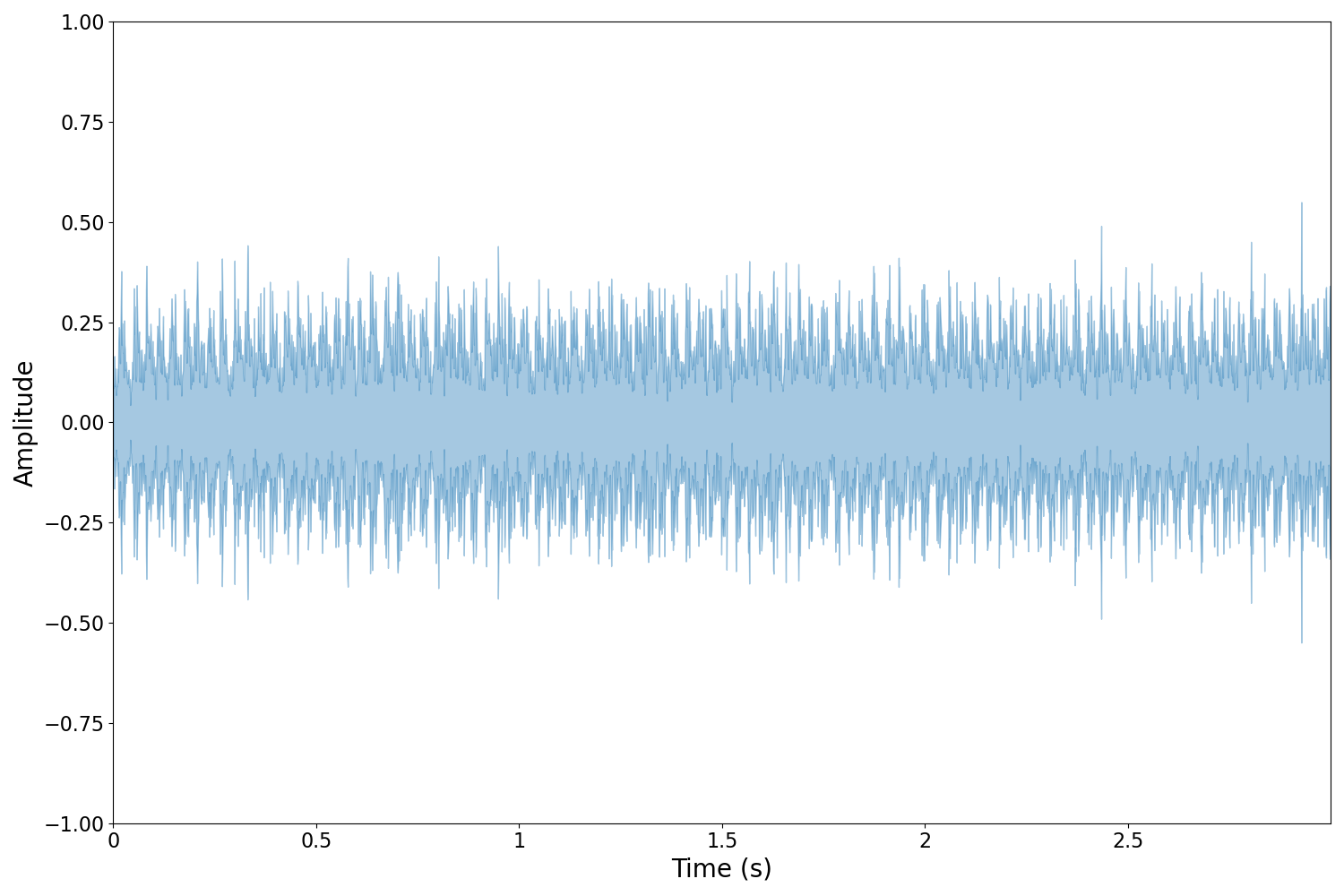
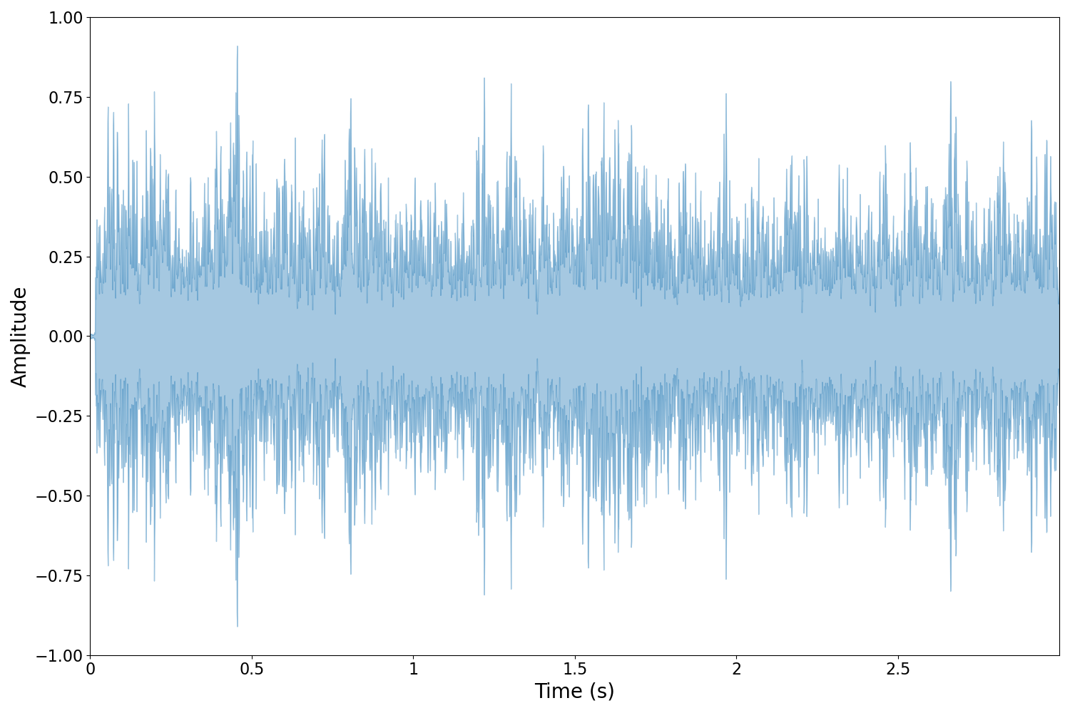
Figure 1: Example of two acoustic vehicle samples as raw waveforms: inline four turbocharged (left) and a V8 with normal aspiration (right). Using the waveform to differentiate between vehicle types is a challenging task.

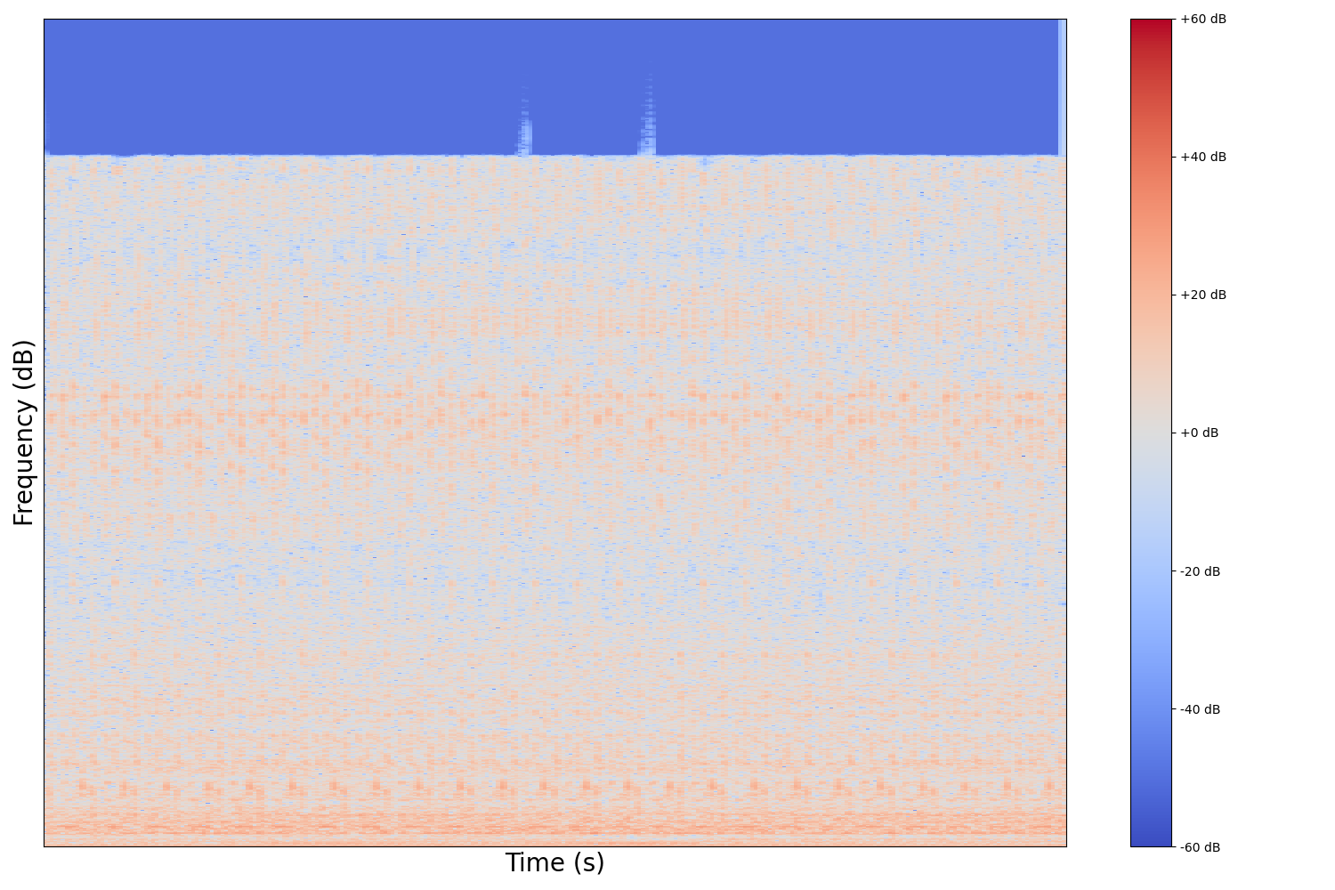
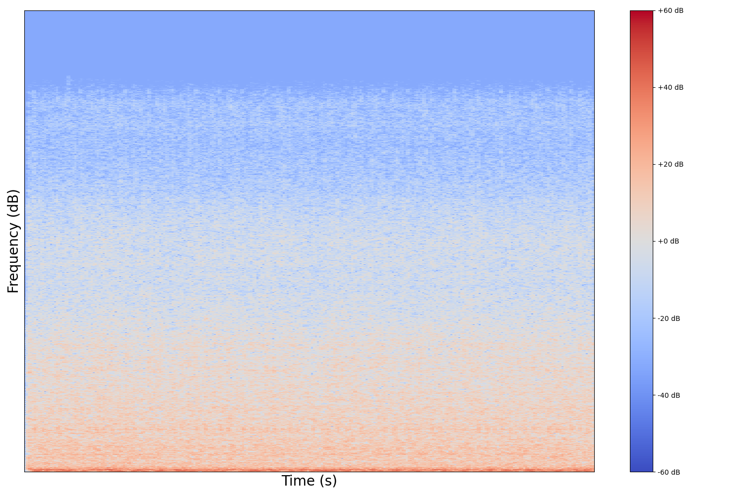
Figure 2: Example of two acoustic vehicle samples as spectrograms: inline four turbocharged (left) and a V8 with normal aspiration (right). Compared to the raw waveform from Figure 1, the spectrogram provides a more informative feature type for vehicle differentiation.

A final challenge in acoustic vehicle understanding is status. In other words, we might ask whether a vehicle is in motion or stationary, or whether a vehicle is performing normally or abnormally. Given that it can take mechanics hours of manual labor and visual inspection to detect complicated issues with vehicles, it is clear how challenging –and subjective –this task may be using only sound data. In this work, we seek to identify whether a vehicle engine is operating normally or misfiring.

To address these challenges and build on the hypothesis that prior knowledge of a system’s configuration can inform appropriate fine-grain classification, we propose novel cascading architectures for vehicle understanding, as visualized in Figure 3. We define a cascading architecture as a multi-level, sequential, conditional network that makes multiple predictions and cascades each prediction to every successive layer of the network. We also compare this architecture to a more conventional multi-task classification approaches. Our representative cascading network has four distinct layers:

1. General acoustic classification: Does the audio sample contain a vehicle?

2. Attribute recognition: What is the kind of vehicle?

3. Status prediction: Is the vehicle performing normally?

4. Fault identification: If abnormal, what fault is occurring?

Our architecture is novel in that it integrates multiple highly-granular classification tasks and also in that the result of each successive classification task might inform the next. Previous work (surveyed in Section 2.2) has shown mastery of both high-level attribute recognition and low-level status prediction, though this article, to the best of our knowledge, is the first to complete these tasks simultaneously in a unified deep neural network network architecture.

In this manuscript, we apply audio data to vehicles as a means of providing enhanced insight towards the goal of reducing vehicle emissions and increasing usable service life. We first motivate the need and value for an automated system of vehicle understanding using sound data and then explore the prior art in sound recognition with deep learning, cascading architectures, acoustic vehicle characterization, and audio data augmentation. We define cascading architectures for vehicle understanding at a high level as multi-level, sequential, conditional networks as visualized in Figure 3.

In a proof-of-concept, we built a two-stage convolutional neural network (CNN) with its first stage specializing in vehicle attributes and then cascading its attribute predictions to the second stage misfire fault detection network. Through this approach, the cascading model achieves $95.6\%$, $93.7\%$, $94.0\%$, and $92.8\%$ validation accuracy on attributes (fuel type, engine configuration, cylinder count, aspiration type, respectively). The cascading CNN also achieved $93.6\%$ misfire fault validation accuracy which was $16.4\%$ and $4.2\%$ better than naïve and parallel baselines, defined as predicting the most probable label and a one-stage multi-task CNN. Although the cascading model does not outperform the parallel baseline across all feature types in outsample test performance, we believe this nascent architecture has the potential to generalize well in real-world vehicle and other system classification scenarios with further refinement, optimization, and access to richer training data.

We provide evidence for the consistency and richness of our model architectures through experimental comparisons across three dimensions: models, features, and tasks. Additionally, we explore ablation studies focused on data augmentation, learning rate, and performance on outsample data captured from YouTube. We conclude with broader implications, future directions, and potential applications for this work.

Figure 3: Flowchart of our proposed cascading architecture for vehicle understanding using audio data. We can see there are four sequential levels with a conditional dependence between levels $1\rightarrow 2$ and $3\rightarrow 4$. Of particular note is the transition between level 2 and 3, as level 2 cascades its attribute predictions to level 3. This work focuses on level 2 and 3 as a proof-of-concept.

2 Prior art

The presented work is novel in several areas:

1. Sound recognition with deep learning

2. Acoustic vehicle characterization

3. Cascading architectures

4. Audio data augmentation

To establish how the present work relates to and builds upon these areas, we now explore prior art in each.

2.1 Sound recognition with deep learning

There is breadth and depth in the history of deep learning [37, 25] for sound-based tasks. One notable and highly recognizable sound-based task is automatic speech recognition (ASR), which looks to transcribe spoken language into written text. Traditional neural networks were first used for ASR [36, 79], later evolving to convolutional neural networks (CNNs) [1, 47] and recurrent neural networks (RNNs) [28, 27], with modern techniques gravitating towards transformers [32, 21, 29, 71]. These differing neural network types have been utilized for diverse and unique sound-based tasks.

One such task that commonly leverages deep learning is general acoustic classification [30]. We define this task as classifying a signal across many labels within broad categories. AudioSet [23], for example, is a popular dataset for general acoustic classification, which contains 527 diverse, hand-annotated classes for 2.1 million YouTube videos. AudioSet [23] provides an ontology for general acoustic classification with seven categories including:

• human sounds (speech, hands, bodily functions)

• animal (domestic, farm, wild)

• music (instrument, genre, mood)

• sounds of things (vehicle, engine, tools, alarms)

• natural (wind, water, storms)

• source-ambiguous

• channel, environment, background

Related prior art focuses on high-level audio classification using neural networks [8, 5, 42, 52, 72, 4, 31, 2]. These works often utilize audio embeddings [3, 17, 35, 24] with transfer learning to better inform the overall acoustic classification task. As observed with the Audioset [23] ontology, there is also a diverse world of sound that extends to low-level fine-grained task prediction. Applications that utilize DL for sound-based tasks range from music genre classification  [33, 45] to medical diagnoses [15, 19, 12] to animal recognition [40, 64, 74, 82, 80, 11] and more [39, 67, 38].

We build on similar classification techniques and differentiate our work in two ways: first, we focus on multiple low-level, fine-grained multi-level label prediction with the assumption of the highest-level class, rather than simply classifying a single level at a time. Given our approach focuses on these fine-grained tasks, we do not utilize general acoustic embeddings [3, 35, 24] but rather train lightweight models from scratch.

Second, we utilize data collected at a higher sampling rate ($48$ kHz) compared to that collected from YouTube, which we show Section 5.3 caps its sampling rate and in the process may discard useful informative features. This is important because models trained on such crowd-sourced audio may not perform as well as models trained and operated using raw, full-frequency audio directly collected from a mobile device. YouTube and other such sources also conduct feature-destructive compression on some audio samples, which can limit model performance and generalizability.

In summary, our approach uses larger frequency ranges to provide detailed classification lower into the stack, building on techniques demonstrated by prior art.

2.2 Acoustic Vehicle Characterization

Our work is novel in its application of sound-based deep learning, as we focus on acoustic vehicle characterization. Prior art [58] has conducted an extensive survey on off-board vehicle vibro-acoustic diagnostics which explores a multitude of acceleration- and sound-based vehicle characterization approaches. Our work focuses on the lesser-explored tasks of vehicle attribute recognition, engine misfire fault detection, and specifically the interrelation between vehicle variant and fault-specific diagnostic algorithms.

Previous work has focused on vehicle attribute recognition [16, 58] utilizing traditional ML techniques such as SVMs and feature selection. These primarily consider the FFT and MFCC feature types, whereas our work considers five distinct feature types and conducts an in-depth feature comparison. These works also do not consider the engine configuration attribute task. Our work explores the three previously explored attribute prediction tasks: fuel type, cylinder count, aspiration type, as well as the engine configuration task. [16, 58] also build separate models for each prediction task, whereas our deep learning approach demonstrates that predicting attributes jointly in a single model can yield strong results, with variant-identifying parameters helping to “shape” the final diagnostic model.

One research study looking to identify specific faults [59] collects nearly $1k$ audio samples of vehicles using smartphone microphones for which approximately $1/3$ are abnormal “vehicle misfire” events. Using traditional machine learning techniques and various audio features combined with feature selection, [59] achieves $1.0\%$ misclassification rate and $1.6\%$ false positive rate. However, this previous work was trained on three vehicles types and it is unclear if and how the results would generalize to a broader sample including more diverse vehicles.

Our work is unique in its merging of vehicle acoustic characterization tasks. First, classifying attributes for an abnormally performing vehicle may be a more challenging task and [16, 58] only focused on normally performing vehicles. Second, we show the value of multi-task learning through attributes prediction improving misfire performance and vice versa. Finally, we demonstrate a proof-of-concept for a cascading architecture by with our two-stage CNN which uses the first stage to specialize on attributes and then cascade its attribute predictions to the second stage misfire detection network.

2.3 Cascading architectures

We envision our cascading architecture for vehicle understanding as a sequential, conditional model. Specifically, we construct an architecture with four sequential levels (Figure 3), where levels $1\rightarrow 2$ and $3\rightarrow 4$ are conditionally dependent. Additionally, level 3 is dependent upon the cascaded result from level 2.

There is valuable related work in sequential and conditional deep learning that has been utilized in a select applications. Examples include human activity recognition [78], image segmentation [70], facial recognition [75], frame prediction in games [69], and music rhythm generation [41].

There are three works of particular relevance to our cascading architecture for acoustic vehicle characterization:

• An Ontology-Aware Framework for Audio Event Classification [65]

• Masked Conditional Neural Networks for sound classification [43]

• CascadeML: An Automatic Neural Network Architecture Evolution and Training Algorithm for Multi-label Classification [46]

We now discuss how our work differs from these approaches.

[65] has elements that are similar to our proposed cascading architecture. Specifically, [65] leverages the relationship between fine and coarse labels in their model training. The first and second level of our cascading architecture can be seen as examples of coarse and fine labels, which have a subset relationship. However, [65] does not consider conditional logic and does not have multiple levels like our proposed cascading architecture.

Both [43] and our work utilize neural networks for acoustic classification. However, the conditional component of [43] does not correspond with multi-label dependence proposed in our cascading architecture but rather conditional dependence in the data itself. Specifically, [43] leverages the temporal relationship of nearby frames in spectrograms whereas our work utilizes the entire spectrogram, agnostic to its temporal nature, as a feature set in the CNN.

CascadeML [46] is closely related to our proposed architecture. Our architecture might almost be considered an example of the theoretic structure proposed by [46]. However, [46] focuses on the AutoML component where the network can dynamically grow itself based upon any number of multi-label samples. We instead embed expert knowledge into the static structure of the cascading architecture. In other words, we know fault type is conditional upon status prediction, so we embed that in the structure of our architecture rather than building a network from scratch with the AutoML approach of [46]. Not only will this approach allow us to demonstrate stronger and more consistent performance, but also it would be theoretically more efficient given it structure is already defined.

In summary, [65, 43, 46] showcase various sequential, conditional, and cascading architectures that are closely related to our work. However, these works focus on either theoretical or high level acoustic classification. We show there is value in building a model for the specific application of acoustic vehicle characterization.

2.4 Audio Data Augmentation

In deep learning for computer vision, there is value applying data augmentation to images via rotations, cropping, scaling, etc. to gain invariance among unique inputs. Audio may similarly be augmented. [50] utilized time stretching, dynamic range compression, pitch shifting, and background noise for environmental sound classification. In speech recognition, [34] applied multiple speed changes to expand their training set. Focused on animal audio classification, [44] uniquely applies computer vision augmentation techniques to the spectrogram such as reflection and rotation, as well as waveform augmentation with pitch, speed, volume, random noise, and time shift. For music classification, [51] found pitch-shifting to be most informative but also utilizes time stretching and random frequency filtering.

There is prior art involving data augmentation for acoustic vehicle characterization. Researchers [77] classify accelerating vehicles using audio and apply random noise and pitch shift to expand their dataset. Other work [14] focuses on vehicle type identification using MFCCs and other audio features, these authors apply city noise to augment captured signals. There have been additional applications of augmentation to acoustic vehicle DL related tasks [7, 13, 53].

Our work is similar to [51, 50, 44] in that we utilize pitch, speed, volume, and random noise augmentation types. However, we differentiate ourselves in our application of the augmentation to multi-task learning for vehicle attribute recognition and fault detection. Additionally, to our knowledge, our approach is unique in that our train set is not a combination of real and augmented samples but is entirely made up of augmented samples. We hypothesize this may allow for more robust training and less overfitting / memorizing of specific samples. We also show in Section 5.1 the strong, positive impact augmentation has on our model performance.

3 Approach

As noted in the problem motivation, proper maintenance is increasingly important to vehicles as their number and miles travelled grow. However, as vehicles become more like appliances and less familiar to their users, driver and passenger awareness of their capabilities diminishes. We suggest that automated vehicle identification is an important first step in diagnosing and rectifying problems plaguing efficiency and emissions: when a part fails, it is not enough to know that a vehicle is big or small, or red or silver, but rather that a vehicle is a 2016 version of some specific make and model possessing a particular engine and transmission type and tire size. Creating tools that effectively identify vehicles and use these attributes as a means of improving state characterization allows non-expert users to expertly diagnose their own vehicles, clearing the knowledge hurdle to effective maintenance and thereby reducing fuel consumption, emissions, and likelihood of breakdown.

Our approach is a proof-of-concept for how vehicle characteristics can better inform fault diagnoses and in this section we explain our approach from five main angles:

1. Datasets

2. Features

3. Model

4. Network

5. Implementation

First, we share the details of our novel dataset, specifying the dataset splits and augmentation procedure. Second, we compare the different audio feature types used in our models. Third, we develop a high-level understanding of the two multi-task models proposed in this work. Then, we clarify the specifics of the CNNs for each main feature type. Finally, we provide implementation details to aid in reproducibility.

3.1 Datasets

Our dataset is a collection of audio samples recorded using mobile phones. We utilize mobile phone microphones as these tend to have repeatable characteristics within the range of frequency similar to those of human speech and hearing (roughly $20$Hz-$20$kHz). In particular, we merge the datasets from [16, 58], which focus on attributes, with [59, 56], which focus on misfire detection. We outline the makeup of our dataset and its splits in Table 1.

Table 1: Summary of the train/validation/test split for our datasets. We create 8 augmented training samples per one validation sample. The test sets is mutually exclusive from the train and validation sets, which allows it to provide an insight into the outsample performance and model generalizability.

Dataset Split	Raw Samples	Clips (3 sec)	Total Length (min)
Train	–	43640	2182.0
Validation	228	5455	272.75
Test	58	951	47.55
Total	286	50046	2502.3

Together, these datasets totaled $286$ ($228+58$) audio samples, which contributed to about 320 minutes of non-augmented audio. We decided to split each audio sample into three second clips (“chunks”) to provide our features and models with a standard input size for training and to expand our dataset size. This time was selected as striking an appropriate balance of capturing low-frequency sounds with ease and speed of capture. Additionally, we believe three seconds is a long enough sample to be representative data for our model, but also short enough that would allow for clips within the same sample to be distinct and useful for training. After chunking the samples, this resulted in $6406$ ($5455+951$) unique three second clips. Though fixed-length clips were used, our models at test time are agnostic to the input feature size, rather than needing the sample to be exactly three seconds.

Our approach for the train/validation/test split involved building a train set using only augmented clips with the goal of reducing overfitting and improving generalizability. In turn, we split the real full length samples into a validation and test set, using a traditional 80/20 split. As seen in Table 1, this resulted in $5455$ validation clips and $951$ test clips. We split the validation and test set using the raw samples rather then the clips because we created the train set using only the validation set. This allowed for the test set to be mutually exclusive from both the train and validation set to showcase as accurate as possible the model’s outsample generalizability.

Due to the relatively small size of the datasets, we manually created the validation and test splits with an attempt to balance the label distribution to the best of our ability for the four attribute recognition tasks: fuel type, engine configuration, cylinder count, and aspiration type and the status prediction task focused on misfire detection. Label distributions are visualized in Figures 4 and 5.

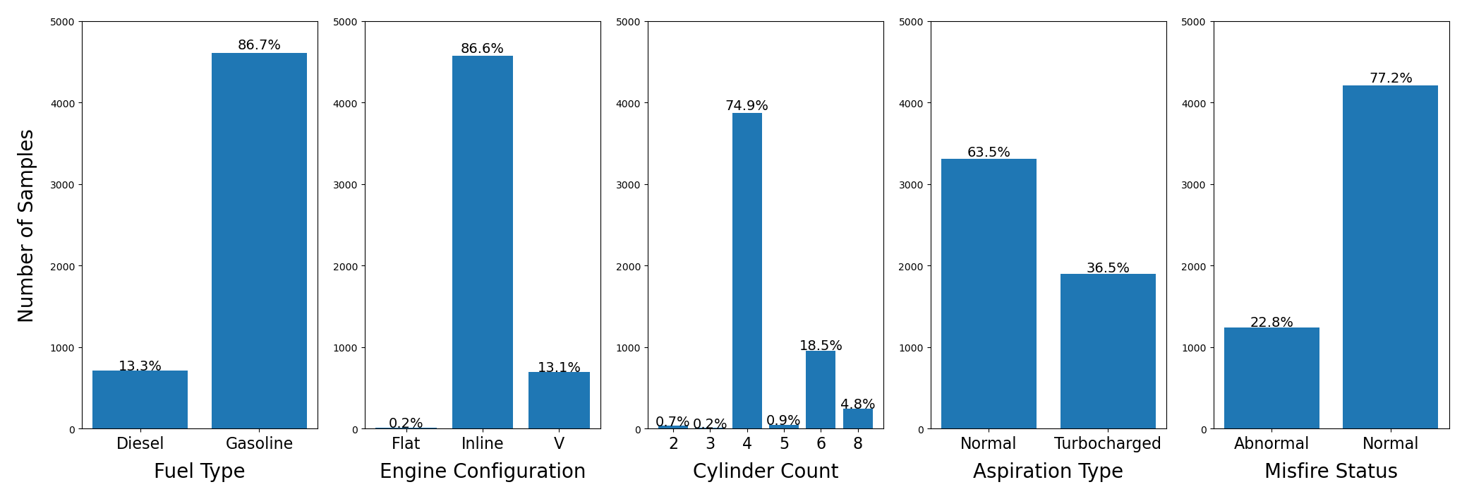
Figure 4: Label distribution for the validation set. We observe the classes are not perfectly balanced and some labels in the engine configuration and cylinder count are very underrepresented.

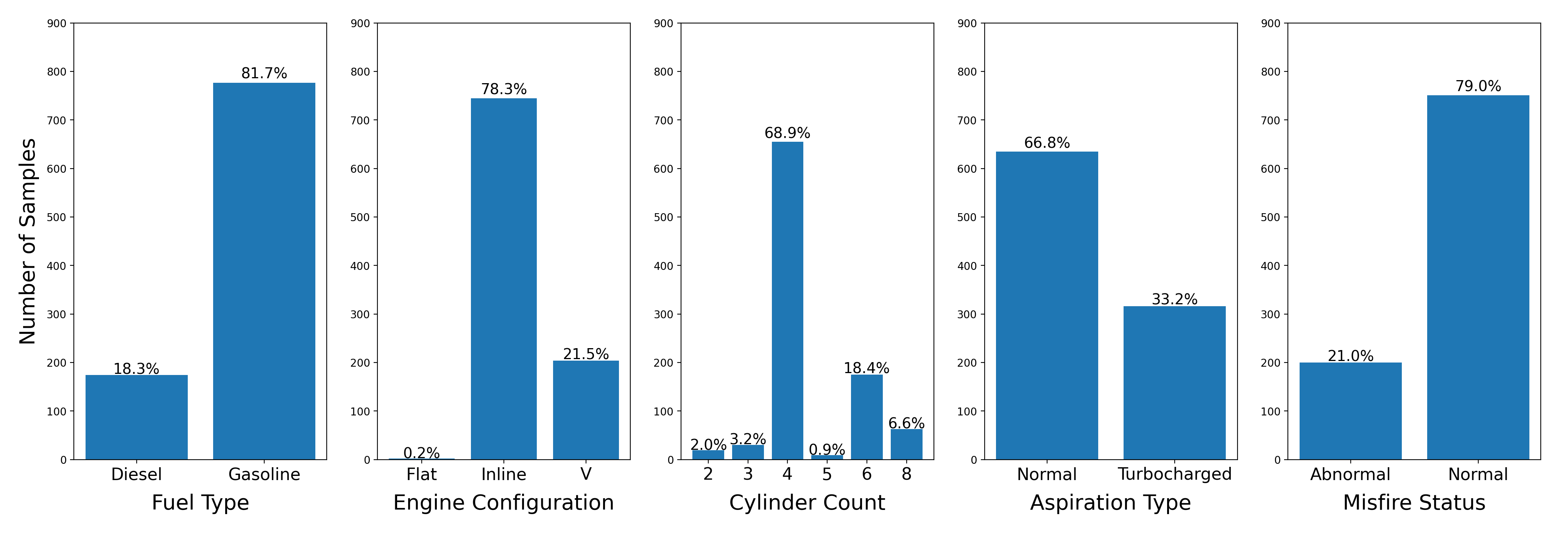
Figure 5: Label distribution for the test set. We attempted to build a test set with as similar label distribution to training and validation as possible, while also including at least one raw sample from each label.

Our process of creating the training set consisted of applying a data augmentation process eight times to each of the $5455$ validation clips, which when expanded resulted in a train set of size $43640$ as seen in Table 1. The data augmentation process consisted of applying four types of data augmentation to each clips which each data augmentation type having a probability of $50\%$ of being activated. The types of augmentation chosen were volume change, pitch shift, speed shift, and random background noise. More specifically, we chose each type of augmentation from a randomly uniformly distribution over these augmentation parameters:

• Change volume between -5.0 and 5.0

• Pitch shift between -0.25 and 0.25

• Change speed between 0.92 and 1.08

• Add background noise with signal to noise ratio (SNR) between 0.05 and 0.20.

We also add epsilon between $10^{-6}$ and $10^{-5}$ to each parameter, so as to not randomly choose a hyperparameter of zero volume change / pitch shift or one for speed change, which would result in the clip not being augmented at all. Additionally, if the clip was not changed after all four augmentation types rolled their probability (i.e. all four types were not activated), we applied one augmentation type at random. This guaranteed that no training clips were exactly the same as their respective validation clip. All value ranges were determined experimentally, with expert mechanic review to coarsely validate the “closeness” of the augmented sample with the original sample. Augmentation parameters were set so as to line up with typical variation in engine configurations, e.g. through manufacturing diversity and wear. For example, frequency shift was bounded based on typical allowable tolerances for idle speed. Amplitude limits were set so as to minimize the effect of signal clipping. The features were determined to be acoustically-discernible after augmentation.

We further motivate our decision for using data augmentation later in Section 5.1.

In summary, we created a new dataset with a non-traditional train/validation/test split. This set uses only augmented variants of validation samples in training and is mutually exclusive from both the validation and test set. Our dataset, per Table 1, in total consisted of $50046$ three second clips for a total of $2502.3$ minutes or about $42$ hours total of audio.

3.2 Features

In this work, we explore four audio feature types (five when considering the raw waveform) which include:

• Fast Fourier Transform (FFT)

• Mel-frequency Cepstral Coefficients (MFCCs)

• Spectrograms

• Wavelets

Examples of these feature types can be visualized in Figures 1-2 and 6-8.

These features were chosen to give our models a diverse set of inputs. The raw waveform provides the model with time information, while the FFT provides the model with frequency information. MFCCs, Spectrograms, and Wavelets provide the model with varying degrees of hybrid time and frequency information at different dimensionality.

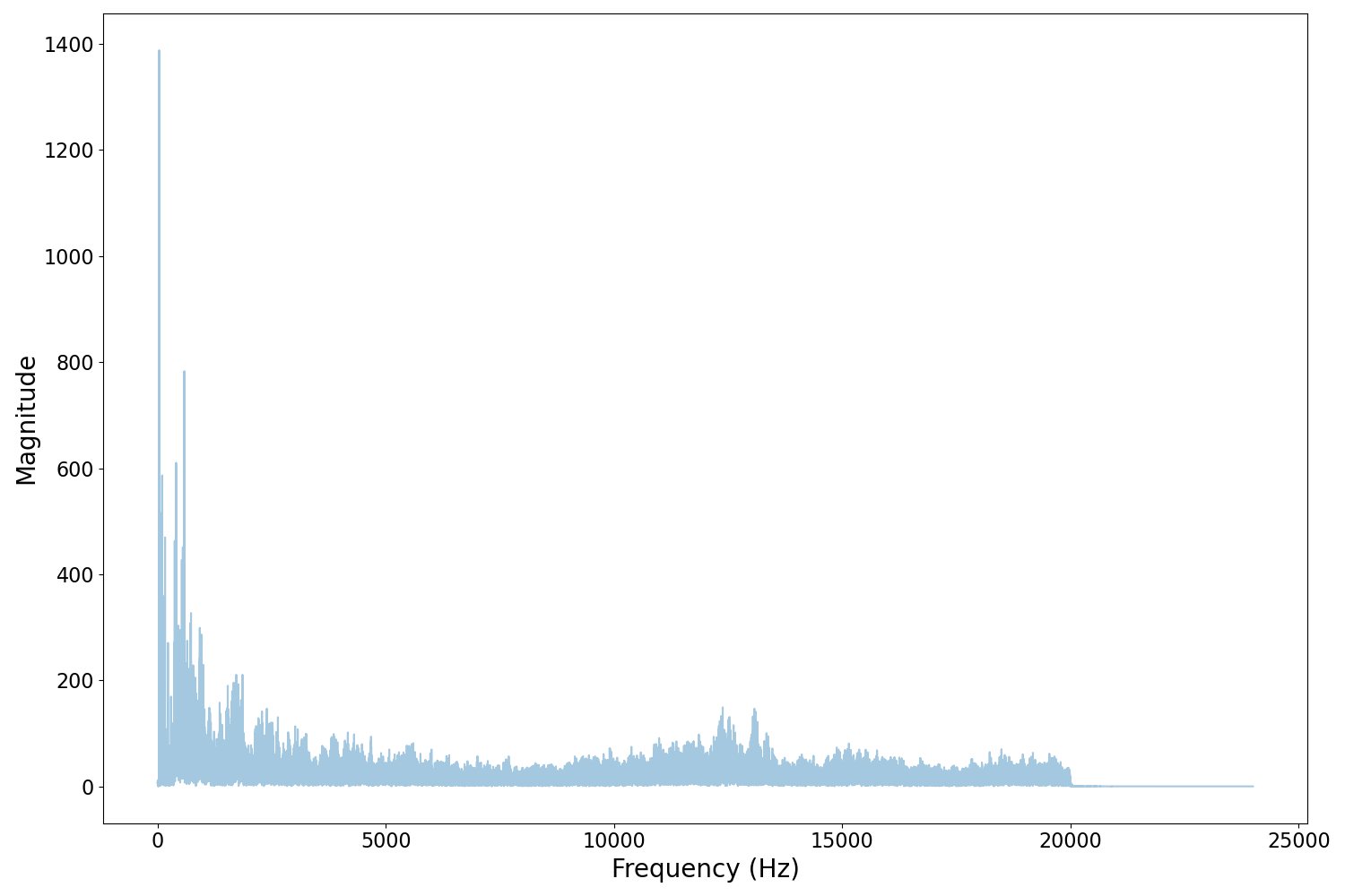
Figure 6: Example of FFT audio features, which are binned by frequency (24,000 bins which correspond to the 24kHz sampling rate and represented with a long 1D vector.

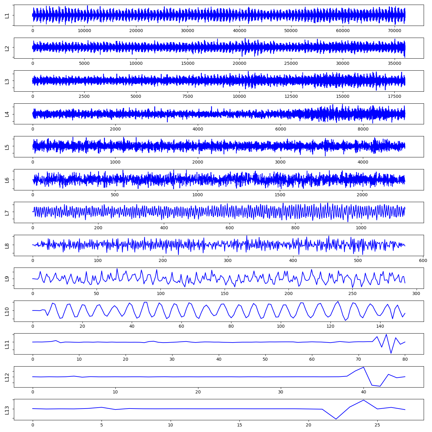
Figure 7: Example of wavelet audio features, which use to 13 levels of decomposition and then are stacked horizontally to create one long 1D vector.

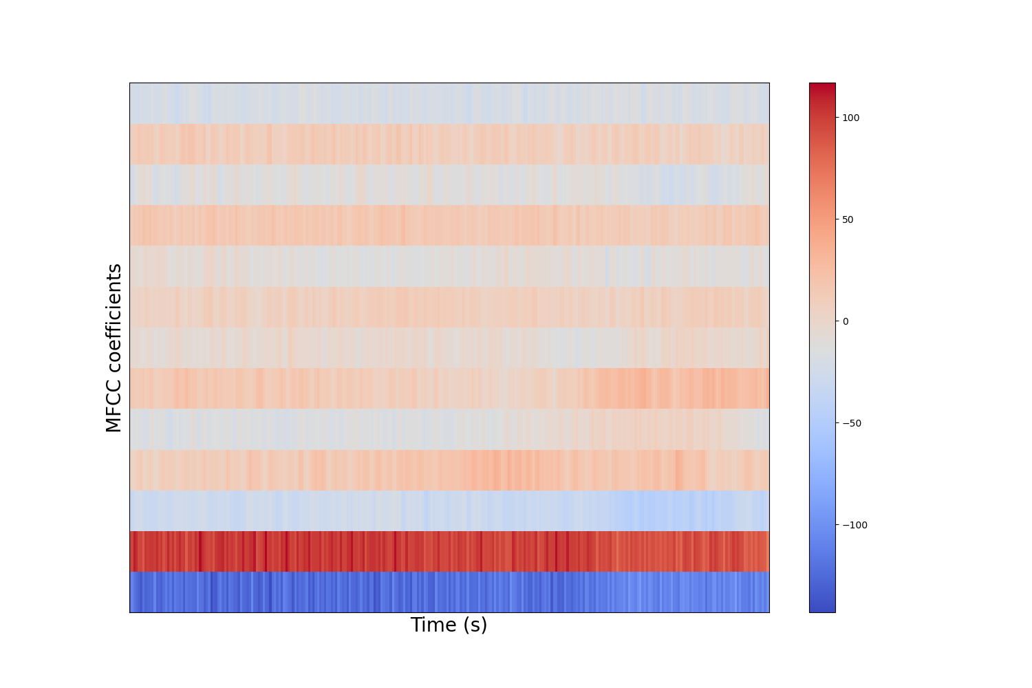
Figure 8: Example of MFCC audio features for which 13 coefficients were chosen as a hyperparameter. MFCC features are later shown to be the more impactful in our deep learning models.

3.3 Model

We design and implement a variant of the earlier-proposed Cascade model: a two-stage network for which the first stage specializes on attributes classification and the second stage specializes on misfire detection. The first stage receives one of the previously described feature sets as input. The second stage receives both the feature set and the attribute predictions from the first stage. Both stages are trained jointly using multi-task learning.

To compare against the Cascade model, we also consider two baselines: Naïve and Parallel models. The Naïve model is a straightforward baseline that predicts the most represented class for each task. For example, if we look at Figure 4, the Naïve model would always predict gasoline as the fuel type. This model would achieve $86.7\%$ validation accuracy.

The Parallel model, as seen in Figure 9, represents a more complex baseline to consider than the Naïve model. The Parallel model is represented as a sequential, multi-level, conditional network in the same archetype as the Cascade model. However, per Figure 9, it does not explicitly cascade, or provide as input, the classified vehicle type to the status prediction level. Rather, these two tasks are predicted in parallel from the raw waveform and/or features.

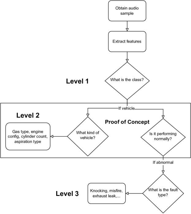
Figure 9: Flowchart of our baseline Parallel model architecture. The Parallel model is differentiated from the Cascade model in that rather than level 2 cascading to level 3, we combine these levels in parallel.

Both the Cascade and Parallel model are viable classification approaches: both serve as a proof-of-concept for a full scale AI mechanic architecture and provide an all-in-one solution for classifying attributes and misfire. The Cascade and Parallel models also both utilize multi-task learning to allow for the attributes prediction to better inform the misfire prediction and vice versa. However, the models differ in their internal sharing of intermediate classification representations. Therefore, there is value in the comparison on whether a joint, shared representation via the Parallel model or separate, specialized representations via the Cascade model would yield better performance. It is also worth noting that given the Cascade model has a second sequential stage, there is an non-negligible increase in model runtime and memory. In turn, these factors should be worth considering if the Cascade model provides a margin on any task predictions.

These two models are directly compared in Figure 10.

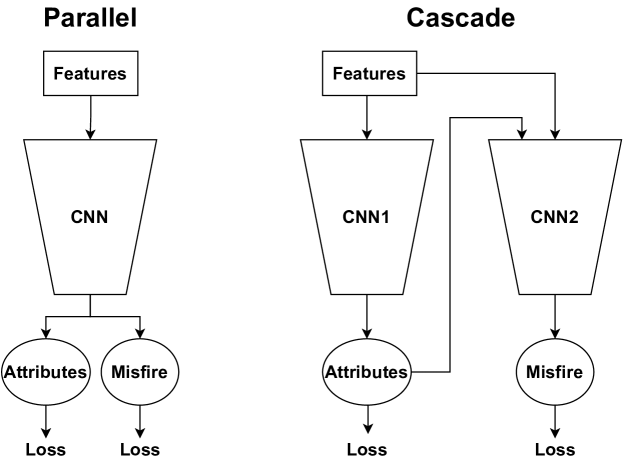
Figure 10: Parallel and Cascade CNN model architecture comparison. We observe the Parallel model uses a shared representation for both the attributes and misfire predictions whereas the Cascade model has two distinct CNNs that allow for specialization in attributes and misfire. Additionally, both networks utilize multi-task learning so the attributes loss can inform the misfire loss and vice versa.

3.4 Network

We propose two distinct multi-layer convolutional neural networks (CNNs), Parallel and Cascade, to predict both vehicle attributes and engine misfire, as seen in Figure 10.

For each, we group audio features into 1D (FFT, waveform, wavelets) and 2D (Spectrogram, MFCCs) sets, with two two distinct model architectures that utilize 1D and 2D convolution respectively. We adapt the M5 architecture [18] which was built for general audio classification using the raw waveform.

Our samples utilize a $48$ kHz sampling rate, for which we consider frequencies $\leq 24$ kHz according to the Nyquist-Shannon Sampling Theorem. These samples were collected using a stereo microphone for which we average the dual channel input into a single mono channel. We split each sample into 3 second chunks which results in a $1\times 72,000$ input vector for the raw waveform.

The unique aspect of the M5 model utilizes a large convolutional kernel size of $80$ in the first layer to propagate a large receptive field through the network. We adopt kernel size of $3$ from [18] for the remaining three convolutional layers.

For the MFCC model we utilize kernel size of $2\times 2$ since we chose $13$ MFCC coefficients as a hyperparameter which results in an input dimensionality of $130\times 13$. For the spectrogram, we choose hyperparameters of $512$ for hop length and $2048$ for window size. This results in a input dimensionality of $1025\times 282$. Since it was a larger input dimension than the MFCCs, we utilize traditional $3\times 3$ kernels for spectrogram.

For the 2D models, our model consists of three convolution layers, rather than four layers for the 1D models because of their smaller input width. We follow the precedent set by [18] for including pooling, batchnorm, and ReLU after each conv layer in both 1D and 2D models. We also add dropout with probability $=0.5$ after each layer to improve generalizability and to minimize the likelihood of overfitting. We treat each prediction task as classification and therefore have final fully connected output layers with dimensionality corresponding to the number of classes for each task. These predictions are then fed into log softmax and trained using negative log-likelihood loss.

3.5 Implementation

We built our models using PyTorch within an Anaconda environment. We trained our models using 1080 Ti and Titan XP GPUs. Our models unless otherwise stated were trained for $100$ epochs with the Adam optimizer, utilizing a batch size of $128$, learning rate of $0.001$, no weight decay, and with amsgrad following the standard set by [18] for training CNNs on audio. The Spectrogram model did not fit into GPU memory with a batch size of $128$, so a batch size of $64$ and $32$ were used for the Parallel and Cascade models, respectively.

We conducted a handful of hyperparameter searches to find the best set for each model type, across number of epochs, learning rate, and dropout rate. Specifically, we looked at number of epochs ranging from $10$ to $100$, learning rate ranging from $0.0001$ to $0.1$, and dropout rate ranging from $0.0$ to $0.75$. These experiments did not yield any notable trend and in turn have not included these results in our manuscript. However, any model weights and log files are available via request for reproduciblility. For the following Sections 4 and 5, we utilize the hyperparameters which result in the top performing model for each feature type.

Our dataset and code are undergoing an IP review and are expected to be released to the public.

4 Results

We evaluate classifier performance along three dimensions:

1. Model Comparison

2. Feature Comparison

3. Task Comparison

For model comparison, we first compare our Parallel and Cascade architectures as seen in Figure 10. Our goal is to provide unbiased data and to learn the scenarios under which each model performs better or worse than the other. We hypothesize that the Cascade model will demonstrate better performance on the misfire fault detection task over the Parallel approach. Next, with the feature comparison subsection, we illustrate the impact the choice of audio feature has on model accuracy. Finally, we delve into task comparison to better understand how our top performing models are classifying each of the four main attributes: fuel type, engine configuration, cylinder count, and aspiration type, as well these labels’ contribution to misfire fault detection performance. We include evaluation metrics (precision/recall) and confusion matrices to provide additional insight into the true value of our approaches.

4.1 Model Comparison

Table 2 compares the validation set accuracy for each feature type between the Naïve, Parallel and Cascade models. We first note that both the Parallel and Cascade models significantly outperform the Naïve model in both attribute and misfire prediction. Next we find that the Cascade model demonstrate minor improvements or degradation over the Cascade model for attributes across our feature types. Finally, the Cascade model outperforms the Parallel model across every feature type for misfire prediction. Specifically, we observe 7.4%, 4.2%, 0.7%, 12.3%, 2.7% validation set accuracy improvements for FFT, MFCC, spectrogram, waveform, and wavelet model performance respectively.

In exploring the test set results in Table 3, we observe similar patterns. With respect to the Naïve baseline, it appears that the Parallel and Cascade models plateau for attributes. However, for misfire prediction the Cascade model outperforms both the Naïve and Parallel baselines across every feature type. Specifically, when comparing Parallel and Cascade model test set accuracy on the misfire task, we observe 4.0%, 1.5%, 1.0%, 8.8%, 1.7% improvements for FFT, MFCC, spectrogram, waveform, and wavelet model performance respectively.

The major takeaway: the Cascade model outperforms all baselines on misfire prediction. These findings show we have achieved our goal of improving fault prediction through cascading of vehicle attributes..

Table 2: Model comparison for validation set accuracy. We observe for the four attribute prediction tasks, Parallel and Cascade achieve similar performance whereas for the misfire task Cascade outperforms Parallel across all feature types.

Model	Feature	Fuel	Config	Cyl	Turbo	Misfire
Naïve	–	86.7%	86.6%	74.9%	63.5%	77.2%
Parallel	FFT	90.1%	89.9%	78.2%	80.0%	84.4%
Cascade	FFT	90.4%	89.9%	81.4%	77.5%	91.8%
Parallel	MFCC	96.0%	94.0%	93.6%	92.9%	89.4%
Cascade	MFCC	95.6%	93.7%	94.0%	92.8%	93.6%
Parallel	Spectrogram	87.7%	86.7%	75.9%	80.0%	85.8%
Cascade	Spectrogram	87.4%	86.6%	76.2%	78.4%	86.5%
Parallel	Waveform	95.2%	93.5%	90.1%	90.5%	81.1%
Cascade	Waveform	94.9%	92.0%	90.8%	92.0%	93.4%
Parallel	Wavelets	85.9%	69.2%	59.5%	80.5%	86.7%
Cascade	Wavelets	86.6%	76.4%	67.9%	81.4%	89.4%

Table 3: Model comparison for test set accuracy. We again observe relatively similar performance across attributes between Parallel and Cascade, while the Cascade model consistently improves upon the Parallel model for misfire prediction.

Model	Feature	Fuel	Config	Cyl	Turbo	Misfire
Naïve	–	81.7%	78.3%	68.9%	66.8%	79.0%
Parallel	FFT	78.8%	78.3%	67.7%	70.6%	79.5%
Cascade	FFT	81.7%	77.8%	68.1%	66.5%	83.5%
Parallel	MFCC	84.7%	78.3%	72.0%	73.0%	85.3%
Cascade	MFCC	81.6%	78.2%	67.3%	70.1%	86.8%
Parallel	Spectrogram	77.0%	78.3%	68.9%	65.9%	84.9%
Cascade	Spectrogram	81.7%	78.3%	68.9%	67.2%	85.9%
Parallel	Waveform	73.3%	75.2%	64.7%	67.7%	70.8%
Cascade	Waveform	82.0%	78.3%	52.5%	67.3%	79.6%
Parallel	Wavelets	79.9%	63.4%	52.7%	69.0%	81.4%
Cascade	Wavelets	78.4%	62.1%	53.1%	66.8%	83.1%

4.2 Feature Comparison

We explore model performance for five feature types (FFT, MFCC, spectrogram, wavelets, waveform). FFT, wavelets, and waveform share the exact same model architecture, whereas MFCC and spectrogram each use a unique model architecture with differing amounts of layers and kernel sizes to reflect the feature dimensionality.

In investigating validation set performance from Table 4, we see that MFCC features outperform all other feature types in both the Parallel and Cascade models. When exploring the test set performance from Table 5, we again find MFCC is again the top performing feature for the Parallel and Cascade models. We also note that the models with spectrogram features achieve second place for both Parallel and Cascade on the test set. This shows that the models which utilize 2D convolution are able to find more generalizable patterns from the train set to the test set. The final pattern we can observe is the poor performance of the raw waveform relative to the other feature types. This demonstrates the value of our experiments which analyze many different types of audio features.

Table 4: Feature comparison for validation set accuracy. MFCC features perform the strongest across all attributes and misfire for both the Parallel and Cascade models.

Model	Feature	Fuel	Config	Cyl	Turbo	Misfire
Parallel	MFCC	96.0%	94.0%	93.6%	92.9%	89.4%
Parallel	Wavelets	85.9%	69.2%	59.5%	80.5%	86.7%
Parallel	Spectrogram	87.7%	86.7%	75.9%	80.0%	85.8%
Parallel	FFT	90.1%	89.9%	78.2%	80.0%	84.4%
Parallel	Waveform	95.2%	93.5%	90.1%	90.5%	81.1%
Cascade	MFCC	95.6%	93.7%	94.0%	92.8%	93.6%
Cascade	Waveform	94.9%	92.0%	90.8%	92.0%	93.4%
Cascade	FFT	90.4%	89.9%	81.4%	77.5%	91.8%
Cascade	Wavelets	86.6%	76.4%	67.9%	81.4%	89.4%
Cascade	Spectrogram	87.4%	86.6%	76.2%	78.4%	86.5%

Table 5: Feature comparison for test set accuracy. For the Parallel model MFCC features translate their strong validation performance to test set generalizability. However, the Cascade model better utilizes FFT and spectrogram features for attributes and spectrogram and wavelet features for misfire.

Model	Feature	Fuel	Config	Cyl	Turbo	Misfire
Parallel	MFCC	84.7%	78.3%	72.0%	73.0%	85.3%
Parallel	Spectrogram	77.0%	78.3%	68.9%	65.9%	84.9%
Parallel	Wavelets	79.9%	63.4%	52.7%	69.0%	81.4%
Parallel	FFT	78.8%	78.3%	67.7%	70.6%	79.5%
Parallel	Waveform	73.3%	75.2%	64.7%	67.7%	70.8%
Cascade	MFCC	81.6%	78.2%	67.3%	70.1%	86.8%
Cascade	Spectrogram	81.7%	78.3%	68.9%	67.2%	85.9%
Cascade	FFT	81.7%	77.8%	68.1%	66.5%	83.5%
Cascade	Wavelets	78.4%	62.1%	53.1%	66.8%	83.1%
Cascade	Waveform	82.0%	78.3%	52.5%	67.3%	79.6%

4.3 Task Comparison

We explore the confusion matrices for each of the four attribute and the misfire prediction tasks:

1. Fuel Type

2. Engine Configuration

3. Cylinder Count

4. Aspiration Type

5. Misfire Detection

These results use both the Parallel and Cascade Models with the top performing feature type, MFCCs.

4.3.1 Fuel Type

With our first prediction task, fuel type, in Table 7 we observe very high validation set accuracy ($98\%$) on the gasoline class. However, due to class imbalance, the Diesel class validation accuracy was lower ($84\%$). This pattern follows in Table 8 with strong test set accuracy on gasoline ($97\%$). Unfortunately, there was a significant degradation from validation to test set accuracy on the underrepresented Diesel class ($32\%$). This is further represented in the precision and recall metrics in Table 6 with Cascade achieving 90.4% precision and 89.1% recall on the validation set while degrading to 63.5% precision and 67.6% recall on the test set.

Of note, the Cascade model outperformed the Parallel model on the underrepresented Diesel class in both validation and test sets. We hypothesize the Cascade model is able to perform better on the underrepresented class due to its separate stage CNNs, allowing the network more distinctly differentiate samples, particularly those that are abnormal and may be more difficult to classify.

Table 6: Fuel Type validation and test set metrics using MFCC features.

Model	Set	Accuracy	Precision	Recall
Parallel	Validation	96.0%	88.1%	90.4%
Cascade	Validation	95.6%	90.4%	89.1%
Parallel	Test	84.7%	60.5%	66.5%
Cascade	Test	81.6%	63.5%	67.6%

Table 7: Fuel Type validation confusion matrix for Parallel (left) and Cascade (right) using MFCC features.

		Predicted
		Diesel	Gasoline
Actual	Diesel	580 (81.8%)	129 (18.2%)
	Gasoline	83 (1.8%)	4525 (98.2%)

		Predicted
		Diesel	Gasoline
Actual	Diesel	594 (83.8%)	115 (16.2%)
	Gasoline	142 (3.1%)	4466 (96.9%)

Table 8: Fuel Type test confusion matrix for Parallel (left) and Cascade (right) using MFCC features.

		Predicted
		Diesel	Gasoline
Actual	Diesel	43 (24.7%)	131 (75.3%)
	Gasoline	22 (2.8%)	755 (97.1%)

		Predicted
		Diesel	Gasoline
Actual	Diesel	56 (32.2%)	118 (67.8%)
	Gasoline	58 (7.5%)	719 (92.5%)

4.3.2 Engine Configuration

Our next prediction task focused on engine configuration: Flat (Boxer), Inline, or Vee. Validation and test set results are seen in Table 10 and Table 11, respectively. The first observation is the lack of representation with the rare engine configuration class of Flat, which therefore did not lead to the identification of a meaningful informative feature pattern.

Similarly to Fuel Type, our models show strong performance on the most well-represented class, in this case, Inline with $98\%$ and $93\%$ validation and test set accuracy respectively. The secondary class V configuration achieves underwhelming validation accuracy of $67\%$ with again degradation down to $26\%$ on the test set. Further elucidated in Table 9 where the Cascade model precision and recall degrades from 73.2% and 79.9% to 49.8% and 53.7% from validation to test set.

Table 9: Engine Configuration validation and test set metrics using MFCC features.

Model	Set	Accuracy	Precision	Recall
Parallel	Validation	94.0%	73.5%	79.6%
Cascade	Validation	93.7%	73.2%	79.9%
Parallel	Test	78.3%	47.2%	49.6%
Cascade	Test	78.2%	49.8%	53.7%

Table 10: Engine configuration validation confusion matrix for Parallel (top) and Cascade (bottom) using MFCC features.

		Predicted
		Flat	Inline	V
Actual	Flat	0 (0.0%)	7 (53.9%)	6 (46.1%)
	Inline	0 (0.0%)	4499 (98.4%)	73 (1.6%)
	V	0 (0.0%)	229 (33.0%)	464 (67.0%)

		Predicted
		Flat	Inline	V
Actual	Flat	0 (0.0%)	7 (53.9%)	6 (46.1%)
	Inline	0 (0.0%)	4474(97.9%)	98 (2.1%)
	V	0 (0.0%)	250 (36.1%)	443 (63.9%)

Table 11: Engine Configuration test confusion matrix for Parallel (left) and Cascade (right) using MFCC features.

		Predicted
		Flat	Inline	V
Actual	Flat	0 (0.0%)	0 (0.0%)	2 (100.0%)
	Inline	0 (0.0%)	696 (93.4%)	49 (6.6%)
	V	0 (0.0%)	154 (75.5%)	50 (25.5%)

		Predicted
		Flat	Inline	V
Actual	Flat	0 (0.0%)	0 (0.0%)	2 (100.0%)
	Inline	0 (0.0%)	693 (93.0%)	52 (7.0%)
	V	0 (0.0%)	173 (84.8%)	31 (15.2%)

4.3.3 Cylinder Count

The next prediction task we explore confusion matrices for is cylinder counts in the range from two to 8, seen in Tables 13 and 14. Although we know there is an under-representation of classes 2, 3, and 5 in the validation and test set from Figures 4 and 5, we observe strong validation performance on classes 2 ($68\%$), 3 ($68\%$) and five ($96\%$) (perhaps because of potential for imbalance more likely to occur in odd-numbered cylinder count engines). For the better-represented classes of six and 8 cylinders, we find $78\%$ and $89\%$ accuracy, with the most well-represented class of four cylinders achieving $99\%$ validation accuracy.

Again, following the trend of test set degradation from the fuel and config tasks, we observe only good performance ($93\%$) on the four-cylinder class. Given the more challenging prediction task across six labels, we observe our largest degradation in terms of precision and recall as seen in Table 12. Specifically, the Cascade model’s strong validation precision of 77.9% and recall of 87.0% significantly decreases to 21.9% and 26.4%. With the weak performance on both validation and test for multiple prediction tasks, this motivates two directions of future work. The first would be building a larger and more balanced training set. The second direction would be modifying the training process with hard negative mining or label weighting.

Table 12: Cylinder Count validation and test set metrics using MFCC features.

Model	Set	Accuracy	Precision	Recall
Parallel	Validation	93.6%	77.0%	85.0%
Cascade	Validation	94.0%	77.9%	87.0%
Parallel	Test	72.0%	26.4%	31.9%
Cascade	Test	67.3%	21.9%	26.4%

Table 13: Cylinder Count validation confusion matrix for Parallel (top) and Cascade (bottom) using MFCC features.

		Predicted
		2	3	4	5	6	8
Actual	2	25 (67.6%)	0 (0.0%)	12 (32.4%)	0 (0.0%)	0 (0.0%)	0 (0.0%)
	3	0 (0.0%)	75 (67.6%)	30 (27.0%)	0 (0.0%)	6 (5.4%)	0 (0.0%)
	4	0 (0.0%)	0 (0.0%)	3833 (98.9%)	2 (0.1%)	39 (1.0%)	0 (0.0%)
	5	0 (0.0%)	0 (0.0%)	3 (6.2%)	45 (93.8%)	0 (0.0%)	0 (0.0%)
	6	1 (0.1%)	0 (0.0%)	213 (22.3%)	0 (0.0%)	740 (77.5%)	1 (0.1%)
	8	0 (0.0%)	0 (0.0%)	27 (10.9%)	0 (0.0%)	0 (0.0%)	221 (89.1%)

		Predicted
		2	3	4	5	6	8
Actual	2	24 (64.9%)	0 (0.0%)	4 (10.8%)	0 (0.0%)	9 (24.3%)	0 (0.0%)
	3	0 (0.0%)	69 (62.2%)	38 (34.2%)	0 (0.0%)	4 (3.6%)	0 (0.0%)
	4	0 (0.0%)	0 (0.0%)	3812 (98.4%)	0 (0.0%)	59 (1.5%)	3 (0.1%)
	5	0 (0.0%)	0 (0.0%)	2 (4.2%)	46 (95.8%)	0 (0.0%)	0 (0.0%)
	6	4 (0.4%)	0 (0.0%)	226 (23.7%)	0 (0.0%)	721 (75.5%)	4 (0.4%)
	8	0 (0.0%)	0 (0.0%)	38 (15.3%)	0 (0.0%)	1 (0.4%)	209 (84.3%)

Table 14: Cylinder Count test confusion matrix for Parallel (top) and Cascade (bottom) using MFCC features.

		Predicted
		2	3	4	5	6	8
Actual	2	0 (0.0%)	0 (0.0%)	19 (100.0%)	0 (0.0%)	0 (0.0%)	0 (0.0%)
	3	0 (0.0%)	0 (0.0%)	30 (100.0%)	0 (0.0%)	0 (0.0%)	0 (0.0%)
	4	0 (0.0%)	0 (0.0%)	611 (93.3%)	3 (0.5%)	32 (4.9%)	9 (1.4%)
	5	0 (0.0%)	0 (0.0%)	9 (100.0%)	0 (0.0%)	0 (0.0%)	0 (0.0%)
	6	1 (0.1%)	0 (0.0%)	132 (75.4%)	0 (0.0%)	43 (24.6%)	0 (0.0%)
	8	0 (0.0%)	0 (0.0%)	30 (47.6%)	0 (0.0%)	0 (0.0%)	33 (52.4%)

		Predicted
		2	3	4	5	6	8
Actual	2	2 (10.5%)	0 (0.0%)	17 (89.5%)	0 (0.0%)	0 (0.0%)	0 (0.0%)
	3	0 (0.0%)	0 (0.0%)	30 (100.0%)	0 (0.0%)	0 (0.0%)	0 (0.0%)
	4	17 (2.6%)	3 (0.5%)	569 (86.9%)	2 (0.3%)	54 (8.2%)	10 (1.5%)
	5	0 (0.0%)	0 (0.0%)	9 (100.0%)	0 (0.0%)	0 (0.0%)	0 (0.0%)
	6	1 (0.1%)	0 (0.0%)	153 (87.4%)	0 (0.0%)	22 (12.6%)	0 (0.0%)
	8	0 (0.0%)	0 (0.0%)	53 (84.1%)	0 (0.0%)	0 (0.0%)	10 (15.9%)

4.3.4 Aspiration Type

We now explore the aspiration type task which looks to predict normally aspirated or turbocharged engine variants as seen in Tables 16 and 17. Both the Parallel and Cascade models demonstrate strong performance on both classes with the validation set $94\%$ for normally-aspirated and $91\%$ for turbocharged. The strong performance on the normal label translates to the test set with $91\%$ but degrades to $41\%$ for turbocharged. This poor performance on the underrepresented label affects the low precision and recall (63.4% / 66.9%) on the test set for the Cascade model as seen in Table 15.

It is also worth noting that the Cascade model performs better on the underrepresented Turbocharged class similarly to its performance on the underrepresented Diesel class from the fuel task. As we mentioned earlier, the Cascade model having two distinct stages may allow it to specialize on underrepresented classes.

Table 15: Aspiration Type validation and test set metrics using MFCC features.

Model	Set	Accuracy	Precision	Recall
Parallel	Validation	92.9%	91.2%	92.0%
Cascade	Validation	92.8%	92.1%	91.5%
Parallel	Test	73.0%	65.5%	74.7%
Cascade	Test	70.1%	63.4%	66.9%

Table 16: Aspiration Type validation confusion matrix for Parallel (left) and Cascade (right) using MFCC features.

		Predicted
		Normal	Turbocharged
Actual	Normal	3126 (94.5%)	183 (5.5%)
	Turbocharged	188 (9.9%)	1712 (90.1%)

		Predicted
		Normal	Turbocharged
Actual	Normal	3082 (93.1%)	227 (6.9%)
	Turbocharged	171 (9.0%)	1729 (91.0%)

Table 17: Aspiration Type test confusion matrix for Parallel (left) and Cascade (right) using MFCC features.

		Predicted
		Normal	Turbocharged
Actual	Normal	579 (91.2%)	56 (8.8%)
	Turbocharged	203 (64.2%)	113 (35.8%)

		Predicted
		Normal	Turbocharged
Actual	Normal	548 (86.3%)	87 (13.7%)
	Turbocharged	188 (59.5%)	128 (40.5%)

4.3.5 Misfire Detection

Our final prediction task is misfire detection, which looks to predict engine status as normal or abnormal due to an engine misfire (incomplete combustion) which in our set are found only in gasoline engine samples. Results appear in Tables 19 and 20. As discussed in Section 4.1, the Cascade model fulfills its purpose in our proof-of-concept by improving the misfire detection performance on both the validation and test set relative to the Parallel model. This is evidenced in Table 18 as the Cascade model achieves a margin over the Parallel model of 4.2%, 5.4% and 3.2% for validation accuracy, precision, and recall, respectively. Additionally, in Table 18 we find a test set margin for the Cascade model over the Parallel model of 1.5%, 1.3% and 5.3% for accuracy, precision, and recall, respectively.

We can further see the strength of the Cascade model with $96\%$ and $90\%$ accuracy on abnormal and normal classes, respectively. It is particularly interesting that the misfire task is the only task in our exploration where performance on the less represented class is better than the more represented class. However, as with all of our experiments, the models experience degradation on the test set, specifically decreasing to $38\%$ Abnormal accuracy, while increasing to $98\%$ Normal accuracy. In practice, this low false negative rate may be valuable for manufacturers as it makes vehicles seem more reliable than they are. However, there is still work to be done to improve the false positive rate such that this becomes a useful tool for mechanics aiming to maintain peak vehicle efficiency.

Table 18: Misfire Detection validation and test set metrics using MFCC features.

Model	Set	Accuracy	Precision	Recall
Parallel	Validation	89.4%	87.7%	82.9%
Cascade	Validation	93.6%	93.1%	86.1%
Parallel	Test	85.3%	68.3%	85.5%
Cascade	Test	86.8%	69.6%	90.8%

Table 19: Misfire Detection validation confusion matrix for Parallel (left) and Cascade (right) using MFCC features.

		Predicted
		Abnormal	Normal
Actual	Abnormal	1160 (93.2%)	84 (6.8%)
	Normal	490 (11.6%)	3721 (88.4%)

		Predicted
		Abnormal	Normal
Actual	Abnormal	1199 (96.4%)	45 (3.6%)
	Normal	432 (10.3%)	3779 (89.7%)

Table 20: Misfire Detection test confusion matrix for Parallel (left) and Cascade (right) using MFCC features.

		Predicted
		Abnormal	Normal
Actual	Abnormal	76 (38.0%)	124 (62.0%)
	Normal	15 (2.0%)	736 (98.0%)

		Predicted
		Abnormal	Normal
Actual	Abnormal	81 (40.5%)	119 (59.5%)
	Normal	6 (0.8%)	745 (99.2%)

Task Comparison Summary

We examined the evaluation metrics and confusion matrices across four vehicle attribute tasks and one misfire detection task for the Parallel baseline and proposed Cascade model. Our goal with the cascading architecture is to better inform status prediction through cascading of vehicle characterization features. We achieve this goal through the Cascade model outperforming the Parallel baseline for validation and test set evaluation metrics and confusion matrices in Tables 18-20. The Cascade model achieves this margin while only observing minimal degradation or slight improvement on the attribute tasks.

5 Experimental Studies

To prove model robustness for previously unseen vehicles and vehicle variants, we conducted three ablation studies:

1. Data Augmentation

2. Feature Fusion

3. YouTube Outsample

As discussed in Section 2.4, data augmentation is an essential component of modern deep learning systems. We first explore how our models perform on the test set when trained with and without data augmentation.

Another component of successful neural networks is well-tuned hyperparameters. In particular, learning rate is difficult to optimize. We therefore consider seven rates in both model the Parallel and Cascade models.

Finally, we built an additional test set to further consider our models outsample generalizability by using input data crowd-sourced from YouTube. Through these test set experiments, we demonstrate why this is not an effective approach to evaluating real-world model performance. In particular, training on crowdsourced data from YouTube is not well-suited to model creation that is more broadly generalizable.

5.1 Data Augmentation

Our first ablation explores the difference of training on augmented samples vs. real samples on model performance for our Parallel and Cascade models as seen in Tables 21-24. Looking at the Parallel validation accuracy in Table 21, there is a clear pattern as four of the feature types improve performance on all five prediction tasks and two feature types improve performance on four out of five prediction tasks, when using data augmentation vs. not. This pattern also holds for the Cascade model validation performance in Table 22 as three feature types improve on all tasks and the other three feature types improve on four out of five tasks.

Table 21: Data augmentation validation accuracy results with the Parallel model. We observe an improvement for both attributes and misfire using data augmentation across all feature types. The only exceptions being the wavelets performing better on fuel type and waveform performing better on misfire without augmentation.

Model	Feature	Aug	Fuel	Config	Cyl	Turbo	Misfire
Parallel	FFT	N	86.7%	86.5%	73.3%	63.5%	72.5%
Parallel	FFT	Y	90.1%	89.9%	78.2%	80.0%	84.4%
Parallel	MFCC	N	95.0%	92.9%	87.9%	90.8%	89.5%
Parallel	MFCC	Y	96.0%	94.0%	93.6%	92.9%	89.4%
Parallel	Spectrogram	N	86.9%	86.6%	73.4%	63.5%	82.0%
Parallel	Spectrogram	Y	87.7%	86.7%	75.9%	80.0%	85.8%
Parallel	Waveform	N	89.9%	72.3%	71.4%	87.4%	84.2%
Parallel	Waveform	Y	95.2%	93.5%	90.1%	90.5%	81.1%
Parallel	Wavelets	N	86.6%	36.2%	39.3%	73.3%	85.7%
Parallel	Wavelets	Y	85.9%	65.4%	53.8%	80.6%	87.5%

Table 22: Data augmentation validation accuracy results with the Cascade model. Similar to the Parallel model, we observe an improvement for both attributes and misfire using data augmentation across all feature types. The only exceptions being the wavelets performing better on fuel type and waveform performing better on misfire without augmentation.

Model	Feature	Aug	Fuel	Config	Cyl	Turbo	Misfire
Cascade	FFT	N	86.7%	86.6%	73.4%	63.5%	84.3%
Cascade	FFT	Y	90.4%	89.9%	81.4%	77.5%	91.8%
Cascade	MFCC	N	96.1%	92.4%	89.0%	92.2%	92.2%
Cascade	MFCC	Y	95.6%	93.7%	94.0%	92.8%	93.6%
Cascade	Spectrogram	N	88.1%	86.6%	73.4%	64.4%	83.2%
Cascade	Spectrogram	Y	87.4%	86.6%	76.2%	78.4%	86.5%
Cascade	Waveform	N	90.4%	78.4%	77.1%	86.6%	83.0%
Cascade	Waveform	Y	94.9%	92.0%	90.8%	92.0%	93.4%
Cascade	Wavelets	N	86.7%	38.5%	40.6%	75.8%	86.8%
Cascade	Wavelets	Y	86.6%	76.4%	67.9%	81.4%	89.4%

When looking at the test set performance for both our models, another pattern shows strongly the value of data augmentation. With the Parallel test set accuracy in Table 23, MFCC improves on 4/5 tasks, and waveform improves on 5/5 tasks. FFT and Wavelets only improve on 2/5 tasks, but experience relatively minor degradation on the other three tasks. Similarly, with spectrogram it only improved on the misfire task but achieved the same performance on 2/5 tasks and minor degradation on the other two tasks.

The Cascade model further cements the need for data augmentation in its test set results seen in Table 24. FFT and waveform improve on 4/5 tasks, spectrogram and Wavelets improve on 3/5 tasks with minor degradation for the remaining two tasks. MFCCs are the only feature set to arguably perform better without data augmentation than with data augmentation, improving on only 2/5 tasks.

In summary, the majority of our feature sets for both Parallel and Cascade models improve on most prediction tasks when using data augmentation. This shows the profound impact training with augmented samples has on acoustic characterization neural networks.

Table 23: Data augmentation test accuracy results with the Parallel model. We find the strong validation performance from the Parallel model does not translate to every feature type and task as augmentation improves performance for some features and tasks but not others.

Model	Feature	Aug	Fuel	Config	Cyl	Turbo	Misfire
Parallel	FFT	N	81.0%	78.5%	69.0%	67.2%	78.4%
Parallel	FFT	Y	78.8%	78.3%	67.7%	70.6%	79.5%
Parallel	MFCC	N	82.0%	75.2%	67.7%	77.0%	77.9%
Parallel	MFCC	Y	84.7%	78.3%	72.0%	73.0%	85.3%
Parallel	Spectrogram	N	81.7%	78.3%	68.9%	66.8%	81.9%
Parallel	Spectrogram	Y	77.0%	78.3%	68.9%	65.9%	84.9%
Parallel	Waveform	N	71.2%	63.2%	46.1%	62.5%	68.7%
Parallel	Waveform	Y	73.3%	75.2%	64.7%	67.7%	70.8%
Parallel	Wavelets	N	81.8%	30.8%	24.7%	69.2%	82.0%
Parallel	Wavelets	Y	80.1%	63.3%	40.3%	68.9%	81.5%

Table 24: Data augmentation test accuracy results with the Cascade model. Similar to the Parallel model, we observe mixed results as augmentation improves performance for some features and tasks but not others.

Model	Feature	Aug	Fuel	Config	Cyl	Turbo	Misfire
Cascade	FFT	N	81.6%	78.2%	68.8%	67.1%	77.1%
Cascade	FFT	Y	81.7%	77.8%	68.1%	66.5%	83.5%
Cascade	MFCC	N	80.0%	75.4%	66.1%	72.5%	82.4%
Cascade	MFCC	Y	81.6%	78.2%	67.3%	70.1%	86.8%
Cascade	Spectrogram	N	80.9%	78.4%	68.9%	66.7%	82.2%
Cascade	Spectrogram	Y	81.7%	78.3%	68.9%	67.2%	85.9%
Cascade	Waveform	N	76.1%	66.6%	49.5%	63.2%	75.4%
Cascade	Waveform	Y	82.0%	78.3%	52.5%	67.3%	79.6%
Cascade	Wavelets	N	81.7%	29.3%	25.3%	68.5%	77.4%
Cascade	Wavelets	Y	78.4%	62.1%	53.1%	66.8%	83.1%

5.2 Feature Fusion

Feature fusion is a common technique in the building of deep learning systems with which the goal is to create a more comprehensive and robust model by combining multiple feature sets together. In the case of our work, we explore five unique audio feature types: FFT, MFCC, spectrogram, wavelets, and waveform. We can directly observe the value added by specific feature types in Table 5 as the 2D features of MFCC and spectrogram provide the the best insights into the misfire detection whereas the 1D feature of the raw waveform provides the most insight into certain attribute prediction tasks.

We face a unique challenge when fusing these audio features together in that each represents a distinct dimensionality. Per Section 3.4, the dimensions are as follows: raw waveform and wavelets are $1\times 72,000$, the FFT is $1\times 24,000$, the MFCCs is $130\times 13$, and the spectrogram is $1025\times 282$. For simplicity, we consider one fusion technique: concatenation. To fuse our entire feature set together, we flatten the 2D features of MFCC and spectrogram and then concatenate all features into a long 1D vector.

We theorized feature fusion could take the best parts of each feature type and should perform at least as well as its best individual feature set. However, instead we observed concatenation had an overall negative effect on performance. In particular, in Tables 25 and 26, we can see that feature fusion via concatenation performs worse than the top-performing feature across all attributes and misfire prediction tasks for both validation and test set accuracy.

Concatenation appears to settle in between all the features serving as an averaging of sorts. Naïve feature fusion through concatenation does not appear to be the correct solution most likely due to the flattening of the 2D features and a smaller relative receptive field with the long 1D input vector. In turn, implementing more complex feature-preserving fusion techniques through multi-lane or ensemble networks is a goal for future work.

Table 25: Feature fusion via concatenation for validation set accuracy.

Model	Feature	Fuel	Config	Cyl	Turbo	Misfire
Parallel	Top-performing	96.0%	94.0%	93.6%	92.9%	89.4%
Parallel	Concatenation	92.1%	92.3%	82.2%	80.8%	88.5%
Cascade	Top-performing	95.6%	93.7%	94.0%	92.8%	93.6%
Cascade	Concatenation	91.9%	92.7%	89.2%	75.3%	91.2%

Table 26: Feature fusion via concatenation for test set accuracy.

Model	Feature	Fuel	Config	Cyl	Turbo	Misfire
Parallel	Top-performing	84.7%	78.3%	72.0%	73.0%	85.3%
Parallel	Concatenation	82.6%	77.2%	56.0%	67.9%	82.2%
Cascade	Top-performing	82.0%	78.3%	68.9%	70.1%	86.8%
Cascade	Concatenation	81.7%	56.9%	61.2%	68.2%	79.4%

5.3 YouTube Outsample

We collected $51$ samples from YouTube (YT) to provide our models with representative data for evaluating outsample generalizability. After chunking these samples every three seconds, we built a new test set of $649$ never-before-seen clips to evaluate the outsample performance of our model.

We compare the test set performance of our Parallel and Cascade models to the YT outsample performance in Tables 27 and 28. We observe a significant performance degradation of our models on these YouTube clips. Specifically, in Table 27 for the Parallel model, we find for FFT, MFCC, and waveform features, there is minimal to extreme degradation in all five prediction tasks. Additionally, Wavelets degrade on 4/5 tasks and Spectrogram, although shown to be the most robust, still degrades on 3 tasks. For example, to show how significant this degradation is when comparing our top performing Parallel model on the test set, we see $11.1\%$, $38.3\%$, $61.3\%$, $4.2\%$, and $22.9\%$ decreases in accuracy across the fuel, config, cyl, turbo, and misfire tasks, respectively.

This pattern is also reflected in the Cascade model as seen in Table 28. In five of the feature types, all five tasks show degradation and the remaining feature type has degradation in 4/5 tasks. With the top-performing Cascade Spectrogram model, we see $1.3\%$, $41.6\%$, $57.7\%$, $12.8\%$, and $20.0\%$ decreases in accuracy across the fuel, config, cyl, turbo, and misfire tasks, respectively.

Table 27: YouTube outsample compared to traditional test set performance for the Parallel model. We find across all feature types and prediction tasks either a significant degradation or a marginal improvement when comparing the YouTube outsample vs. traditional test set.

Model	Feature	Set	Fuel	Config	Cyl	Turbo	Misfire
Parallel	FFT	Test	78.8%	78.3%	67.7%	70.6%	79.5%
Parallel	FFT	YT	75.7%	36.6%	9.9%	49.6%	65.4%
Parallel	MFCC	Test	84.7%	78.3%	72.0%	73.0%	85.3%
Parallel	MFCC	YT	73.6%	40.0%	10.7%	68.8%	62.4%
Parallel	Spectrogram	Test	77.0%	78.3%	68.9%	65.9%	84.9%
Parallel	Spectrogram	YT	78.7%	36.9%	11.5%	67.9%	63.3%
Parallel	Waveform	Test	73.3%	75.2%	64.7%	67.7%	70.8%
Parallel	Waveform	YT	58.9%	39.3%	22.2%	49.4%	64.7%
Parallel	Wavelets	Test	80.1%	63.3%	40.3%	68.9%	81.5%
Parallel	Wavelets	YT	73.5%	45.0%	41.2%	52.8%	54.0%

Table 28: YouTube outsample compared to traditional test set performance for the Cascade model. Similar to the Parallel model, we find across all feature types and prediction tasks either a significant degradation or a marginal improvement when comparing the YouTube outsample vs. traditional test set.

Model	Feature	Set	Fuel	Config	Cyl	Turbo	Misfire
Cascade	FFT	Test	81.7%	77.8%	68.1%	66.5%	83.5%
Cascade	FFT	YT	77.0%	35.2%	11.2%	45.7%	67.3%
Cascade	MFCC	Test	81.6%	78.2%	67.3%	70.1%	86.8%
Cascade	MFCC	YT	76.5%	42.5%	18.4%	68.0%	64.4%
Cascade	Spectrogram	Test	81.7%	78.3%	68.9%	67.2%	85.9%
Cascade	Spectrogram	YT	80.6%	36.7%	11.4%	54.6%	63.2%
Cascade	Waveform	Test	82.0%	78.3%	52.5%	67.3%	79.6%
Cascade	Waveform	YT	71.6%	41.6%	24.1%	52.5%	62.0%
Cascade	Wavelets	Test	78.4%	62.1%	53.1%	66.8%	83.1%
Cascade	Wavelets	YT	72.1%	43.6%	35.2%	54.2%	63.6%

There are a handful of reasons why this sort of discrepancy has occurred between our test set and the YouTube test set. It could have resulted from a lack of sufficient data and a label distribution mismatch compared to the training set. However, we have evidence that YouTube audio is frequency-attenuated on certain videos, likely to save space. We show an example of a regular sample from our set and a sample from the YouTube set in Figures 11 and 12. In Figure 11, note that there is no representation of frequencies greater than $16$ kHz in the YT sample whereas in raw device-captured samples we see frequencies represented well beyond $20$ kHz. Given our sampling rate is $48$ kHz, according to the Nyquist-Shannon Theorem, our features should have informative frequency representation up to $24$ kHz.

From a physics standpoint, some features, such as turbocharger bearing rotation, would make acoustic emissions around these higher frequencies. The comparison of Spectrograms shown in Figure 12 further elucidates the frequency attentuation. For the Youtube sample, in Figure 12, we can visualize a sharp knee in the function at a much lower frequency than appears in the regular sample Spectrogram.

In summary, we showed that there should be caution applied when working with crowd-sourced acoustic data such as that in datasets originating on YouTube. This further motives the need for more comprehensive data collection and generation to create a balanced and diverse set for testing the outsample performance of models.

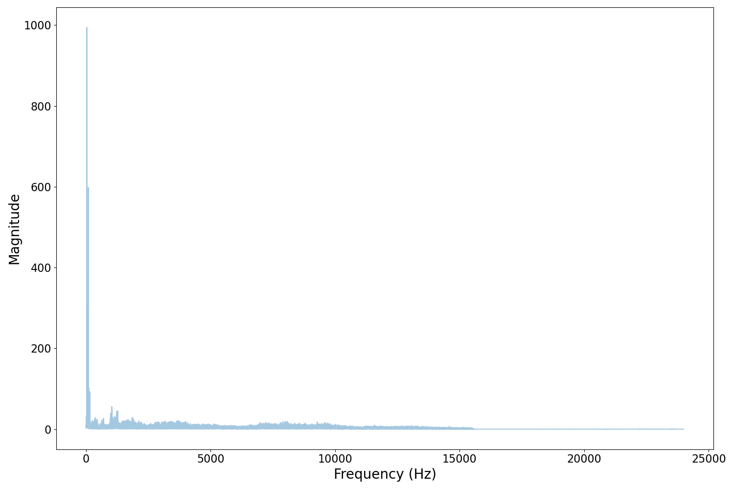
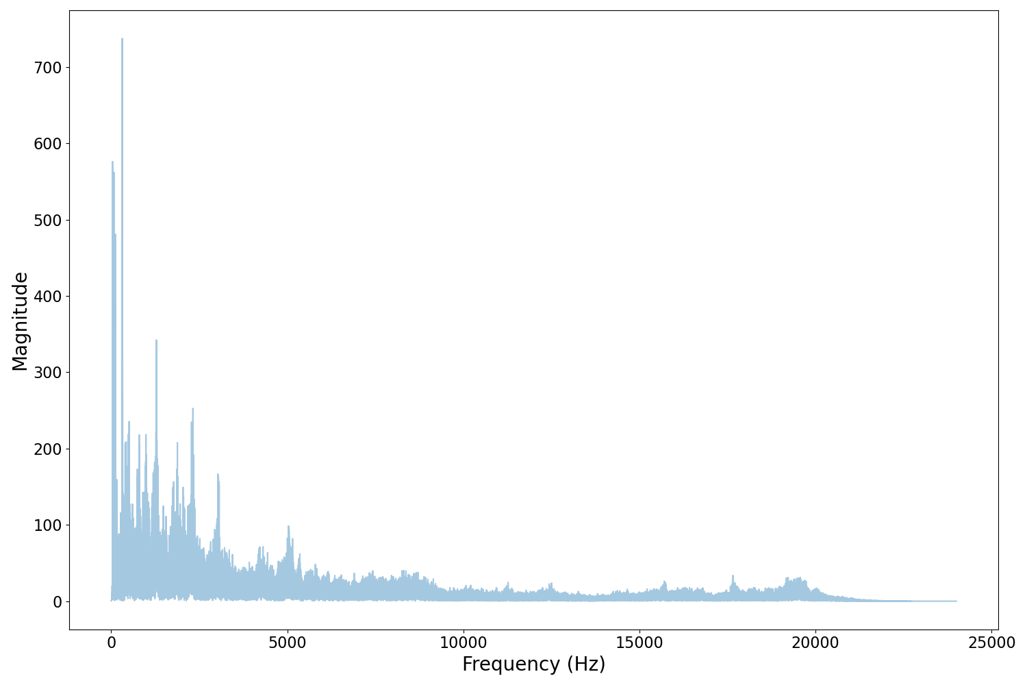
Figure 11: Example FFT - YT Sample - Frequency attenuated (left) and regular sample (right)

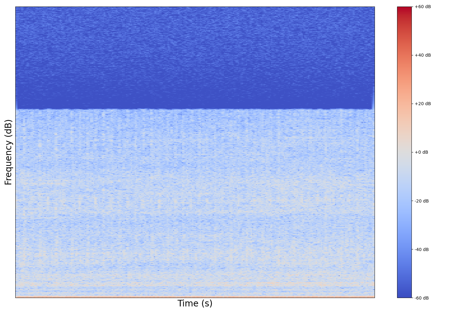
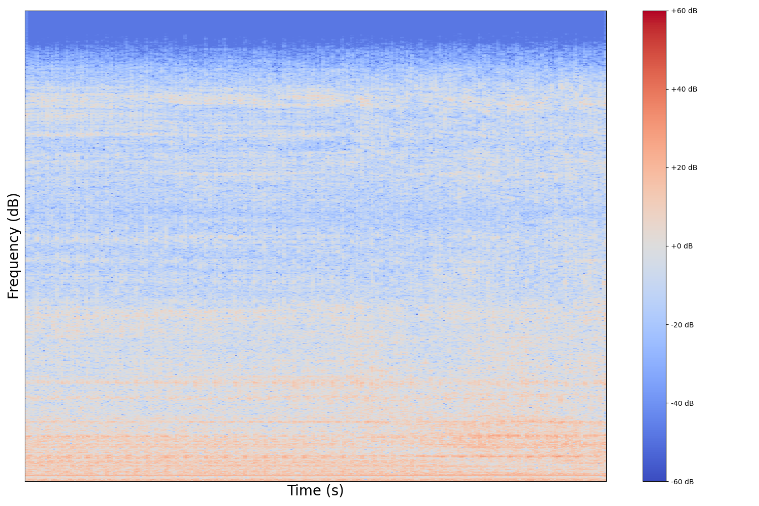
Figure 12: Example Spectrogram - YT Sample - Frequency attenuated (left) and regular sample (right)

6 Discussion

In this section we will explore three main areas of discussion:

• Broader Implications

• Future Directions

• Potential Applications

Within broader implications, we consider the larger impact our proposed architecture may have on both consumers and industry. For future directions, we note routes this work could be continued and built upon with respect to data quality, model improvement, and architectural modifications. Finally, we discuss the how our work could be utilized in diverse application areas within and outside vehicle characterization and diagnostics.

6.1 Broader Implications

There are two main groups to consider for the broader impacts of our work developing an AI mechanic: consumers and industry.

Given the end-to-end nature of our proposed system, it has practical usability for consumers to obtain vehicle status in real-time, e.g. using a mobile phone. Our high-level cascading architecture takes as input a raw audio sample, requiring no direct input or knowledge from the consumer. This has the impact of potentially saving even non-expert users stress, time, and money. Whenever their personal vehicle may be exhibiting a fault, they can receive an initial opinion from the AI mechanic. This AI mechanic could provide the consumer with insight into the seriousness of their vehicle state.

There are multiple extensions and improvements the AI mechanic may uncover when consumer data is integrated. This would create a feedback loop that would only improve the system at becoming better at detecting faults. Additionally, collection of fault data over time from long-standing consumers would create the opportunity for preventive maintenance prediction and remaining useful life (RUL) prediction. The greatest impact the AI mechanic could have on the average consumer would be helping to prevent their vehicle from exhibiting a fault in the first place through providing warnings before a fault occurs.

Prognostics will not come about immediately. For there to be value in a feedback loop from consumers, vehicles must be allowed to fail such that these data might be captured. Additionally, we showed the impact underrepresented labels have on our model and its poor outsample performance on most underrepresented labels. Without a more diverse, comprehensive, and well-balanced dataset, this behavior will still be observed. When the AI mechanic is working with a previously-unseen vehicle, it will take the system time to adjust, and may necessitate the use of techniques such as synthetic data generation or federated learning.

Within the automotive industry, off-board diagnostics which can utilize inexpensive microphones and mobile or embedded devices an alternative to the costly expense of on-board diagnostics that constantly collect and send data from the vehicle. The AI mechanic could provide automakers with an enormous swath of data on the status condition and fault identification for each kind of vehicle.

Our cascading models are flexible in that despite being trained using the vehicle attribute predictions as input to the second stage network, this could easily be adapted to take the ground truth labels as input instead. The value of this change could be significant for automakers as it would allow them to build unique fault identification models conditional upon specific vehicle types. If automakers could use inexpensive audio data to create a chart of anticipated vehicle wear, this may be used to design better vehicles and supporting infrastructure. This will require the capture and labeling of samples for desired fault identification types. If other fault types were to be integrated into the AI mechanic, this would require hundreds or thousands of distinct examples across vehicle classes to achieve similar performance to our method’s demonstrated misfire detection performance.

6.2 Future Directions

Throughout our results and ablation sections, we brought up issues with our current approach and raised potential opportunities for improvement. One of the main issues uncovered (and not unique to the AI mechanic) is the models’ dependency on quality data that is not only diverse but also balanced across classes. We showed that obtaining crowd-sourced audio data from YouTube may address data quantity, but not data quality. There is value in developing a real-world application that would make it easy for a consumer to collect data on their mobile device and store the waveform at its original $48$ kHz sampling rate to prevent lossy compression or frequency attenuation.

Another avenue for future work to address the lack of data, especially in underrepresented classes, would be generative modeling. In particular, Generative Adversarial Networks (GANs) [26] have shown great power in developing realistic samples in numerous fields, most notably facial recognition. Further exploration would be needed to understand how GANs could be extended not only to acoustic samples, but also utilized in a feedback loop for developing better synthetic samples for training, including for classes not well represented.

Another direction for improving validation and test set accuracy would be developing a better approach for feature and model fusion. Our attempts at feature fusion through concatenation by flattening of the informative 2D features were in vain. Likely a multi-lane or ensemble approach where 1D and 2D convolution can be utilized on their respective feature types should yield better overall performance. Additionally, we may consider mixup [81, 76] data augmentation as a way to improve training and generate more robust features.

There is a significant opportunity in the space of acoustic vehicle characterization. Our dataset had labels for make, OEM, idling status, recording environment/location, and more. Perhaps there could be value derived from more expansive attribute classification. Additionally, our set contains labels for horsepower and engine displacement, which would provide an interesting exploration in attribute regression.

Finally, building upon our initial proof-of-concept for a cascading architecture would be a challenging but worthwhile endeavor. It could be tackled in two main ways. The first way would be to connect more stages to the architecture both in the high-level, general acoustic classification, and low-level, fault type recognition. These additional stages may benefit from utilizing pre-trained audio embeddings and transfer learning [3, 17, 35, 24]. Additionally, extensions of existing layers may be explored to increase the level to which a system is characterized such as RUL if the status is detected as normal. The other approach, motivated by work discussed in Section 2.3, would be to implement conditional logic into the network itself. Since fault type recognition is conditional upon there being a fault in the first place, having a network which is adaptive would be a major contribution. There has already been great strides made in deep sequential networks [20] and adaptive networks focused on efficiency [73, 55, 9]. As such, building this work upon prior art would be a natural extension going forward.

6.3 Potential Applications

While our main focus of this work was on vehicle understanding, our approach and proposed cascading architecture can be adapted in broader application areas. These application areas include sequential, conditional, or multi-label prediction tasks and fault identification.

Our proposed cascading architecture is a multi-level network where each level is conditional upon the prior. Any application area where there is potential for inter-label dependency could leverage the cascading architecture. For example, music recognition has hierarchies and label dependency such as first asking does the sample contain music. Then the next stage is conditional upon the first stage where it could look to predict genre, artist, song, etc. Another area for cascading architecture could be animal recognition. Does the sample first contain an animal, then what kind of animal, what state is the animal in, what location is the animal in, is the animal behaving normally, etc.?

Not only can the cascading architecture be extended to other audio applications, but also applications with other modes of data such as in computer vision. For example, biometrics could first ascertain whether a sample contains a valid fingerprint, iris, or facial scan. Then conditionally upon the first level, it could then ask whether the biometrics scan represents a valid user, what condition the user is in, perhaps using multi-modal data such as heart rate or blood pressure prediction. Another particularly relevant example in the larger vision field is autonomous vehicles (AVs). These systems are fusing many modes of data from sensors and making certain the state of the AV would be crucial. Again it could follow the hierarchy of does the sample contain an AV, what are the attributes of the AV, is the AV behaving normally, and if not what fault behavior is the AV?

The other significant application area for these techniques is broader fault identification, particularly using audio data. This includes other diagnostic areas, such as for industrial processes or energy sector equipment. One such example is home or industrial heating and ventilation systems: in this case, we first ask can we identify whether a sample contains ventilation equipment using acoustic classification networks. Then we would look to obtain its operating state and condition. If it’s behaving normally, what is expected RUL? If abnormal, what is the fault type and degree?

This cascading architecture can be extended to any application where a fault might occur. Some of these may include home appliances (washer/dryer) with belt slipping or drum imbalance, electric cars / bicycles with suspension issues, manufacturing equipment (CNC mills/lathes) with tool run-out or spindle issues, drills with brush wear or belt slip, the energy sector with turbine and pump health, elevator / escalators condition, and even carnival / fair equipment.

In summary, our proposed method is broadly applicable to any task which can leverage a conditional dependency and/or has a potential need for fault identification. We plan to explore the identified areas and more in continuations of this work.

7 Conclusion

In this manuscript, we took the first steps towards building an AI mechanic. We identified four main areas of novelty with our work:

• Sound Recognition using Deep Learning: We demonstrated the value and need for vehicle understanding as an application domain for sound recognition using deep learning. More specifically, we know the world is becoming ever dependent upon transportation. Sound is a prevalent and inexpensive resource. Fault detection is a lengthy and time-consuming endeavor even for expert mechanics. Through an AI mechanic that can listen to a vehicle, we can utilize a cost-effective solution that can improve lives by reducing vehicle emissions and increasing usable service life.
  

  By developing knowledge and capabilities in support of identifying systems with expert level detail, without expert knowledge, we reduce barriers to instrumentation that today stand in the way of proactive and reactive maintenance operations. Our solution will help individuals, fleet managers, and third parties to instrument vehicles more comprehensively and effectively than is presently feasible. The net result of this increased insight and transparency will be a more efficient, reliable, and safer fleet.
  

• Acoustic Vehicle Characterization: We showcased the first published results on the engine configuration attribute task, to the best of our knowledge. Improving on prior work, we built an all-in-one model for all four attribute types. Additionally, we employed multi-task learning for both the attributes and misfire prediction tasks to better inform one another. We also merged the attributes and misfire datasets which created a larger and more challenging dataset to predict attributes on both normally and abnormally performing samples.
  

• Cascading Architectures: We defined cascading architectures as sequential, multi-level, conditional networks. As a proof-of-concept, we built a two-stage convolutional neural network where the first stage specialized on vehicle attributes and then cascaded its attribute predictions to the second stage which specialized on misfire detection with the goal of better informing both prediction tasks.
  

  This two-stage cascading network demonstrated strong performance of $95.6\%$, $93.7\%$, $94.0\%$, and $92.8\%$ validation accuracy on the fuel type, engine configuration, cylinder count, and aspiration type prediction tasks, respectively. In comparing across a naïve and parallel baseline, the cascading model showcased $16.4\%$ and $4.2\%$, respectively, relative improvement on misfire fault prediction with a validation accuracy of $93.6\%$. Additionally, the cascading model achieved $86.8\%$ test set accuracy on misfire fault prediction, demonstrating margins of $7.8\%$ and $1.5\%$ improvement over naïve and parallel baselines.
  

• Audio Data Augmentation: We constructed a vast acoustic vehicle characterization dataset with over 50k samples for over 40 hours of audio using data augmentation techniques. Through ablation studies, we establish the positive impact data augmentation has on outsample generalizability. We additionally show the limitations of crowd-sourced audio from YouTube to further support the value our augmented dataset provides to the community.
  

We concluded our manuscript with an important discussion of the broader implications, future directions, and potential applications of the AI mechanic, highlighting the potential for future research and adoption of the developed architectures and concepts.

References

- [1] Ossama Abdel-Hamid, Abdel-rahman Mohamed, Hui Jiang, Li Deng, Gerald Penn, and Dong Yu. Convolutional neural networks for speech recognition. IEEE/ACM Transactions on audio, speech, and language processing, 22(10):1533–1545, 2014.
- [2] Jakob Abeßer. A review of deep learning based methods for acoustic scene classification. Applied Sciences, 10(6), 2020.
- [3] Relja Arandjelovic and Andrew Zisserman. Look, listen and learn. In Proceedings of the IEEE International Conference on Computer Vision, pages 609–617, 2017.
- [4] Muhammad Ahsan Aslam, Muhammad Umer Sarwar, Muhammad Kashif Hanif, Ramzan Talib, and Usama Khalid. Acoustic classification using deep learning. Int. J. Adv. Comput. Sci. Appl, 9(8):153–159, 2018.
- [5] Soo Hyun Bae, Inkyu Choi, and Nam Soo Kim. Acoustic scene classification using parallel combination of lstm and cnn. In Proceedings of the Detection and Classification of Acoustic Scenes and Events 2016 Workshop (DCASE2016), pages 11–15, 2016.
- [6] Saeed Asadi Bagloee, Madjid Tavana, Mohsen Asadi, and Tracey Oliver. Autonomous vehicles: challenges, opportunities, and future implications for transportation policies. Journal of modern transportation, 24(4):284–303, 2016.
- [7] Ohad Barak and Nizar Sallem. Audio data augmentation for road objects classification by an artificial neural network. In Audio Engineering Society Convention 147. Audio Engineering Society, 2019.
- [8] Daniele Battaglino, Ludovick Lepauloux, Nicholas Evans, France Mougins, and France Biot. Acoustic scene classification using convolutional neural networks. IEEE AASP Challenge on Detec, 2016.
- [9] Emmanuel Bengio, Pierre-Luc Bacon, Joelle Pineau, and Doina Precup. Conditional computation in neural networks for faster models. arXiv preprint arXiv:1511.06297, 2015.
- [10] Keshav Bimbraw. Autonomous cars: Past, present and future a review of the developments in the last century, the present scenario and the expected future of autonomous vehicle technology. In 2015 12th international conference on informatics in control, automation and robotics (ICINCO), volume 1, pages 191–198. IEEE, 2015.
- [11] Francisco J Bravo Sanchez, Md Rahat Hossain, Nathan B English, and Steven T Moore. Bioacoustic classification of avian calls from raw sound waveforms with an open-source deep learning architecture. Scientific Reports, 11(1):1–12, 2021.
- [12] Chloë Brown, Jagmohan Chauhan, Andreas Grammenos, Jing Han, Apinan Hasthanasombat, Dimitris Spathis, Tong Xia, Pietro Cicuta, and Cecilia Mascolo. Exploring automatic diagnosis of covid-19 from crowdsourced respiratory sound data. arXiv preprint arXiv:2006.05919, 2020.
- [13] Seok-Jun Bu, Hyung-Jun Moon, and Sung-Bae Cho. Adversarial signal augmentation for cnn-lstm to classify impact noise in automobiles. In 2021 IEEE International Conference on Big Data and Smart Computing (BigComp), pages 60–64. IEEE, 2021.
- [14] Haoze Chen and Zhijie Zhang. Hybrid neural network based on novel audio feature for vehicle type identification. Scientific Reports, 11(1):1–10, 2021.
- [15] Tien-En Chen, Shih-I Yang, Li-Ting Ho, Kun-Hsi Tsai, Yu-Hsuan Chen, Yun-Fan Chang, Ying-Hui Lai, Syu-Siang Wang, Yu Tsao, and Chau-Chung Wu. S1 and s2 heart sound recognition using deep neural networks. IEEE Transactions on Biomedical Engineering, 64(2):372–380, 2016.
- [16] Umberto Coda. Artificial intelligence for vehicle engine classification and vibroacoustic diagnostics. Master’s thesis, Politecnico di Torino, Oct 2020.
- [17] Jason Cramer, Ho-Hsiang Wu, Justin Salamon, and Juan Pablo Bello. Look, listen, and learn more: Design choices for deep audio embeddings. In ICASSP 2019-2019 IEEE International Conference on Acoustics, Speech and Signal Processing (ICASSP), pages 3852–3856. IEEE, 2019.
- [18] Wei Dai, Chia Dai, Shuhui Qu, Juncheng Li, and Samarjit Das. Very deep convolutional neural networks for raw waveforms. In 2017 IEEE International Conference on Acoustics, Speech and Signal Processing (ICASSP), pages 421–425. IEEE, 2017.
- [19] Avi Dascalu and EO David. Skin cancer detection by deep learning and sound analysis algorithms: A prospective clinical study of an elementary dermoscope. EBioMedicine, 43:107–113, 2019.
- [20] Ludovic Denoyer and Patrick Gallinari. Deep sequential neural network. arXiv preprint arXiv:1410.0510, 2014.
- [21] Linhao Dong, Shuang Xu, and Bo Xu. Speech-transformer: a no-recurrence sequence-to-sequence model for speech recognition. In 2018 IEEE International Conference on Acoustics, Speech and Signal Processing (ICASSP), pages 5884–5888. IEEE, 2018.
- [22] Jürgen T Geiger, Björn Schuller, and Gerhard Rigoll. Large-scale audio feature extraction and svm for acoustic scene classification. In 2013 IEEE Workshop on Applications of Signal Processing to Audio and Acoustics, pages 1–4. IEEE, 2013.
- [23] Jort F Gemmeke, Daniel PW Ellis, Dylan Freedman, Aren Jansen, Wade Lawrence, R Channing Moore, Manoj Plakal, and Marvin Ritter. Audio set: An ontology and human-labeled dataset for audio events. In 2017 IEEE international conference on acoustics, speech and signal processing (ICASSP), pages 776–780. IEEE, 2017.
- [24] Yuan Gong, Yu-An Chung, and James Glass. Ast: Audio spectrogram transformer. arXiv preprint arXiv:2104.01778, 2021.
- [25] Ian Goodfellow, Yoshua Bengio, and Aaron Courville. Deep learning. MIT press, 2016.
- [26] Ian Goodfellow, Jean Pouget-Abadie, Mehdi Mirza, Bing Xu, David Warde-Farley, Sherjil Ozair, Aaron Courville, and Yoshua Bengio. Generative adversarial nets. Advances in neural information processing systems, 27, 2014.
- [27] Alex Graves and Navdeep Jaitly. Towards end-to-end speech recognition with recurrent neural networks. In International conference on machine learning, pages 1764–1772. PMLR, 2014.
- [28] Alex Graves, Abdel-rahman Mohamed, and Geoffrey Hinton. Speech recognition with deep recurrent neural networks. In 2013 IEEE international conference on acoustics, speech and signal processing, pages 6645–6649. Ieee, 2013.
- [29] Anmol Gulati, James Qin, Chung-Cheng Chiu, Niki Parmar, Yu Zhang, Jiahui Yu, Wei Han, Shibo Wang, Zhengdong Zhang, Yonghui Wu, et al. Conformer: Convolution-augmented transformer for speech recognition. arXiv preprint arXiv:2005.08100, 2020.
- [30] Shawn Hershey, Sourish Chaudhuri, Daniel PW Ellis, Jort F Gemmeke, Aren Jansen, R Channing Moore, Manoj Plakal, Devin Platt, Rif A Saurous, Bryan Seybold, et al. Cnn architectures for large-scale audio classification. In 2017 ieee international conference on acoustics, speech and signal processing (icassp), pages 131–135. IEEE, 2017.
- [31] Jonathan Huang, Hong Lu, Paulo Lopez Meyer, Hector Cordourier, and Juan Del Hoyo Ontiveros. Acoustic scene classification using deep learning-based ensemble averaging, 2019.
- [32] Max Jaderberg, Karen Simonyan, Andrew Zisserman, et al. Spatial transformer networks. Advances in neural information processing systems, 28:2017–2025, 2015.
- [33] Il-Young Jeong and Kyogu Lee. Learning temporal features using a deep neural network and its application to music genre classification. In Ismir, pages 434–440, 2016.
- [34] Tom Ko, Vijayaditya Peddinti, Daniel Povey, and Sanjeev Khudanpur. Audio augmentation for speech recognition. In Sixteenth annual conference of the international speech communication association, 2015.
- [35] Qiuqiang Kong, Yin Cao, Turab Iqbal, Yuxuan Wang, Wenwu Wang, and Mark D Plumbley. Panns: Large-scale pretrained audio neural networks for audio pattern recognition. IEEE/ACM Transactions on Audio, Speech, and Language Processing, 28:2880–2894, 2020.
- [36] TK Landauer, CA Kamm, and S Singhal. Learning a minimally structured back propagation network to recognize speech. In Proc. of the Ninth Annual Conf. of the Cognitive Science Society, pages 531–536, 1987.
- [37] Yann LeCun, Yoshua Bengio, and Geoffrey Hinton. Deep learning. nature, 521(7553):436–444, 2015.
- [38] Cheng-Hsiung Lee, Jung-Sing Jwo, Han-Yi Hsieh, and Ching-Sheng Lin. An intelligent system for grinding wheel condition monitoring based on machining sound and deep learning. IEEE Access, 8:58279–58289, 2020.
- [39] Hongmei Liu, Lianfeng Li, and Jian Ma. Rolling bearing fault diagnosis based on stft-deep learning and sound signals. Shock and Vibration, 2016, 2016.
- [40] Oisin Mac Aodha, Rory Gibb, Kate E Barlow, Ella Browning, Michael Firman, Robin Freeman, Briana Harder, Libby Kinsey, Gary R Mead, Stuart E Newson, et al. Bat detective—deep learning tools for bat acoustic signal detection. PLoS computational biology, 14(3):e1005995, 2018.
- [41] Dimos Makris, Maximos Kaliakatsos-Papakostas, and Katia Lida Kermanidis. Deepdrum: An adaptive conditional neural network. arXiv preprint arXiv:1809.06127, 2018.
- [42] Ian McLoughlin, Haomin Zhang, Zhipeng Xie, Yan Song, Wei Xiao, and Huy Phan. Continuous robust sound event classification using time-frequency features and deep learning. PloS one, 12(9):e0182309, 2017.
- [43] Fady Medhat, David Chesmore, and John Robinson. Masked conditional neural networks for sound classification. Applied Soft Computing, 90:106073, 2020.
- [44] Loris Nanni, Gianluca Maguolo, and Michelangelo Paci. Data augmentation approaches for improving animal audio classification. Ecological Informatics, 57:101084, 2020.
- [45] Sergio Oramas, Francesco Barbieri, Oriol Nieto Caballero, and Xavier Serra. Multimodal deep learning for music genre classification. Transactions of the International Society for Music Information Retrieval. 2018; 1 (1): 4-21., 2018.
- [46] Arjun Pakrashi and Brian Mac Namee. Cascademl: An automatic neural network architecture evolution and training algorithm for multi-label classification (best technical paper). In International Conference on Innovative Techniques and Applications of Artificial Intelligence, pages 3–17. Springer, 2019.
- [47] Dimitri Palaz, Ronan Collobert, et al. Analysis of cnn-based speech recognition system using raw speech as input. Technical report, Idiap, 2015.
- [48] Iliana Papamichael, Georgios Pappas, Joshua E Siegel, and Antonis A Zorpas. Unified waste metrics: A gamified tool in next-generation strategic planning. Science of The Total Environment, page 154835, 2022.
- [49] Taxonomy SAE. Definitions for terms related to shared mobility and enabling technologies, 2018.
- [50] Justin Salamon and Juan Pablo Bello. Deep convolutional neural networks and data augmentation for environmental sound classification. IEEE Signal processing letters, 24(3):279–283, 2017.
- [51] Jan Schlüter and Thomas Grill. Exploring data augmentation for improved singing voice detection with neural networks. In ISMIR, pages 121–126, 2015.
- [52] Roneel V Sharan and Tom J Moir. Robust acoustic event classification using deep neural networks. Information Sciences, 396:24–32, 2017.
- [53] Muddsair Sharif, Mayur Hotwani, Seker Huseyin, and Gero Lückemeyer. imobilakou: The role of machine listening to detect vehicle using sound acoustics., 2021.
- [54] Garima Sharma, Kartikeyan Umapathy, and Sridhar Krishnan. Trends in audio signal feature extraction methods. Applied Acoustics, 158:107020, 2020.
- [55] Noam Shazeer, Azalia Mirhoseini, Krzysztof Maziarz, Andy Davis, Quoc Le, Geoffrey Hinton, and Jeff Dean. Outrageously large neural networks: The sparsely-gated mixture-of-experts layer. arXiv preprint arXiv:1701.06538, 2017.
- [56] Joshua Siegel. Automotive engine air filter audio samples - free flowing, contaminated and obstructed samples, 2017.
- [57] Joshua Siegel, Rahul Bhattacharyya, Sanjay Sarma, and Ajay Deshpande. Smartphone-based vehicular tire pressure and condition monitoring. In Yaxin Bi, Supriya Kapoor, and Rahul Bhatia, editors, Proceedings of SAI Intelligent Systems Conference (IntelliSys) 2016, pages 805–824, Cham, 2018. Springer International Publishing.
- [58] Joshua Siegel, Umberto Coda, and Adam Terwilliger. Surveying off-board and extra-vehicular monitoring and progress towards pervasive diagnostics. SAE International Journal of Connected and Automated Vehicles, 2021.
- [59] Joshua Siegel, Sumeet Kumar, Isaac Ehrenberg, and Sanjay Sarma. Engine misfire detection with pervasive mobile audio. In Bettina Berendt, Björn Bringmann, Élisa Fromont, Gemma Garriga, Pauli Miettinen, Nikolaj Tatti, and Volker Tresp, editors, Machine Learning and Knowledge Discovery in Databases, pages 226–241, Cham, 2016. Springer International Publishing.
- [60] Joshua E. Siegel, Rahul Bhattacharyya, Sumeet Kumar, and Sanjay E. Sarma. Air filter particulate loading detection using smartphone audio and optimized ensemble classification. Engineering Applications of Artificial Intelligence, 66:104 – 112, 2017.
- [61] Joshua E Siegel, Rahul Bhattacharyya, Sanjay Sarma, and Ajay Deshpande. Smartphone-based wheel imbalance detection. In Dynamic Systems and Control Conference, volume 57250, page V002T19A002. American Society of Mechanical Engineers, 2015.
- [62] Joshua E. Siegel, Shane Pratt, Yongbin Sun, and Sanjay E. Sarma. Real-time deep neural networks for internet-enabled arc-fault detection. Engineering Applications of Artificial Intelligence, 74:35–42, 2018.
- [63] Joshua E. Siegel, Yongbin Sun, and Sanjay Sarma. Automotive diagnostics as a service: An artificially intelligent mobile application for tire condition assessment. In Marco Aiello, Yujiu Yang, Yuexian Zou, and Liang-Jie Zhang, editors, Artificial Intelligence and Mobile Services – AIMS 2018, pages 172–184, Cham, 2018. Springer International Publishing.
- [64] Dan Stowell, Michael D Wood, Hanna Pamuła, Yannis Stylianou, and Hervé Glotin. Automatic acoustic detection of birds through deep learning: the first bird audio detection challenge. Methods in Ecology and Evolution, 10(3):368–380, 2019.
- [65] Yiwei Sun and Shabnam Ghaffarzadegan. An ontology-aware framework for audio event classification. In ICASSP 2020-2020 IEEE International Conference on Acoustics, Speech and Signal Processing (ICASSP), pages 321–325. IEEE, 2020.
- [66] Ian Tiseo. Passenger car carbon dioxide emissions worldwide 2010-2020, Dec 2021.
- [67] Rafael Torres, Daniele Battaglino, and Ludovick Lepauloux. Baby cry sound detection: A comparison of hand crafted features and deep learning approach. In International Conference on Engineering Applications of Neural Networks, pages 168–179. Springer, 2017.
- [68] John Voelcker. 1.2 billion vehicles on world’s roads now, 2 billion by 2035: Report, Jul 2014.
- [69] Elias Wang, Atli Kosson, and Tong Mu. Deep action conditional neural network for frame prediction in atari games. Technical report, Technical Report, Stanford University, 2017.
- [70] Qiurui Wang, Chun Yuan, and Yan Liu. Learning deep conditional neural network for image segmentation. IEEE Transactions on Multimedia, 21(7):1839–1852, 2019.
- [71] Yongqiang Wang, Abdelrahman Mohamed, Due Le, Chunxi Liu, Alex Xiao, Jay Mahadeokar, Hongzhao Huang, Andros Tjandra, Xiaohui Zhang, Frank Zhang, et al. Transformer-based acoustic modeling for hybrid speech recognition. In ICASSP 2020-2020 IEEE International Conference on Acoustics, Speech and Signal Processing (ICASSP), pages 6874–6878. IEEE, 2020.
- [72] Zheng Weiping, Yi Jiantao, Xing Xiaotao, Liu Xiangtao, and Peng Shaohu. Acoustic scene classification using deep convolutional neural network and multiple spectrograms fusion. Detection and Classification of Acoustic Scenes and Events (DCASE), 2017.
- [73] Zuxuan Wu, Tushar Nagarajan, Abhishek Kumar, Steven Rennie, Larry S. Davis, Kristen Grauman, and Rogerio Feris. Blockdrop: Dynamic inference paths in residual networks. In Proceedings of the IEEE Conference on Computer Vision and Pattern Recognition (CVPR), June 2018.
- [74] Jie Xie and Mingying Zhu. Handcrafted features and late fusion with deep learning for bird sound classification. Ecological Informatics, 52:74–81, 2019.
- [75] Chao Xiong, Xiaowei Zhao, Danhang Tang, Karlekar Jayashree, Shuicheng Yan, and Tae-Kyun Kim. Conditional convolutional neural network for modality-aware face recognition. In Proceedings of the IEEE International Conference on Computer Vision (ICCV), December 2015.
- [76] Kele Xu, Dawei Feng, Haibo Mi, Boqing Zhu, Dezhi Wang, Lilun Zhang, Hengxing Cai, and Shuwen Liu. Mixup-based acoustic scene classification using multi-channel convolutional neural network. In Pacific Rim conference on multimedia, pages 14–23. Springer, 2018.
- [77] An-Chih Yang and Emmett D Goodman. Audio classification of accelerating vehicles, 2019.
- [78] Hao Yang, Chunfeng Yuan, Junliang Xing, and Weiming Hu. Scnn: Sequential convolutional neural network for human action recognition in videos. In 2017 IEEE International Conference on Image Processing (ICIP), pages 355–359. IEEE, 2017.
- [79] G. Zavaliagkos, Y. Zhao, R. Schwartz, and J. Makhoul. A hybrid segmental neural net/hidden markov model system for continuous speech recognition. IEEE Transactions on Speech and Audio Processing, 2(1):151–160, 1994.
- [80] Andrej Zgank. Iot-based bee swarm activity acoustic classification using deep neural networks. Sensors, 21(3):676, 2021.
- [81] Hongyi Zhang, Moustapha Cisse, Yann N. Dauphin, and David Lopez-Paz. mixup: Beyond empirical risk minimization. In International Conference on Learning Representations, 2018.
- [82] Ming Zhong, Manuel Castellote, Rahul Dodhia, Juan Lavista Ferres, Mandy Keogh, and Arial Brewer. Beluga whale acoustic signal classification using deep learning neural network models. The Journal of the Acoustical Society of America, 147(3):1834–1841, 2020.