Electromagnetic precursor flares from the late inspiral of neutron star binaries

Abstract

The coalescence of two neutron stars is accompanied by the emission of gravitational waves, and can also feature electromagnetic counterparts powered by mass ejecta and the formation of a relativistic jet after the merger. Since neutron stars can feature strong magnetic fields, the non-trivial interaction of the neutron star magnetospheres might fuel potentially powerful electromagnetic transients prior to merger. A key process powering those precursor transients is relativistic reconnection in strong current sheets formed between the two stars. In this work, we provide a detailed analysis of how the twisting of the common magnetosphere of the binary leads to an emission of electromagnetic flares, akin to those produced in the solar corona. By means of relativistic force-free electrodynamics simulations, we clarify the role of different magnetic field topologies in the process. We conclude that flaring will always occur for suitable magnetic field alignments, unless one of the neutron stars has a magnetic field significantly weaker than the other.

I Introduction

With the discovery of gravitational waves from coalescing black holes [1, 2, 3, 4, 5, 6, 7, 8, 9, 10, 11, 12] (see also, e.g., [13, 14, 15]), binary neutron star [16, 17] and black hole – neutron star [11, 18, 12] systems, we have entered a new era of compact object science. Especially the matter present in the latter two systems, has the potential to fuel electromagnetic counterparts, which where observed for the GW170817 event( e.g. [19, 20, 21, 22, 23, 24, 25, 26]). This makes the search for electromagnetic counterparts an integral part of any gravitational wave detection. While the first detection of a neutron star binary coalescence was accompanied by two distinct counterparts [19], likely originating during and after merger, there could be yet another counterpart emitted right before merger [27, 28, 29]. Such a precursor is thought to arise due to interactions of magnetic flux tubes in the pair-plasma filled common magnetosphere of the binary [28],which requires the presence a steady magnetic field anchored in matter. Hence, making binary neutron star and black hole – neutron star collisions prime targets to detect such precursors [30]. Indeed, in the case of black hole – neutron star mergers, electromagnetic precursors might also be the only accompanying transient if the neutron star is swallowed whole, see e.g. [31, 32, 33, 34, 35]. As such, precursors are also potential candidates for powerful radio signals (e.g., [33, 36]). The prospects for creating early warning systems for electromagnetic follow-up observations of precursor emission has recently been investigated [37, 38, 39], crucial for their potential future detection [40]. For the event GW170817 attempts have even been made to detect precursor emission [30, 41], see also [42, 43]. Coincident detection of precursor emission could also be used to (further) constrain the sky localization of the merger site[44].

A variety of models have been proposed for the production of precursors to compact binary mergers. These include explosive fireball models [45], gamma-ray flares [46, 47], shock-powered radio precursors [48], unipolar inductors [49, 50], crustal shattering [46]. Particular examples of reconnection-based models include Refs. [51, 52] , where dissipation in (transient) current sheets powers the emission. Especially the latter class of models requires a non-linear interaction of magnetic fields in reconnecting current sheet, whose boundary conditions are determined by the global dynamics of the problem [53]. This motivates the need for global numerical simulations of the magnetospheric dynamics in a close compact binary. To study the precursor emission mechanism numerically different types of simulations have been performed. In particular, simulations in special-relativistic force-free electrodynamics have clarified the emission of single orbiting neutron stars [54], idealized mixed binaries [55], and magnetospheric interaction in binary neutron star systems [51]. Studies in dynamical spacetimes have focused on understanding electromagnetic bursts produced from single neutron stars, either in isolation [56], or as mimickers for post-merger remnants [57]. A small number of studies has also focused on the magnetospheric dynamics during the collapse [58, 59, 60] and collision of neutron stars [61], where their magnetospheres were inactive. Full general-relativistic simulations of force-free electrodynamics have been conducted to better understand the common magnetosphere prior to merger, see, e.g., for black hole binaries [62, 63, 64, 65], neutron star binaries [66, 67, 68], and mixed systems [69, 70]. While several numerical formulations of relativistic force-free electrodynamics have been proposed (e.g., [71, 72, 56, 73, 74, 75, 76]), most of the simulations mentioned above have used a variation of independently evolving electric and magnetic fields according to the relativistic Maxwell equations [77, 56]. The latter is supplemented by a suitable prescription for the electric current mimicking a (resistive) force-free pair plasma (see, e.g., Refs. [78, 79, 80] for a recent discussion).

In this work, we extend our initial findings [51] for the flaring process in the common magnetosphere of neutron star binaries in close contact. Using special-relativistic force-free electrodynamics simulations, we present a set of models focusing on the impact of magnetic field topology on the emission of the flares and the viability of their production mechanism. We clarify, in particular, that the emission of flares is largely insensitive to magnetic field alignments and unequal field strengths, as long as there is a significant component of the magnetic moment pointing in each hemisphere.

This paper is structures as follows: In Sec. II we provide a detailed overview of the numerical methods and analysis tools used in this work. In our main Sec. III we provide a detailed description of the numerical simulations presented in this work. We conclude with a short discussion in Sec. IV.
Unless otherwise indicated, we use geometrical units $c=G=k_{B}=1$.

II Methods

We study the production of electromagnetic flares launched from an orbiting neutron star binary in close contact. We assume that the induced electric field at the surface of either neutron star are sufficiently large to trigger an electron positron pair cascade [81], hence, filling the immediate surrounding of the binary with a force-free highly conductive plasma [27, 28, 29]. This allows us to model the binary using relativistic force-free electrodynamics in a flat corotating space-time following the approaches taken in [54, 51].
In the following, we will briefly summarize the equations of force-free electrodynamics, the setup of the binary system, and the numerical implementation.

II.1 Relativistic electrodynamics

In this section, we want to review the equations of general-relativistic electrodynamics [82, 56]. The four-dimensional spacetime metric $g_{\mu\nu}$ can be expressed within the 3+1 split as follows [83],

$${\rm d}s^{2}= g_{\mu\nu}{\rm d}x^{\mu}{\rm d}x^{\nu}$$

$$= \left(-\alpha^{2}+\beta_{k}\beta^{k}\right){\rm d}t^{2}+2\beta_{k}{\rm d}x^{k}{\rm d}t+\gamma_{ij}{\rm d}x^{i}{\rm d}x^{j},$$ (1)

where $\alpha$ and $\beta^{i}$ are the lapse and shift respectively. This decomposition introduces spatial hypersurfaces characterized by the normal vector $n_{\mu}=\left(-\alpha,0,0,0\right)$. Within this work, we will adopt a corotating flat frame, in which $\alpha=1$ and $\gamma_{ij}=\delta_{ij}$, but non-zero shift $\beta^{k}$. We will specify the precise choice of $\beta^{k}$ in Sec. II.2, see also [54, 51]. The dynamics of electromagnetic fields in relativity is governed by the generalized form of Maxwell’s equations [56],

$$\nabla_{\mu}\left(F^{\mu\nu}+\phi g^{\mu\nu}\right) =-4\pi\mathcal{J}^{\nu}+\kappa_{\phi}n^{\nu}\phi,$$ (2)

$$\nabla_{\mu}\left({}^{\ast}F^{\mu\nu}+\psi g^{\mu\nu}\right) =+\kappa_{\psi}n^{\nu}\psi\,,$$ (3)

$$\nabla_{\mu}\mathcal{J}^{\mu} =0\,.$$ (4)

These equations are written in terms of the four-dimensional spacetime metric $g_{\mu\nu}$, the field strength tensor $F^{\mu\nu}$ and its dual ${}^{\ast}F^{\mu\nu}=\frac{1}{2}\varepsilon^{\mu\nu\kappa\lambda}F_{\kappa\lambda}$, where $\varepsilon^{\mu\nu\kappa\lambda}$ is the Levi-Civita tensor. In order to preserve the divergence-free condition of the magnetic field, as well as consistency of the separately evolved charge density with the electric field, we have added divergence cleaning scalars $\phi$ and $\psi$ with corresponding dissipation coefficients $\kappa_{\phi/\psi}$ [84]. We note that these extra fields vanish in the continuum limit, and that there presence requires to separately impose charge conservation via Eq. (3). For this choice of lapse, we obtain that the electromagnetic fields and currents are given by [56]

$$B^{\mu} =-n_{\nu}\,{{}^{\ast}}F^{\mu\nu},$$ (5)

$$E^{\mu} =-n_{\nu}F^{\mu\nu},$$ (6)

$$q =-n_{\nu}\mathcal{J}^{\nu},$$ (7)

$$J^{\mu} =h^{\mu}_{\nu}\mathcal{J}^{\nu},$$ (8)

where we have defined the electric field $E^{\mu}=\left(0,E^{i}\right)$, the magnetic field $B^{\mu}=\left(0,B^{i}\right)$, the charge density $q$ and the current $J^{\mu}=\left(0,J^{i}\right)$. We have further introduced the projector $h_{\mu\nu}=g_{\mu\nu}+n_{\mu}n_{\nu}$. Expanding out the Maxwell equations (2) and (3) we obtain,

$$\partial_{t}B^{i}+\partial_{k}\left(-\beta^{k}B^{i}+\varepsilon^{ikj}E_{j}+\phi\delta^{ik}\right) =-B^{k}\partial_{k}\beta^{i},$$ (10)

$$\partial_{t}E^{i}+\partial_{k}\left(-\beta^{k}E^{i}-\varepsilon^{ikj}B_{j}+\psi\delta^{ik}\right) =-E^{k}\partial_{k}\beta^{i}-4\pi J^{i},$$ (11)

$$\partial_{t}\psi+\partial_{k}\left(-\beta^{k}\psi+E^{k}\right) =q-\kappa_{\psi}\psi.$$ (12)

$$\partial_{t}\phi+\partial_{k}\left(-\beta^{k}\phi+B^{k}\right) =-\kappa_{\phi}\phi,$$ (13)

$$\partial_{t}q+\partial_{i}\left(-\beta^{i}q+J^{i}\right) =0.$$ (14)

	$f_{1}\left[\rm Hz\right]$	$f_{2}\left[\rm Hz\right]$	$\Omega/2\pi\left[\rm Hz\right]$	$\mathcal{Q}_{0}\,\left[\rm km\right]$	$B_{\rm 2}/B_{\rm 1}$	$\theta_{1}$	$\theta_{2}$	$\phi$	$a\,\left[\rm km\right]$
A0 $\left(\downarrow\nearrow\,0^{\circ}\right)$	–	–	259	–	1.9	0	180	0	52
A30 $\left(\downarrow\nearrow\,30^{\circ}\right)$	–	–	259	–	1.9	0	150	0	52
A60$\left(\downarrow\nearrow\,60^{\circ}\right)$	–	–	259	–	1.9	0	120	0	52
A90$\left(\downarrow\nearrow\,90^{\circ}\right)$	–	–	259	–	1.9	0	90	0	52
O0 $\left(\nearrow\swarrow\right)$	–	–	259	–	1.9	0	120	0	52
O180 $\left(\nearrow\searrow\right)$	–	–	259	–	1.9	0	120	180	52
Q$\uparrow\uparrow$	–	–	259	44	1	0	30	0	52
Q${}^{\ast}\uparrow\uparrow$	–	–	259	82	1	0	30	0	52
Q$\downarrow\downarrow$	–	–	259	44	1	0	120	0	52
U0$\left(\nwarrow\swarrow\,1:1\right)$	–	100	259	–	1.9	30	150	0	52
U3$\left(\nwarrow\swarrow\,1:3\right)$	–	100	259	–	0.636	30	150	0	52
U9$\left(\nwarrow\swarrow\,1:9\right)$	–	100	259	–	0.121	30	150	0	52
U27 $\left(\nwarrow\swarrow\,1:27\right)$	–	100	259	–	0.071	30	150	0	52

Table 1: Summary of the neutron star binaries considered in this work. The columns denote the spin frequencies of the stars $f_{\rm 1/2}$, the orbital spin frequency $\Omega$, the relative maximum magnetic field strengths $B_{2}/B_{1}$ at the surface of the stars, the inclination $\theta_{1/2}$, the relative initial offset $\phi$ between the two stars and the separation $a$. We further use $\mathcal{Q}_{0}$ to denote strength of the quadrupolar component, where applicable. In the decoupling limit between the electromagnetic field and the gravitational sector that we consider in this work, the magnetic field strength $B_{1}$ can be arbitrarily re-scaled, so that no explicit value needs to be provided. For the actual simulations, we use $B_{1}=1.9\,\times 10^{12}\,\rm G$.

We recall that the relativistic energy momentum tensor for electric and magnetic fields is given by [82],

$$4\pi T_{\rm EM}^{\mu\nu}= \frac{1}{2}\left[E^{2}+B^{2}\right]g^{\mu\nu}+2n^{(\mu}\varepsilon^{\nu)\kappa\lambda}E_{\kappa}B_{\lambda}$$

$$-E^{\mu}E^{\nu}-B^{\mu}B^{\nu}\,,$$ (15)

where $\varepsilon^{\mu\nu\kappa\lambda}$ is the four-dimensional Levi-Civita tensor and $2A^{(\mu}B^{\nu)}=A^{\mu}B^{\nu}+B^{\mu}A^{\nu}$. The electromagnetic energy density $\rho_{\rm EM}$ can then be recovered by contracting $T_{\rm EM}^{\mu\nu}$ with the normal vector $n_{\mu}$,viz. ,

$$\rho_{\rm EM}=\frac{1}{8\pi}\left(B^{2}+E^{2}\right)\,.$$ (16)

Similarly, the flux of electromagnetic energy – the Poynting flux – can be expressed in the usual form,

$$\left(S_{\rm EM}\right)_{i}=\frac{1}{4\pi}\varepsilon_{ijk}E^{j}B^{k}\,.$$ (17)

It can be shown that the electromagnetic energy tensor obeys the following conservation law [82],

$$\nabla_{\nu}T^{\mu\nu}_{\rm EM}=F^{\mu\nu}J_{\nu}.$$ (18)

Together with the above definitions (16) and (17), we can re-express (18) as a conservation law for the electromagnetic energy density $\rho_{\rm EM}$,

$$\partial_{t}\rho_{\rm EM}+\partial_{k}\left(S^{k}_{\rm EM}-\beta^{k}\rho_{\rm EM}\right)=J_{i}E^{i}\,.$$ (19)

We can see that electromagnetic energy is conserved, except for dissipation as quantified by the rate $J_{i}E^{i}$.

II.1.1 Force-free electrodynamics

We model the dynamics of the highly conductive pair plasma outside of the neutron stars using relativistic force-free electrodynamics. This amounts to imposing the force-free conditions [85, 86, 87]

$$F^{\mu\nu}\mathcal{J}_{\nu} =0\,,$$ (20)

$${{}^{\ast}}\!F^{\mu\nu}F_{\mu\nu} =0\,,$$ (21)

$$F^{\mu\nu}F_{\mu\nu} >0\,.$$ (22)

We impose these conditions in the exterior of the neutron stars using the relaxation approach of [77], i.e.

$$J^{i}=q\frac{\varepsilon^{ijk}E_{j}B_{k}}{B_{l}B^{l}}+\nu\left[\frac{E_{j}B^{j}}{B_{l}B^{l}}B^{i}+\frac{\chi\left(E_{l}E^{l}-B_{l}B^{l}\right)}{B_{l}B^{l}}E^{i}\right],$$ (24)

where $\nu^{-1}=1.25\times 10^{-6}\Omega^{-1}$ is a short relaxation time, $\chi$ is the Heaviside function, and $\Omega$ is the orbital angular speed, see Tab. 1.

This choice of force-free current allows for energy dissipation in the magnetosphere. Following Eq. (19), we can quantify this dissipation rate as

$$J_{i}E^{i}=\nu_{1}\frac{\left(E_{k}B^{k}\right)^{2}}{B^{2}}+\nu_{1}\chi\left(E^{2}-B^{2}\right)\frac{E^{2}}{B^{2}}.$$ (25)

Hence, dissipation in our simulations scales with the energy density of the parallel electric field, $E_{\parallel}=\left(E_{i}B^{i}\right)/\sqrt{B^{2}}$.

II.2 Quasi-circular inspiral

Since we want to simulate the interaction of the magnetospheres of two neutron stars in a close contact binary, we also need to model the stars as well as their orbital and rotational motion. For simplicity, we adopt spherical conductors with a radius of $14.76\,\rm km$ on a circular orbit. Our results are insensitive to small variations of the radius within currently favored uncertainties, see e.g. [88]. In this quasi-adiabatic inspiral, we neglect changes in the orbital separation, $a$, which is a good approximation at moderate distances, since the separation changes only slowly compared to the orbital period [89]. Following Refs. [54] and [51], we model the rotation of the sphere in terms of a local spin frequency $\omega_{1/2}$ of the spheres around their axis, and a global orbital motion in terms of the orbital frequency $\Omega$. We can then split the advected fluid velocity $u^{i}/u^{0}=v^{i}-\beta^{i}$ into a global shift and three-dimensional velocity part $v^{i}$. For these, we adopt

$$\beta^{i}= \,-\varepsilon^{ijk}\Omega\hat{z}_{j}x_{k},$$ (26)

$$v^{i}= \,\varepsilon^{ijk}\omega\hat{z}_{j}\left(x_{k}-x^{1/2}_{k}\right)-\varepsilon^{ijk}\Omega\hat{z}_{j}x^{1/2}_{k},$$ (27)

$$u^{i}/u^{0}= \,v^{i}-\beta^{i}$$

$$= \,\varepsilon^{ijk}\left(\Omega+\omega\right)\hat{z}_{j}\left(x_{k}-x^{1/2}_{k}\right),$$ (28)

where we have denoted the coordinate $x_{k}$ and location of the stellar centers $x^{1/2}_{k}$, where $\hat{z}_{j}$ is the unit vector perpendicular to the orbital plane. This construction results in a flat metric, describing a corotating frame uniformly spinning at the orbital angular frequency $\Omega$. We can now see that the bulk motion of the stars is purely rotational around their spin axis, which we assume to be aligned with the orbital axis. The relative rotation rate is given by the sum $\Omega+\omega$, where $\Omega=-\omega$ would correspond to a tidally locked, corotational system, and $\Omega=-2\omega$ to an irrotational binary. Since we evolve the electric and magnetic fields also inside the conducting spheres, we find that such a prescription leads to a major reduction in spurious behavior (e.g. artificial dissipation) caused by the motion of the stars. Physically, the inside of a neutron star will be (almost) infinitely conductive, so that the electric field is well approximated by the limit of ideal magnetohydrodynamics

$$E^{i}=-\varepsilon^{ijk}v_{j}B_{k}\,,$$ (29)

with $v_{j}$ given by Eq. (27) inside the conducting spheres.

II.3 Magnetic field geometry

We model the geometry of the magnetic fields of the neutron stars either as two dipoles or as quadrudipoles [90]. The latter are loosely motivated by recent observations of PSR J0030+0451 by the NICER collaboration [91]. More precisely, we use the following expressions for the vector potentials $A_{\mu}=\left(0,A_{i}\right)$, where

$$A_{i}=\left(-\frac{y-y_{1/2}}{\varpi^{2}}A_{\phi},\frac{x-x_{1/2}}{\varpi^{2}}A_{\phi},0\right)$$ (30)

is determined in cylindrical coordinates $\left(\varpi\,,\phi\,,z\right)$ centered on each star. For the dipole, we use [92],

$$A_{\phi}=A_{0}\frac{\varpi_{0}\varpi^{2}}{\left(\varpi^{2}+z^{2}+\delta^{2}\right)^{3/2}}\,,$$ (31)

whereas we use the following for the quadrudipole [90],

$$A_{\phi}=A_{0}\frac{\varpi_{0}\varpi^{2}}{\left(\varpi^{2}+z^{2}+\delta^{2}\right)^{3/2}}\left(1-\mathcal{Q}_{0}\frac{z}{\varpi^{2}+z^{2}+\delta^{2}}\right)\,,$$ (32)

where $\delta$ is a small number to regularize the divergence of the vector potential at $\varpi=z=0$. Additionally, we have introduce the characteristic quadrupolar length scale $\mathcal{Q}_{0}$, which will determine the physical extent of the quadrupole field. We then compute the magnetic field using the curl-expression for the magnetic field, i.e. $B^{i}=\varepsilon^{ijk}\partial_{j}A_{k}$. Different inclinations of the dipoles can simply be incorporated by rotating the resulting vector field. We point out that the use of a divergence cleaning approach simplifies the discrete computation of the initial magnetic field, and we opt to evaluate the magnetic field expression analytically. Furthermore, since we are evolving the interior of the stars, the expression above are only used at the initial time. The remainder of the simulation proceeds self-consistently from there onward. A summary of the initial conditions used in this work is provided in Tab. 1.

II.4 Numerical implementation

We solve Maxwell’s equations (2) and (3) numerically following standard approaches used in the numerical relativity community to solve the force-free electrodynamics system in general space-times [77, 56]. All spatial gradients are evaluated using a fourth-order accurate finite volume scheme [93] based on WENO-Z reconstruction [94]. The flux terms are computed using a simple Rusanov Riemann solver [95], with the fluxes being computed for each spatial direction separately. Instead of solving the Riemann problem in the global frame, we transform to a local aligned tetrad frame [96, 97] in order to best address the issues raised by diverging characteristics $c_{\pm}$.

Overall this scheme is similar to other schemes used for binary neutron star merger simulations in full numerical relativity [98]. Such high-order schemes have been shown to be beneficial for the study of force-free electrodynamics [78]. We point out the use of the effective dissipative current given in Eq. (24) does allow for reconnection to occur at resistivities above the grid scale [79, 80], with the current sheet thickness set by the $\nu_{1}$ parameter.

Due to the stiffness of the relaxation current, we need to adopt an implicit time evolution scheme to ensure stable evolutions. Following [77, 56], we adopt the third-order accurate implicit-explicit (IMEX) strong stability preserving RK-SSP(4,4,3) scheme [99].

The equations are solved on a discrete computational grid consisting of a nested box-in-box refinement structure. The grid extends to $\simeq 1200\,\rm km$ in each direction and the innermost grid extends to $\simeq 50\,\rm km$ per direction. The computational grid is provided by a set of nested boxes using the AMReX [100] highly parallel adaptive mesh-refinement framework, on which GReX is built. In total, we use $8$ refinement levels with a highest resolution of $260\,{\rm m}$.

We enforce (29) by imposing an ad-hoc current

$$J^{i}_{\rm star}=K(E^{i}+\varepsilon^{ijk}v_{j}B_{k}),$$ (33)

where $K$ is fixed based on the Runge-Kutta time-stepping such that $J^{i}_{\rm star}$ results in the exact enforcement of the ideal MHD condition at each substep of the numerical time integrator.

Since the angular component of the global shift scales as $\beta^{\phi}=-\Omega\varpi$, where $\varpi$ is the cylindrical orbital radius, it is apparent that outside of the light cylinder of the orbit $\beta^{\phi}>1$, hence causing apparent superluminal motion on the grid. More formally, the use of the corotating frame imposes characteristic speeds of the system

$$c_{\pm}=1\pm\beta^{i}\,,$$ (34)

where $\beta^{i}$ is the component of the shift in the $i$-th direction. While apparently superluminal characteristics do not violate causality, they impose a severe restriction on the numerical time stepping algorithm, since the largest (apparent) velocity on the grid would no longer be the speed of light $c=1$, but the corotation speed at the boundary of the grid, $\Omega D/2$, where $D$ is the box size of the domain.

Figure 1: Pre-merger flaring process in the late inspiral of a coalescing binary neutron star system. The relative rotation of the two neutron stars (gray), leads to a twist in the common magnetosphere indicated by the out-of-plane magnetic field component $B^{\phi}$. The magnetic field lines correspond to a projection of the field onto the meridional plane. Times are stated in units of the orbital time scale $t_{\rm orbit}$. The rows correspond to different inclinations of the magnetic moment of the primary star (models A0–A90), relative to the a reference value $B_{1}$.

III Results

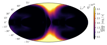
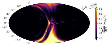
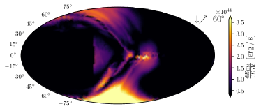
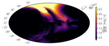
Figure 2: Time-averaged radial Poynting flux ${{\rm d}E_{\rm EM}}/{\left({\rm d}t{\rm d}\Omega\right)}$ projected onto a sphere at $r=370\,\rm km$ from the origin. The time-averaging was done over one flaring period, and includes the removal of the energy flux of the quiescent state of the system. Shown are the models of equal magnetic field strengths, but varying dipole inclinations (A0–A90). The plots adopt a Mollweide projection and are aligned with the orbital rotation axis.

In the following, we will present the results of our numerical investigation of pre-merger flaring in a coalescing binary neutron star system. In particular, we will demonstrate the feasibility of the flaring mechanism for a variety of magnetic field topologies and orbital parameters. In doing so, we will proceed in two steps. First, in Sec.III.1-III.4 we will demonstrate the global dynamics of the flaring process for various binary configurations. We will also show how the emission geometry correlates with the magnetic field topology. In the second part, Sec. III.5, we will estimate the amount of electromagnetic energy emitted and dissipated in this process. This will help to make quantitative predictions about the potential detectability of electromagnetic transients associated with the flaring process.

In all of this work, we consider a series of neutron star binaries at fixed orbital separation $a=52\,\rm$ km, which corresponds to the late inspiral of the binary, i.e. $\lesssim 10$ orbits before merger. This close interaction was identified as the most promising, since the luminosity of the flaring process was shown to scale as $a^{-7/2}$ with the orbital separation $a$ [51]. We further fix the magnetic field strength at the pole of the primary neutron star to $B_{1}=1.9\times 10^{12}\,\rm G$, see Tab. 1.

III.1 Effects of dipole inclination

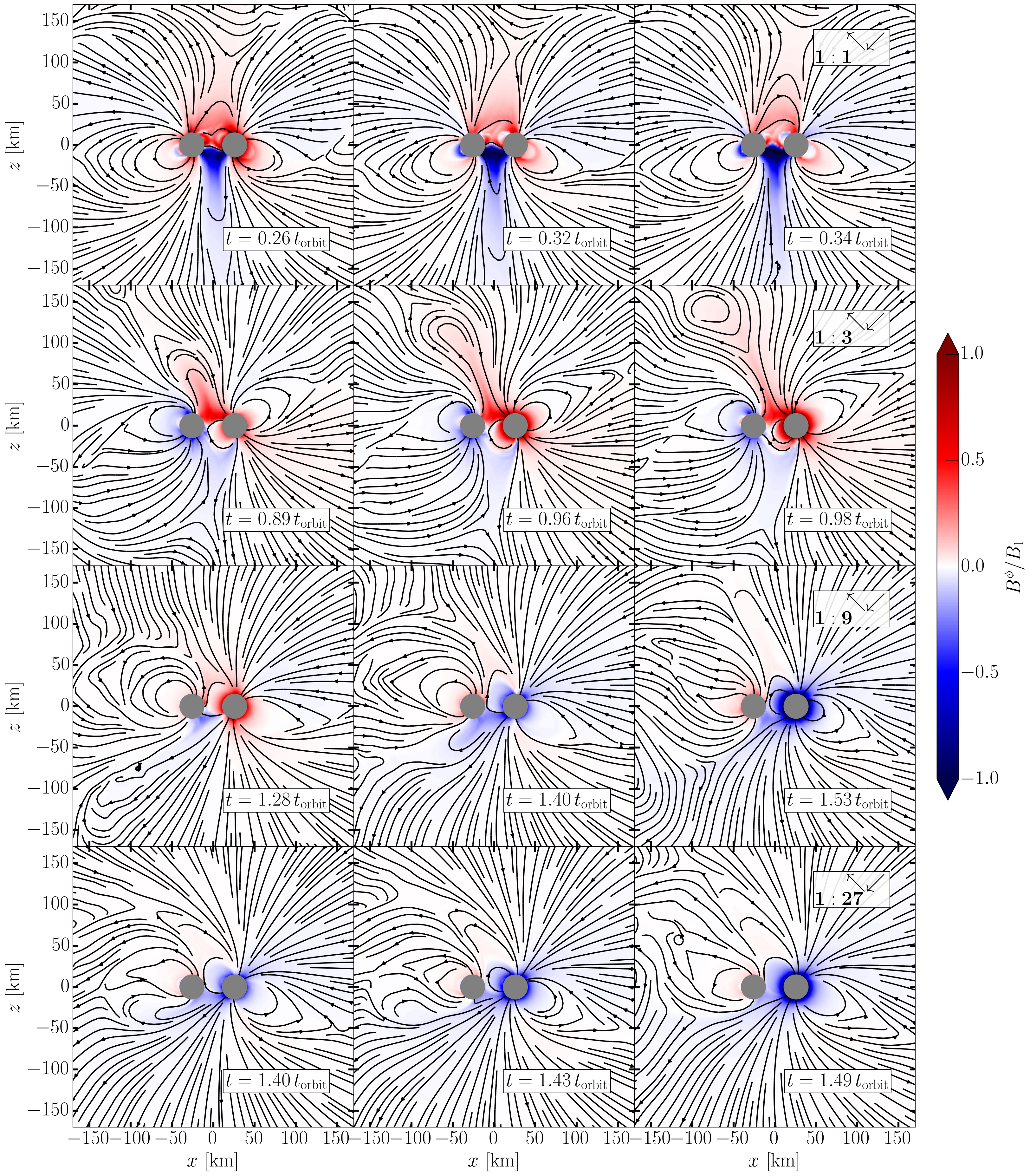
Figure 3: Global flaring dynamics for asymmetric field strengths in a close contact neutron star binary with misaligned dipole magnetic fields. Same as Fig. 1, but for the unequal field strength models (U0–U27).

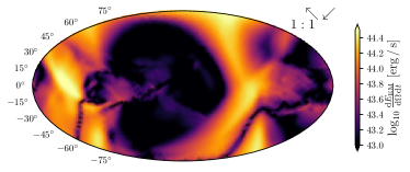
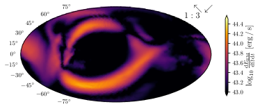
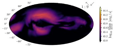
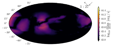
Figure 4: Time-averaged radial Poynting flux $\frac{{\rm d}E_{\rm EM}}{{\rm d}t\,{\rm d}\Omega}$ projected onto a sphere at $r=370\,\rm km$ from the origin. Same as Fig. 2, but for different field strengths on the secondary star (see models U0–U27 in Tab. 1).

In order to better understand the flaring dynamics, we start out by reviewing the flaring mechanism first described in [51]. For this we consider two equally magnetized neutron stars with magnetic moments pointing in opposite directions (model A0), see also the first row of Fig. 1. Since the orbital motion will have reignited the pair-cascade long before the final orbits of the inspiral, the ambient medium is filled with a force-free pair-plasma [27, 28, 29]. As a consequence, the oppositely pointing magnetic field lines can reconnect, and form closed loops (top left panel of Fig. 1). Since all binaries considered here are irrotational and not tidally locked [101], the stars rotate relative to each other when seen in the orbital corotating frame, see also Ref. [53]. The relative rotation of the two stars builds up a twist in the connecting magnetic flux tube, transferring (orbital) rotational energy into the magnetosphere. This twist is mediated by launching Alfven waves along the flux tube [102], which strictly requires the orbital period to be larger than the Alfven wave travel time, hence, demanding that the twisting happens inside the orbital light cylinder with radius $r_{L}=c/\Omega=184\,{\rm{km}}\gg a$ for all models. Once magnetic field lines become more and more twisted, a solar flare like eruption will occur, which features a trailing current sheet that will form between them (top middle panel Fig. 1). As the current sheet become tearing-mode unstable, reconnection will lead to the formation of plasmoids (not shown in Fig. 1) and the disruption of the sheet [51]. This will in turn lead to the detachment of a magnetic bubble (top right panel of Fig. 1) being able to shock the ambient medium further away from the system and potentially lead to the emission of radio emission via a synchrotron maser process [103, 104]. Additionally, the dissipation in the current sheet might lead to X-ray emission [52].
The amount of available magnetic flux that can be twisted and reconnected will depend on the relative inclination of the magnetic fields. To clarify this dependence, we have performed a set of simulations (models A30, A60 and A90) with varying relative inclination, where we have defined $0^{\circ}$ inclination as the case of oppositely aligned magnetic moments. To avoid the issue of relative alignment of the two dipoles, see Sec. III.1, we focus on the scenario where only one of the dipoles is inclined. These cases are shown in the lower three rows of Fig. 1. In all cases, we can see that a sufficient number of magnetic flux tubes is available for twisting. However, the effective twists become weaker for increasing inclinations. For model A90, the twisted flux tube is not in plane and the emission is not symmetric (i.e. along the rotation axis), which differs from model A0, for which no inclination and, thus, symmetry breaking is present. Crucially, the flaring mechanism operates in either case. That is, once an over twisting sets in, reconnection at the base of the loop snaps the field lines, and a detached magnetic bubble is launched from the merger site. This happens even in the case of strong misalignment, where both bubbles and trailing current sheets are present in the northern and southern hemisphere (e.g., bottom right panel of Fig. 1).

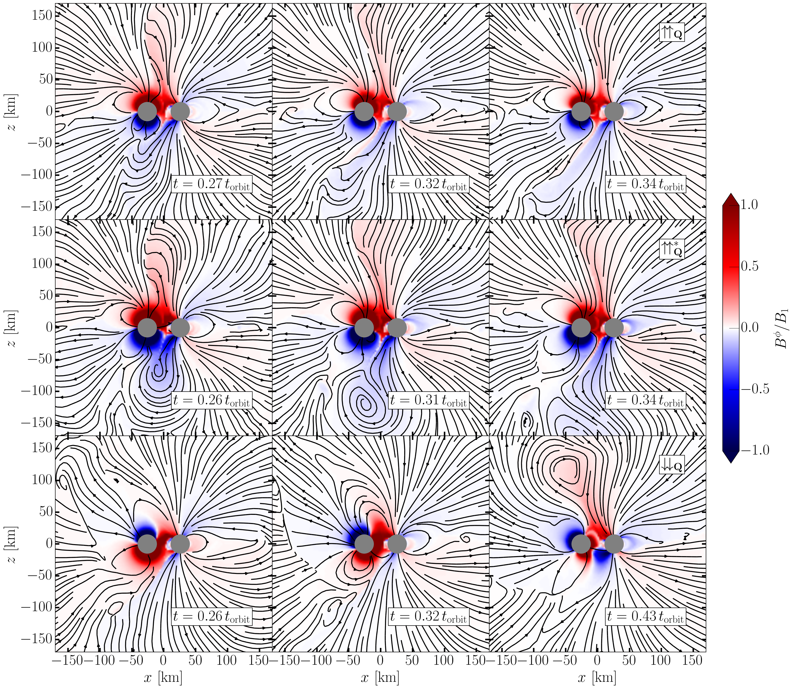
Figure 5: Global flaring dynamics for quadrudipolar magnetic field configurations. Same as Fig. 1 but for models, Q$\uparrow\uparrow$, Q${}^{\ast}\uparrow\uparrow$ and Q$\downarrow\downarrow$.

In order to better quantify the emission geometry of the flares, we study the projection of a single flaring event onto a sphere corotating with the orbital angular velocity $\Omega$. Since we are simulating within the orbital corotating frame, the sphere remains fixed w.r.t. the stars. The sphere is located about $370\,{\rm km}\simeq 7.1a$ from the center-of-mass of the binary. Following our discussion in Sec. III.5.1, we quantify the flare in terms of its Poynting flux $S^{i}_{\rm EM}$, see (17). Instead of showing the spherical projection of the Poynting flux at a fixed time, we isolate a single flare, and then integrate the radial Poynting flux $S^{r}=S^{\mu}_{\rm EM}r^{\nu}g_{\mu\nu}/r$ in time over one flaring episode, where $r^{\nu}$ is spherical radius vector with length $r$. Furthermore, we subtract the time-averaged Poynting flux before and after the flaring event. This way, we can approximately remove the intrinsic Poynting flux due to rotation of the stars in the corotating frame. The resulting distributions are shown in Fig.2. Starting from the fully anti-aligned system (top left), we can see that in this geometry the twisting of the connected flux tube happens roughly in the meridional plane. After the end points of the loop have reconnected, a flare is then launched, propagating entirely in the polar direction, and hence crossing the sphere exactly at the poles. This is the same situation investigated previously in Ref. [51]. With varying inclination, the geometry of the flares becomes more non-axisymmetric. While in the perfectly anti-aligned cases, the same flux is available in both hemispheres and can be equally twisted, this no longer holds for the inclined models. In fact, one can clearly see that the flares emerge from primarily reconnecting magnetic flux in the upper of the lower hemisphere (see e.g., bottom row of Fig. 2). For the $90^{\circ}$ model, A90, the flaring happens exclusively in either hemisphere. Since the flaring is periodic with half the orbital period in this case, the system will be flaring in each hemispheric direction with a full orbital period. Additionally, the flares become more and more axisymmetric, being beamed into the direction of the inclined secondary (left), with the flux going as low as $\theta=60^{\circ}$ latitude, compared to only $\theta=75^{\circ}$ latitude for the anti-aligned $(0^{\circ})$ model. We also point out that the residual Poynting flux on the equatorial plane, $\theta=0^{\circ}$, is a result of imperfect removal of the constant Poynting flux from the rotation of the inclined magnetic field. Therefore, this part is not associated with flaring, and instead does also not overlap with the flare, which propagates predominantly in the polar direction. While on first glance the energy flux of the flare appears comparable in all cases, we will quantify the differences in Sec. III.5.

III.2 Effects of unequal magnetization

Following up on our previous discussion of magnetic field inclination effects in Sec. III.1, we now focus on the general case were the magnetic fields are misaligned and not equal in field strength. We focus on a close binary having two dipolar magnetic moments misaligned by $30^{\circ}$ with their respective stellar spin axis. Different from the previous cases (A0–A90), the secondary has a weaker field strength $B_{2}=B_{1}/3^{n}$ for $n=\left[0,1,2,3\right]$ and a moderate spin of $f_{2}=100\,\rm Hz$. We follow the same logic as in Sec. III.1 and begin by first discussing the global flaring properties shown in Fig. 3, before moving on to describing the emission geometry of the Poynting fluxes in Fig. 4.
We now describe the overall flaring dynamics shown in Fig. 3. Starting with the case of equally strong dipolar fields (top row) we can see that the flaring process proceeds in the same way as for the perfectly anti-aligned fields (top row, Fig. 1). A twist will build up in the common magnetospheres, leading the connected flux tubes to reconnect and flare. Because of the different inclination of both stars the flaring will largely proceed in the polar direction but out of the meridional plane. Once we start to decrease the magnetic field strength of the secondary by a factor three (second row), we can see that the flaring happens in the same way (this time even being more in-plane). However, because of the weaker field on the secondary, the twist will build up closer to its surface, while the emerging loop of field lines bends closer around the secondary star (right column, second row). As the flaring proceeds, we can see that ejected flare is inclined towards the more weakly magnetized secondary (right column).
When decreasing the field strength by a factor nine (third row) this trend easily continues. In fact, the twisted loop is now much closer to the secondary (middle panel), and the twist – expressed in terms of the out-of-plane field $B^{\phi}$ – becomes weaker. The flares are heavily bent towards the secondary. Finally, if we decrease the field strength further (bottom row), flares are still being emitted. However, the twist builds up almost at the surface of the secondary, with the twisted flux tubes protruding far behind the secondary (left panel).

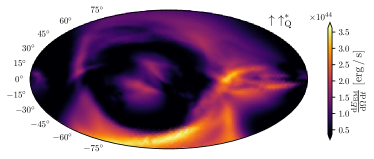
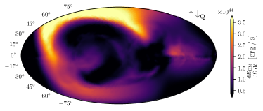
Figure 6: Time-averaged radial Poynting flux ${{\rm d}E_{\rm EM}}/{{\rm d}t}$ projected onto a sphere at $r=370\,\rm km$ from the origin. Same as Fig. 2 but showing models Q${}^{\ast}\uparrow\uparrow$ and Q$\downarrow\downarrow$.

Reconnection then triggers a detachment of the magnetic bubble, with the flare being emitted essentially along the equator (middle and right panels). While flares kept being emitted regardless of the field strength differences, it is apparent that a strong disparity in magnetic field strengths does not only affect the strength of the flare but also the emission geometry.
In order to quantify this dependence further, we now present time-averaged Poynting fluxes of the flares emitted in each system. This is shown in Fig. 4. The overall behavior is very similar to that found for the different inclined models (see Fig. 2). Starting with the equal field strength model (top left), we find that as in the anti-aligned case, two flares are being emitted, one of them in the northern, the other in the southern hemisphere of the binary. Both flares are equal in strength and are propagating mainly along the polar axis. Different from the models presented in Fig. 2, here the flaring is also significantly off-axis at the same time, with the flare covering a large angular space. Even when decreasing the field strength of the secondary by only a factor three (top right), the field strength of the flare decreases. Moreover, the two flares become unequal in strength and extent, with one of them being more strongly beamed towards the secondary. It is important to remember that the flares are being emitted in opposite hemisphere every half orbit because of the relative misalignment of the dipoles. That is, the flaring periodicity is half an orbit ($\approx 2\,\rm ms)$, whereas the periodicity to emit a strong flare into the same hemisphere is a full orbit ($\approx 4\,\rm ms$). When further decreasing the field strength (bottom row), still two flares are being emitted, but especially in the lowest magnetization case U27, the flare is weak compared to the orbital Poynting flux (left of bottom right panel), and becomes confined to the equatorial region. Hence, the flaring mechanism becomes less viable in this case, as spatial coverage and field strength both become much smaller than in the equally magnetized case. We will quantify this behavior further in Sec. III.5.

III.3 Effects of multipolar field structure

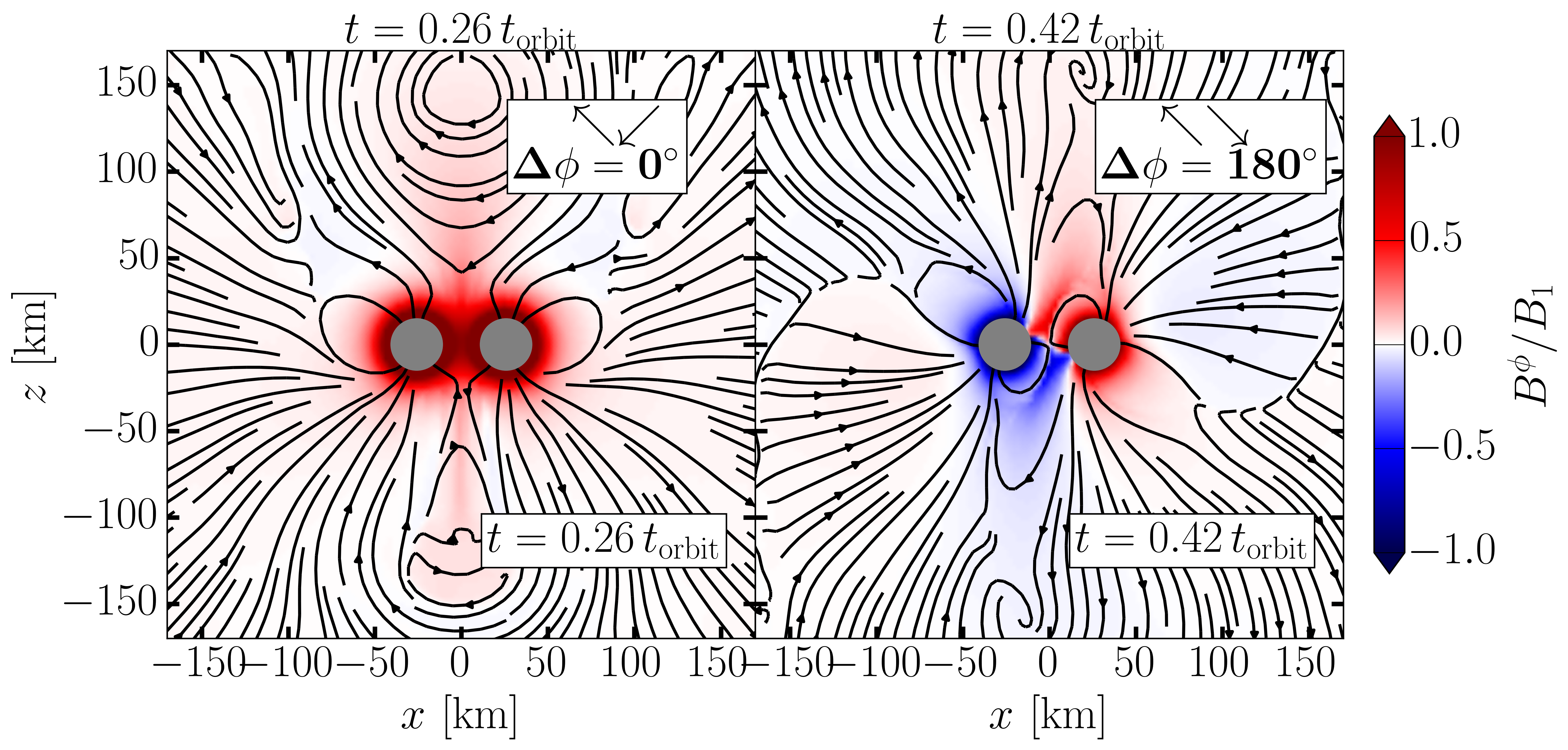
Figure 7: Impact of relative rotation $\Delta\Phi$ of two inclined dipoles (models O0 and O180) on the final flaring state. A detailed description of the quantities shown in this figure is provided in the caption of Fig. 1.

After showing the impact of different magnetic field inclinations and strengths, we want to briefly comment on the effect that different magnetic field topologies can have on the flaring process. While the field on large scales is naturally expected to be dipolar [105], recent observations of PSR J0030+0451 have put forth the possibility of having multipolar field components close to the surface [91]. Since these might be probed in the common magnetosphere close to merger, we choose to include one fiducial model with non-dipolar field geometry. More specifically, we chose a field structure that globally resembles a dipolar field, while locally having an axisymmetric quadrupolar correction [90]. The expression for this field is provided in (32). There, the correction is quantified in terms of a quadrupolar field strength parameter, $\mathcal{Q}_{0}$. In order to investigate its impact, we consider two configuration with $\mathcal{Q}_{0}$, leading either to a small or large quadrupolar correction.
The interesting difference between a dipolar and a quadrupolar field topology lies mainly in the available magnetic field lines that can form closed flux tubes. While two aligned dipoles are not able to form connected flux tubes, the presence of a quadrupolar part supplies additional anti-aligned field lines that can (re-)connect. In other words, flaring in a quadrudipole can either happen via twisting the dipolar part, which is similar to the models considered in Sec. III.1-III.2, or via the quadrupolar part. To this end, we consider three models Q$\uparrow\uparrow$, Q${}^{\ast}\uparrow\uparrow$ and Q$\downarrow\downarrow$ with different alignments and quadrupolar strengths, see Tab. 1 for details. As in Sec. III.1-III.2, we are going to first describe the general flaring dynamics of this configuration and then quantify the amount of energy in the system, that is either dissipated or outgoing in terms of a Poynting flux. We first focus on the aligned configurations, Q$\uparrow\uparrow$, Q${}^{\ast}\uparrow\uparrow$, shown in the top and middle row of Fig. 5, respectively. Looking at the northern hemisphere of these plots, we can see that the aligned magnetic field geometry bars the formation of connected flux tubes. Indeed no significant build-up of out-of-plane magnetic field, $B^{\varphi}$, occurs. Instead, twisting between the dipolar and quadrupolar fields of two two stars in the southern hemisphere, leads to a built-up of twisted field lines (left panels). However, the strength of this twist crucially depends on the relative size of the quadrupolar correction $\mathcal{Q}_{0}$. In fact, for small quadrupolar corrections, Q$\uparrow\uparrow$, the twist can only build up close to the star, as the quadrupolar field lines do not extend close enough to the binary companion. As a result, the energy stored in the twisted flux tube is small, as is the flare. On the other hand, if the correction is significant ( Q${{}^{\ast}}\!\uparrow\uparrow$, middle row), large twists can build up in the quadrupolar field, leading to strong flaring, as in the dipole case. For anti-aligned configurations (bottom row), twists can build up in both hemispheres, leading to the emission of flares from the quadrupolar (left and middle panel) and dipolar sector (right panel). The strength of the quadrupolar flare, in turn, depends on the correction strength $\mathcal{Q}_{0}$.
We provide a more quantitative discussion in Fig. 6, which shows the time averaged Poynting flux during a flaring event projected onto a sphere at a distance of $r=370\,\rm km$ from the origin (see Fig. 2 and Fig. 4). Focusing first on model Q${}^{\ast}\uparrow\uparrow$ (right panel), we can see that two flares are being emitted predominantly in the polar direction. The energy fluxes are overall similar to the other equal field strength models, see Fig. 2. For the misaligned case, Q$\downarrow\downarrow$ (right), a strong flare is emitted, with a corresponding weaker flare in the southern hemisphere. This flare is more inclined towards the secondary, but consistent with the $60^{\circ}$ inclination of the quadrudipolar fields.
Overall, the flaring mechanism does not appear to be affected by the multipolar substructure in the magnetic field. However, the availability of the quadrudipolar field corrections causes additional flares to be emitted. In other words, we would expect substructure in the flaring luminosities, where instead of one flare, there would be secondary smaller flare appearing. We will discuss this point in more detail in Sec. III.5.

III.4 Impact of relative phase difference

For systems not having magnetic moments aligned with the orbital angular momentum another degree of freedom emerges: Relative initial offset of the two dipoles. We investigate the impact of this, by considering two dipoles (models O0 and O180), each of them being inclined by $60^{\circ}$ with respect to the orbital rotation axis. For one of these systems (O180), we include a relative phase difference of $180^{\circ}$ relative to the stellar rotation axis. Put differently, the initial fields are mirror images of each other. Similar to Fig. 1, we report the final flaring state in terms of the out-of-plane magnetic field component $B^{\phi}$ (in orbital cylindrical coordinates) in Fig. 7. We can see that the different relative offset least to different flaring geometries, with the flare launched roughly along the orbital axis (left panel) or completely off-axis (right panel). Also the field strength of the twisted field component gets modified. In fact, the electromagnetic emission for both cases proceeds similarly, that is the flaring geometry results in the same flares, however, their amplitudes are different, as the number of closed field lines available is different in each case. We will discuss this shortly in Sec. III.5 when explicitly quantifying the total amount of electromagnetic energy dissipated in the system.

III.5 Electromagnetic energy budget

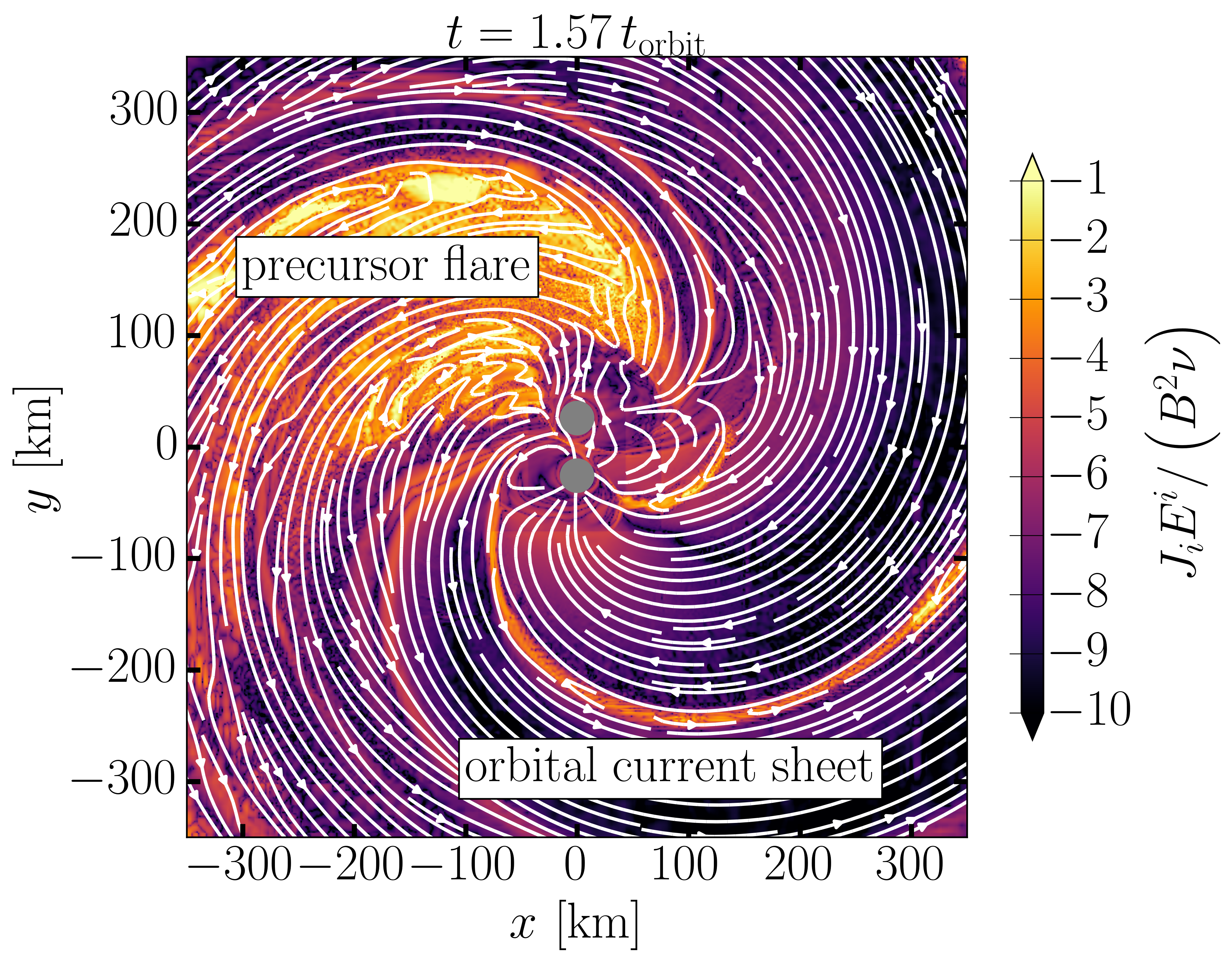
Figure 8: Dissipation rate of electromagnetic energy, $J_{i}E^{i}$, shown in the orbital plane of model A30 during a flaring event. Highlighted are the orbital current sheet (bottom) and the dissipation induced by the precursor flaring event (top). A large part of this is associated with reconnection in trailing current sheet. The magnetic field lines are shown as white lines projected onto the orbital plane. The normalization is set by the magnetic field strength $\sqrt{B^{2}}$ and the dissipation rate $\nu$.

Having established that the precursor flaring mechanism is viable for generic magnetic field topologies and spins in neutron star binaries, we now want to quantitatively describe the amount of energy emission and dissipation in the system. The latter is important for providing quantitative estimates of the amount of energy available to produce observable transients.

The ab-initio modeling of the microphysical processes powering these transients would require accurate knowledge of the dissipation in our simulations, e.g. in terms of the electric field in the reconnecting current sheets, e.g. [106]. However, the intrinsic simplifying limitations of a force-free approach bar us from computing first-principle particle acceleration and dissipation in the system. Yet, we can still provide a meaningful upper bound on the energy available for such processes by computing the amount of energy, which is (numerically) dissipated in the calculations. Future work will be necessary to augment force-free-type simulations with meaningful closure prescriptions for electromagnetic energy dissipation [107].

III.5.1 Quantifying dissipation

Within our simulation we can easily quantify the total amount of electromagnetic energy $E_{\rm EM}^{\mathcal{V}}$ within a volume $\mathcal{V}$ by spatially integrating Eq. (16),

$$E_{\rm EM}^{\mathcal{V}}=\int_{\mathcal{V}}\rho_{\rm EM}\,{\rm d}^{3}x\,,$$ (35)

and the electromagnetic energy flux $\mathcal{S}^{\mathcal{V}}_{\rm EM}$ through the boundary $\partial\mathcal{V}$ of said volume $\mathcal{V}$,

$$\mathcal{S}_{\rm EM}^{\mathcal{V}}=\oint_{\partial\mathcal{V}}\left(S_{\rm EM}\right)_{i}{\rm d}\Sigma^{i}\,,$$ (36)

where ${\rm d}\Sigma^{i}$ is the outwards-pointing surface element.

In our simulations, dissipation will occur mainly in two places. The first one is associated with the (inspiraling) motion of the stars. Just as for an isolated rotating pulsar, the plasma surrounding it can only co-rotate up until the light cylinder. This is the distance from the rotation axis, beyond which the corotational velocity $v=\Omega\varpi$ would exceed the speed of light, i.e. $\varpi_{\rm LC}=c/\Omega$. Beyond this point, the field lines will have to open up, separating them by a strong current sheet [87]. Since current sheets are the sole point of magnetic dissipation, the continued presence of the orbital current sheet will cause a constant amount of net dissipation, see e.g. [54]. This can be seen in Fig. 8, which shows the local energy dissipation rate $J_{i}E^{i}$ in the orbital plane for model A30. For reference, we estimate that the orbital sheet is locally dissipating $\simeq 10^{29}\,\left(B/10^{12}\rm G\right)^{2}\,\rm erg/\left(s\,cm^{3}\right)$. During a flaring event (top of Fig. 8), the trailing current sheet of the flare and its interaction with the orbital current sheet, cause additional dissipation (in the trailing current sheet). In this specific model, A30, locally up to 100-times larger than in the orbital current sheet. We emphasize that in the absence of a more realistic Ohm’s law prescription [107] the precise numbers should be considered approximate.

In order to quantify the the amount of dissipation, we introduce an associated luminosity $\mathcal{L}_{\rm diss}^{\mathcal{V}}$ in a volume $\mathcal{V}$, in analogy with the electromagnetic energy $E_{\rm EM}^{\mathcal{V}}$ contained in that volume. From Eq. (19) we find that,

$$\mathcal{L}_{\rm diss}^{\mathcal{V}}:= \int_{\mathcal{V}}J_{i}E^{i}{\rm d}^{3}x$$

$$= \,\partial_{t}E_{\rm EM}^{\mathcal{V}}+\mathcal{S}_{\rm EM}^{\mathcal{V}}\,.$$ (37)

Hence, we can quantify energy dissipation (which physically occurs exclusively in current sheets) using the non-conservation of electromagnetic energy. While it would also be possible to directly compute the dissipation rate, i.e. $J_{i}E^{i}$, from the electric current $J_{\mu}$, the implicit numerical computation of $J_{\mu}$ based on local violations of the force-free conditions(24) makes this rather impractical. In the rest of this paper, we will exclusively adopt spherical volumes $\mathcal{V}$ with radii $r=[r_{\rm in};r_{\rm out}]$, centered on the center of mass of the binary. Since rotation of the two neutron stars is enforced via a boundary condition, there is a net injection of energy from the surface of the two stars into the computational domain. Therefore, we need to ensure that this artificial energy injection rate is not included when evaluating (37). This can be done by choosing $r_{\rm in}>a+r_{\rm NS}$, where $r_{\rm NS}$ is the radius of the neutron star. In this way, the dissipation rate $\mathcal{L}_{\rm diss}$ is only computed between two spherical shells at $r_{\rm in}$ and $r_{\rm out}$. Using the definitions above, we may rewrite (37) as

$$\mathcal{L}_{\rm diss}=\mathcal{S}_{\rm EM}^{r_{\rm out}}-\mathcal{S}_{\rm EM}^{r_{\rm in}}+\frac{{\rm d}}{{\rm d}t}\left(E_{\rm EM}^{r_{\rm out}}-E_{\rm EM}^{r_{\rm in}}\right)\,.$$ (38)

For the remainder of this work we choose $r_{\rm in}=2.3\,a$ and $r_{\rm out}=12.3\,a$, where $a$ is the orbital separation, see Tab. 1. We have ensured that the flaring happens both inside the shell and that the choice of outer radius has negligible effect on the extraction of the Poynting flux and energy dissipation rate.

III.5.2 Energy budget of a precursor flare

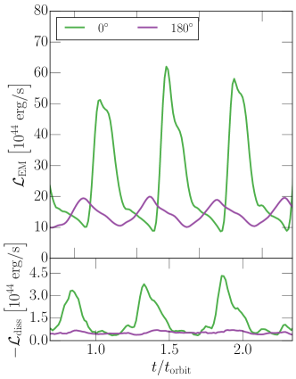
Figure 9: Electromagnetic luminosity $\mathcal{L}_{\rm EM}$ of the precursor flares for different relative rotation $\Delta\Phi$ of the two dipoles (models O0 and O180), in an equally magnetized neutron star binary. (Top) Positive values refer to outgoing Poynting fluxes computed on a sphere with radius $r=12.3a$, where $a$ denotes the orbital separation. (Bottom) The dissipative luminosity $\mathcal{L}_{\rm diss}$ refers to the energy dissipated in current sheets within a spherical shell between $r_{\rm in}=2.3\,a$ and $r_{\rm out}=12.3\,a$. The times $t$ are expressed relative to the orbital period $t_{\rm orbit}$.

Following our discussion of how to quantify dissipation in current sheets, Sec. III.5.1, we now compute the energy budget of the flare in terms of dissipated energy and outgoing Poynting flux. Before presenting a comparison of the flares obtained for different magnetic field inclinations (Sec. III.1), magnetizations (Sec. III.2) and topologies (Sec. III.3) , we illustrate the analysis using models O0 and O180 presented in Sec. III.4. The resulting luminosities are shown in Fig. 9. In both cases we find a periodic signal in the Poynting flux (top curves). The periodicity of the flares corresponds to half of the orbital time scale, as expected. The initial offset of the dipoles translates to a quarter orbital time shift in the flares, the strength of which changes by about a factor three between the two configurations. We point out that when (gravitational wave) radiation backreaction was included, the strength of the Poynting flux would increase with time, whereas the period would shrink, as the two stars inspiral. Looking at the dissipation (bottom panel), we find clear periodic dissipation associated with the flares in the O0 model with $0^{\circ}$ relative phase shift between the dipoles. In the O180 model, however, the dissipation in trailing current sheet is strongly suppressed. Indeed, the almost constant level of dissipation coincides with the lower dissipation limit of the O0 model. This is a strong indication that dissipation is dominated by the contribution from the orbital current sheet that is constantly sourced by the orbital motion of the stars, see Fig. 8.
While the emission associated with the direct emission of a magnetic bubble in the flare will always be present, transients associated with dissipation in the trailing current sheet [108], might strongly depend on the relative phase offsets of the two magnetic fields. For surface magnetic field strengths of $\simeq 10^{12}\,\rm G$, the luminosities of are always of the order $10^{44}-10^{45}\rm erg/s$ with dissipation being at least an order of magnitude smaller. This is consistent with our earlier findings of the flaring process [51].

III.5.3 Dependence on magnetic field topology

Following our detailed description of the flaring process and its energetics, we are finally in a position to compare the energetics of the different models considered in this work. More specifically, we are interested in understanding how the total luminosity of the flare and the dissipation it induces scale with the inclination of the magnetic field, and the field strength of its companion. To this end, we show the energetics in Fig. 10, in a similar fashion to Fig. 9. Starting with the case of relative magnetic field inclination but equal magnetic moments, models A0–A90, we find that the luminosity of the flares vary within a factor $L_{\rm EM}/L_{\rm EM}^{0^{\circ}}\simeq 2$ relative to the aligned system. Looking at the lower left panel of Fig. 10, we find that the dissipated energy rate is about a factor $5$ smaller in all cases. Despite the clear dependence of the luminosity of the flare on the relative size of the magnetic moments of the two neutron stars, the dissipation rate in the trailing current sheet is roughly the same in either case. This is similar in behavior and magnitude to the cases with different inclination angle. This strongly indicates the the energy dissipated in current sheet might be largely independent of the choice of magnetic field topology. For the case of the quadrudipole topology (right panels) the situation is similar. Small variations in the energy dissipation rate exist, but for equal magnetization the overall dissipation rate is roughly the same. The Poynting fluxes of all three cases show mild variations, with repeated flaring activity. The strength of the flares directly correlates with the amount of flux tubes available for the flaring process. Indeed, for the smallest quadrudipole configuration in the aligned cases ($\uparrow\uparrow_{Q}$) only a tiny fraction of field lines from the quadrupolar part can be twisted, see also Fig. 5. This increases with stronger quadrupole component ($\uparrow\uparrow_{Q}$). Indeed, for the anti-aligned cases both the quadrupolar and dipolar part can be twisted. This results in a double peak sub-structure, with the strong flares corresponding to the dipolar, the weaker once to the quadrupolar part. The overall luminosity only varies within a factor 2 between the different configurations.

This leads us to conclude that both the dissipation, as well as the flaring luminosities are largely invariant under changes of the magnetic field topology. Flaring will only start to cease if the system becomes very unequally magnetized, e.g. for model U27.

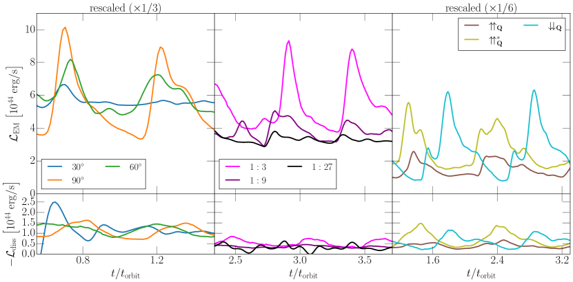
Figure 10: Average Poynting fluxes for different inclinations (left panel), magnetization ratios (middle panel) and quadrudipolar field configuration (right panel). See caption of Fig. 9 for a description of the quantities shown.

III.5.4 How many flares do we expect to be observable?

Now that we have quantified the energetics of the flaring process, we want to estimate how many flares we would expect to be in principle observable. While a detailed discussion of the microphysical emission process is beyond the scope of this paper and will be addressed in a forthcoming work, we can already place limits based on the total electromagnetic luminosity available in the process. This will provide an estimate for the upper bound for the available electromagnetic energy radiated per flaring event. We will separately consider radio and X-ray emission.
To this end we will make the following assumptions. First, for slowly rotating or irrotational systems, a flare will be launched after a $180^{\circ}$ twist. This will happen roughly twice per orbital period. The exact expression for arbitrary binary configurations can be found in Ref. [53]. We recall that that the orbital frequency $f$ and the frequency of the gravitational wave signal $f_{\rm GW}$ are related by, $f_{\rm GW}=2f$. Hence, the number of gravitational wave cycles and of flares coincides, and we can write

$$N_{\rm flares}=\int f_{\rm GW}{\rm d}t=\int_{f_{\rm min}}^{f_{\rm max}}\frac{\dot{f}_{\rm GW}}{f_{\rm GW}}{\rm d}f_{\rm GW}\,,$$ (39)

where $f_{\rm min}$ and $f_{\rm max}$ are initial and final frequency bounding the interval of the inspiral with $N_{\rm flares}$ gravitational-wave cycles. Assuming that $f_{\rm max}\gg f_{\rm min}$, one can integrate (39) to yield [109],

$$N_{\rm flares}=\frac{1}{32\pi^{8/3}}\left(\frac{G\mathcal{M}}{c^{3}}f_{\rm min}\right)^{-5/3}\,.$$ (40)

Here, we have introduced Newton’s constant $G$, the speed of light $c$ and the chirp mass $\mathcal{M}=\left[q/\left(1+q\right)^{2}\right]^{3/5}M$, which is determined by the binary masses $m_{1}$ and $m_{2}$ in the form of the total mass $M=m_{1}+m_{2}$ and the mass ratio $q=m_{2}/m_{1}$.

The initial frequency $f_{\rm min}$ is determined by the time, when the flaring luminosity becomes large enough to (in principle) be observable. In good agreement with the present simulations, we previously found that [51],

$$\mathcal{L}_{\rm EM}={\mathcal{L}}_{0}\left(\frac{a_{0}}{a}\right)^{7/2}\,,$$ (41)

where $a_{0}=45\,\rm km$ and

$$\mathcal{L}_{0} =7\times 10^{44}\,\sigma\left(\frac{B_{1}}{10^{12}\,\rm G}\right)^{2}\,,\rm erg/s\,,$$ (42)

for the luminosity of the expanding magnetic bubble, for which the efficiency $\sigma=1$. Here, we have introduced the efficiency $\sigma=0.1$ for X-rays associated with the dissipation in the current sheet, and $\sigma=10^{-5}-10^{-3}$ for radio transients directly associated with the outgoing magnetic bubble. This is true for both the synchrotron maser mechanism at the shock launched by the bubble in the binary wind [110, 52], as well as the emission from plasmoid mergers [111, 108] expected from the collision of the flaring bubble and the magnetospheric current sheet [112]. Other characteristics of the observed signal, such as characteristic frequencies and burst duration, will be studied in a forthcoming work.

From Kepler’s law, we obtain $16\pi^{2}f_{\rm GW}^{2}=GM/\varpi^{3}$. Hence we can relate,

$$f_{\rm min}=\frac{1}{16\pi^{2}}\left(G\mathcal{M}\left[\frac{q}{\left(1+q\right)^{2}}\right]^{3/5}\right)^{1/2}\varpi_{0}^{-3/2}{\mathcal{L}}_{0}^{-3/7}{\mathcal{L}}_{\rm EM}^{3/7}\,.$$ (43)

Combining (43) with (40), we obtain the final scaling

$$N_{\rm flares}=\frac{\left(8\pi\right)^{2/3}}{2^{1/3}}\varpi_{0}^{5/2}\mathcal{L}_{0}^{5/7}\,\left[\frac{\left(1+q\right)^{2}}{q}\right]^{1/2}$$

$$\phantom{N_{\rm flares}=\frac{\left(8\pi\right)^{2/3}}{2^{1/3}}\varpi_{0}^{5/2}\mathcal{L}_{0}^{5/7}\,}\left(\frac{G^{2}\mathcal{M}^{2}}{c^{3}}\right)^{-5/3}\mathcal{L}_{\rm min}^{-5/7}\,,$$ (44)

where $\mathcal{L}_{\rm min}$ is the minimum luminosity required for a detection. Assuming a near-equal mass binary, $q\approx 1$, with canonical neutron star masses $m_{1}=m_{2}=1.4\,M_{\odot}$, we find

$$\phantom{N_{\rm flares}}\simeq 17\left(\frac{B}{10^{11}\,\rm G}\right)^{10/7}\,\left(\frac{1.2M_{\odot}}{\mathcal{M}}\right)^{5/2}\, \left(\frac{10^{42}\,\rm erg/s}{\mathcal{L}_{\rm min}}\right)^{5/7}$$

$$\left(\frac{\sigma}{10^{-4}}\right)^{5/7}\,.$$ (45)

We can see that the number of potentially observable flares will strongly depend on the magnetic field strength and the emission mechanism. More specifically (40) implies, that for magnetic field strengths $\ll 10^{11}\,\rm G$ no flares will be observable. Effects such as unequal magnetization would further decrease the number of flares, as the luminosity can be suppressed by a factor of a few, see Fig. 10. Furthermore, the above estimate does not account for anisotropies in the emission, e.g. beaming effects. This would raise the required luminosity $\mathcal{L}_{\rm min}$ further suppressing the number of potentially observable flares.

IV Conclusions

In this work, we have investigated the impact of different magnetic field topologies on the precursor flaring mechanism in coalescing neutron star binaries [51]. The interaction of oppositely directed magnetic field configurations in neutron star binaries can lead to the built-up of twists in the common magnetosphere, that will ultimately culminate in the release of a powerful electromagnetic flare, not unlike in a coronal-mass ejection event in the Sun[113].

Focusing on different magnetic field topologies, we have investigated the viability of producing precursor flares in the late inspiral of neutron star binaries. More specifically, we have presented a new set of 13 simulations investigating different magnetic field inclinations, magnetization ratios and quadrudipolar field topologies. One of our main findings is, that the emission of flares will always happen unless one of the two neutron star is significantly less magnetized than the other. In particular, we find a strong suppression of the luminosity of a flare of the field strength differ by ratios much greater than 1:10. Furthermore, we find that the inclusion of higher order multipolar field structure leads to secondary flaring events, when, e.g., the quadrupolar part gets twisted and flares in addition to the twist on the dipolar part. While the production mechanism of flares itself is interesting, their interaction with the surrounding medium might lead to the production of radio transients (e.g., [45]). We have also quantified the amount of dissipation induced by the presence of the flare. In an earlier work [51], we had shown that the trailing current sheets in this process lead to an order-of-magnitude lower luminosity, that is able to power (largely) X-ray transients [52]. Interestingly, we find that the amount of dissipation is largely independent of the flaring geometry. We do find (sometimes small) periodic enhancement in the energy dissipation rate corresponding with individual flaring events. Yet, the amount of dissipation varies at most by a factor of a few compared to the dissipation in the orbital current sheet. We remark, that if the field strength in the flare becomes too weak, i.e $B_{2}\ll 10^{-2}B_{1}$, dissipation will be dominated completely by that of the orbital current sheet.

While our results strongly hint at the presence of electromagnetic flares in the late inspiral of neutron star binaries, we caution that these systems contain inherent uncertainties. Firstly, our study assumes the presence of a force-free pair-plasma in the common magnetosphere [81]. While this might be a reasonable assumption in the late stage of the binary, where the orbital motion can induce strong electric fields [28, 29], it will likely require the presence of sufficiently large magnetic fields [114]. Finally, systems with fully aligned magnetic moments (and only dipole fields) will also not be able to sustain any flaring activity.

Apart from those concerns, our parameter coverage is by no means exhaustive. Although we have only focused on a single orbital separation representative of the late inspiral, we have shown earlier, that the flaring strength strongly correlates with the orbital separation [51]. However, changes in the separation will only affect the orbital velocity and, hence, for most realistic binaries with vanishing stellar spins [101], only the periodicity of the flares. On the other hand, extreme spins might leave strong imprints on the post-merger dynamics (e.g., [115, 116, 117, 118, 119, 120]) and life-time of the system [121, 120]. In terms of the precursor flaring mechanism they would largely affect the periodicity, since the effective rotation frequency in the corotating frame will be $\Omega-\omega$ [49], see also [53] for a complete discussion and more detailed expression for general spins and magnetic field alignments. We note that in the absence of tidal locking [101], the stars are always expected to have an effective twist rate relative to the orbital motion. We intend to provide such a thorough investigation of spin effects in a future study.

Finally, the modeling of the plasma physics in this work can, at best, be considered rudimentary. Meaningful simulations require the use of more accurate Ohm’s law closures for the electric field [122]. Future work using novel approaches to relativistic two-fluid systems will be required to improve the global modeling of these transient phenomena [107].

References

- Abbott et al. [2016a] B. P. Abbott et al. (LIGO Scientific, Virgo), Observation of Gravitational Waves from a Binary Black Hole Merger, Phys. Rev. Lett. 116, 061102 (2016a), arXiv:1602.03837 [gr-qc] .
- Abbott et al. [2016b] B. P. Abbott et al. (LIGO Scientific, Virgo), GW151226: Observation of Gravitational Waves from a 22-Solar-Mass Binary Black Hole Coalescence, Phys. Rev. Lett. 116, 241103 (2016b), arXiv:1606.04855 [gr-qc] .
- Abbott et al. [2016c] B. P. Abbott et al. (LIGO Scientific, Virgo), Binary Black Hole Mergers in the first Advanced LIGO Observing Run, Phys. Rev. X 6, 041015 (2016c), [Erratum: Phys.Rev.X 8, 039903 (2018)], arXiv:1606.04856 [gr-qc] .
- Abbott et al. [2017a] B. P. Abbott et al. (LIGO Scientific, VIRGO), GW170104: Observation of a 50-Solar-Mass Binary Black Hole Coalescence at Redshift 0.2, Phys. Rev. Lett. 118, 221101 (2017a), [Erratum: Phys.Rev.Lett. 121, 129901 (2018)], arXiv:1706.01812 [gr-qc] .
- Abbott et al. [2017b] B. P. Abbott et al. (LIGO Scientific, Virgo), GW170814: A Three-Detector Observation of Gravitational Waves from a Binary Black Hole Coalescence, Phys. Rev. Lett. 119, 141101 (2017b), arXiv:1709.09660 [gr-qc] .
- Abbott et al. [2019] B. P. Abbott et al. (LIGO Scientific, Virgo), GWTC-1: A Gravitational-Wave Transient Catalog of Compact Binary Mergers Observed by LIGO and Virgo during the First and Second Observing Runs, Phys. Rev. X 9, 031040 (2019), arXiv:1811.12907 [astro-ph.HE] .
- Abbott et al. [2020a] R. Abbott et al. (LIGO Scientific, Virgo), GW190521: A Binary Black Hole Merger with a Total Mass of , Phys. Rev. Lett. 125, 101102 (2020a), arXiv:2009.01075 [gr-qc] .
- Abbott et al. [2021a] R. Abbott et al. (LIGO Scientific, Virgo), GWTC-2: Compact Binary Coalescences Observed by LIGO and Virgo During the First Half of the Third Observing Run, Phys. Rev. X 11, 021053 (2021a), arXiv:2010.14527 [gr-qc] .
- Abbott et al. [2020b] R. Abbott et al. (LIGO Scientific, Virgo), Properties and Astrophysical Implications of the 150 M⊙ Binary Black Hole Merger GW190521, Astrophys. J. Lett. 900, L13 (2020b), arXiv:2009.01190 [astro-ph.HE] .
- Abbott et al. [2020c] R. Abbott et al. (LIGO Scientific, Virgo), GW190412: Observation of a Binary-Black-Hole Coalescence with Asymmetric Masses, Phys. Rev. D 102, 043015 (2020c), arXiv:2004.08342 [astro-ph.HE] .
- Abbott et al. [2020d] R. Abbott et al. (LIGO Scientific, Virgo), GW190814: Gravitational Waves from the Coalescence of a 23 Solar Mass Black Hole with a 2.6 Solar Mass Compact Object, Astrophys. J. Lett. 896, L44 (2020d), arXiv:2006.12611 [astro-ph.HE] .
- Abbott et al. [2021b] R. Abbott et al. (LIGO Scientific, VIRGO, KAGRA), GWTC-3: Compact Binary Coalescences Observed by LIGO and Virgo During the Second Part of the Third Observing Run, (2021b), arXiv:2111.03606 [gr-qc] .
- Venumadhav et al. [2019] T. Venumadhav, B. Zackay, J. Roulet, L. Dai, and M. Zaldarriaga, New search pipeline for compact binary mergers: Results for binary black holes in the first observing run of Advanced LIGO, Phys. Rev. D 100, 023011 (2019), arXiv:1902.10341 [astro-ph.IM] .
- Zackay et al. [2019] B. Zackay, T. Venumadhav, L. Dai, J. Roulet, and M. Zaldarriaga, Highly spinning and aligned binary black hole merger in the Advanced LIGO first observing run, Phys. Rev. D 100, 023007 (2019), arXiv:1902.10331 [astro-ph.HE] .
- Olsen et al. [2022] S. Olsen, T. Venumadhav, J. Mushkin, J. Roulet, B. Zackay, and M. Zaldarriaga, New binary black hole mergers in the LIGO–Virgo O3a data, (2022), arXiv:2201.02252 [astro-ph.HE] .
- Abbott et al. [2017c] B. P. Abbott et al. (LIGO Scientific, Virgo), GW170817: Observation of Gravitational Waves from a Binary Neutron Star Inspiral, Phys. Rev. Lett. 119, 161101 (2017c), arXiv:1710.05832 [gr-qc] .
- Abbott et al. [2020e] B. P. Abbott et al. (LIGO Scientific, Virgo), GW190425: Observation of a Compact Binary Coalescence with Total Mass , Astrophys. J. Lett. 892, L3 (2020e), arXiv:2001.01761 [astro-ph.HE] .
- Abbott et al. [2021c] R. Abbott et al. (LIGO Scientific, KAGRA, VIRGO), Observation of Gravitational Waves from Two Neutron Star–Black Hole Coalescences, Astrophys. J. Lett. 915, L5 (2021c), arXiv:2106.15163 [astro-ph.HE] .
- Abbott et al. [2017d] B. P. Abbott et al. (LIGO Scientific, Virgo, Fermi GBM, INTEGRAL, IceCube, AstroSat Cadmium Zinc Telluride Imager Team, IPN, Insight-Hxmt, ANTARES, Swift, AGILE Team, 1M2H Team, Dark Energy Camera GW-EM, DES, DLT40, GRAWITA, Fermi-LAT, ATCA, ASKAP, Las Cumbres Observatory Group, OzGrav, DWF (Deeper Wider Faster Program), AST3, CAASTRO, VINROUGE, MASTER, J-GEM, GROWTH, JAGWAR, CaltechNRAO, TTU-NRAO, NuSTAR, Pan-STARRS, MAXI Team, TZAC Consortium, KU, Nordic Optical Telescope, ePESSTO, GROND, Texas Tech University, SALT Group, TOROS, BOOTES, MWA, CALET, IKI-GW Follow-up, H.E.S.S., LOFAR, LWA, HAWC, Pierre Auger, ALMA, Euro VLBI Team, Pi of Sky, Chandra Team at McGill University, DFN, ATLAS Telescopes, High Time Resolution Universe Survey, RIMAS, RATIR, SKA South Africa/MeerKAT), Multi-messenger Observations of a Binary Neutron Star Merger, Astrophys. J. Lett. 848, L12 (2017d), arXiv:1710.05833 [astro-ph.HE] .
- Mooley et al. [2018] K. P. Mooley et al., A mildly relativistic wide-angle outflow in the neutron star merger GW170817, Nature 554, 207 (2018), arXiv:1711.11573 [astro-ph.HE] .
- Kasliwal et al. [2017] M. M. Kasliwal et al., Illuminating Gravitational Waves: A Concordant Picture of Photons from a Neutron Star Merger, Science 358, 1559 (2017), arXiv:1710.05436 [astro-ph.HE] .
- Hallinan et al. [2017] G. Hallinan et al., A Radio Counterpart to a Neutron Star Merger, Science 358, 1579 (2017), arXiv:1710.05435 [astro-ph.HE] .
- Cowperthwaite et al. [2017] P. S. Cowperthwaite et al., The Electromagnetic Counterpart of the Binary Neutron Star Merger LIGO/Virgo GW170817. II. UV, Optical, and Near-infrared Light Curves and Comparison to Kilonova Models, Astrophys. J. Lett. 848, L17 (2017), arXiv:1710.05840 [astro-ph.HE] .
- Drout et al. [2017] M. R. Drout et al., Light Curves of the Neutron Star Merger GW170817/SSS17a: Implications for R-Process Nucleosynthesis, Science 358, 1570 (2017), arXiv:1710.05443 [astro-ph.HE] .
- Chornock et al. [2017] R. Chornock et al., The Electromagnetic Counterpart of the Binary Neutron Star Merger LIGO/VIRGO GW170817. IV. Detection of Near-infrared Signatures of r-process Nucleosynthesis with Gemini-South, Astrophys. J. Lett. 848, L19 (2017), arXiv:1710.05454 [astro-ph.HE] .
- Villar et al. [2017] V. A. Villar et al., The Combined Ultraviolet, Optical, and Near-Infrared Light Curves of the Kilonova Associated with the Binary Neutron Star Merger GW170817: Unified Data Set, Analytic Models, and Physical Implications, Astrophys. J. Lett. 851, L21 (2017), arXiv:1710.11576 [astro-ph.HE] .
- Hansen and Lyutikov [2001] B. M. S. Hansen and M. Lyutikov, Radio and x-ray signatures of merging neutron stars, Mon. Not. Roy. Astron. Soc. 322, 695 (2001), arXiv:astro-ph/0003218 .
- Lyutikov [2019] M. Lyutikov, Electrodynamics of binary neutron star mergers, Mon. Not. Roy. Astron. Soc. 483, 2766 (2019), arXiv:1809.10478 [astro-ph.HE] .
- Wada et al. [2020] T. Wada, M. Shibata, and K. Ioka, Analytic properties of the electromagnetic field of binary compact stars and electromagnetic precursors to gravitational waves, PTEP 2020, 103E01 (2020), arXiv:2008.04661 [astro-ph.HE] .
- Callister et al. [2019] T. A. Callister, M. M. Anderson, G. Hallinan, L. R. D’addario, J. Dowell, N. E. Kassim, T. J. W. Lazio, D. C. Price, and F. K. Schinzel, A First Search for Prompt Radio Emission from a Gravitational-Wave Event, Astrophys. J. Lett. 877, L39 (2019), arXiv:1903.06786 [astro-ph.HE] .
- McWilliams and Levin [2011] S. T. McWilliams and J. Levin, Electromagnetic extraction of energy from black hole-neutron star binaries, Astrophys. J. 742, 90 (2011), arXiv:1101.1969 [astro-ph.HE] .
- D’Orazio and Levin [2013] D. J. D’Orazio and J. Levin, Big Black Hole, Little Neutron Star: Magnetic Dipole Fields in the Rindler Spacetime, Phys. Rev. D 88, 064059 (2013), arXiv:1302.3885 [astro-ph.HE] .
- Mingarelli et al. [2015] C. M. F. Mingarelli, J. Levin, and T. J. W. Lazio, Fast Radio Bursts and Radio Transients from Black Hole Batteries, Astrophys. J. Lett. 814, L20 (2015), arXiv:1511.02870 [astro-ph.HE] .
- D’Orazio et al. [2016] D. J. D’Orazio, J. Levin, N. W. Murray, and L. Price, Bright transients from strongly-magnetized neutron star-black hole mergers, Phys. Rev. D 94, 023001 (2016), arXiv:1601.00017 [astro-ph.HE] .
- Bransgrove et al. [2021] A. Bransgrove, B. Ripperda, and A. Philippov, Magnetic Hair and Reconnection in Black Hole Magnetospheres, Phys. Rev. Lett. 127, 055101 (2021), arXiv:2109.14620 [astro-ph.HE] .
- Wang et al. [2016] J.-S. Wang, Y.-P. Yang, X.-F. Wu, Z.-G. Dai, and F.-Y. Wang, Fast Radio Bursts from the Inspiral of Double Neutron Stars, Astrophys. J. Lett. 822, L7 (2016), arXiv:1603.02014 [astro-ph.HE] .
- James et al. [2019] C. W. James, G. E. Anderson, L. Wen, J. Bosveld, Q. Chu, M. Kovalam, T. J. Slaven-Blair, and A. Williams, Using negative-latency gravitational wave alerts to detect prompt radio bursts from binary neutron star mergers with the Murchison Widefield Array, Mon. Not. Roy. Astron. Soc. 489, L75 (2019), arXiv:1908.08688 [astro-ph.HE] .
- Sachdev et al. [2020] S. Sachdev et al., An Early-warning System for Electromagnetic Follow-up of Gravitational-wave Events, Astrophys. J. Lett. 905, L25 (2020), arXiv:2008.04288 [astro-ph.HE] .
- Yu et al. [2021] H. Yu, R. X. Adhikari, R. Magee, S. Sachdev, and Y. Chen, Early warning of coalescing neutron-star and neutron-star-black-hole binaries from the nonstationary noise background using neural networks, Phys. Rev. D 104, 062004 (2021), arXiv:2104.09438 [gr-qc] .
- Wang et al. [2020] Z. Wang, T. Murphy, D. L. Kaplan, K. W. Bannister, and D. Dobie, The capability of the Australian Square Kilometre Array Pathfinder to detect prompt radio bursts from neutron star mergers, Publ. Astron. Soc. Austral. 37, e051 (2020), arXiv:2010.09949 [astro-ph.IM] .
- Broderick et al. [2020] J. W. Broderick et al., LOFAR 144-MHz follow-up observations of GW170817, Mon. Not. Roy. Astron. Soc. 494, 5110 (2020), arXiv:2004.01726 [astro-ph.HE] .
- Stachie et al. [2021a] C. Stachie et al., Predicting electromagnetic counterparts using low-latency gravitational-wave data products, Mon. Not. Roy. Astron. Soc. 505, 4235 (2021a), arXiv:2103.01733 [astro-ph.HE] .
- Stachie et al. [2021b] C. Stachie, T. D. Canton, N. Christensen, M.-A. Bizouard, M. Briggs, E. Burns, J. Camp, and M. Coughlin, Searches for Modulated -Ray Precursors to Compact Binary Mergers in Fermi-GBM Data, (2021b), arXiv:2112.04555 [astro-ph.HE] .
- Gourdji et al. [2020] K. Gourdji, A. Rowlinson, R. A. M. J. Wijers, and A. Goldstein, Constraining a neutron star merger origin for localized fast radio bursts, Mon. Not. Roy. Astron. Soc. 497, 3131 (2020), arXiv:2003.02706 [astro-ph.HE] .
- Metzger and Zivancev [2016] B. D. Metzger and C. Zivancev, Pair Fireball Precursors of Neutron Star Mergers, Mon. Not. Roy. Astron. Soc. 461, 4435 (2016), arXiv:1605.01060 [astro-ph.HE] .
- Tsang et al. [2012] D. Tsang, J. S. Read, T. Hinderer, A. L. Piro, and R. Bondarescu, Resonant Shattering of Neutron Star Crusts, Phys. Rev. Lett. 108, 011102 (2012), arXiv:1110.0467 [astro-ph.HE] .
- Schnittman et al. [2018] J. D. Schnittman, T. Dal Canton, J. Camp, D. Tsang, and B. J. Kelly, Electromagnetic Chirps from Neutron Star–Black Hole Mergers, Astrophys. J. 853, 123 (2018), arXiv:1704.07886 [astro-ph.HE] .
- Sridhar et al. [2021] N. Sridhar, J. Zrake, B. D. Metzger, L. Sironi, and D. Giannios, Shock-powered radio precursors of neutron star mergers from accelerating relativistic binary winds, Mon. Not. Roy. Astron. Soc. 501, 3184 (2021), arXiv:2010.09214 [astro-ph.HE] .
- Lai [2012] D. Lai, DC Circuit Powered by Orbital Motion: Magnetic Interactions in Compact Object Binaries and Exoplanetary Systems, Astrophys. J. Lett. 757, L3 (2012), arXiv:1206.3723 [astro-ph.HE] .
- Piro [2012] A. L. Piro, Magnetic Interactions in Coalescing Neutron Star Binaries, Astrophys. J. 755, 80 (2012), arXiv:1205.6482 [astro-ph.HE] .
- Most and Philippov [2020] E. R. Most and A. A. Philippov, Electromagnetic precursors to gravitational wave events: Numerical simulations of flaring in pre-merger binary neutron star magnetospheres, Astrophys. J. Lett. 893, L6 (2020), arXiv:2001.06037 [astro-ph.HE] .
- Beloborodov [2021] A. M. Beloborodov, Emission of Magnetar Bursts and Precursors of Neutron Star Mergers, Astrophys. J. 921, 92 (2021), arXiv:2011.07310 [astro-ph.HE] .
- Cherkis and Lyutikov [2021] S. A. Cherkis and M. Lyutikov, Magnetic Topology in Coupled Binaries, Spin-orbital Resonances, and Flares, Astrophys. J. 923, 13 (2021), arXiv:2107.09702 [astro-ph.HE] .
- Carrasco and Shibata [2020] F. Carrasco and M. Shibata, Magnetosphere of an orbiting neutron star, Phys. Rev. D 101, 063017 (2020), arXiv:2001.04210 [astro-ph.HE] .
- Carrasco et al. [2021] F. Carrasco, M. Shibata, and O. Reula, Magnetospheres of black hole-neutron star binaries, Phys. Rev. D 104, 063004 (2021), arXiv:2106.09081 [astro-ph.HE] .
- Palenzuela [2013] C. Palenzuela, Modeling magnetized neutron stars using resistive MHD, Mon. Not. Roy. Astron. Soc. 431, 1853 (2013), arXiv:1212.0130 [astro-ph.HE] .
- Lehner et al. [2012] L. Lehner, C. Palenzuela, S. L. Liebling, C. Thompson, and C. Hanna, Intense Electromagnetic Outbursts from Collapsing Hypermassive Neutron Stars, Phys. Rev. D 86, 104035 (2012), arXiv:1112.2622 [astro-ph.HE] .
- Dionysopoulou et al. [2013] K. Dionysopoulou, D. Alic, C. Palenzuela, L. Rezzolla, and B. Giacomazzo, General-Relativistic Resistive Magnetohydrodynamics in three dimensions: formulation and tests, Phys. Rev. D 88, 044020 (2013), arXiv:1208.3487 [gr-qc] .
- Nathanail et al. [2017] A. Nathanail, E. R. Most, and L. Rezzolla, Gravitational collapse to a Kerr–Newman black hole, Mon. Not. Roy. Astron. Soc. 469, L31 (2017), arXiv:1703.03223 [astro-ph.HE] .
- Most et al. [2018] E. R. Most, A. Nathanail, and L. Rezzolla, Electromagnetic emission from blitzars and its impact on non-repeating fast radio bursts, Astrophys. J. 864, 117 (2018), arXiv:1801.05705 [astro-ph.HE] .
- Nathanail [2020] A. Nathanail, A Toy Model for the Electromagnetic Output of Neutron-star Merger Prompt Collapse to a Black Hole: Magnetized Neutron-star Collisions 10.3847/1538-4357/ab7923 (2020), arXiv:2002.00687 [astro-ph.HE] .
- Palenzuela et al. [2009a] C. Palenzuela, M. Anderson, L. Lehner, S. L. Liebling, and D. Neilsen, Stirring, not shaking: binary black holes’ effects on electromagnetic fields, Phys. Rev. Lett. 103, 081101 (2009a), arXiv:0905.1121 [astro-ph.HE] .
- Palenzuela et al. [2010a] C. Palenzuela, L. Lehner, and S. Yoshida, Understanding possible electromagnetic counterparts to loud gravitational wave events: Binary black hole effects on electromagnetic fields, Phys. Rev. D 81, 084007 (2010a), arXiv:0911.3889 [gr-qc] .
- Mosta et al. [2010] P. Mosta, C. Palenzuela, L. Rezzolla, L. Lehner, S. Yoshida, and D. Pollney, Vacuum Electromagnetic Counterparts of Binary Black-Hole Mergers, Phys. Rev. D 81, 064017 (2010), arXiv:0912.2330 [gr-qc] .
- Palenzuela et al. [2010b] C. Palenzuela, L. Lehner, and S. L. Liebling, Dual Jets from Binary Black Holes, Science 329, 927 (2010b), arXiv:1005.1067 [astro-ph.HE] .
- Palenzuela et al. [2013a] C. Palenzuela, L. Lehner, M. Ponce, S. L. Liebling, M. Anderson, D. Neilsen, and P. Motl, Electromagnetic and Gravitational Outputs from Binary-Neutron-Star Coalescence, Phys. Rev. Lett. 111, 061105 (2013a), arXiv:1301.7074 [gr-qc] .
- Palenzuela et al. [2013b] C. Palenzuela, L. Lehner, S. L. Liebling, M. Ponce, M. Anderson, D. Neilsen, and P. Motl, Linking electromagnetic and gravitational radiation in coalescing binary neutron stars, Phys. Rev. D 88, 043011 (2013b), arXiv:1307.7372 [gr-qc] .
- Ponce et al. [2015] M. Ponce, C. Palenzuela, E. Barausse, and L. Lehner, Electromagnetic outflows in a class of scalar-tensor theories: Binary neutron star coalescence, Phys. Rev. D 91, 084038 (2015), arXiv:1410.0638 [gr-qc] .
- East et al. [2021] W. E. East, L. Lehner, S. L. Liebling, and C. Palenzuela, Multimessenger Signals from Black Hole–Neutron Star Mergers without Significant Tidal Disruption, Astrophys. J. Lett. 912, L18 (2021), arXiv:2101.12214 [astro-ph.HE] .
- Paschalidis et al. [2013] V. Paschalidis, Z. B. Etienne, and S. L. Shapiro, General relativistic simulations of binary black hole-neutron stars: Precursor electromagnetic signals, Phys. Rev. D 88, 021504 (2013), arXiv:1304.1805 [astro-ph.HE] .
- Komissarov [2002] S. S. Komissarov, On the properties of time dependent, force-free, degenerate electrodynamics, Mon. Not. Roy. Astron. Soc. 336, 759 (2002), arXiv:astro-ph/0202447 .
- McKinney [2006] J. C. McKinney, General relativistic force-free electrodynamics: a new code and applications to black hole magnetospheres, Mon. Not. Roy. Astron. Soc. 367, 1797 (2006), arXiv:astro-ph/0601410 .
- Pfeiffer and MacFadyen [2013] H. P. Pfeiffer and A. I. MacFadyen, Hyperbolicity of Force-Free Electrodynamics, (2013), arXiv:1307.7782 [gr-qc] .
- Paschalidis and Shapiro [2013] V. Paschalidis and S. L. Shapiro, A new scheme for matching general relativistic ideal magnetohydrodynamics to its force-free limit, Phys. Rev. D 88, 104031 (2013), arXiv:1310.3274 [astro-ph.HE] .
- Carrasco and Reula [2016] F. L. Carrasco and O. A. Reula, Covariant Hyperbolization of Force-free Electrodynamics, Phys. Rev. D 93, 085013 (2016), arXiv:1602.01853 [gr-qc] .
- Etienne et al. [2017] Z. B. Etienne, M.-B. Wan, M. C. Babiuc, S. T. McWilliams, and A. Choudhary, GiRaFFE: An Open-Source General Relativistic Force-Free Electrodynamics Code, Class. Quant. Grav. 34, 215001 (2017), arXiv:1704.00599 [gr-qc] .
- Alic et al. [2012] D. Alic, P. Mosta, L. Rezzolla, O. Zanotti, and J. L. Jaramillo, Accurate Simulations of Binary Black-Hole Mergers in Force-Free Electrodynamics, Astrophys. J. 754, 36 (2012), arXiv:1204.2226 [gr-qc] .
- Mahlmann et al. [2021] J. F. Mahlmann, M. A. Aloy, V. Mewes, and P. Cerdá-Durán, Computational General Relativistic Force-Free Electrodynamics: II. Characterization of Numerical Diffusivity, Astron. Astrophys. 647, A58 (2021), arXiv:2007.06599 [physics.comp-ph] .
- Ripperda et al. [2021] B. Ripperda, J. F. Mahlmann, A. Chernoglazov, J. M. TenBarge, E. R. Most, J. Juno, Y. Yuan, A. A. Philippov, and A. Bhattacharjee, Weak Alfvénic turbulence in relativistic plasmas II: Current sheets and dissipation 10.1017/S0022377821000957 (2021), arXiv:2105.01145 [astro-ph.HE] .
- Mahlmann and Aloy [2021] J. F. Mahlmann and M. A. Aloy, Diffusivity in force-free simulations of global magnetospheres, Mon. Not. Roy. Astron. Soc. 509, 1504 (2021), arXiv:2109.13936 [astro-ph.HE] .
- Goldreich and Julian [1969] P. Goldreich and W. H. Julian, Pulsar electrodynamics, Astrophys. J. 157, 869 (1969).
- Baumgarte and Shapiro [2003] T. W. Baumgarte and S. L. Shapiro, General - relativistic MHD for the numerical construction of dynamical space - times, Astrophys. J. 585, 921 (2003), arXiv:astro-ph/0211340 .
- Gourgoulhon [2007] E. Gourgoulhon, 3+1 formalism and bases of numerical relativity, (2007), arXiv:gr-qc/0703035 .
- Palenzuela et al. [2009b] C. Palenzuela, L. Lehner, O. Reula, and L. Rezzolla, Beyond ideal MHD: towards a more realistic modeling of relativistic astrophysical plasmas, Mon. Not. Roy. Astron. Soc. 394, 1727 (2009b), arXiv:0810.1838 [astro-ph] .
- Komissarov [2004] S. S. Komissarov, Electrodynamics of black hole magnetospheres, Mon. Not. Roy. Astron. Soc. 350, 407 (2004), arXiv:astro-ph/0402403 .
- Gruzinov [2005] A. Gruzinov, The Power of axisymmetric pulsar, Phys. Rev. Lett. 94, 021101 (2005), arXiv:astro-ph/0407279 .
- Spitkovsky [2006] A. Spitkovsky, Time-dependent force-free pulsar magnetospheres: axisymmetric and oblique rotators, Astrophys. J. Lett. 648, L51 (2006), arXiv:astro-ph/0603147 .
- Raaijmakers et al. [2020] G. Raaijmakers et al., Constraining the dense matter equation of state with joint analysis of NICER and LIGO/Virgo measurements, Astrophys. J. Lett. 893, L21 (2020), arXiv:1912.11031 [astro-ph.HE] .
- Peters [1964] P. C. Peters, Gravitational Radiation and the Motion of Two Point Masses, Phys. Rev. 136, B1224 (1964).
- Gralla et al. [2017] S. E. Gralla, A. Lupsasca, and A. Philippov, Inclined Pulsar Magnetospheres in General Relativity: Polar Caps for the Dipole, Quadrudipole and Beyond, Astrophys. J. 851, 137 (2017), arXiv:1704.05062 [astro-ph.HE] .
- Bilous et al. [2019] A. V. Bilous et al., A View of PSR J0030+0451: Evidence for a Global-scale Multipolar Magnetic Field, Astrophys. J. Lett. 887, L23 (2019), arXiv:1912.05704 [astro-ph.HE] .
- Shibata et al. [2011] M. Shibata, Y. Suwa, K. Kiuchi, and K. Ioka, Afterglow of binary neutron star merger, Astrophys. J. Lett. 734, L36 (2011), arXiv:1105.3302 [astro-ph.HE] .
- McCorquodale and Colella [2011] P. McCorquodale and P. Colella, A high-order finite-volume method for conservation laws on locally refined grids, Communications in Applied Mathematics and Computational Science 6, 1 (2011).
- Borges et al. [2008] R. Borges, M. Carmona, B. Costa, and W. Don, An improved weighted essentially non-oscillatory scheme for hyperbolic conservation laws, Journal of Computational Physics 227, 3191 (2008).
- Rusanov [1961] V. V. Rusanov, Calculation of Interaction of Non–Steady Shock Waves with Obstacles, J. Comput. Math. Phys. USSR 1, 267 (1961).
- White et al. [2016] C. J. White, J. M. Stone, and C. F. Gammie, An Extension of the Athena++ Code Framework for GRMHD Based on Advanced Riemann Solvers and Staggered-Mesh Constrained Transport, Astrophys. J. Suppl. 225, 22 (2016), arXiv:1511.00943 [astro-ph.HE] .
- Kiuchi et al. [2022] K. Kiuchi, L. E. Held, Y. Sekiguchi, and M. Shibata, Implementation of advanced Riemann solvers in a neutrino-radiation magnetohydrodynamics code in numerical relativity and its application to a binary neutron star merger, (2022), arXiv:2205.04487 [astro-ph.HE] .
- Most et al. [2019a] E. R. Most, L. J. Papenfort, and L. Rezzolla, Beyond second-order convergence in simulations of magnetized binary neutron stars with realistic microphysics, Mon. Not. Roy. Astron. Soc. 490, 3588 (2019a), arXiv:1907.10328 [astro-ph.HE] .
- Pareschi and Russo [2005] L. Pareschi and G. Russo, Implicit–explicit runge–kutta schemes and applications to hyperbolic systems with relaxation, Journal of Scientific Computing 25, 129 (2005).
- Zhang et al. [2019] W. Zhang, A. Almgren, V. Beckner, J. Bell, J. Blaschke, C. Chan, M. Day, B. Friesen, K. Gott, D. Graves, M. Katz, A. Myers, T. Nguyen, A. Nonaka, M. Rosso, S. Williams, and M. Zingale, AMReX: a framework for block-structured adaptive mesh refinement, Journal of Open Source Software 4, 1370 (2019).
- Bildsten and Cutler [1992] L. Bildsten and C. Cutler, Tidal interactions of inspiraling compact binaries, Astrophys. J. 400, 175 (1992).
- Parfrey et al. [2013] K. Parfrey, A. M. Beloborodov, and L. Hui, Dynamics of Strongly Twisted Relativistic Magnetospheres, Astrophys. J. 774, 92 (2013), arXiv:1306.4335 [astro-ph.HE] .
- Beloborodov [2017] A. M. Beloborodov, A flaring magnetar in FRB 121102?, Astrophys. J. Lett. 843, L26 (2017), arXiv:1702.08644 [astro-ph.HE] .
- Metzger et al. [2019] B. D. Metzger, B. Margalit, and L. Sironi, Fast radio bursts as synchrotron maser emission from decelerating relativistic blast waves, Mon. Not. Roy. Astron. Soc. 485, 4091 (2019), arXiv:1902.01866 [astro-ph.HE] .
- Lorimer and Kramer [2004] D. R. Lorimer and M. Kramer, Handbook of Pulsar Astronomy, Vol. 4 (2004).
- Sironi and Spitkovsky [2014] L. Sironi and A. Spitkovsky, Relativistic Reconnection: an Efficient Source of Non-Thermal Particles, Astrophys. J. Lett. 783, L21 (2014), arXiv:1401.5471 [astro-ph.HE] .
- Most et al. [2021] E. R. Most, J. Noronha, and A. A. Philippov, Modeling general-relativistic plasmas with collisionless moments and dissipative two-fluid magnetohydrodynamics, (2021), arXiv:2111.05752 [astro-ph.HE] .
- Philippov et al. [2019] A. Philippov, D. A. Uzdensky, A. Spitkovsky, and B. Cerutti, Pulsar Radio Emission Mechanism: Radio Nanoshots as a Low Frequency Afterglow of Relativistic Magnetic Reconnection, Astrophys. J. Lett. 876, L6 (2019), arXiv:1902.07730 [astro-ph.HE] .
- Maggiore [2008] M. Maggiore, Gravitational Waves: Volume 1: Theory and Experiments, Gravitational Waves (OUP Oxford, 2008).
- Plotnikov and Sironi [2019] I. Plotnikov and L. Sironi, The synchrotron maser emission from relativistic shocks in Fast Radio Bursts: 1D PIC simulations of cold pair plasmas, Mon. Not. Roy. Astron. Soc. 485, 3816 (2019), arXiv:1901.01029 [astro-ph.HE] .
- Lyubarsky [2019] Y. Lyubarsky, Radio emission of the Crab and Crab-like pulsars, Mon. Not. Roy. Astron. Soc. 483, 1731 (2019), arXiv:1811.11122 [astro-ph.HE] .
- Lyubarsky [2020] Y. Lyubarsky, Fast Radio Bursts from Reconnection in a Magnetar Magnetosphere, Astrophys. J. 897, 1 (2020), arXiv:2001.02007 [astro-ph.HE] .
- Chen [2011] P. F. Chen, Coronal Mass Ejections: Models and Their Observational Basis, Living Reviews in Solar Physics 8, 1 (2011).
- Muslimov and Tsygan [1992] A. G. Muslimov and A. I. Tsygan, General relativistic electric potential drops above pulsar polar caps, Mon. Not. Roy. Astron. Soc. 255, 61 (1992).
- Dietrich et al. [2017] T. Dietrich, S. Bernuzzi, M. Ujevic, and W. Tichy, Gravitational waves and mass ejecta from binary neutron star mergers: Effect of the stars’ rotation, Phys. Rev. D 95, 044045 (2017), arXiv:1611.07367 [gr-qc] .
- Ruiz et al. [2019] M. Ruiz, A. Tsokaros, V. Paschalidis, and S. L. Shapiro, Effects of spin on magnetized binary neutron star mergers and jet launching, Phys. Rev. D 99, 084032 (2019), arXiv:1902.08636 [astro-ph.HE] .
- East et al. [2019] W. E. East, V. Paschalidis, F. Pretorius, and A. Tsokaros, Binary neutron star mergers: Effects of spin and post-merger dynamics, Phys. Rev. D 100, 124042 (2019), arXiv:1906.05288 [astro-ph.HE] .
- Most et al. [2019b] E. R. Most, L. J. Papenfort, A. Tsokaros, and L. Rezzolla, Impact of high spins on the ejection of mass in GW170817, Astrophys. J. 884, 40 (2019b), arXiv:1904.04220 [astro-ph.HE] .
- Chaurasia et al. [2020] S. V. Chaurasia, T. Dietrich, M. Ujevic, K. Hendriks, R. Dudi, F. M. Fabbri, W. Tichy, and B. Brügmann, Gravitational waves and mass ejecta from binary neutron star mergers: Effect of the spin orientation, Phys. Rev. D 102, 024087 (2020), arXiv:2003.11901 [gr-qc] .
- Papenfort et al. [2022] L. J. Papenfort, E. R. Most, S. Tootle, and L. Rezzolla, Impact of extreme spins and mass ratios on the post-merger observables of high-mass binary neutron stars, (2022), arXiv:2201.03632 [astro-ph.HE] .
- Tootle et al. [2021] S. D. Tootle, L. J. Papenfort, E. R. Most, and L. Rezzolla, Quasi-universal Behavior of the Threshold Mass in Unequal-mass, Spinning Binary Neutron Star Mergers, Astrophys. J. Lett. 922, L19 (2021), arXiv:2109.00940 [gr-qc] .
- Bessho and Bhattacharjee [2005] N. Bessho and A. Bhattacharjee, Collisionless Reconnection in an Electron-Positron Plasma, Phys. Rev. Lett. 95, 245001 (2005).
- Hunter [2007] J. D. Hunter, Matplotlib: A 2d graphics environment, Computing in Science & Engineering 9, 90 (2007).
- Harris et al. [2020] C. R. Harris, K. J. Millman, S. J. van der Walt, R. Gommers, P. Virtanen, D. Cournapeau, E. Wieser, J. Taylor, S. Berg, N. J. Smith, R. Kern, M. Picus, S. Hoyer, M. H. van Kerkwijk, M. Brett, A. Haldane, J. F. del Río, M. Wiebe, P. Peterson, P. Gérard-Marchant, K. Sheppard, T. Reddy, W. Weckesser, H. Abbasi, C. Gohlke, and T. E. Oliphant, Array programming with NumPy, Nature 585, 357 (2020).
- Virtanen et al. [2020] P. Virtanen, R. Gommers, T. E. Oliphant, M. Haberland, T. Reddy, D. Cournapeau, E. Burovski, P. Peterson, W. Weckesser, J. Bright, S. J. van der Walt, M. Brett, J. Wilson, K. J. Millman, N. Mayorov, A. R. J. Nelson, E. Jones, R. Kern, E. Larson, C. J. Carey, İ. Polat, Y. Feng, E. W. Moore, J. VanderPlas, D. Laxalde, J. Perktold, R. Cimrman, I. Henriksen, E. A. Quintero, C. R. Harris, A. M. Archibald, A. H. Ribeiro, F. Pedregosa, P. van Mulbregt, and SciPy 1.0 Contributors, SciPy 1.0: Fundamental Algorithms for Scientific Computing in Python, Nature Methods 17, 261 (2020).