Towards a Theory of Faithfulness: Faithful Explanations of Differentiable Classifiers over Continuous Data

Abstract

There is broad agreement in the literature that explanation methods should be faithful to the model that they explain, but faithfulness remains a rather vague term. We revisit faithfulness in the context of continuous data and propose two formal definitions of faithfulness for feature attribution methods. Qualitative faithfulness demands that scores reflect the true qualitative effect (positive vs. negative) of the feature on the model and quanitative faithfulness that the magnitude of scores reflect the true quantitative effect. We discuss under which conditions these requirements can be satisfied to which extent (local vs global). As an application of the conceptual idea, we look at differentiable classifiers over continuous data and characterize Gradient-scores as follows: every qualitatively faithful feature attribution method is qualitatively equivalent to Gradient-scores. Furthermore, if an attribution method is quantitatively faithful in the sense that changes of the output of the classifier are proportional to the scores of features, then it is either equivalent to gradient-scoring or it is based on an inferior approximation of the classifier. To illustrate the practical relevance of the theory, we experimentally demonstrate that popular attribution methods can fail to give faithful explanations in the setting where the data is continuous and the classifier differentiable.

1 Introduction

Automatic decision making is increasingly driven by black-box machine learning models. However, their opaqueness raises questions about fairness, reliability and safety. Explanation methods aim at making the decision process transparent [1]. There is some debate about what an explanation should or should not look like [11]. On the one hand, it should be easily comprehensible to a layperson. On the other, it should be faithful to the model, by explaining the true reasoning of the system.

Even though faithfulness is an important property, it seems that there is no universally agreed definition of what it actually is. Since explanations come in very different forms, it seems that a formal definition has to depend on the nature of the explanation method. Counterfactual explanations, for example, explain how an input would have to be changed to change the model’s output [24]. Rule-based approaches like Anchors [17] try to explain the behaviour of a system by human-readable rules. Our focus here will be on attribution methods that assign a numerical score to every feature, reflecting its positive or negative influence on the model’s output. Popular examples include LIME, SHAP, SILO and MAPLE [16, 12, 6, 15].

Since many attribution methods compute scores by approximating the prediction model locally by an interpretable model, faithfulness is often considered as the accuracy of the approximation in a neighborhood of the input [16, 15]. While this is a natural and pragmatic idea, it is not without flaws. For example, consider a dataset for credit scoring and assume that the score is highly correlated with the income. Furthermore, assume that the majority of samples from a particular ethnic group have a low income. Then a prediction model may have learnt that all people from this group should have a low score. However, the approximation model may actually approximate the prediction model well when using only the income and ignoring the ethnicity. The explanation will then suggest that the prediction model is unbiased, while it actually is, and the explanation is clearly not faithful. Let us note that this problem is only amplified when trying to sample from the data distribution instead of considering samples outside of the distribution (that may or may not be unrealistic in practice).

Therefore, it seems important to have formal requirements of faithfulness that can be tested or even formally proved for explanation methods. For attribution methods, the following two desiderata seem natural:

Qualitative Faithfulness:

A feature with positive (negative) score, should positively (negatively) influence the output of the prediction model. This idea has been called Demand Monotonicity in [20]

Quantitative Faithfulness:

The magnitude of a feature’s score, should reflect its impact on the output.

These intuitive ideas can be formalized in different ways in different settings. We will focus on continuous data here and apply tools from Real Analysis to make the intuition precise. Let us already note that whether or not these definitions can be satisfied depend on the nature of the prediction model. For example, a linear prediction model behaves uniformly on its domain, so that one can assign a globally qualitatively and quantitatively faithful score to a feature. However, non-linear prediction models can change their qualitative as well as quantitative behaviour in different regions, so that we can expect faithfulness only locally.

As an application of the theory, we study properties of gradient-based feature attribution that has been proposed in [5]. The idea is to define the score of a feature as the partial derivative of the prediction model with respect to the feature. We will refer to this attribution method as Gradient-scoring in the following. Gradient-scoring lost popularity in recent years due to its noisy behaviour in natural language and computer vision tasks [10, 8, 25]. However, we argue that the problems observed in these domains are not due to inherent limitations of the gradient, but due to the discrete nature of the data (e.g. word occurence, integer pixel values).

For qualitative faithfulness, we show that Gradient-scoring gives the strongest guarantees that we can hope for (Propositions 1 and 2) and that every other method with similar guarantees must be qualitatively equivalent to Gradient-scoring (Proposition 3). Our conceptualization of quantitative faithfulness is somewhat ambiguous in the sense that the impact of a feature on the output can be quantified in different ways. We choose to demand that feature scores should be proportional to the change of the output when the input feature is changed. We show that every attribution method that satisfies this property is either equivalent to Gradient-scoring or is based on an inferior approximation of the prediction model (Proposition 4 and 5). Our interpretation of these results is that Gradient-scoring should be the method of choice in settings where the data is continuous and the prediction model differentiable.

To support this claim empirically, we investigate in Section 6 to which extent different methods can capture the true behaviour of logistic regression (known ground-truth) and compare gradient scores to other scores on classification problems with continuous features when using multilayer perceptrons (unknown ground-truth). Our logistic regression experiments show, in particular, that LIME, SHAP and SILO can fail to give faithful explanations. However, overall, LIME seems to be very robust. Given LIME’s close conceptual relationship to the gradient (it locally approximates the prediction model by an interpretable model), it seems to be a natural extrapolation of Gradient-scoring to domains with discrete features or non-differentiable prediction models.

2 Related Work

In the literature about attribution methods, several properties have been proposed to compare different approaches. [12] defined three properties for local explanations (explanations of an output with respect to a given input) that characterize Shapley Additive Explanations. Intuitively, they demand the following.

1. Local Accuracy: the output of a model at an input, can be described by an affine function of the input that is determined by the feature scores.

2. Missingness: the scores of features that are not present at an input are $0$.

3. Consistency: If the impact of a feature on prediction model $M_{1}$ is always larger than the impact on model $M_{2}$, then the feature score for $M_{1}$ should be larger than the one for $M_{2}$.

While the properties and the characterization are interesting, computing Shapley Additive Explanations exactly is often impractical (because there are too many combinations) or even impossible (because there is an infinite number of combinations as soon as one feature domain is infinite). While various approximations have been proposed, it is not clear to which extent the desirable properties can actually be maintained in practice. Our logistic regression experiments in Section 6 indicate that Shapley scores can be highly misleading when being applied to continuous domains.

[21] proposed some properties that characterize Integrated Gradients, a variant of Gradient-scoring that averages the gradient over a region instead of taking the gradient at a single point. Most relevant for our work, the Sensitivity property demands that a feature that can change the output, will receive a non-zero score. Gradient-scores can violate this property for non-linear prediction models because the gradient can be $0$ at points where the qualitative impact of a feature changes from positive to negative or vice versa. There are arguments for and against this behaviour. One may argue that $0$ is misleading because the feature can have an impact in a region close to the input. However, let us note that a smooth prediction model over continuous features will also have small derivatives at points close to the input. Therefore, the property seems more important for discrete domains or non-smooth prediction models. One may also argue that, if the prediction model changes its behaviour, averaging the impact can also be misleading because it suggests monotonicity, where no monotonicity exists. Of course, this can be said about attribution methods in general, as they assign scores to features independently without considering their joint effects. Let us note that the Dummy property [20] complements Sensitivity by demanding that a feature that cannot change the output, will receive a zero score. This property is also satisfied by Gradient-scores and is related to our definition of Strong Qualitative Faithfulness that we will discuss in Section 4.

In the context of attribution methods, faithfulness is often understood as the accuracy of a local approximation when predicting the output of a prediction model [18, 16, 15]. As we already discussed in the introduction, this can be misleading because a high accuracy does not guarantee that the explainer picked up the actual behaviour of the prediction model. Another problem with this definition is that it depends on the definition of a neighbourhood and a sampling strategy from which the test set is generated.

Recent attribution methods like LIME and MAPLE [16, 15] are partially based on the idea of approximating a black-box model locally by a linear model in order to use the coefficients of the linear models as feature scores. Let us note that in a setting with continuous features, the gradient is actually an analytic linear approximation of the classifier, providing that the classifier is differentiable. While there are good reasons to replace the gradient when the classifier is non-differentiable or features are discrete, it seems wasteful not to use it for differentiable classifiers over continuous features. In the latter setting, alternative attribution methods may be just a poor substitute for the gradient, not only giving inaccurate explanations, but also unnecessarily difficult to compute. For example, [7] showed that when the prediction model to be explained by LIME is linear, the expected coefficients of the approximating linear model are proportional to the partial derivatives of the prediction model. Since the partial derivatives exactly capture the behaviour of a linear function, this shows that LIME is to some extent faithful to linear models. However, the authors also found that the expected error of the linear approximation is bounded away from zero. Furthermore, as the approximation has to be computed based on perturbations of the input, the scores are noisy (as they depend on the sampled neighbours) and, compared to the gradient, relatively expensive to compute. More recently, [2] showed that some natural configurations of LIME converge to the same scores in expectation as a smoothed version of the gradient. While this can be desirable in the discrete setting, the original gradient seems to be a more accurate and more efficient explanation of the classifier’s true behaviour in the continuous setting.

Since Gradient-scoring has been proposed as an explanation method in [5], many authors noted lack of robustness in the sense that the scores assigned to features can change significantly when moving to "neighbouring" points [10, 8, 25]. In order to improve robustness, it has been suggested to smoothen the gradient, for example, by integrating gradients from a reference point [21] or by averaging the gradients at neighbouring points [4]. However, it seems that the robustness problems have been mainly observed in settings with discrete data, where neighbours are generated by masking discrete features like words or pixels. It is well known from the literature on adversarial machine learning that even conceptually continuous models like neural networks can behave discontinuously in these settings [22]. Therefore, it is not surprising that the gradients change significantly when taking discrete steps. We should actually demand that a faithful explanation method reflects this discontinuity if it is supposed to explain what the model does and not just what the user expects it to do. Only when the prediction model itself is ’robust’ should we demand that the scores are ’robust’.

3 Preliminaries

The abstract goal of classification is to map inputs $\mathbf{x}$ to outputs $y$. We think of the inputs as feature vectors $\mathbf{x}=(x_{1},\dots,x_{k})$, where the i-th value is taken from some continuous domain $D_{i}\subseteq\mathbb{R}$. We let $\mathcal{D}=\bigtimes_{i=1}^{k}D_{i}$ denote the cartesian product of the individual domains. Given an input $\mathbf{x}=(x_{1},\dots,x_{k})$, with a slight abuse of notation, we let $(\mathbf{x}_{-i},x)=(x_{1},\dots,x_{i-1},x,x_{i+1},\dots,x_{k})$ denote the input where the i-th component has been replaced with $x$. The output $y$ is taken from a finite set $L$ of class labels. A classification problem $P=((D_{1},\dots,D_{k}),L,E)$ consists of the domains, the class labels and a set of training examples $E=\{(\mathbf{x}_{i},y_{i})\mid 1\leq i\leq N,\mathbf{x}_{i}\in\mathcal{D},y_{i}\in L\}$. The examples are used to train a classifier. We will not be concerned with training and assume that a classifier is given.

A probabilistic classifier is a function $\operatorname{C}:\mathcal{D}\times L\rightarrow[0,1]$ that assigns a probability $\operatorname{C}(\mathbf{x},y)$ to every pair $(\mathbf{x},y)$ such that $\sum_{l\in L}\operatorname{C}(\mathbf{x},l)=1$. $\operatorname{C}(\mathbf{x},y)\in[0,1]$ can be understood as the confidence of the classifier that an example with features $\mathbf{x}$ belongs to the class $y$. A classification decision can be made, for example, by picking the label with the highest probability or by defining a threshold value for the probability. To simplify notation, we will often write $\operatorname{C}_{y}(\mathbf{x})$ instead of $\operatorname{C}(\mathbf{x},y)$ in the remainder.

As we point out later, some strong notions of faithfulness can only be satisfied by monotonic classifiers. We call a classifier monotonically increasing (resp. decreasing) wrt. the label $y$ and the $i$-th feature iff for all inputs $\mathbf{x}\in\mathcal{D}$, and $x_{i}^{\prime}\in D_{i}$, $x_{i}<x_{i}^{\prime}$ implies that $\operatorname{C}_{y}(\mathbf{x})\leq\operatorname{C}_{y}((\mathbf{x}_{-i},x_{i}^{\prime}))$ (resp. $\operatorname{C}_{y}(\mathbf{x})\geq\operatorname{C}_{y}((\mathbf{x}_{-i},x))$) and $x_{i}>x_{i}^{\prime}$ implies that $\operatorname{C}_{y}(\mathbf{x})\geq\operatorname{C}_{y}((\mathbf{x}_{-i},x_{i}^{\prime}))$ (resp. $\operatorname{C}_{y}(\mathbf{x})\leq\operatorname{C}_{y}((\mathbf{x}_{-i},x))$). If these constraints hold with strict inequality, we call the classifier strictly monotonically increasing (resp. decreasing) wrt. $y$ and the $i$-th feature. We call a classifier (strictly) monotonic if for every label and for every feature, the classifier is (strictly) monotonically increasing or (strictly) monotonically decreasing wrt. the label and the feature.

Given a classification problem $P=((D_{1},\dots,D_{k}),L,E)$, an input $\mathbf{x}\in\mathcal{D}$, a class label $l\in L$ and a probabilistic classifier $\operatorname{C}$ for the problem, an attribution method is a function $s_{\operatorname{C},l}:\mathcal{D}\rightarrow\mathbb{R}^{k}$ that assigns a scoring vector to every input of the classifier. Intuitively, the i-th component $s_{\operatorname{C},l}(\mathbf{x})_{i}$ should “reflect” the influence of the i-th feature on the probability of $l$ under $\operatorname{C}$ at the input $\mathbf{x}$. If this is the case, we may deem the attribution method to be faithful to the classifier. However, while intuitive, this notion is rather vague. To obtain a formally testable criterion for faithfulness, we need a formal definition that can be checked for different attribution methods.

In the remainder, we will assume as given some probabilistic classifier $\operatorname{C}$ for some classification problem $P$.

4 Qualitative Faithfulness

4.1 Local and Strong Faithfulness

A first desirable notion of an attribution method is qualitative faithfulness: if the score $s_{\operatorname{C},l}(\mathbf{x})_{i}$ of the i-th feature is positive/negative, then the classifier should be monotonically increasing/ decreasing wrt. the feature. However, many classifiers are only locally monotonic, so that a simple score cannot represent the actual global behaviour of the model. We therefore distinguish between local and global faithfulness.

Definition 1 (Qualitative Faithfulness).

An attribution method $s_{\operatorname{C},l}:{1,\dots,k}\rightarrow\mathbb{R}$ is called locally qualitatively faithful to $\operatorname{C}$ if for all inputs $\mathbf{x}\in\mathcal{D}$ and for all labels $l\in L$ there exists $\epsilon>0$ such that for all $i=1,\dots,k$ and for all $x\in D_{i}\setminus\{x_{i}\}$ such that $|x-x_{i}|<\epsilon$, we have

1. if $s_{\operatorname{C},l}(\mathbf{x})_{i}>0$, then $\operatorname{C}_{l}(\mathbf{x})<\operatorname{C}_{l}(\mathbf{x}_{-i},x)$ if $x>x_{i}$ and $\operatorname{C}_{l}(\mathbf{x})>\operatorname{C}_{l}(\mathbf{x}_{-i},x)$ if $x<x_{i}$; and

2. if $s_{\operatorname{C},l}(\mathbf{x})_{i}<0$, then $\operatorname{C}_{l}(\mathbf{x})>\operatorname{C}_{l}(\mathbf{x}_{-i},x)$ if $x>x_{i}$ and $\operatorname{C}_{l}(\mathbf{x})<\operatorname{C}_{l}(\mathbf{x}_{-i},x)$ if $x<x_{i}$.

If $s_{\operatorname{C},l}:{1,\dots,k}\rightarrow\mathbb{R}$ is locally qualitatively faithful to $\operatorname{C}$ for all inputs $\mathbf{x}$ and all $\epsilon>0$, we call it (globally) qualitatively faithful to $\operatorname{C}$.

Intuitively, local qualitative faithfulness demands that the scores reflect the true qualitative influence of a feature in a region close to the given input. That is, when the score is positive (negative), then the probability should increase (decrease) when increasing the feature. If this requirement holds on the whole domain, the attribution method is called globally qualitatively faithful.

One may consider a stronger notion of faithfulness that also demands that the classifier ignores the attribute when the score is $0$. Let us note that this definition is only meaningful when we assume that the classifier is increasing, decreasing or ignorant wrt. every feature. For non-monotonic classifiers that can change their behaviour from increasing to decreasing, this requirement is impossible to satisfy. However, as the property is desirable for monotonic classifiers, we also consider it here and call it strong faithfulness.

Definition 2 (Strong Qualitative Faithfulness).

An attribution method $s_{\operatorname{C},l}:{1,\dots,k}\rightarrow\mathbb{R}$ is called strongly (locally) qualitatively faithful to $\operatorname{C}$ if 1) it is (locally) qualitative faithful and 2) for all inputs $\mathbf{x}\in\mathcal{D}$ and for all labels $l\in L$ there exists $\epsilon>0$ such that for all $i=1,\dots,k$ and for all $x\in D_{i}\setminus\{x_{i}\}$ such that $|x-x_{i}|<\epsilon$, we have $\operatorname{C}_{l}(\mathbf{x})=\operatorname{C}_{l}(\mathbf{x}_{-i},x)$ whenever $s_{\operatorname{C},l}(\mathbf{x})_{i}=0$.
If $s_{\operatorname{C},l}:{1,\dots,k}\rightarrow\mathbb{R}$ is locally strongly qualitatively faithful to $\operatorname{C}$ for all inputs $\mathbf{x}$ and all $\epsilon>0$, we call it (globally) strongly qualitatively faithful to $\operatorname{C}$.

Intuitively, we call an attribution method locally (strongly) qualitatively faithful if the scores represent the true qualitative effect (positive/(neutral)/negative) in an $\epsilon$-environment of inputs. Note that we allow that the size of the environment depends on the input. A globally qualitatively faithful attribution method computes scores that represent the true effect over the whole domain. However, as we illustrate next, some of these desiderata cannot be satisfied if the classifier to be explained is non-monotonic.

4.2 Feasibility of Faithfulness

Qualitative faithfulness is a natural property for attribution methods, but to which extent can it be satisfied at all? We explore this question in the next example.

Example 1.

Consider a simple binary classification problem over a single feature with domain $D=\mathbb{R}$ where, intuitively, an input should be classified as positive if the value of the feature is “sufficiently far away from $0$". A typical example is anomaly detection, where the feature corresponds to the deviation of an observation from the mean or median and the decision threshold is based on the variance or interquartile range. Consider the classifier $\operatorname{C}_{1}(x)=\phi_{l}(x^{2})$, where $\phi_{l}(z)=\frac{1}{1+\exp(-z)}$ is the logistic function. We could classify an input $x$ as positive if $\operatorname{C}_{1}(x)>0.7$. Figure 1 shows the graphs of the functions $\phi_{l}(x)$ and $\operatorname{C}_{1}(x)$. Intuitively, $\phi_{l}({\color[rgb]{0,0,0}x})$ squashes its input between $0$ and $1$. While $\phi_{l}$ is monotonically increasing, our classifier $\operatorname{C}_{1}(x)=\phi_{l}(x^{2})$ is monotonically decreasing for $x<0$ and monotonically increasing for $x>0$. In particular, at $x=0$, it is decreasing in one direction and increasing in the other. Now consider the input $x=-0.5$. We have $\operatorname{C}_{1}(-0.5)=\phi_{l}(0.25)\approx 0.56$ (red dot in Figure 1). When we increase $x$ to $0$, we have $\operatorname{C}_{1}(0)=\phi_{l}(0)=0{\color[rgb]{0,0,0}.}5$ (green dot). Since the probability decreased, the score under a strongly faithful attribution method must be negative. However, as we increase $x$ further to $1$, we have $\operatorname{C}_{1}(1)=\phi_{l}(1)\approx 0.73$ (purple dot). Since the probability increased, the score under a strongly faithful attribution method must also be positive. This is clearly impossible and, therefore, there can be no globally qualitatively faithful attribution method for $\operatorname{C}_{1}$. Also note that an attribution method can only be qualitatively faithful in an environment that depends on the input. To see this, consider an arbitrary $\epsilon>0$ and the input $-\frac{\epsilon}{2}$. Then we have $\operatorname{C}_{1}(-\frac{\epsilon}{2})>\operatorname{C}_{1}(-\frac{\epsilon}{4})$, but $\operatorname{C}_{1}(-\frac{\epsilon}{2})<\operatorname{C}_{1}(\epsilon)$. Intuitively, the closer the input is to $0$, the smaller is the environment in which an attribution method can be qualitatively faithful. Finally, note that there can be no strongly qualitatively faithful explanation for $\operatorname{C}_{1}$ at $0$ because $\operatorname{C}_{1}$ is neither increasing, nor decreasing, nor does it ignore the input at this point.

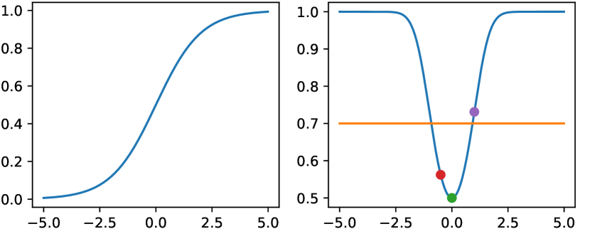
Figure 1: Logistic function and non-monotonic classifier (for Example 1).

As the previous example illustrates, the positive/negative effect of a feature can only be determined locally in an environment that depends on the input. In our previous example, the closer the negative input is to $0$, the smaller is the environment in which we can expect scores that are qualitatively faithful to the model. This is because the effect switches from negative to positive at $0$. Such a behaviour may emerge in many domains. For example, when predicting health risks, the probability often increases when particular health markers deviate substantially from a default value (for instance, both underweight and overweight and both low and high blood pressure could be seen as red flags). Furthermore, multiple changes in the behaviour of a classifier can naturally occur for geographic features, e.g. latitude and longitude in real estate datasets: here, when predicting property demand, assuming monotonic behaviour is unrealistic because the popularity of neighbouring areas may be unrelated.

4.3 Faithfulness and Gradients

We will now argue that faithfulness is closely related to gradients when we try to explain differentiable classifiers over continuous data. Let us first note that the local behaviour of a function can be precisely captured by its partial derivatives. Since many probabilistic classifiers like logistic regression and many neural networks correspond to differentiable functions, it seems worthwhile to work towards a characterization of faithfulness in terms of differentiability. Following [14], we call a function $f:D\rightarrow\mathbb{R}$ with domain $D\subseteq\mathbb{R}^{n}$ differentiable at $\mathbf{x}\in D$ iff there is a vector $g\in\mathbb{R}^{n}$ such that $\lim_{\mathbf{y}\rightarrow 0}\frac{f(\mathbf{x}+\mathbf{y})-f(\mathbf{x})-g^{\top}\mathbf{y}}{\|\mathbf{y}\|}=0$. Intuitively, this means that $f(\mathbf{x}+\mathbf{y})\approx f(\mathbf{x})+g^{\top}\mathbf{y}$, that is, $f$ can be approximated locally by a linear function. The vector $g$ is called the gradient of $f$ at $\mathbf{x}$ and denoted by $\nabla f(\mathbf{x})$. Its i-th component $g_{i}$ is denoted by $\frac{\partial f}{\partial x_{i}}(\mathbf{x})$ and is called the $i$-th partial derivative of $f$ at $\mathbf{x}$. Intuitively, $\frac{\partial f}{\partial x_{i}}(\mathbf{x})$ measures the growth of $f$ at $\mathbf{x}$ along the i-th dimension. In the following proofs, we will often use the fact that the partial derivative of a function $f$ can be written as $\frac{\partial f}{\partial x_{i}}(\mathbf{x})=\lim_{h\rightarrow 0}\frac{f(\mathbf{x}+he_{i})-f(\mathbf{x})}{h}$, where $e_{i}$ denotes the i-th unit vector [14].

We first note that the partial derivatives of features give us a locally qualitative faithful attribution method for every differentiable probabilistic classifier. We call the corresponding attribution method Gradient-scoring.

Definition 3 (Gradient-scoring).

The attribution method $g_{\operatorname{C},l}$ defined by $g_{\operatorname{C},l}(\mathbf{x})=\nabla\operatorname{C}_{l}(\mathbf{x})$ is called Gradient-scoring.

Proposition 1.

If $\operatorname{C}$ is differentiable, then Gradient-scoring is locally qualitatively faithful to $\operatorname{C}$.

Proof.

We have to check that the two cases in the definition of a local qualitative faithful attribution method are satisfied for $g_{\operatorname{C},l}$. Assume first that the score of the i-th feature for label $l$ is positive, that is, $0<g_{\operatorname{C},l}(\mathbf{x})_{i}=\frac{\partial\operatorname{C}_{l}}{\partial x_{i}}(\mathbf{x})=\lim_{h\rightarrow 0}\frac{\operatorname{C}_{l}((\mathbf{x}_{-i},x_{i}+h))-\operatorname{C}_{l}(\mathbf{x})}{h}$. For the case $x>x_{i}$, let $h=x-x_{i}>0$. Then we have $\operatorname{C}_{l}(\mathbf{x}_{-i},x)-\operatorname{C}_{l}(\mathbf{x})=\operatorname{C}_{l}(\mathbf{x}_{-i},x_{i}+h)-\operatorname{C}_{l}(\mathbf{x})=h\cdot\frac{\operatorname{C}_{l}(\mathbf{x}_{-i},x_{i}+h)-\operatorname{C}_{l}(\mathbf{x})}{h}\approx h\cdot\frac{\partial\operatorname{C}_{l}}{\partial x_{i}}(\mathbf{x})>0$ if $x$ is sufficiently close to $x_{i}$. Hence, there exists an $\epsilon>0$ such that $\operatorname{C}_{l}(\mathbf{x})<\operatorname{C}_{l}(\mathbf{x}_{-i},x)$ if $|x-x_{i}|<\epsilon$ as desired. The case $x<x_{i}$ can be checked symmetrically. The second case for $g_{\operatorname{C},l}(\mathbf{x})_{i}<0$ follows analogously. ∎

We illustrate the desirable behaviour of Gradient-scoring in two simple examples.

Example 2.

Consider again the non-linear classifier $\operatorname{C}_{1}(x)=\phi_{l}(x^{2})$ from Example 1. As we noted there, there can be no strongly faithful attribution method for $\operatorname{C}_{1}$, so a locally faithful explanation is the best that we can hope for. It is well known that the derivative of the logistic function is $\phi_{l}^{\prime}(x)=\frac{\exp(x)}{(1+\exp(x))^{2}}$. Note, in particular, that $\phi_{l}^{\prime}(x)>0$ for all $x\in\mathbb{R}$ because both the numerator and denominator are necessarily positive. The derivative of our classifier is $\operatorname{C}_{1}^{\prime}(x)=2x\cdot\phi_{l}^{\prime}(x^{2})$, which is negative for $x<0$ and positive for $x>0$. By looking at Figure 1, we can see that the derivative is indeed locally qualitatively faithful to the classifier, as it is mononotonically decreasing for $x<0$ and monotonically increasing for $x>0$. This is not a coincidence, of course, because the derivative captures exactly the local change of a function.

Example 3.

As another example, let us consider a linear classifier. A logistic regression classifier for a binary classification problem has the form $\operatorname{C}(\mathbf{x})=\phi_{l}(\sum_{i=1}^{n}w_{i}\cdot\mathbf{x}_{i})$, where $w_{i}\in\mathbb{R}$. The partial derivative wrt. the i-th feature is $\frac{\partial\operatorname{C}}{\partial x_{i}}(\mathbf{x})=w_{i}\cdot\phi_{l}^{\prime}(\sum_{i=1}^{n}w_{i}\cdot\mathbf{x}_{i})$. As before, the sign depends only on $w_{i}$. So the score is positive if $w_{i}>0$, negative if $w_{i}<0$ and 0 if $w_{i}=0$. It is clear from the definition of logistic regression that the weights reflect the true behaviour of the classifier, so Gradient-scoring is indeed a qualitative faithful attribution method. In fact, it is even globally strongly qualitatively faithful. Of course, the qualitative influence on the model can be directly seen by looking at the coefficients, but logistic regression is a reasonable test for the reliability of an attribution method. We will use this in Section 6 to evaluate the faithfulness of various attribution methods.

Let us note that every linear classifier is monotonic. If the coefficient of the $i$-th feature is positive (negative), the classifier is monotonically increasing (decreasing) wrt. the i-th feature. Let us note that Gradient-scoring is globally qualitative faithful for every monotonic classifier.

Proposition 2.

If $\operatorname{C}$ is differentiable and monotonic, then Gradient-scoring is globally qualitatively faithful to $\operatorname{C}$.

Proof.

We prove the claim by going through the two cases again. If $g_{\operatorname{C},l}(\mathbf{x})_{i}>0$, then the partial derivative is positive at this point. Hence, $g_{\operatorname{C},l}(.)_{i}$ is strictly increasing at this point. Since $g_{\operatorname{C},l}$ is monotonic, $g_{\operatorname{C},l}(.)_{i}$ must be increasing (not necessarily strictly increasing) on the whole domain of the $i$-th feature. If $x>x_{i}$, there must be a $y\in(x_{i},x)$ such that $\operatorname{C}_{l}(\mathbf{x})<\operatorname{C}_{l}(\mathbf{x}_{-i},y)\leq\operatorname{C}_{l}(\mathbf{x}_{-i},x)$ where the strict inequality follows from strict monotonicity at $\mathbf{x}$ and the second inequality from monotonicity on the whole domain. Symmetrically, one can check that $\operatorname{C}_{l}(\mathbf{x})>\operatorname{C}_{l}(\mathbf{x}_{-i},x)$ for all $x<x_{i}$.

The second case from the definition of qualitative faithfulness can be checked symmetrically. ∎

Let us note that the result is actually slightly stronger: If the classifier is monotonic wrt. a particular feature, then Gradient-scoring is globally qualitatively faithful. If it is strictly monotonic, then Gradient-scoring is globally strongly qualitatively faithful.

In summary, Gradient-scoring is locally qualitatively faithful for every differentiable classifier; it is globally qualitatively faithful for monotonic differentiable classifiers. Thus, given that there can be no attribution method that is globally qualitatively faithful for non-monotonic classifiers (as illustrated in Example 1) Gradient-scoring gives us the strongest guarantees that we can hope for.

There can be other locally qualitatively faithful attribution methods for differentiable probabilistic classifiers, of course. However, as we explain next, they all must be closely related to Gradient-scoring. Intuitively, the following proposition states that an attribution method for a differentiable classifier can only be locally qualitatively faithful if the sign of its score equals the sign of the partial derivative. In other words, every qualitatively faithful attribution method must be qualitatively equivalent to Gradient-scoring.

Proposition 3.

If $\operatorname{C}$ is differentiable and there exists an attribution method $s_{\operatorname{C},l}:{1,\dots,k}\rightarrow\mathbb{R}$ that is locally qualitatively faithful to $\operatorname{C}$, then for all $i=1,\dots,k$, for all inputs $\mathbf{x}\in\mathcal{D}$ and all labels $l\in L$, we have

1. if $s_{\operatorname{C},l}(\mathbf{x})_{i}>0$, then $g_{\operatorname{C},l}(\mathbf{x})_{i}\geq 0$, and

2. if $s_{\operatorname{C},l}(\mathbf{x})_{i}<0$, then $g_{\operatorname{C},l}(\mathbf{x})_{i}\leq 0$.

Proof.

Consider the case $s_{\operatorname{C},l}(\mathbf{x})_{i}>0$. Since $s_{\operatorname{C},l}$ is locally qualitatively faithful, we have that, for all $h$ that are sufficiently close to $0$, $\operatorname{C}_{l}(\mathbf{x}_{-i},x_{i}+h)-\operatorname{C}_{l}(\mathbf{x})>0$ if $h>0$ and $\operatorname{C}_{l}(\mathbf{x}_{-i},x_{i}+h)-\operatorname{C}_{l}(\mathbf{x})<0$ if $h<0$. Therefore, $\frac{\operatorname{C}_{l}(\mathbf{x}_{-i},x_{i}+h)-\operatorname{C}_{l}(\mathbf{x})}{h}>0$ and $\frac{\partial\operatorname{C}_{l}}{\partial x_{i}}(\mathbf{x})=\lim_{h\rightarrow 0}\frac{\operatorname{C}_{l}(\mathbf{x}_{-i},x_{i}+h)-\operatorname{C}_{l}(\mathbf{x})}{h}\geq 0$.

The second item follows symmetrically. ∎

4.4 Summary

We quickly summarize the main points of this section. An attribution method should be qualitatively faithful. However, as demonstrated in Example 1, we cannot guarantee global or strong faithfulness without making additional assumptions about the nature of the classifier that we want to explain. For non-monotonic classifiers, attributive explanations typically cannot exhibit strong qualitative faithfulness. We showed that Gradient-scoring is always locally qualitatively faithful (Proposition 1) and that every locally qualitatively faithful attribution method must be qualitatively equivalent to Gradient-scoring (Proposition 3). Stronger guarantees can only be given for monotonic classifiers and Gradient-scoring guarantees global qualitative faithfulness for these classifiers (Proposition 2). As we will demonstrate in Section 6, this is not the case for some other popular attribution methods. Let us also note that monotonicity alone is not sufficient to allow for strongly faithful explanations. For example, a monotonically increasing function may be constant for a while before it continues increasing. To guarantee strongly qualitatively faithful explanations, we have to assume that a classifier is, for every feature, either strictly monotonic or constant. In this case, every locally qualitative faithful attribution method is also strongly qualitatively faithful.

5 Quantitative Faithfulness

In the previous section, we showed that every qualitatively faithful attribution method must be qualitatively equivalent to Gradient-scoring. However, usually, we want that the attribution method is also quantitatively faithful in the sense that a larger score reflects a larger influence of a feature on the prediction. This quantitative faithfulness could be formalized in different ways. One intuitive way is to demand that the change in output of the prediction model when increasing a feature is proportional to its score. Formally,

$$\operatorname{C}_{l}(\mathbf{x}_{-i},x_{i}+h)\approx\operatorname{C}_{l}(\mathbf{x})+h\cdot s_{\operatorname{C},l}(\mathbf{x})_{i}.$$ (1)

More generally, we can demand

$$\operatorname{C}_{l}(\mathbf{x}+\mathbf{h})\approx\operatorname{C}_{l}(\mathbf{x})+\mathbf{h}^{\top}s_{\operatorname{C},l}(\mathbf{x})=\operatorname{C}_{l}(\mathbf{x})+\sum_{i=1}^{k}h_{i}\cdot s_{\operatorname{C},l}(\mathbf{x})_{i},$$ (2)

where equation (1) is recovered when we let $\mathbf{h}$ be the $i$-th unit vector. Let us note that both conditions are trivially satisfied for small $h$ in our setting. This is because our classifier is differentiable and therefore continuous by assumption. Hence, whenver $\mathbf{h}\approx 0$, we also have $\operatorname{C}_{l}(\mathbf{x}+\mathbf{h})\approx\operatorname{C}_{l}(\mathbf{x})$ (by continuity) and $\mathbf{h}^{\top}s_{\operatorname{C},l}(\mathbf{x})\approx 0$ (because $s_{\operatorname{C},l}(\mathbf{x})$ is constant). To make the condition non-trivial, we have to demand that the approximation error goes faster to $0$ than $\mathbf{h}$. We let $e(\mathbf{h})=\operatorname{C}_{l}(\mathbf{x}+\mathbf{h})-\operatorname{C}_{l}(\mathbf{x})-\mathbf{h}^{\top}s_{\operatorname{C},l}(\mathbf{x})$ denote the error of the approximation when changing the input by $\mathbf{h}$. Then we can rewrite (2) more precisely as

$$\operatorname{C}_{l}(\mathbf{x}+\mathbf{h})=\operatorname{C}_{l}(\mathbf{x})+\mathbf{h}^{\top}s_{\operatorname{C},l}(\mathbf{x})+e(\mathbf{h}).$$ (3)

To get a non-trivial condition, we require that $e(\mathbf{h})$ goes significantly faster to $0$ than $\mathbf{h}$, that is, we additionally demand that $\lim_{\mathbf{h}\rightarrow 0}\frac{e(h)}{\|\mathbf{h}\|}=0$.

Definition 4 (Local Quantitative Faithfulness).

An attribution method $s_{\operatorname{C},l}:{1,\dots,k}\rightarrow\mathbb{R}$ is called locally quantitatively faithful to $\operatorname{C}$ if for all inputs $\mathbf{x}\in\mathcal{D}$, for all labels $l\in L$, for all $i=1,\dots,k$ and for all $\mathbf{h}$ such that $\mathbf{x}+\mathbf{h}\in\mathcal{D}$, we have $\operatorname{C}_{l}(\mathbf{x}+\mathbf{h})=\operatorname{C}_{l}(\mathbf{x})+\mathbf{h}^{\top}s_{\operatorname{C},l}(\mathbf{x})+e(\mathbf{h}),$ where $e(\mathbf{h})$ is an error term with $\lim_{\mathbf{h}\rightarrow 0}\frac{e(h)}{\|\mathbf{h}\|}=0$.

Gradient-scores satisfy local quantitative faithfulness by definition. More interestingly, the property characterizes Gradient-scoring in the sense that it is the only attribution method that does so.

Proposition 4.

If $\operatorname{C}$ is differentiable, then $s_{\operatorname{C},l}$ is locally quantitative faithful to $\operatorname{C}$ if and only if $s_{\operatorname{C},l}=g_{\operatorname{C},l}$.

Proof.

To see that $g_{\operatorname{C},l}$ satisfies local quantitative faithfulness, note that $\lim_{\mathbf{h}\rightarrow 0}\frac{e(h)}{\|\mathbf{h}\|}=\lim_{\mathbf{h}\rightarrow 0}\frac{\operatorname{C}_{l}(\mathbf{x}+\mathbf{h})-\operatorname{C}_{l}(\mathbf{x})-\mathbf{h}^{\top}g_{\operatorname{C},l}(\mathbf{x})}{\|\mathbf{h}\|}=0$ because $\operatorname{C}_{l}$ is differentiable (see Section 4.3 to recall the definition of differentiability).

To show that Gradient-scoring is the only attribution method that satisfies this property, consider an arbitrary attribution method $s_{\operatorname{C},l}$ that satisfies local quantitative faithfulness. We show that it is equal to Gradient-scoring by showing that for all inputs $\mathbf{x}$ and for all feature dimensions $i$, we have $|g_{\operatorname{C},l}(\mathbf{x})_{i}-s_{\operatorname{C},l}(\mathbf{x})_{i}|<\epsilon$ for every $\epsilon>0$. Since $\epsilon$ can be arbitrarily small, we must have $g_{\operatorname{C},l}(\mathbf{x})_{i}=s_{\operatorname{C},l}(\mathbf{x})_{i}$, which proves the claim. Let $e_{g}$ and $e_{s}$ denote the error functions for $g_{\operatorname{C},l}$ and $s_{\operatorname{C},l}$, respectively. Then we can find an $h>0$ such that for all unit vectors $u_{i}$, we have $\big{|}\frac{e_{g}(h\cdot u_{i})}{h}\big{|}<\frac{\epsilon}{2}$ and $\big{|}\frac{e_{s}(h\cdot u_{i})}{h}\big{|}<\frac{\epsilon}{2}$. Then

$$|g_{\operatorname{C},l}(\mathbf{x})_{i}-s_{\operatorname{C},l}(\mathbf{x})_{i}| =\big{|}\frac{h\cdot g_{\operatorname{C},l}(\mathbf{x})_{i}-h\cdot s_{\operatorname{C},l}(\mathbf{x})_{i}}{h}\big{|}$$

$$=\big{|}\frac{h\cdot g_{\operatorname{C},l}(\mathbf{x})_{i}-\operatorname{C}_{l}(\mathbf{x}+h\cdot u_{i})+\operatorname{C}_{l}(\mathbf{x})}{h}$$

$$\quad+\frac{\operatorname{C}_{l}(\mathbf{x}+h\cdot u_{i})-\operatorname{C}_{l}(\mathbf{x})-s_{\operatorname{C},l}(\mathbf{x})_{i})\cdot h}{h}\big{|}$$

$$\leq\big{|}\frac{e_{g}(h\cdot u_{i})}{h}\big{|}+\big{|}\frac{e_{s}(h\cdot u_{i})}{h}\big{|}<\epsilon,$$

which completes the proof. ∎

Intuitively, if any other attribution method can guarantee that the scores are proportional to the actual influence of the features (it satisfies equation (2)), then the method is either equivalent to gradient scoring or it is based on an inferior approximation of the model, that is, it does not satisfy $\lim_{h\rightarrow 0}\frac{e(h)}{\|\mathbf{h}\|}=0$. In more precise terms, we can state that the approximation error with respect to $g_{\operatorname{C},l}$ goes significantly faster to $0$ than the error with respect to every other attribution method.

Proposition 5.

If $\operatorname{C}$ is differentiable, then for every attribution method $s_{\operatorname{C},l}\neq g_{\operatorname{C},l}$, we have $\lim_{\mathbf{h}\rightarrow 0}\frac{e_{g}(h)}{e_{s}(h)}=0$, where $e_{g}$ and $e_{s}$ denote the error functions for $g_{\operatorname{C},l}$ and $s_{\operatorname{C},l}$, respectively.

Proof.

Since $s_{\operatorname{C},l}\neq g_{\operatorname{C},l}$, Proposition 4 implies $\lim_{\mathbf{h}\rightarrow 0}\frac{e_{s}(h)}{\|\mathbf{h}\|}\neq 0$. Hence, we can find an $\epsilon>0$ such that $\lim_{\mathbf{h}\rightarrow 0}\big{|}\frac{e_{s}(h)}{\|\mathbf{h}\|}\big{|}\geq\epsilon>0$. Then we have $\lim_{\mathbf{h}\rightarrow 0}\frac{e_{g}(h)}{e_{s}(h)}=\lim_{\mathbf{h}\rightarrow 0}\frac{\frac{e_{g}(h)}{\|h\|}}{\frac{e_{s}(h)}{\|h\|}}\leq\frac{0}{\epsilon}=0.$ ∎

Similar to qualitative faithfulness, we usually cannot expect to find a "globally" quantitatively faithful attribution method. Let us note that while monotonicity of a classifier allows global qualitative faithfulness, it is not sufficient to allow "global" quantitative faithfulness. This is because a monotonic function can still increase (or decrease) faster and slower in different regions of its domain. Conceptually, stronger guarantees can be obtained by moving from just the gradient (a first-order Taylor approximation) to higher-order Taylor approximations of the classifier. For example, scores for the influence of pairs of features can be obtained from the Hessian matrix. However, this would also increase the computational cost considerably and the explanation would be less succinct (but more accurate).

6 Experiments

In this section, we investigate to which extent different attribution methods (see Section 6.2) are faithful to a classifier and how close they are to each other on three continuous datasets (see Section 6.1). To evaluate faithfulness, we consider Logistic Regression classifiers, where the sign of coefficients represent the true qualitative effect of features on models and their magnitude their impact (see Section 6.4). To also compare attribution methods for non-linear models, we consider Multilayer Perceptrons with unknown ground truth (see Section 6.5). The code for all experiments is available at

https://github.com/XiangYin2021/Revisit-Faithfulness

6.1 Datasets

We use three binary classification problems with continuous features from the UCI machine learning repository.

BNAT: The Banknote Authentication data set consists of image information features (like entropy of image, or variance of Wavelet Transformed image) of genuine and forged banknotes. The label identifies whether a banknote is genuine.

WDBC: The Breast Cancer Wisconsin (Diagnostic) data set [19] contains features of cell nuclei of breast mass images, and their corresponding diagnosis (Benign or Malignant) as labels.

PIMA: The PIMA Indians Diabetes data set [3] contains physical indicator features of females and their diagnosis of diabetes as label.

Table 1 summarizes some basic statistics of the data sets.

Table 1: Basic data set statistics.

Dataset	Instances	Features	Label
BKNT	1372	5	Binary
WDBC	569	30	Binary
PIMA	768	8	Binary

6.2 Attribution Methods

We compare Gradient-scoring to three popular attribution methods.

LIME [16] is a model-agnostic local explanation method. In order to explain the output at one data point, LIME first perturbs this point to generate several points in a small neighborhood, and weighs the perturbed points based on their distance to the original point. LIME then trains a linear model to explain the original point by the weights of the linear model. We used the LIME implementation from https://github.com/marcotcr/lime and applied the LIMETabularExplainer.

SHAP [13] uses the Shapley value from coalitional game theory to compute the contribution of each feature to the prediction. As the Shapley value is a discrete concept, SHAP relies heavily on sampling when being applied to continuous features. We used the SHAP implementation from https://github.com/slundberg/shap and show results for the KernelExplainer. As SHAP did not perform well in the experiments, we tried different settings, but they did not improve the outcome.

SILO [6] is a non-parametric regression method, but can also be seen as an attribution method. It first uses random forests to compute weights of data points in the training set, and then selects supervised neighbourhoods to construct local linear models. The coefficients of the linear model can again be used to assign scores to features. We also mentioned MAPLE [15] before, which extends SILO by a feature selection method. However, as we want to find out to which extent different methods capture the true effects of all features, we will consider only SILO in our experiments. We use the MAPLE implementation from https://github.com/GDPlumb/MAPLE and omit the feature selection step. We configured it with n_estimators=200; min_sample_leaf=10 and linear_model=Ridge.

6.3 Setup

6.3.1 Hardware

We ran all experiments on a MacBook Pro (OS: macOS Monterey 12.0.1; Processor: 2.3GHz, dual-core Intel Core i5; Memory: 8GB).

6.3.2 Classifiers

We used the default training settings of scikit-learn for Logistic Regression (LR) and Multilayer Perceptrons (MLP) with the following modifications:

• LR: max_iter=500.

• MLP: We experimented with different numbers of hidden layers and neurons per layer and eventually used five hidden layers with eight neurons in each layer. The maximum number of iterations (max_iter) was set to 1000.

Table 2 shows the performance of the classifiers on our datasets.

Table 2: Accuracy and F1-score for Classifiers

Classifier	Dataset	Accuracy	F1-score
	PIMA	0.760	0.565
LR	BKNT	0.964	0.958
	WDBC	0.956	0.937
	PIMA	0.721	0.566
MLP	BKNT	0.978	0.975
	WDBC	0.982	0.976

6.4 Experiments with Logistic Regression (LR)

In our first set of experiments, we compute explanations for LR because its feature weights can be seen as representing the true effect of features on the LR classifier. One has to consider that the logistic function is applied to the linear combination of features, so the feature weights do not represent the true quantitative effect. However, as the logistic function is monotonic, the weights show the true qualitative effect and the true order of the impact of features.

We used the LR implementation of scikit-learn in our experiments. Gradient-scores can be easily computed analytically from the weights as explained in Example 3.

To evaluate how well different explanation methods reflect the true effect of features on the classifier, we computed Spearman’s rank correlation between the LR weights and the attribution scores in Table 3. We averaged the correlation over all inputs from the test set for each dataset. Spearman’s rank correlation measures the strength of the monotonic relationship between two variables. As opposed to Pearson’s correlation, it can also capture non-linear relationships and seems therefore well suited for the task. The gradient shows perfect correlation with the weights. This can also be seen analytically because the gradient corresponds to the feature weight multiplied by a constant that depends on the point (see Example 3). LIME is reasonably close for all datasets. SILO does well on two datasets, but does not work well on WDBC. SHAP does not show any significant correlation with the weights on any dataset.

Table 3: Average Spearman rank correlation between LR weights and different explanation methods on test data.

Dataset	GRAD	SILO	LIME	SHAP
PIMA	1.000	0.989	0.976	0.166
BKNT	1.000	0.975	1.000	-0.073
WDBC	1.000	0.378	0.986	0.272

To give a better picture of the output of different attribution methods, Tables 4 - 6, show the LR weights and the scores that have been assigned to features by the different attribution methods for the first test data point of our three datasets, respectively. We ordered the features by their logistic regression weights, so that the qualitative score and their order can be compared easily.

Table 4: LR weights and feature scores for the first test data point of the BNKT Dataset.

	Weight	Grad	SILO	LIME	SHAP
vwti	-10.240	-0.536	-0.748	-0.270	-0.443
swti	-7.508	-0.393	-0.571	-0.212	-0.014
cwti	-7.001	-0.366	-0.530	-0.167	-0.042
entr	0.284	0.015	0.021	0.006	0.003

Table 5: LR weights and feature scores for the first test data point of the PIMA Dataset.

	Weight	Grad	SILO	LIME	SHAP
bloo	-0.734	-0.139	-0.146	-0.022	-0.011
insu	0.021	0.004	-0.004	0.000	-0.000
skin	0.581	0.110	0.118	0.018	-0.002
age	1.078	0.205	0.232	0.041	0.025
diab	1.254	0.238	0.275	0.033	0.003
preg	1.350	0.256	0.278	0.051	0.046
bmi	2.855	0.542	0.611	0.063	-0.006
gluc	4.920	0.934	1.068	0.153	0.041

Table 6: Five lowest and highest LR weights and corresponding feature scores for the first test data point of the WDBC Dataset.

	Weight	GRAD	SILO	LIME	SHAP
mean fractal dimension	-0.821	-0.168	-0.046	-0.021	0.016
se fractal dimension	-0.602	-0.123	-0.079	-0.015	0.022
se compactness	-0.415	-0.085	0.115	-0.011	0.009
se symmetry	-0.330	-0.068	-0.008	-0.007	0.006
se concavity	-0.143	-0.029	-0.062	-0.001	0.001
se smoothness	-0.015	-0.003	-0.058	-0.002	-0.000
se texture	-0.003	-0.001	0.225	0.001	-0.000
worst fractal dimension	0.347	0.071	0.119	0.007	-0.001
mean symmetry	0.363	0.074	0.029	0.009	-0.007
mean smoothness	0.384	0.079	-0.001	0.010	-0.002
se concave points	0.408	0.083	-0.028	0.011	-0.008
mean compactness	0.571	0.117	-0.311	0.016	-0.016
se area	0.677	0.139	-0.078	0.011	-0.002
se perimeter	0.737	0.151	-0.407	0.013	-0.009
worst compactness	0.799	0.163	0.176	0.023	-0.009
se radius	0.956	0.196	0.515	0.018	-0.006
worst symmetry	1.172	0.240	0.052	0.024	0.004
worst concavity	1.387	0.284	0.027	0.042	-0.004
mean concavity	1.405	0.288	0.163	0.048	-0.024
mean area	1.446	0.296	-0.953	0.042	0.003
mean texture	1.452	0.297	0.262	0.038	0.038
worst smoothness	1.472	0.301	0.266	0.041	0.005
worst area	1.638	0.335	0.224	0.043	0.006
mean perimeter	1.704	0.349	0.661	0.053	-0.005
mean radius	1.721	0.352	0.621	0.053	-0.002
mean concave points	1.851	0.379	0.079	0.064	-0.009
worst texture	2.069	0.423	-0.212	0.063	0.060
worst perimeter	2.077	0.425	0.884	0.064	-0.004
worst radius	2.260	0.462	-0.583	0.073	0.004
worst concave points	2.679	0.548	0.177	0.111	0.021

Across all datasets, we can see that Gradient-scores always correctly capture the qualitative effect and the order of features as the theory suggests. Since SILO and LIME are based on linear approximations of the model, we should expect a similar picture. However, as they depend on sampling, the result may be more noisy. The experiments show indeed that both capture the true effect of features relatively well. However, sometimes, the order is not captured completely correctly and there can be problems with the sign. For example, SILO assigns a negative score to WORST TEXTURE and WORST RADIUS in Table 6 even though they have a large positive weight. LIME works generally better, but does not capture the true order perfectly. This can be seen, for example, for AGE, DIAB and PREG in Table 5. However, while SILO and LIME have problems distinguishing features that are close, they perform reasonably well overall. The results for SHAP, in contrast, look quite random overall and often do not seem to reflect the true effect of features on the classifier.

6.5 Experiments with Multilayer Perceptrons (MLPs)

LR is well suited for experiments because the true effect of features can be seen from the weights. However, in general, we are also interested in explaining non-linear classifiers. Unfortunately, in this case, an objective ground truth is rarely available. There has been some work recently on creating synthetic prediction models with known ground truth [9], but the work does not cover non-linear classifiers for continuous data (they only consider synthetic linear regression models for tabular data) and rely on the assumption that the models correctly learnt relationships from artificially generated data. We feel that the gradient does represent the ground truth because it exactly captures the local growth of a function. This intuitive idea is made precise in Definition 4 and Proposition 4. Let us note that the gradient is also used as the ground truth for the synthetic linear regression models in [9]. However, it is, of course, a philosophical question whether this is what the scores should represent. In lack of an objective ground truth, we simply compare the Gradient-scores to the scores under other attribution methods. While a low correlation is difficult to interpret, a high correlation basically indicates that the methods give similar explanations to Gradient-scoring.

We used the MLP implementation from scikit-learn for the experiments in this section. For many libraries, gradients can be computed using their auto-differentiation functionality. However, we simply approximated the gradient by the symmetric difference quotient $\tilde{g}(x)=\frac{f(x+\varepsilon)-f(x-\varepsilon)}{2\varepsilon}$ in our experiments. Table 7 shows the Spearman rank correlation between the Gradient-score and the other methods. The correlation with LIME is high. This can be expected analytically because LIME just computes another linear approximation of the model. The correlation with SILO is lower, in particular, for WDBC. SHAP again does not show any correlation with the Gradient-score. As no objective ground truth is available, we cannot objectively say that one method gives better explanations than another. However, we feel that Gradient-scores are favorable because they have a clearly defined meaning (they capture the local sensitivity of the model with respect to the feature) and are not susceptible to noise caused by sampling. In particular, it does not seem clear what SHAP scores actually mean in a setting where features are continuous because the theory of Shapley values has been developed in a discrete setting and SHAP scores rely heavily on approximation and sampling when features are continuous.

Table 7: Average Spearman rank correlation between Gradient-scoring and other explanation methods on test data with MLPs.

Dataset	GRAD	SILO	LIME	SHAP
PIMA	1.000	0.868	0.905	0.256
BKNT	1.000	0.640	0.837	0.260
WDBC	1.000	0.293	0.938	0.297

6.6 Runtime Performance

Overall, we feel that linear attribution methods like Gradient-scoring, LIME and SILO are more natural in the continuous setting because they have a clear interpretation. LIME is highly correlated with Gradient-scoring, so a natural question arises as to why one should prefer one method over the other. One consideration to take into account is runtime performance. Gradient-scores are easy to compute in linear time with respect to the number of features. Ideally, this should be done using the auto-differentiation functionalities of libraries. When approximating the gradient using the symmetric difference quotient, one has to consider the usual numerical approximation problems that can occur when the classifier has large partial derivatives (e.g., when the neural network has very large weights). The runtime of linear explainers like LIME and SILO is also linear, but additionally depends on the number of samples that are taken and on the training procedure for learning the local substitute model. In particular, while a smaller sample size may result in faster runtime, the scores may be too noisy if the sample size is chosen too small. SHAP is usually most difficult to compute and relies heavily on sampling. The complexity of computing SHAP scores has been analyzed recently and is intractable in many interesting cases [23]. As our datasets are rather small, all methods work in reasonable time. For completeness, we show runtime results in milliseconds in Table 8. As one may expect, computing Gradient-scores is significantly faster than computing SILO and LIME scores, which, in turn, is significantly faster than computing SHAP scores.

Table 8: Runtime for different explanation methods (in ms).

	DATA	GRAD	SILO	LIME	SHAP
	PIMA	0.01	14.54	8.68	594.19
LR	BKNT	0.01	13.30	30.99	182.63
	WDBC	0.02	14.10	18.74	3033.67
	PIMA	0.24	13.10	9.60	603.36
MLPs	BKNT	0.32	13.31	33.33	178.32
	WDBC	0.28	14.28	18.46	3167.71

7 Conclusions

We revisited faithfulness of attribution methods in the setting where the prediction model is differentiable and features are continuous. While sampling and an empirical notion of faithfulness (based on the empirical accuracy of a local substitute model) seem difficult to avoid in the discrete setting, the continuous setting allows for more analytical tools. We therefore proposed two analytical notions of faithfulness (qualitative and quantitative) and showed that they are satisfied by Gradient-scoring and, to some extent, only by Gradient-scoring. In particular, quantitative faithfulness completely characterizes Gradient-scoring in the sense that every explanation method that satisfies this property must be equivalent to Gradient-scoring (Proposition 4). Roughly speaking, every attribution method that guarantees that the scores are proportional to the changes in the output of the classifier is either equivalent to gradient-scoring or is based on an inferior approximation of the classifier.

To back up the theory, we investigated empirically to which extent different attribution methods explain the true behaviour of logistic regression. Linear attribution methods like LIME and SILO do reasonably well, but perform worse than Gradient-scoring. SHAP does not seem to capture the true behaviour of the classifier at all. For non-linear classifiers, there is still some correlation between linear attribution methods and the gradient. While it is hard to tell objectively which explanations are better in this case, Gradient-scores seem preferable. Not only do they have a clearly defined analytical meaning and are not susceptible to noise caused by sampling, but they can also be computed easily.

Overall, we believe that Gradient-scoring is the most suitable method for the continuous setting that we considered here. In particular, SHAP does not seem well suited for this setting as the SHAP scores for logistic regression seem completely uncorrelated with the actual weights. In general, it seems that more research is necessary on clarifying what feature scores under different methods actually represent. In particular, they can potentially be made more accurate by adding scores to selected pairs (collections) of features similar to how second-order (higher-order) terms approve the accuracy of Taylor approximations. However, naturally, there is a trade-off between accuracy of the explanation, computational cost and comprehensibility.

References

- [1] Adadi, A., and Berrada, M. Peeking inside the black-box: a survey on explainable artificial intelligence (xai). IEEE access 6 (2018), 52138–52160.
- [2] Agarwal, S., Jabbari, S., Agarwal, C., Upadhyay, S., Wu, S., and Lakkaraju, H. Towards the unification and robustness of perturbation and gradient based explanations. In International Conference on Machine Learning ICML (2021), M. Meila and T. Zhang, Eds., vol. 139 of Proceedings of Machine Learning Research, PMLR, pp. 110–119.
- [3] Alcalá-Fdez, J., Fernández, A., Luengo, J., Derrac, J., García, S., Sánchez, L., and Herrera, F. Keel data-mining software tool: data set repository, integration of algorithms and experimental analysis framework. Journal of Multiple-Valued Logic & Soft Computing 17 (2011).
- [4] Ancona, M., Ceolini, E., Öztireli, C., and Gross, M. Towards better understanding of gradient-based attribution methods for deep neural networks. In International Conference on Learning Representations (2018).
- [5] Baehrens, D., Schroeter, T., Harmeling, S., Kawanabe, M., Hansen, K., and Müller, K.-R. How to explain individual classification decisions. The Journal of Machine Learning Research 11 (2010), 1803–1831.
- [6] Bloniarz, A., Talwalkar, A., Yu, B., and Wu, C. Supervised neighborhoods for distributed nonparametric regression. In Artificial Intelligence and Statistics (2016), PMLR, pp. 1450–1459.
- [7] Garreau, D., and Luxburg, U. Explaining the explainer: A first theoretical analysis of lime. In International Conference on Artificial Intelligence and Statistics (2020), PMLR, pp. 1287–1296.
- [8] Ghorbani, A., Abid, A., and Zou, J. Interpretation of neural networks is fragile. In Proceedings of the AAAI Conference on Artificial Intelligence (2019), vol. 33, pp. 3681–3688.
- [9] Guidotti, R. Evaluating local explanation methods on ground truth. Artificial Intelligence 291 (2021), 103428.
- [10] Heo, J., Joo, S., and Moon, T. Fooling neural network interpretations via adversarial model manipulation. Advances in Neural Information Processing Systems 32 (2019), 2925–2936.
- [11] Lipton, Z. C. The mythos of model interpretability: In machine learning, the concept of interpretability is both important and slippery. Queue 16, 3 (2018), 31–57.
- [12] Lundberg, S. M., and Lee, S.-I. A unified approach to interpreting model predictions. In Proceedings of the 31st international conference on neural information processing systems (2017), pp. 4768–4777.
- [13] Lundberg, S. M., Nair, B., Vavilala, M. S., Horibe, M., Eisses, M. J., Adams, T., Liston, D. E., Low, D. K.-W., Newman, S.-F., Kim, J., et al. Explainable machine-learning predictions for the prevention of hypoxaemia during surgery. Nature Biomedical Engineering 2, 10 (2018), 749.
- [14] Nocedal, J., and Wright, S. Numerical optimization. Springer Science & Business Media, 2006.
- [15] Plumb, G., Molitor, D., and Talwalkar, A. Model agnostic supervised local explanations. In Proceedings of the 32nd International Conference on Neural Information Processing Systems (2018), pp. 2520–2529.
- [16] Ribeiro, M. T., Singh, S., and Guestrin, C. " why should i trust you?" explaining the predictions of any classifier. In Proceedings of the 22nd ACM SIGKDD international conference on knowledge discovery and data mining (2016), pp. 1135–1144.
- [17] Ribeiro, M. T., Singh, S., and Guestrin, C. Anchors: High-precision model-agnostic explanations. In Proceedings of the AAAI conference on artificial intelligence (2018), vol. 32.
- [18] Sanchez, I., Rocktaschel, T., Riedel, S., and Singh, S. Towards extracting faithful and descriptive representations of latent variable models. AAAI Spring Syposium on Knowledge Representation and Reasoning (KRR): Integrating Symbolic and Neural Approaches 1 (2015), 4–1.
- [19] Street, W. N., Wolberg, W. H., and Mangasarian, O. L. Nuclear feature extraction for breast tumor diagnosis. In Biomedical image processing and biomedical visualization (1993), vol. 1905, International Society for Optics and Photonics, pp. 861–870.
- [20] Sundararajan, M., and Najmi, A. The many shapley values for model explanation. In International Conference on Machine Learning, ICML (2020), vol. 119 of Proceedings of Machine Learning Research, PMLR, pp. 9269–9278.
- [21] Sundararajan, M., Taly, A., and Yan, Q. Axiomatic attribution for deep networks. In International Conference on Machine Learning (2017), PMLR, pp. 3319–3328.
- [22] Szegedy, C., Zaremba, W., Sutskever, I., Bruna, J., Erhan, D., Goodfellow, I., and Fergus, R. Intriguing properties of neural networks. In International Conference on Learning Representations (ICLR) (2014).
- [23] Van den Broeck, G., Lykov, A., Schleich, M., and Suciu, D. On the tractability of shap explanations. In AAAI Conference on Artificial Intelligence (2021), pp. 6505–6513.
- [24] Wachter, S., Mittelstadt, B., and Russell, C. Counterfactual explanations without opening the black box: Automated decisions and the gdpr. Harv. JL & Tech. 31 (2017), 841.
- [25] Wang, J., Tuyls, J., Wallace, E., and Singh, S. Gradient-based analysis of nlp models is manipulable. In Conference on Empirical Methods in Natural Language Processing (EMNLP) (2020), pp. 247–258.