Masked Image Modeling with
Denoising Contrast

Abstract

Since the development of self-supervised visual representation learning from contrastive learning to masked image modeling (MIM), there is no significant difference in essence, that is, how to design proper pretext tasks for vision dictionary look-up. MIM recently dominates this line of research with state-of-the-art performance on vision Transformers (ViTs), where the core is to enhance the patch-level visual context capturing of the network via denoising auto-encoding mechanism. Rather than tailoring image tokenizers with extra training stages as in previous works, we unleash the great potential of contrastive learning on denoising auto-encoding and introduce a pure MIM method, ConMIM, to produce simple intra-image inter-patch contrastive constraints as the sole learning objectives for masked patch prediction. We further strengthen the denoising mechanism with asymmetric designs, including image perturbations and model progress rates, to improve the network pre-training. ConMIM-pretrained models with various scales achieve competitive results on downstream image classification, semantic segmentation, object detection, and instance segmentation tasks, e.g., on ImageNet-1K classification, we achieve 83.9% top-1 accuracy with ViT-Small and 85.3% with ViT-Base without extra data for pre-training. Code will be available at https://github.com/TencentARC/ConMIM.

1 Introduction

The great success of self-supervised learning in natural language processing (NLP) tasks, e.g., BERT (Devlin et al., 2019) and GPT (Radford et al., 2018; 2019), has sparked several revolutions in visual representation learning, during which the development of vision dictionary look-up is the most critical. In the age of convolutional neural networks (CNNs) (He et al., 2016; Krizhevsky et al., 2012), prominent works (He et al., 2020; Chen et al., 2020) perform self-supervised learning with a pretext task of instance-level dictionary look-up via contrastive learning as demonstrated in Figure 1(a). With the advent of vision Transformers (ViTs) (Dosovitskiy et al., 2021), the gap between vision and NLP tasks has been further narrowed since the introduction of patch-level dictionary look-up via masked image modeling in a pioneer work BEiT (Bao et al., 2022) (see Figure 1(b)).

The introduction of masked image modeling (Bao et al., 2022), inspired by masked language modeling (Devlin et al., 2019) in NLP tasks, ushers in a new fad for self-supervised learning using vision Transformers (Dosovitskiy et al., 2021), i.e., a portion of vision tokens are randomly masked and then recovered by the Transformer network being trained. Concurrent works (Dong et al., 2021; Li et al., 2022; Wei et al., 2022) make efforts to design patch-level dictionaries, image tokenizers in other words, to build proper learning objectives (i.e., vision token ids) for masked image modeling. Though advanced results can be achieved, the off-the-shelf image tokenizers, e.g., discrete VAE (Ramesh et al., 2021) used in BEiT (Bao et al., 2022), depend on extra training stages and data knowledge, rendering an inflexible two-stage pre-training paradigm.

We would like to call for a revisit of the superiority of masked image modeling over contrastive learning on self-supervised learning with vision Transformers. Since they are essentially both designed towards vision dictionary look-up, the key difference lies in the patch-level denoising auto-encoding mechanism in masked image modeling, which encourages the network’s capability to capture fine-grained visual context and semantics. As for the auto-encoding objective, we do not have to intentionally discretize the continuous visual signals as words in NLP tasks to cast the masked prediction as a classification task. Instead, we can give full play to the wisdom of contrastive learning, which has good capability to structure the visual space with semantically meaningful representations. To this end, we introduce a new pre-training method for masked image modeling, namely, ConMIM, to get rid of extra tokenizing networks by revitalizing contrastive learning, as shown in Figure 1(c).

Our ConMIM casts masked patch prediction in self-supervised image pre-training as denoising contrastive learning. The corrupted input with a large proportion of patches masked is fed into the encoder, a plain vision Transformer in general. The encoder learns to recover the representations of the masked patches, which are predicted by feeding the full input into the encoder. The training objective is formed by an intra-image inter-patch contrastive loss. To be specific, patch representations of a full input image build a dynamic dictionary, and patches from the same positions as the masked ones of the corrupted input serve as their positive keys, respectively. The remaining ones from different positions but in a same image are the negative keys. To further improve the network via a stronger denoising auto-encoding mechanism, we introduce asymmetric designs in ConMIM training, including asymmetric image perturbations and asymmetric model progress rates. We adopt a strong augmentation for the full input while a weak augmentation for the corrupted input. For the image encoder, the slowly progressing momentum encoder (He et al., 2020) is employed for the full input to embed more challenging but semantically consistent learning targets.

We perform self-supervised learning with ConMIM on ImageNet (Deng et al., 2009), and then fine-tune the pre-trained vision Transformers with various scales on image classification, semantic segmentation, object detection and instance segmentation. Unlike those employ large models with super-scale extra data knowledge, ConMIM excels especially at small-scale architectures, which render a more challenging task for effective pre-training as well as a more practical task in real-world applications. With a vanilla ViT-Small model, we achieve 83.9% top-1 accuracy using only ImageNet-1K, suggesting that useful knowledge is exploited from data. This significantly outperforms the baseline BEiT (Bao et al., 2022) and the comparable MIM methods without tokenizers (e.g., MAE (He et al., 2022), iBOT (Zhou et al., 2022)) due to the stronger semantic structured regularization in ConMIM. Other than the promising results, we would like to draw public attention to unleash the great potential of “outdated” contrastive learning in visual representation learning.

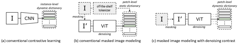
Figure 1: Conventional contrastive learning methods (e.g., MoCo (He et al., 2020), SimCLR (Chen et al., 2020)) and masked image modeling methods (e.g., BEiT (Bao et al., 2022), PeCo (Dong et al., 2021)) both perform the pretext task of vision dictionary look-up, where the superiority of the latter ones lie in the patch-level denoising auto-encoding mechanism to enable fine-grained visual context understanding of vision Transformers (Dosovitskiy et al., 2021). We introduce to cast masked image modeling as denoising contrastive learning to avoid the extra training stages of image tokenizer, rendering a flexible, simple and effective pre-training paradigm.

2 Related Work

Self-supervised learning via vision dictionary look-up.

The pretext task of contrastive learning (Chen et al., 2020; He et al., 2020; Caron et al., 2020) dominates self-supervised visual pre-training in the era of CNNs. Contrastive learning methods generally perform instance-level dictionary look-up. The anchors are pulled closer to their positive keys at the same time pushing away from the negative keys. The establishment of vision dictionaries is critical for the contrast regularization. For example, the seminal work MoCo (He et al., 2020) builds the vision dictionary with a first-in-first-out queue, driven by a momentum encoder. The concurrent work SimCLR (Chen et al., 2020) uses a large batch size to enlarge the dictionary with more negative keys. SwAV (Caron et al., 2020) further introduces an online clustering algorithm in an unsupervised manner, and the cluster assignments serve for the dictionary keys. Despite the great achievements with CNNs, these methods are gradually abandoned with the introduction of ViTs (Dosovitskiy et al., 2021) due to the lack of inductive bias, which requires stronger supervision for better pre-training performance.

Researchers attempt to reproduce the success of masked language modeling (Devlin et al., 2019) in self-supervised learning of ViTs via patch-level dictionary look-up. Specifically, BEiT (Bao et al., 2022) introduces a new pretext task, namely, masked image modeling, for visual pre-training. They tokenize high-dimensional images into discrete vision tokens by a discrete VAE (Ramesh et al., 2021) to establish a static patch-level dictionary as in NLP tasks. A proportion of image patches are randomly masked, the backbone network is then trained to recover the vision token ids of the masked patches, rendering a denoising mechanism. Follow-up works make efforts to further improve the static dictionaries, e.g., mc-BEiT (Li et al., 2022) introduces eased and refined dictionaries with multiple choices. PeCo (Dong et al., 2021) proposes to produce perceptual-aware keys in the patch-level dictionary. Though promising results, these methods all require extra training stages and even extra data for obtaining a proper image tokenizer.

We would also like to mention and thank the classic denoising auto-encoding methods (Vincent et al., 2010; Seung, 1997). Though they did not mask patches in Transformer, these pilot works on auto-encoding and emphasized reconstruction have well inspired the deep learning community.

Tokenizer-free masked image modeling (MIM) methods.

There are other recent works that cast MIM as a pixel-level reconstruction task (e.g., MAE (He et al., 2022)) or a self-distillation task (e.g., iBOT (Zhou et al., 2022)) rather than dictionary look-up. However, they fail to achieve competitive results using the same training epochs and perform especially unsatisfactorily on small-scale architectures due to the weak regression constraints (see Appendix B.4). Moreover, iBOT is not a pure MIM method as it heavily depends on the vanilla DINO (Caron et al., 2021) loss (i.e., the global self-distillation loss on [CLS] tokens). It actually conducts MIM on top of DINO and argues that MIM alone hardly captures visual semantics. However, we would like to clarify that it is actually due to the improper MIM constraints. Contrastive learning is proven to be good at structuring the visual space but does not been successfully employed in MIM before. We propose a flexible pure MIM method without extra dependencies, including offline tokenizer or global discrimination loss.

Dense contrast vs. denoising contrast.

There are some previous works on contrastive learning devoted to taking local feature representations into consideration, e.g., DenseCL (Wang et al., 2021). Though the form of InfoNCE (Van den Oord et al., 2018) is similar, they show significant differences from our ConMIM in both motivation and method design. They focus on how to learn better pre-trained weights for dense downstream tasks, e.g., object detection and segmentation, but hardly encourage the patch-level visual context reasoning as it is a contrastive-only task, showing inferior performance on ViT pre-training. Moreover, DenseCL depends on the global discrimination loss to ensure correct local correspondences and needs to carefully balance the global and local constraints. Such a chicken-and-egg problem can be seamlessly addressed in our well-designed denoising mechanism, including both the masking operation and the asymmetric designs. See Appendix B.4.1 for experimental comparisons. There are also some concurrent works (Tao et al., 2022; Huang et al., 2022) that study contrastive learning in MIM. ConMIM is conducted independently with them.

3 Preliminaries

The pretraining-and-then-finetuning paradigm has been proven to be effective for visual representation learning and various downstream tasks, where self-supervised pre-training is the most popular. Since there are no ground-truth annotations available, the design of pretext tasks is critical to the pre-training performance. Though driven by various motivations and progressing architectures (He et al., 2016; Dosovitskiy et al., 2021), the pretext task of visual self-supervised learning is essentially to perform vision dictionary look-up, inspired by the success of NLP tasks.

3.1 Contrastive Learning: Instance-level Vision Dictionary Look-up

From the perspective of vision dictionary look-up, prominent contrastive learning methods establish instance-level vision dictionaries via a fixed-length queue (He et al., 2020) or batch-wise samples (Chen et al., 2020). The keys in the dictionary are dynamically updated as pre-training proceeds. Given an image $x$, its feature representation is encoded by feeding it into the backbone network, i.e., $f(x)$. An InfoNCE loss (Van den Oord et al., 2018) is employed to regularize this representation, bringing it closer to its positive key $k_{+}$ while staying away from negative keys, denoted as

$$\mathcal{L}_{\rm con}(x)=-\log\frac{\exp{(\langle f(x),k_{+}\rangle/\tau)}}{\sum_{i=1}^{K}\exp{(\langle f(x),k_{i}\rangle/\tau)}},$$ (1)

where $\langle\cdot,\cdot\rangle$ is the cosine similarity measured by the dot product between two $L_{2}$-normalized features, $\tau$ is the temperature hyper-parameter, $k$ is the dynamic key, and $K$ is the dictionary size. Generally, the positive key is built by another view of the same instance (Tian et al., 2020), e.g., different image augmentations.

3.2 Masked Image Modeling: Patch-level Vision Dictionary Look-up

With the popularity of Transformer architectures (Dosovitskiy et al., 2021) in computer vision tasks, the pretext task of masked image modeling gradually dominates visual representation learning. It randomly masks a large percentage of image patches and trains the backbone network to recover the token ids of corrupted image via more fine-grained patch-level vision dictionary look-up. The dictionary is generally static and pre-defined by an off-the-shelf image tokenizer (Ramesh et al., 2021; Esser et al., 2021), which converts continuous visual signals into discrete keys. For example, in the seminal work BEiT (Bao et al., 2022), a pre-learned discrete VAE is adopted as the tokenizer. The masked patch prediction is then cast as a classification task with cross-entropy loss,

$$\mathcal{L}_{\rm mim}(x)=\mathbb{E}_{j\in\mathcal{M}}\left[-\log p(y_{j}|f(\hat{x})_{j})\right],$$ (2)

where $\mathcal{M}$ denotes the set of masked patch indices, $\hat{x}$ is the corrupted image after randomly masking, $y_{j}$ is the positive key index in the patch-level dictionary, and $p(\cdot|\cdot)$ indicates the probability that correctly identifies the recovered patch $f(\hat{x})_{j}$ with a patch index of $j$.

4 Masked Image Modeling with Denoising Contrast

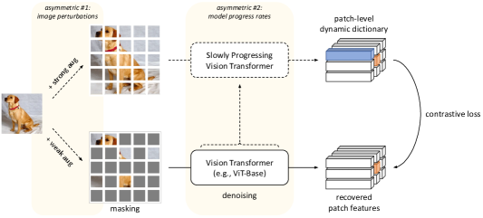
Figure 2: Our ConMIM performs the masked patch prediction with denoising contrast, coupling with two asymmetric designs to achieve state-of-the-art performance on self-supervised image pre-training. The slowly progressing vision Transformer is a snapshot of the backbone network under training, and we do not require any off-the-shelf image tokenizers. The training objective of denoising contrastive loss performs a patch-level look-up from dynamic vision dictionaries and enhances the network’s capability to capture more fine-grained visual context.

Despite that existing contrastive learning and masked image modeling methods optimize the backbone network towards different training objectives (i.e., InfoNCE loss and cross-entropy loss), they both attempt to learn discriminative visual representations via dictionary look-up. Two key factors lead to the state-of-the-art performance of masked image modeling. (1) More fine-grained supervision from instance-level to patch-level benefits the vision Transformer architecture known for its data-hungry properties. (2) The denoising auto-encoding mechanism, formed by the masking-and-then-predicting paradigm, encourages the capability of the backbone network to capture contextualized representations. Though promising results are achieved by existing masked image modeling methods (Bao et al., 2022; Li et al., 2022; He et al., 2022), they either require extra training stages to establish static vision dictionaries with offline image tokenizers or lack powerful MIM constraints.

To this end, we call for a revitalization of contrastive learning, which has good capability to structure the latent space for self-supervised representation learning. A new self-supervised pre-training method, ConMIM, is introduced to perform pure masked image modeling with denoising contrastive objectives while eliminating the dependence on pre-learned image tokenizers, as shown in Figure 2.

Patch-level dynamic dictionary.

We build dynamic patch-level dictionaries to form the learning targets for masked patch prediction on-the-fly. Specifically, during each training iteration, the full input image $x$ is fed into the backbone network to embed the patch feature representations, serving as keys in the dynamic dictionary, i.e., $\{f(x)_{i}|_{i=1}^{K}\}$ where $i$ is the patch index, $K$ is the dictionary size as well as the total number of patches within an image (e.g., $K=196$ keys for a $224\times 224$ image with a patch size of $16\times 16$). Without the loss of representation discriminativeness, we build separate dictionaries for each image, that is, only operate patch-level dictionary look-up within each image. We discuss this design in Sec. 5.4.2 with ablation studies using a larger or smaller dictionary size, where inferior results are achieved and require extra computational overhead.

Denoising contrastive objective.

The corrupted image, $\hat{x}$, is then fed into the backbone network, and we denote the encoded patch feature representation of a certain masked patch as $f(\hat{x})_{j},j\in\mathcal{M}$. The backbone network is trained to denoise the corrupted image and recover the masked patches through visual context reasoning. The masked patch recovery is regularized by a patch-level dictionary look-up in the form of an InfoNCE loss (Van den Oord et al., 2018),

$$\mathcal{L}_{\rm conmim}(x)=\mathbb{E}_{j\in\mathcal{M}}\left[-\log\frac{\exp{(\langle f(\hat{x})_{j},{\rm sg}[f(x)_{j}]\rangle/\tau)}}{\sum_{i=1}^{K}\exp{(\langle f(\hat{x})_{j},{\rm sg}[f(x)_{i}]\rangle/\tau)}}\right],$$ (3)

where ${\rm sg}[\cdot]$ indicates stop-gradient operation. We only backpropagate the gradients of the corrupted inputs $f(\hat{x})$ because backpropagating the gradients of the full input $f(x)$ may lead to information leakage and useless denoising. With the above training objectives, the backbone network is encouraged to better capture the visual context and learns to encode local discriminative representations.

Asymmetric design.

As patches (e.g., $16\times 16$) are small-scale inputs with less useful information and highly redundant semantics, we need to make the pre-training task more challenging to improve the backbone network. Towards this goal, the recent work MAE (He et al., 2022) proposes to mask a large proportion of patches. In our work, besides the large proportion of patch dropout, we further introduce two asymmetric designs to enable a stronger denoising regularization during pre-training.

(1) Asymmetric image perturbations. We adopt different data augmentations for the full input image $x$ and the corrupted image $\hat{x}$ before feeding into the backbone network. To be specific, we utilize stronger augmentations for the full input image referring to contrastive learning methods (Chen et al., 2020), including random flip, resize, crop, color distort, Gaussian blur, and solarization. And we only use basic augmentations for the corrupted image referring to masked image modeling methods (Bao et al., 2022), including random flip, resize, and crop. Note that we use the same flip, resize and crop operations for paired inputs in order to keep the patch positions consistent. We discuss the alternative options in Sec. 5.4.3. We observe that it is sub-optimal to use strong augmentations for corrupted images, and the reason might be the too difficult pretext task to regularize, i.e., the backbone network needs to recover the strong-augmented corrupted input towards the full input targets with asymmetric perturbations.

(2) Asymmetric model progress rates. We employ different model progress rates of the backbone network for embedding the corrupted input and full input to avoid information leakage. We use the in-training network i.e., the one optimized by loss backpropagation for the corrupted input while using its momentum updated version for the full input. The momentum encoder (He et al., 2020) is known as a slowly progressing model that can encode more challenging but semantically consistent key feature representations for building dictionaries. Specifically, we denote the model parameters of the backbone $f(\cdot)$ as $\theta$ and the model parameters of the momentum updated one as $\tilde{\theta}$. The momentum encoder is updated via $\tilde{\theta}=(1-\alpha)\theta+\alpha\tilde{\theta}$ in each iteration, where $\alpha\in[0,1]$ is the momentum coefficient. Larger coefficients indicate slower model progress.

Pre-training setup.

ConMIM pre-training is conducted on the training set of ImageNet-1K (Deng et al., 2009) dataset in a self-supervised manner. We utilize ViT-S/16, ViT-B/16 and ViT-L/16 (Dosovitskiy et al., 2021) as the backbone networks. Following MoCo v3 (Chen* et al., 2021), we use a 3-layer projection head on top of the backbone network for pre-training and discard it when transferring to downstream tasks. The input images are all resized to $224\times 224$ and the patch size is set to $16\times 16$. We follow the masking strategy of MAE (He et al., 2022), i.e., 75% patches are randomly masked. The learning rate is set to 5e-4, with a warmup of 10 epochs, and cosine learning rate decay. The temperature $\tau$ is set to 0.1 and the momentum coefficient $\alpha$ is initially set to 0.996 with a cosine scheduler. ViT-B/16 and ViT-L/16 are pre-trained for 800 epochs in total and ViT-S/16 is pre-trained for 300 epochs if not specified. The other hyper-parameters are mostly the same as BEiT (Bao et al., 2022). More implementation details can be found in Appendix A.

5 Experiments

We evaluate the models pre-trained by our ConMIM on different downstream tasks, including image classification on ImageNet-1K (Deng et al., 2009) (Sec. 5.1), semantic segmentation on ADE20K (Zhou et al., 2017) (Sec. 5.2), object detection and instance segmentation on COCO (Lin et al., 2014) (Sec. 5.3). We further discuss the key components in ConMIM pre-training via ablation studies in Sec. 5.4, the scalability on larger dataset in Sec. 5.5, and the running time in Sec. 5.6. Hyper-parameter details can be found in Appendix A.1 and analysis in Appendix B.1.

5.1 Image Classification

Method	Arch.	#Epochs	Acc.
scratch	ViT-B/16	-	81.8
MoCo v3	ViT-B/16	600	83.2
DINO	ViT-B/16	1600	82.8
BEiT	ViT-B/16	300	82.9
ConMIM	ViT-B/16	300	83.5
iBOT	ViT-B/16	600	82.0
BEiT	ViT-B/16	800	83.2
MAE	ViT-B/16	800	83.3
ConMIM	ViT-B/16	800	83.7
SimMIM	ViT-B/16	800	83.8
MAE	ViT-B/16	1600	83.6
iBOT	ViT-B/16	1600	84.0
scratch†	ViT-B/16	-	83.1
BEiT†	ViT-B/16	800	84.6
ConMIM†	ViT-B/16	800	85.3
MAE†	ViT-B/16	1600	84.9
iBOT†	ViT-B/16	1600	85.0

Table 1: Top-1 accuracy (%) on ImageNet-1K (Deng et al., 2009) classification using ViT-Base (Dosovitskiy et al., 2021). All the models use only ImageNet-1K with a resolution of $224^{2}$ for pre-training. (^†) The resolution of $384^{2}$ is used for fine-tuning. We follow the same $384^{2}$ fine-tuning setup of BEiT (Bao et al., 2022), i.e., after fine-tuning with $224^{2}$, another 10% epochs are further used for fine-tuning on $384^{2}$.

Method	Arch.	#Epochs	Acc.
scratch	ViT-S/16	-	79.8
MoCo v3	ViT-S/16	600	81.4
DINO	ViT-S/16	1600	81.5
BEiT	ViT-S/16	300	81.3
ConMIM	ViT-S/16	300	82.0
iBOT	ViT-S/16	600	81.5
SimMIM	ViT-S/16	800	80.1
MAE	ViT-S/16	800	80.9
iBOT	ViT-S/16	3200	82.3
ConMIM†	ViT-S/16	300	83.9

Table 2: Top-1 accuracy (%) on ImageNet-1K classification using ViT-Small.

Method	Arch.	#Epochs	Acc.
scratch	ViT-L/16	-	82.6
MoCo v3	ViT-L/16	600	84.1
MAE	ViT-L/16	400	84.3
ConMIM	ViT-L/16	400	84.6
BEiT	ViT-L/16	800	85.2
MAE	ViT-L/16	800	85.2
ConMIM	ViT-L/16	800	85.2
iBOT	ViT-L/16	1000	84.8
ConMIM	ViT-L/16	1600	85.5
MAE	ViT-L/16	1600	85.9
BEiT†	ViT-L/16	800	86.3
ConMIM†	ViT-L/16	800	86.3
ConMIM†	ViT-L/16	1600	86.5

Table 3: Top-1 accuracy (%) on ImageNet-1K classification using ViT-Large.

We test our ConMIM by fine-tuning the pre-trained models on ImageNet-1K (Deng et al., 2009) classification, which contains 1.3M images out of 1K classes in total. We mostly follow the fine-tuning setup of BEiT (Bao et al., 2022). To be specific, we use 100 epochs with a warm-up of 20 epochs, and a layer decay of 0.65 for ViT-Base fine-tuning. 200 epochs with a warm-up of 5 epochs and a layer decay of 0.8 for ViT-Small fine-tuning. 50 epochs with a warm-up of 5 epochs and a layer decay of 0.75 for ViT-Large fine-tuning. We illustrate the evaluation results in Tables 3,3,3. We observe that models with pre-trained weights overwhelmingly outperform the ones trained from scratch by DeiT (Touvron et al., 2021), demonstrating the significance of self-supervised visual representation learning. Compared to the pioneering work of masked image modeling, BEiT (Bao et al., 2022), we consistently outperform it when fine-tuning on ViT-Base and ViT-Small models with both image resolutions of $224\times 224$ and $384\times 384$. Moreover, we do not require any extra tokenizing networks as in BEiT, realizing more efficient and flexible one-stage pre-training. MAE (He et al., 2022) and iBOT (Zhou et al., 2022) cast masked image modeling as reconstruction or distillation tasks rather than vision dictionary look-up. As we discussed before, they require more training epochs for optimal performance as the regularization of regression loss is much more eased than the contrastive loss. Such flaws are especially evident in the performance of small-scale models.

5.2 Semantic Segmentation

Methods	Arch.	#Ep.	mIOU
BEiT‡	ViT-S/16	300	46.3
ConMIM‡	ViT-S/16	300	47.7
scratch	ViT-B/16	-	45.3
MoCo v3	ViT-B/16	600	47.2
BEiT	ViT-B/16	800	45.6
ConMIM	ViT-B/16	800	46.0
DINO	ViT-B/16	1600	46.8
MAE	ViT-B/16	1600	48.1
iBOT	ViT-B/16	1600	50.0
BEiT‡	ViT-B/16	800	47.7
ConMIM‡	ViT-B/16	800	49.8
MAE‡	ViT-B/16	1600	48.0
scratch	ViT-L/16	-	49.9
MoCo v3	ViT-L/16	600	49.1
BEiT‡	ViT-L/16	800	53.3
ConMIM‡	ViT-L/16	800	53.7
MAE	ViT-L/16	1600	53.6

Table 4: Semantic segmentation on ADE20K (Zhou et al., 2017) in terms of mIOU (%). “#Ep.” means the number of pre-trained epochs. (^‡) Transferring after intermediate fine-tuning on ImageNet-1K (Deng et al., 2009), which is a common practice of BERT (Devlin et al., 2019).

Methods	Arch.	#Ep.	APbox	APmask
scratch	ViT-S/16	-	43.1	38.8
MAE	ViT-S/16	800	38.9	35.6
ConMIM‡	ViT-S/16	300	45.8	41.0
MAE‡	ViT-S/16	800	41.5	37.8
SimMIM‡	ViT-S/16	800	43.0	38.7
scratch	ViT-B/16	-	46.5	41.7
MoCo v3	ViT-B/16	600	47.3	42.2
BEiT	ViT-B/16	800	47.4	42.1
ConMIM	ViT-B/16	800	47.8	42.5
SimMIM	ViT-B/16	800	48.7	43.2
DINO	ViT-B/16	1600	47.6	42.3
iBOT	ViT-B/16	1600	48.3	42.7
MAE	ViT-B/16	1600	48.0	43.0
BEiT‡	ViT-B/16	800	48.2	43.3
SimMIM‡	ViT-B/16	800	48.4	43.5
ConMIM‡	ViT-B/16	800	48.7	43.6
MAE‡	ViT-B/16	1600	47.8	42.9

Table 5: Object detection and instance segmentation on COCO (Lin et al., 2014) in terms of AP^box (%) and AP^mask (%). We tune the optimal learning rate for each model following (He et al., 2022). (^‡) With intermediate fine-tuning on ImageNet.

We evaluate ConMIM on the downstream semantic segmentation using ADE20K (Zhou et al., 2017) benchmark, which consists of 25K images of 150 semantic categories. We use the evaluation metric, mean intersection over union (mIOU), for reference. We use UperNet (Xiao et al., 2018) and adopt the same setup as BEiT (Bao et al., 2022). Images are resized to $512\times 512$ as input, and the model is fine-tuned for 160K iterations in total. We also use intermediate fine-tuning to fully exploit the potential of the pre-trained models following BEiT (Bao et al., 2022), i.e., first fine-tuning the pre-trained models on ImageNet-1K classification and then transferring to ADE20K. The results are shown in Table 5. We consistently surpass the baseline BEiT with significant improvements, e.g., our 49.8% vs. BEiT’s 47.7% on ViT-Base. Moreover, our ConMIM using ViT-Small even achieves comparable performance with BEiT using ViT-Base, i.e., 47.7%. Models pre-trained by masked image modeling generally achieve better performance on segmentation than the ones pre-trained by conventional contrastive learning, e.g., MoCo v3 (Chen* et al., 2021).

5.3 Object Detection and Instance Segmentation

For object detection and instance segmentation, we fine-tune Mask R-CNN (He et al., 2017) end-to-end on COCO (Lin et al., 2014). We follow the implementation of (Li et al., 2021) and reproduce all the results in Table 5 since (Li et al., 2021) is still close-source. To tame quadratic complexity with self-attention, most attention blocks in the ViT backbone are replaced with windowed blocks except for four global blocks to perform cross-window interaction. Four up/down-sample modules are evenly placed with ViT to produce pyramid features required by FPN (Lin et al., 2017). The training recipes keep the same with (Li et al., 2021). An input image is resized to $1024\times 1024$ and augmented by large scale jitter (Ghiasi et al., 2021), with a resize scale of [0.1, 2.0]. We fine-tune the pre-trained models for 25 epochs using an AdamW (Loshchilov & Hutter, 2017) optimizer with a weight decay of 0.1 and cosine learning rate scheduler. All experiments are performed under the same settings, except for the learning rate is specifically tuned for each model, which strictly follows (He et al., 2022) in order to keep fair comparisons as it exploits the potential of each pre-trained method. We achieve much better performance than MAE (He et al., 2022) on ViT-Small.

5.4 Ablation Studies

We discuss component design in ConMIM through ablation studies. All the experiments in this section are conducted using ViT-B/16 (Dosovitskiy et al., 2021) pre-trained for 300 epochs, and we report the top-1 classification accuracy after fine-tuning on ImageNet-1K (Deng et al., 2009).

5.4.1 Analysis of Denoising Auto-encoding Mechanism

Models	ImageNet Acc.
DeiT-B (training from scratch)	81.8
MoCo v3 (conventional contrastive learning)	83.2
ConMIM (Ours)	83.51
denoising patch-level contrast $\rightarrow$ vanilla instance-level contrast	82.26 (-1.25%)
denoising patch-level contrast $\rightarrow$ vanilla patch-level contrast	fail

Table 6: Ablation studies on the effect of denoising auto-encoding mechanism.

The denoising auto-encoding mechanism is critical to the success of masked image modeling, where the fine-grained patch-level supervision and the masking-and-the-predicting paradigm are the two key factors. We conduct ablation studies in Table 6 to analyze their effect. (1) We remove the entire denoising auto-encoding mechanism from ConMIM, i.e., using average local tokens to perform vanilla instance-level contrastive loss, significant performance drops (-1.25%) are observed. Such a result is even worse than MoCo v3 (Chen* et al., 2021), the state-of-the-art method for conventional contrastive learning. See the visualization in Appendix B.2 for more intuitive comparisons. (2) When only discarding the masking strategy while keeping patch-level contrast, the experiment totally fails due to the trivial information leakage with semantically repetitive patches.

5.4.2 Analysis of Patch-level Dynamic Dictionary

Models	ImageNet Acc.
DeiT-B (training from scratch)	81.8
ConMIM (Ours)	83.51
more: intra-image negative keys $\rightarrow$ intra-gpu negative keys	82.60 (-0.91%)
fewer: intra-image negative keys $\rightarrow$ filtered intra-image negative keys	83.12 (-0.39%)

Table 7: Ablation studies on the dictionary size of ConMIM.

ConMIM performs masked image modeling towards the objective of an intra-image inter-patch contrastive loss, i.e., the dictionary is built individually for each image. The size of the dictionary has effects on the regularization of negative keys. We discuss such a design by either expanding the dictionary or reducing it, as shown in Table 7. (1) We expand the dictionary by gathering other images’ keys on the same GPU. Performance drops are observed. The reason might be that the keys from the same image share similar domains and serve as hard negatives for each other. Gathering more negatives from other domains actually ease the regularization. (2) Although patches within the same images can act as hard negatives, they might also be noisy negatives as patches are highly semantically redundant, e.g., patches from different positions may carry similar patterns. So we try to filter them by excluding negative keys that are highly similar to the anchor patch in the latent space. Slight accuracy decreases are shown, indicating that we may exclude some valuable hard negatives. We acknowledge that, although ConMIM can achieve the state-of-the-art results to date, there should be room for further refinement in dictionary design. Further studies are called for.

5.4.3 Analysis of Asymmetric Designs

Models	ImageNet Acc.
DeiT-B (training from scratch)	81.8
ConMIM (Ours)	83.51
w/o asymmetric image perturbations, use stronger one	83.41 (-0.10%)
w/o asymmetric image perturbations, use basic one	83.35 (-0.16%)
w/ asymmetric image perturbations but switch	82.62 (-0.89%)
w/o asymmetric model progress rates	81.53 (-1.98%)

Table 8: Ablation studies on the effect of asymmetric designs.

We introduce two asymmetric designs in ConMIM to enable a stronger denoising auto-encoding mechanism during pre-training. We discuss their effects in Table 8. (1) Asymmetric image perturbations. We use a stronger augmentation for the full input while the basic one for the corrupted image in ConMIM. We try to remove such asymmetric augmentation design and find slight performance drops when using either the stronger one or the basic one for both inputs. More significant performance drops can be observed when directly switching their augmentations. We draw a seemingly counterintuitive conclusion versus conventional contrastive learning. However, it is actually consistent with the theoretical analysis in (Wang et al., 2022b) that the in-training (source) network of contrastive learning requires high variance of input distribution, where the masking strategy already introduces much higher variance than the full input for the momentum (target) network. Further applying stronger augmentation for the corrupted input may lead to a too difficult pretraining task for the network to regularize, similar to the findings in MAE (He et al., 2022). (2) Asymmetric model progress rates. We use a slowly progressing momentum model of the backbone network to embed more challenging but semantically consistent key representations. Such a design is important to avoid information leakage caused by feeding the full input (target) into the same model. When removing it, noticeable accuracy decreases are shown, i.e., -1.98%, even worse than DeiT baseline.

5.5 Uncurated Pre-training Data

We would like to see if ConMIM scales well to larger uncurated datasets. Referring to SLIP (Mu et al., 2021), we pre-train on YFCC15M (Thomee et al., 2016), which is about 12 times larger than ImageNet-1k. See the results below in Table 9, ConMIM surpasses both SLIP (using language supervision) and MAE (a comparable pure MIM method) on ViT-B/16, further verifying the effectiveness and scalability of our ConMIM in real-world applications.

Method	Arch.	#Epochs (YFCC15M)	ImageNet Acc.
SLIP	ViT-B/16	50	82.9%
MAE	ViT-B/16	40	83.0%
ConMIM	ViT-B/16	40	83.3%

Table 9: Scalability on larger uncurated data.

5.6 Running Time

We measure the running time per epoch based on the anchor BEiT (Bao et al., 2022) in Table 10. BEiT requires an additional tokenizer (Ramesh et al., 2021), whose training time is not included here. Note that iBOT (2-view) needs to switch two views and four forward passes in total, and BEiT and ConMIM are 1-view method without switching. MAE is more efficient but achieves inferior performance than our ConMIM. Considering the effectiveness and flexibility, a slightly increasing time over BEiT is acceptable.

Method	Setup	Time per epoch
MAE	1-view, 1-pass	0.35$\times$
BEiT	1-view, 2-pass	1.0$\times$ (w/ extra tokenizer)
ConMIM	1-view, 2-pass	1.05$\times$
iBOT	2-view, 4-pass	1.40$\times$
iBOT (default)	(2+10)-view, 14-pass	2.15$\times$

Table 10: Running time statistics.

6 Conclusion and Discussion

We first propose to perform masked image modeling (MIM) with denoising contrast, a simple and flexible pure MIM method with advanced downstream performance. Besides the technical contribution, we would like to emphasize our intriguing insights and potential broader impacts. We are the first to indicate that MIM and contrastive learning both essentially perform vision dictionary look-up and analyze the key factors that make MIM more effective on ViTs, i.e., the fine-grained patch-level constraints and denoising auto-encoding mechanism. More importantly, we hope our work, revitalizing contrastive learning when MIM dominates, would well motivate the community to conduct an objective and comprehensive study of two lines of pre-training methods, and further inspire NLP and multimodal research. Reproducibility is declared in Appendix A, more experimental results in Appendix B, and limitations in Appendix C.

Appendix A Reproducibility

We adopt 16 A100 GPUs for pre-training (32 A100 GPUs for ViT-L/16). ViT-S/16 requires less than 1 day for 300 epochs, ViT-B/16 requires around 3 days for 800 epochs and ViT-L/16 requires around 5 days for 800 epochs. A fluctuation within $\pm$0.1% accuracy may be observed on classification when pre-training multiple times with distinct random seeds (use 0 in default).

A.1 Hyper-parameters

Configuration	ViT-S/16	ViT-B/16	ViT-L/16
Layers	12	12	24
Hidden size	384	768	1024
Attention heads	6	12	16
Attention head size	64
Patch size	$16\times 16$
Training epochs	300	800	800
Batch size	2048
Adam $\epsilon$	1e-8
Adam $\beta$	(0.9, 0.98)
Peak learning rate	5e-4
Minimal learning rate	1e-5
Learning rate schedule	Cosine
Warmup epochs	10
Initial momentum coefficient $\alpha$	0.996
Maximal momentum coefficient $\alpha$	1
Momentum coefficient schedule	Cosine
Temperature $\tau$	0.1
Stoch. depth	0.1	None	None
Gradient clipping	3	3	1
Dropout	None
Weight decay	0.05
Masking patch size	16	32	32
Basic Data Augment	RandomResizeAndCrop
Strong Data Augment	ColorJitter(0.4,0.4,0.2,0.1), GaussianBlur(0.1), Solarization(0.2)
Input resolution	$224\times 224$

Table 11: Hyper-parameters for ConMIM pre-training on ImageNet-1K.

Configuration	ViT-S/16	ViT-B/16	ViT-L/16
Peak learning rate	{1e-3,2e-3,3e-3,4e-3,5e-3}
Batch size	1024
Fine-tuning epochs	200	100	50
Warmup epochs	5	20	5
Layer-wise learning rate decay	0.8	0.65	0.75
Adam $\epsilon$	1e-8
Adam $\beta$	(0.9, 0.999)
Minimal learning rate	1e-6
Learning rate schedule	Cosine
Repeated Aug	None
Weight decay	0.05
Label smoothing	0.1
Dropout	None
Gradient clipping	None
Stoch. depth	0.1	0.1	0.2
Erasing prob.	0.25
Input resolution	$224\times 224$ or $384\times 384$
Rand Augment	9/0.5
Mixup prob.	0.8
Cutmix prob.	1.0
Color jitter	0.4

Table 12: Hyper-parameters for fine-tuning ConMIM on ImageNet-1K classification.

Configuration	ViT-S/16	ViT-B/16	ViT-L/16
Peaking learning rate	{1e-5,3e-5,5e-5,7e-5}
Fine-tuning steps	160K
Batch size	16
Adam $\epsilon$	1e-8
Adam $\beta$	(0.9, 0.999)
Layer-wise learning rate decay	0.9	0.9	0.95
Minimal learning rate	0
Learning rate schedule	Linear
Warmup steps	1500
Dropout	None
Stoch. depth	0.1
Weight decay	0.05
Input resolution	$512\times 512$
Position embedding	Relative
Position embedding interpolate	Bilinear

Table 13: Hyper-parameters for fine-tuning ConMIM on ADE20K semantic segmentation.

Configuration	ViT-S/16	ViT-B/16
Fine-tuning epochs	25
Peaking learning rate	1e-4
Learning rate decay	cosine
Adam $\epsilon$	1e-8
Adam $\beta$	(0.9, 0.999)
Dropout	None
Stoch. depth	0.1
Weight decay	0.1
Batch size	64
Input size	$1024\times 1024$
Position embedding	Abs. + Rel.
Augmentation	LSJ(0.1, 2.0)

Table 14: Hyper-parameters for fine-tuning ConMIM on COCO object detection and instance segmentation.

A.2 Pseudocode

Algorithm 1 Pseudocode of ConMIM pre-training in a PyTorch-like style.

⬇

# f: backbone encoder, e.g., vit-base model

# t: temperature, \tau in the paper

# m: momentum, \alpha in the paper

f_slow.params = f.params # initialize

for (x, mask) in loader: # load a mini-batch x with N samples

# image preprocess with asymmetric perturbations

x = aug_basic(x) # share same basic aug for paired inputs

x_full = aug_strong(x)

x_corrupted = x*(1-mask)+mask_token.expand_as(x)*mask # randomly mask 75% patches

# build patch-level dynamic dictionaries with asymmetric models

with torch.no_grad():

keys = f_slow(x_full) # NxKxD, K is the number of patches

feats = f(x_corrupted) # NxKxD

# dictionary look-up with denoising contrastive loss (Eq.(3))

sim = bmm(feats.view(N,K,D), keys.view(N,D,K)).view(-1,K) # (NxK)xK

labels = range(K).repeat(N) # (NxK)

mask = mask.view(-1) # (NxK)

loss = CrossEntropyLoss(sim[mask]/t, labels[mask])

# update model

loss.backward()

update(f.params)

f_slow.params = (1-m)*f.params+m*f_slow.params

 bmm: batch matrix multiplication

Appendix B Experiments (Cont.)

B.1 Hyper-parameter Analysis

Strategy	Ratio	Acc.
Block	40%	82.12
	60%	83.20
	75%	83.11
	90%	82.63
Random	60%	82.52
	75%	83.51
	90%	83.04

Table 15: Discuss different masking strategies and ratios.

temperature $\tau$	Acc.
0.05	82.55
0.07	83.03
0.1	83.51
0.15	83.32
0.2	83.35

Table 16: Discuss temperature hyper-parameter in denoising contrastive loss.

momentum $\alpha$	Acc.
0.99	83.11
0.996	83.51
0.999	83.31

Table 17: Discuss momentum coefficient in the slowly progressing model.

Masking ratio.

The fine-tuning results on ImageNet using different masking strategies and ratios are shown in Table 17. Randomly masking at a ratio of 75% achieves the optimal performance.

Temperature.

We discuss the effect of temperature hyper-parameter in our denoising contrastive loss (Eq. (3)), as illustrated in Table 17. $\tau=0.1$ achieves the optimal performance empirically. We use this setup for both ViT-Small and ViT-Base.

Momentum.

The fine-tuning accuracy on ImageNet using our ConMIM with different values of initial momentum coefficient is shown in Table 17. ConMIM is actually not sensitive to this hyper-parameter and we adopt 0.996 in all experiments for optimal performance.

B.2 Visualizations

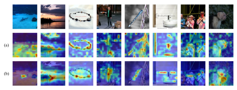
Figure 3: Visualize the self-attention map between [CLS] token and local tokens of the pre-trained ViT-B/16 (Dosovitskiy et al., 2021) model on ImageNet-1K (Deng et al., 2009), where (a) indicates ConMIM pretraining and (b) indicates the vanilla instance-level contrastive pre-training. Self-attention maps out of 12 attention heads are averaged. It can be observed that ConMIM-pretrained models are much more locally discriminative and aware of the visual context.

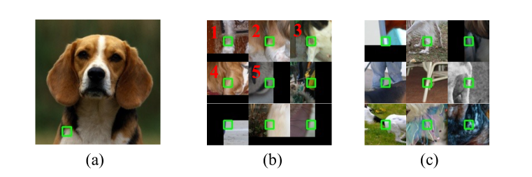
Figure 4: Visualize the dynamic dictionary composed of patches. The dictionary in ConMIM properly provides positive keys with similar semantics while the baseline tokenizer is vulnerable to various low-level changes. (a) The query patch from ImageNet validation set. (b) Top-ranked patches retrieved by ConMIM-pretrained model. (c) Patches out of the same ID (#1813) tokenized by dVAE (Ramesh et al., 2021) in baseline BEiT (Bao et al., 2022).

B.3 Partial Fine-tuning

Linear probing is inapplicable to evaluate pure MIM methods which are not designed towards linearly separable instance features. MIM pre-training aims to pursue better pre-trained weights and strong but non-linear features that complement downstream tasks. Linear probing fails to properly measure such properties according to MAE (He et al., 2022) and is also abandoned by BEiT (Bao et al., 2022). For a more comprehensive evaluation, we study partial fine-tuning (a middle ground between linear probing and fully fine-tuning) on ConMIM. As illustrated in Figure 5, fine-tuning a few blocks can achieve accuracy close to full fine-tuning.

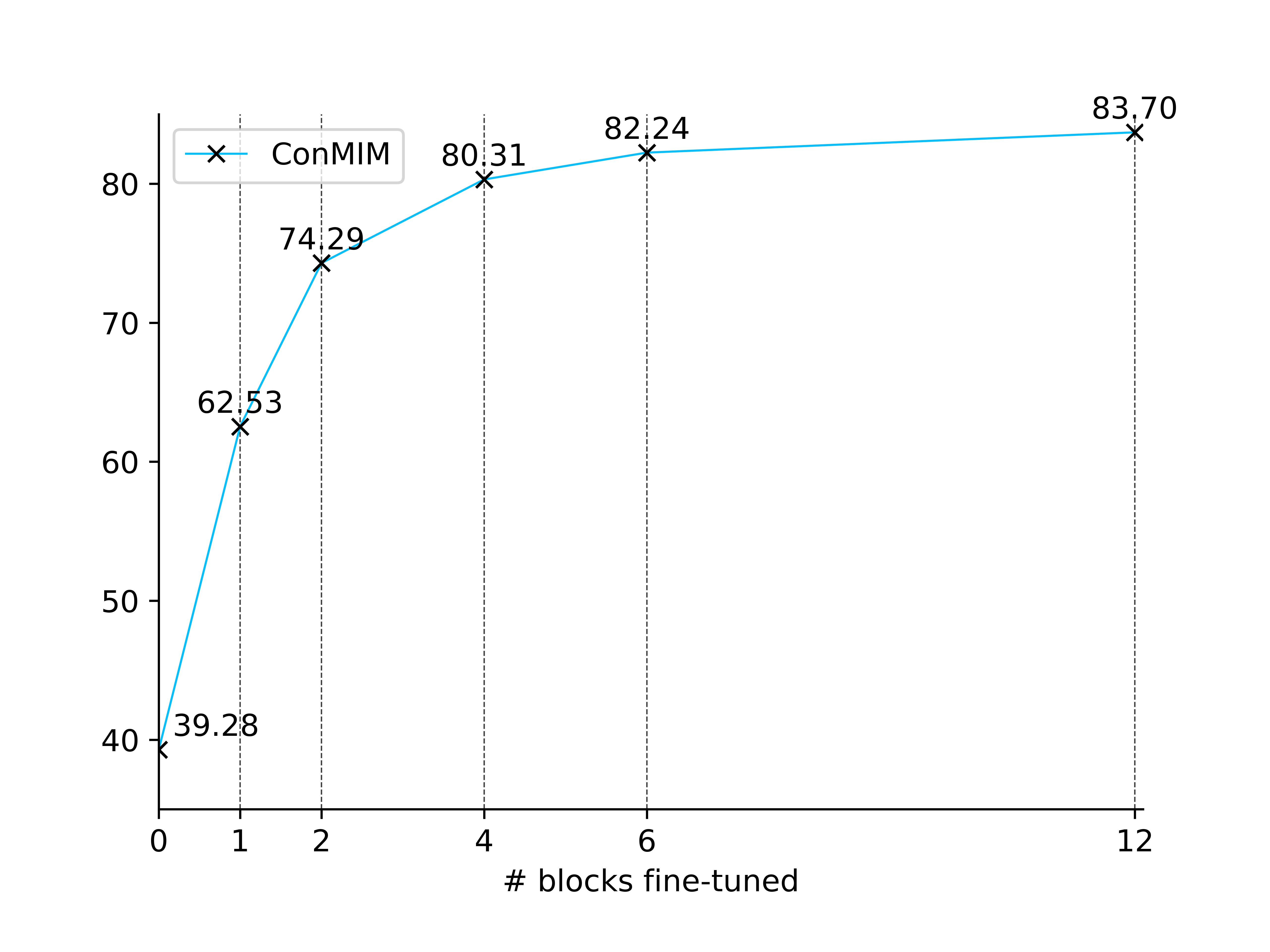
Figure 5: Partial fine-tuning of ConMIM-pretrained ViT-B/16 model.

B.4 Discussion with Related Works

B.4.1 Compare to iBOT and DenseCL

Method	#Views	# Pretrain Epochs	ViT-S/16	ViT-B/16
iBOT	2	300	81.5	82.0
DenseCL	1	300	81.4	81.9
ConMIM	1	300	82.0	83.5

Table 18: System-level comparison with iBOT (Zhou et al., 2022) and DenseCL (Wang et al., 2021). The results are reported on ImageNet-1K classification in terms of top-1 accuracy (%). iBOT switches 2 standard views for double loss calculating while ConMIM does not.

As iBOT (Zhou et al., 2022) is also a tokenizer-free method, someone considers ConMIM a variant of iBOT with DenseCL (Wang et al., 2021) loss. We would like to clarify that our ConMIM develops more proper constraints for pure MIM rather than a trivial combination of iBOT and DenseCL, motivated as follows.

Although iBOT abandons the offline tokenizer, it heavily depends on the vanilla DINO loss (i.e., the global self-distillation loss on [CLS] tokens). It actually conducts MIM on top of DINO and fails without the vanilla DINO loss. As an evidence, in Tab. 9 of iBOT’s original paper, the fine-tuning accuracy of ViT-S/16 significantly degrades from 81.5% to 79.4% (DeiT-S achieves 79.8%) when removing the vanilla DINO loss. iBOT paper argues that MIM alone hardly captures visual semantics. However, we would like to claim that it is mainly due to the weak patch-level self-distillation loss as MIM constraints in iBOT rather than the issue of pure MIM.

Compared to the regression regularization in self-distillation loss, contrastive learning is proven to be good at structuring the visual space, e.g., MoCo v3 (83.2%, 600ep) beats DINO (82.8%, 1600ep) on ViT-B/16. It is natural to exploit contrastive learning in a pure MIM pretraining method for capturing discriminative visual semantics, but unfortunately, it has never been explored before. We are the first to study it, and introduce a simple and flexible pure MIM method without extra dependencies (e.g., offline tokenizer or global discrimination loss).

DenseCL shows significant differences from our ConMIM in both motivation and method design except for the form of infoNCE (note that infoNCE is widely used for distinct purposes). DenseCL still depends on the global discrimination loss to ensure correct local correspondences and needs to carefully balance the global and local constraints (see Sec. 3.4 of its original paper). Such a chicken-and-egg problem can be seamlessly addressed in our denoising mechanism, including both the masking operation and the asymmetric designs. Moreover, DenseCL hardly encourages the patch-level visual context reasoning as it is a contrastive-only task.

We further provide system-level comparisons in Table 18. For a fair comparison, we retrain iBOT without multi-crop augmentation (but keeping 2 views) using its official code and re-implement DenseCL on ViT architectures. Our ConMIM achieves the optimal performance on both ViT-S/16 and ViT-B/16 architectures.

B.4.2 Compare to MAE

MAE is a pure MIM method without tokenizer. It casts masked image modeling as a per-pixel denoising reconstruction task with an $\ell_{1}$ regression loss. The contrastive constraints in ConMIM provide stronger semantic structured regularization than the pixel-level reconstruction loss in MAE, leading to better results with fewer epochs. Moreover, ConMIM is effective especially on small-scale architectures, e.g., ViT-S/16, indicating the necessity of good visual semantic structured constraints on less powerful models. The experimental comparisons are found in Table 19. MAE is trained for 1600 epochs in default and we retrain it using its official code for 800 epochs.

Method	Arch.	# Pretrain Epochs	Acc.
MAE	ViT-S/16	800	80.9
ConMIM	ViT-S/16	300	82.0
MAE	ViT-B/16	800	83.3
ConMIM	ViT-B/16	800	83.7

Table 19: Compare to MAE (He et al., 2022). The results are reported on ImageNet-1K classification in terms of top-1 accuracy (%). Also see the comparison on YFCC15M in Sec. 5.5 of main paper.

B.5 Analysis of Key Components

Aug. for corrupted image	Aug. for full image	BEiT	ConMIM
weak	weak	82.9 (default)	83.4
strong	strong	82.9	83.4
strong	weak	82.7	82.6
weak	strong	82.9	83.5 (default)

Table 20: Analysis of asymmetric perturbations using ViT-B/16 pre-trained for 300 epochs. The results are reported on ImageNet-1K classification in terms of top-1 accuracy (%). We observe a similar trend within two methods. Using symmetric perturbations for two views (weak*2 or strong*2) receives identical results within each method, which makes sense as the degree of perturbations for denoising doesn’t change. We use asymmetric perturbations to strengthen the denoising mechanism in ConMIM, however, the optimal setup “weak+strong” for ConMIM doesn’t work on BEiT since the full image encoder in BEiT is a fixed dVAE, which has certain robustness without training.

On the importance of each component.

There are three main components in ConMIM: denoising contrastive loss, asymmetric image perturbations, and asymmetric model progress rates. (a) When changing denoising contrastive loss to conventional BEiT loss (classification over token ids), the design of asymmetric image perturbations does not work anymore (see Table 20), and the design of asymmetric model progress rates is inapplicable since the full image encoder in BEiT is a fixed dVAE rather than an in-training network. (b) When changing asymmetric image perturbations into symmetric ones at the same time keeping the other two components consistent, slight performance drops are found with either strong or weak symmetric perturbations. Though the performance is not optimal, the pretraining is still valid as it outperforms DeiT (training from scratch). See Table 8 of our main paper. (c) When abandoning asymmetric model progress rates, the pre-training does not work since the results are even worse than DeiT. The reason might be the shortcut reconstruction with the information leakage. See Table 8 of our main paper.

To conclude, the importance ranking of the three components is denoising contrastive loss $>$ asymmetric model progress rates $>$ asymmetric image perturbations. The denoising contrast is our main method and the asymmetric model progress rates make it works. The asymmetric image perturbations bring extra gains.

Intuitions of component design.

As analyzed in (Xie et al., 2022), the pretraining task of masked image modeling encourages diverse attention learning in all layers of the Transformer architecture, and introduces locality inductive bias into the patch level. Such properties can also be considered as improving the patch/local uniformity, whereas the contrastive objectives are proven to be good at it (Wang & Isola, 2020). Intuitively, the training objective “per-patch (8192-class) classification in BEiT vs. per-patch contrastive in ConMIM” is similar to conventional “1000-class classification in ImageNet supervised pretraining vs. instance-level contrastive in self-supervised pretraining”. In short, we properly reformulate the MIM task with contrastive objectives to enhance diverse attention in vision Transformers with improved uniformity of patch distributions. As for the asymmetric components, (Wang et al., 2022b) demonstrates that the source network (in-training network updated by loss backpropagation) favors stronger perturbations that introduce high variance into the data distribution. The masking strategy introduces much higher variance than the full input for the momentum (target) network, corroborating the theoretical analysis in (Wang et al., 2022b).

Appendix C Limitations

The current version of ConMIM has the following limitations. (1) The intra-image inter-patch contrastive loss may carry some noise as there may exist semantically repetitive patches. (2) We need twice forward operation in each iteration for encoding the full input and corrupted image. If we can reduce such operations to one time, we can save more computation for faster pre-training. (3) ConMIM achieves better performance on downstream detection and segmentation after intermediate fine-tuning. Although it is a common practice in NLP tasks (Devlin et al., 2019), it would still limit the wide range of applications for ConMIM. In future work, we would like to try to address the above limitations, investigate other asymmetric designs for ConMIM, scale up the pre-trained models, and apply ConMIM on multimodal tasks (Ge et al., 2022; Wang et al., 2022a) to exploit its potential in universal representation learning.

References

- Bao et al. (2022) Hangbo Bao, Li Dong, Songhao Piao, and Furu Wei. BEiT: BERT pre-training of image transformers. In International Conference on Learning Representations, 2022. URL https://openreview.net/forum?id=p-BhZSz59o4.
- Caron et al. (2020) Mathilde Caron, Ishan Misra, Julien Mairal, Priya Goyal, Piotr Bojanowski, and Armand Joulin. Unsupervised learning of visual features by contrasting cluster assignments. Advances in Neural Information Processing Systems, 33:9912–9924, 2020.
- Caron et al. (2021) Mathilde Caron, Hugo Touvron, Ishan Misra, Hervé Jégou, Julien Mairal, Piotr Bojanowski, and Armand Joulin. Emerging properties in self-supervised vision transformers. In Proceedings of the IEEE/CVF International Conference on Computer Vision, pp. 9650–9660, 2021.
- Chen et al. (2020) Ting Chen, Simon Kornblith, Mohammad Norouzi, and Geoffrey Hinton. A simple framework for contrastive learning of visual representations. In International conference on machine learning, pp. 1597–1607. PMLR, 2020.
- Chen* et al. (2021) Xinlei Chen*, Saining Xie*, and Kaiming He. An empirical study of training self-supervised vision transformers. arXiv preprint arXiv:2104.02057, 2021.
- Deng et al. (2009) Jia Deng, Wei Dong, Richard Socher, Li-Jia Li, Kai Li, and Li Fei-Fei. Imagenet: A large-scale hierarchical image database. In 2009 IEEE conference on computer vision and pattern recognition, pp. 248–255. Ieee, 2009.
- Devlin et al. (2019) Jacob Devlin, Ming-Wei Chang, Kenton Lee, and Kristina Toutanova. BERT: Pre-training of deep bidirectional transformers for language understanding. In Proceedings of the 2019 Conference of the North American Chapter of the Association for Computational Linguistics: Human Language Technologies, Volume 1 (Long and Short Papers), pp. 4171–4186, Minneapolis, Minnesota, June 2019. Association for Computational Linguistics. doi: 10.18653/v1/N19-1423. URL https://aclanthology.org/N19-1423.
- Dong et al. (2021) Xiaoyi Dong, Jianmin Bao, Ting Zhang, Dongdong Chen, Weiming Zhang, Lu Yuan, Dong Chen, Fang Wen, and Nenghai Yu. Peco: Perceptual codebook for bert pre-training of vision transformers. arXiv preprint arXiv:2111.12710, 2021.
- Dosovitskiy et al. (2021) Alexey Dosovitskiy, Lucas Beyer, Alexander Kolesnikov, Dirk Weissenborn, Xiaohua Zhai, Thomas Unterthiner, Mostafa Dehghani, Matthias Minderer, Georg Heigold, Sylvain Gelly, Jakob Uszkoreit, and Neil Houlsby. An image is worth 16x16 words: Transformers for image recognition at scale. In International Conference on Learning Representations, 2021. URL https://openreview.net/forum?id=YicbFdNTTy.
- Esser et al. (2021) Patrick Esser, Robin Rombach, and Bjorn Ommer. Taming transformers for high-resolution image synthesis. In Proceedings of the IEEE/CVF Conference on Computer Vision and Pattern Recognition, pp. 12873–12883, 2021.
- Ge et al. (2022) Yuying Ge, Yixiao Ge, Xihui Liu, Dian Li, Ying Shan, Xiaohu Qie, and Ping Luo. Bridgeformer: Bridging video-text retrieval with multiple choice questions. Proceedings of the IEEE/CVF conference on computer vision and pattern recognition, 2022.
- Ghiasi et al. (2021) Golnaz Ghiasi, Yin Cui, Aravind Srinivas, Rui Qian, Tsung-Yi Lin, Ekin D Cubuk, Quoc V Le, and Barret Zoph. Simple copy-paste is a strong data augmentation method for instance segmentation. In Proceedings of the IEEE/CVF Conference on Computer Vision and Pattern Recognition, pp. 2918–2928, 2021.
- He et al. (2016) Kaiming He, Xiangyu Zhang, Shaoqing Ren, and Jian Sun. Deep residual learning for image recognition. In Proceedings of the IEEE conference on computer vision and pattern recognition, pp. 770–778, 2016.
- He et al. (2017) Kaiming He, Georgia Gkioxari, Piotr Dollár, and Ross Girshick. Mask r-cnn. In Proceedings of the IEEE international conference on computer vision, pp. 2961–2969, 2017.
- He et al. (2020) Kaiming He, Haoqi Fan, Yuxin Wu, Saining Xie, and Ross Girshick. Momentum contrast for unsupervised visual representation learning. In Proceedings of the IEEE/CVF conference on computer vision and pattern recognition, pp. 9729–9738, 2020.
- He et al. (2022) Kaiming He, Xinlei Chen, Saining Xie, Yanghao Li, Piotr Dollár, and Ross Girshick. Masked autoencoders are scalable vision learners. International Conference on Computer Vision and Pattern Recognition (CVPR), 2022.
- Huang et al. (2022) Zhicheng Huang, Xiaojie Jin, Chengze Lu, Qibin Hou, Ming-Ming Cheng, Dongmei Fu, Xiaohui Shen, and Jiashi Feng. Contrastive masked autoencoders are stronger vision learners. arXiv preprint arXiv:2207.13532, 2022.
- Krizhevsky et al. (2012) Alex Krizhevsky, Ilya Sutskever, and Geoffrey E Hinton. Imagenet classification with deep convolutional neural networks. In F. Pereira, C.J. Burges, L. Bottou, and K.Q. Weinberger (eds.), Advances in Neural Information Processing Systems, volume 25. Curran Associates, Inc., 2012.
- Li et al. (2022) Xiaotong Li, Yixiao Ge, Kun Yi, Zixuan Hu, Ying Shan, and Ling-Yu Duan. mc-beit: Multi-choice discretization for image bert pre-training. arXiv preprint arXiv:2203.15371, 2022.
- Li et al. (2021) Yanghao Li, Saining Xie, Xinlei Chen, Piotr Dollar, Kaiming He, and Ross Girshick. Benchmarking detection transfer learning with vision transformers. arXiv preprint arXiv:2111.11429, 2021.
- Lin et al. (2014) Tsung-Yi Lin, Michael Maire, Serge Belongie, James Hays, Pietro Perona, Deva Ramanan, Piotr Dollár, and C Lawrence Zitnick. Microsoft coco: Common objects in context. In European conference on computer vision, pp. 740–755. Springer, 2014.
- Lin et al. (2017) Tsung-Yi Lin, Piotr Dollár, Ross Girshick, Kaiming He, Bharath Hariharan, and Serge Belongie. Feature pyramid networks for object detection. In Proceedings of the IEEE conference on computer vision and pattern recognition, pp. 2117–2125, 2017.
- Loshchilov & Hutter (2017) Ilya Loshchilov and Frank Hutter. Decoupled weight decay regularization. arXiv preprint arXiv:1711.05101, 2017.
- Mu et al. (2021) Norman Mu, Alexander Kirillov, David Wagner, and Saining Xie. Slip: Self-supervision meets language-image pre-training. arXiv preprint arXiv:2112.12750, 2021.
- Radford et al. (2018) Alec Radford, Karthik Narasimhan, Tim Salimans, and Ilya Sutskever. Improving language understanding by generative pre-training. 2018.
- Radford et al. (2019) Alec Radford, Jeff Wu, Rewon Child, David Luan, Dario Amodei, and Ilya Sutskever. Language models are unsupervised multitask learners. 2019.
- Ramesh et al. (2021) Aditya Ramesh, Mikhail Pavlov, Gabriel Goh, Scott Gray, Chelsea Voss, Alec Radford, Mark Chen, and Ilya Sutskever. Zero-shot text-to-image generation. In Marina Meila and Tong Zhang (eds.), Proceedings of the 38th International Conference on Machine Learning, volume 139 of Proceedings of Machine Learning Research, pp. 8821–8831. PMLR, 18–24 Jul 2021. URL https://proceedings.mlr.press/v139/ramesh21a.html.
- Seung (1997) H Sebastian Seung. Learning continuous attractors in recurrent networks. Advances in neural information processing systems, 10, 1997.
- Tao et al. (2022) Chenxin Tao, Xizhou Zhu, Gao Huang, Yu Qiao, Xiaogang Wang, and Jifeng Dai. Siamese image modeling for self-supervised vision representation learning. arXiv preprint arXiv:2206.01204, 2022.
- Thomee et al. (2016) Bart Thomee, David A Shamma, Gerald Friedland, Benjamin Elizalde, Karl Ni, Douglas Poland, Damian Borth, and Li-Jia Li. Yfcc100m: The new data in multimedia research. Communications of the ACM, 59(2):64–73, 2016.
- Tian et al. (2020) Yonglong Tian, Chen Sun, Ben Poole, Dilip Krishnan, Cordelia Schmid, and Phillip Isola. What makes for good views for contrastive learning? Advances in Neural Information Processing Systems, 33:6827–6839, 2020.
- Touvron et al. (2021) Hugo Touvron, Matthieu Cord, Matthijs Douze, Francisco Massa, Alexandre Sablayrolles, and Hervé Jégou. Training data-efficient image transformers & distillation through attention. In International Conference on Machine Learning, pp. 10347–10357. PMLR, 2021.
- Van den Oord et al. (2018) Aaron Van den Oord, Yazhe Li, and Oriol Vinyals. Representation learning with contrastive predictive coding. arXiv e-prints, pp. arXiv–1807, 2018.
- Vincent et al. (2010) Pascal Vincent, Hugo Larochelle, Isabelle Lajoie, Yoshua Bengio, Pierre-Antoine Manzagol, and Léon Bottou. Stacked denoising autoencoders: Learning useful representations in a deep network with a local denoising criterion. Journal of machine learning research, 11(12), 2010.
- Wang et al. (2022a) Alex Jinpeng Wang, Yixiao Ge, Rui Yan, Yuying Ge, Xudong Lin, Guanyu Cai, Jianping Wu, Ying Shan, Xiaohu Qie, and Mike Zheng Shou. All in one: Exploring unified video-language pre-training. arXiv preprint arXiv:2203.07303, 2022a.
- Wang & Isola (2020) Tongzhou Wang and Phillip Isola. Understanding contrastive representation learning through alignment and uniformity on the hypersphere. In International Conference on Machine Learning, pp. 9929–9939. PMLR, 2020.
- Wang et al. (2022b) Xiao Wang, Haoqi Fan, Yuandong Tian, Daisuke Kihara, and Xinlei Chen. On the importance of asymmetry for siamese representation learning. arXiv preprint arXiv:2204.00613, 2022b.
- Wang et al. (2021) Xinlong Wang, Rufeng Zhang, Chunhua Shen, Tao Kong, and Lei Li. Dense contrastive learning for self-supervised visual pre-training. In Proceedings of the IEEE/CVF Conference on Computer Vision and Pattern Recognition, pp. 3024–3033, 2021.
- Wei et al. (2022) Longhui Wei, Lingxi Xie, Wengang Zhou, Houqiang Li, and Qi Tian. Mvp: Multimodality-guided visual pre-training. arXiv preprint arXiv:2203.05175, 2022.
- Xiao et al. (2018) Tete Xiao, Yingcheng Liu, Bolei Zhou, Yuning Jiang, and Jian Sun. Unified perceptual parsing for scene understanding. In Proceedings of the European Conference on Computer Vision (ECCV), pp. 418–434, 2018.
- Xie et al. (2022) Zhenda Xie, Zigang Geng, Jingcheng Hu, Zheng Zhang, Han Hu, and Yue Cao. Revealing the dark secrets of masked image modeling. arXiv preprint arXiv:2205.13543, 2022.
- Zhou et al. (2017) Bolei Zhou, Hang Zhao, Xavier Puig, Sanja Fidler, Adela Barriuso, and Antonio Torralba. Scene parsing through ade20k dataset. In Proceedings of the IEEE conference on computer vision and pattern recognition, pp. 633–641, 2017.
- Zhou et al. (2022) Jinghao Zhou, Chen Wei, Huiyu Wang, Wei Shen, Cihang Xie, Alan Yuille, and Tao Kong. Image BERT pre-training with online tokenizer. In International Conference on Learning Representations, 2022. URL https://openreview.net/forum?id=ydopy-e6Dg.