Density functional study of atoms spatially confined inside a hard sphere

Abstract

An atom placed inside a cavity of finite dimension offers many interesting features, and thus has been a topic of great current activity. This work proposes a density functional approach to pursue both ground and excited states of a multi-electron atom under a spherically impenetrable enclosure. The radial Kohn-Sham (KS) equation has been solved by invoking a physically motivated work-function-based exchange potential, which offers near-Hartree-Fock-quality results. Accurate numerical eigenfunctions and eigenvalues are obtained through a generalized pseudospectral method (GPS) fulfilling the Dirichlet boundary condition. Two correlation functionals, viz., (i) simple, parametrized local Wigner-type, and (ii) gradient- and Laplacian-dependent non-local Lee-Yang-Parr (LYP) functionals are adopted to analyze the electron correlation effects. Preliminary exploratory results are offered for ground states of He-isoelectronic series ($Z=2-4$), as well as Li and Be atom. Several low-lying singly excited states of He atom are also reported. These are compared with available literature results–which offers excellent agreement. Radial densities as well as expectation values are also provided. The performance of correlation energy functionals are discussed critically. In essence, this presents a simple, accurate scheme for studying atomic systems inside a hard spherical box within the rubric of KS density functional theory.

PACS: 03.65-w, 03.65Ca, 03.65Ta, 03.65.Ge, 03.67-a.

Keywords: Quantum confinement, hard confinement, many-electron atom, density functional theory, exchange-correlation functional, generalized pseudospectral method.

I Introduction

In recent years, we have witnessed a proliferation of research activity in the field of quantum confinement. A particularly interesting situation arises when a spatial barrier causes dramatic changes in observable properties compared to their free counterpart. This type of perturbation deeply influences the ionization threshold, atomic size, molecular bond size, polarizability, energy spectrum etc. This remarkable difference in observed physico-chemical properties of two systems have motivated considerable amount of theoretical and experimental works in this direction. They have found significant relevance in modeling a large range of physical and chemical systems, viz., calculation of zero-point energy in fluids at high density, description of magnetic behavior of metals under small magnetic field, restricted rotator, so-called artificial atom or quantum dot, matter (atom, molecule, ion), trapped atoms/molecules (inside cavity, zeolite channel, or in endohedral fullerene cage), etc. Particle in a box with impenetrable walls appears in some applications of acoustics and biology as well. Apart from the academic appeal, there is an underlying technological bearing in connection to the development of new materials with unconventional properties. The field is quite vast, relatively young and continuously expanding. Many excellent, elegant reviews are available. The interested reader may consult following works and references therein W. Jaskólski (1996); J. Sabin, E. Brändas, and S. Cruz (2009) (Eds.); K. D. Sen (2014) (Ed.); E. Ley-Koo (2018).

Different models were proposed in literature to probe the electronic structure of confined atoms. A simple intuitive one to represent this is to place the atom inside an impenetrable cavity of adjustable radius, whereby the electrostatic Hamiltonian is modified by adding a confining potential in terms of radius $r_{c}$. Ever since the seminal work on confined hydrogen atom (CHA) placed inside a hard spherical cage Michels et al. (1937), this prototypical model was vigorously studied in reference to the eigenspectra, degeneracy pattern, static and dipole polarizability, nuclear magnetic screening constant, excited-state life time, pressure, hyperfine splitting constant, filling of electronic shells and many others. Exact analytical solution of CHA was reported Burrows and Cohen (2006) in terms of Kummer $M$-function (confluent hypergeometric). A huge amount of literature exists on the topic; they could be found from the references cited.

Confinement in many-electron atom becomes challenging due to the obvious presence of electron-electron Coulomb interaction, which breaks the $O(4)$ and $SU(3)$ symmetries of simplified one-electron system. This has generated considerable interest and curiosity to investigate the properties of a He atom centrally placed in a hard, rigid spherical cage. It serves as a precursor to further atomic confinement studies. Energies as functions of $r_{c}$ for a compressed He centered in a spherical impenetrable cavity was reported as early as in 1952 by a variational calculation C. A. Ten Seldam and S. R. De Groot (1952). Thereafter Roothaan Hartree-Fock (RHF) calculation with Slater-type basis functions E. V. Ludeña (1978), configuration interaction (CI) E. V. Ludeña and M. Gregori (1979); Rivelino and Vianna (2001), quantum Monte Carlo Joslin and Goldman (1992), direct variational Marín and Cruz (1991); Banerjee et al. (2006); A. Flores-Riveros, N. Aquino, and H. E. Montgomery Jr. (2010); C. Le Sech and A. Banerjee (2011), B-splines method Ting-yun et al. (2001), perturbation theory A. Flores-Riveros, N. Aquino, and H. E. Montgomery Jr. (2010); H. E. Montgomery Jr., N. Aquino, and A. Flores-Riveros (2010), explicitly correlated Hylleraas-type wave functions within variational framework Aquino et al. (2003); Flores-Riveros and Rodríguez-Contreras (2008); C. Laughlin and S. I. Chu (2009); C. L. Wilson, H. E. Montgomery Jr., K. D. Sen, and D. C. Thompson (2010); H. E. Montgomery Jr. and V. I. Pupyshev (2013); Bhattacharyya et al. (2013); H. E. Montgomery Jr. and V. I. Pupyshev (2015); Saha et al. (2016), a combination of quantum genetic algorithm and HF method Yakar et al. (2011), variational Monte Carlo Doma and El-Gammal (2012); A. Sarsa and C. Le Sech (2011), HF calculation employing local and global basis sets Young et al. (2016), were adopted to produce better ground-state energies, ionization energies, critical cage, polarizability, hyperpolarizability, etc. Apart from the ground state, some low-lying excited states were also investigated. They include energies, polarizabilities and other properties in 1sns ^1,3S Banerjee et al. (2006); Flores-Riveros and Rodríguez-Contreras (2008); A. Flores-Riveros, N. Aquino, and H. E. Montgomery Jr. (2010); Yakar et al. (2011); A. Sarsa and C. Le Sech (2011); H. E. Montgomery Jr. and V. I. Pupyshev (2013); Bhattacharyya et al. (2013); H. E. Montgomery Jr. and V. I. Pupyshev (2015); Saha et al. (2016); V. I. Pupyshev and H. E. Montgomery Jr. (2017), 1s2p ^1,3P Banerjee et al. (2006); Yakar et al. (2011); V. I. Pupyshev and H. E. Montgomery Jr. (2017), 1s3d ^1,3D, and some doubly excited states Yakar et al. (2011); V. I. Pupyshev and H. E. Montgomery Jr. (2017). Note that spectroscopic properties of atoms under such spatially restricted environment not only involves ground state, but also essentially requires to probe the role played by excited states.

Similar to the confinement in one- and two-electron atoms, such studies were undertaken in other atoms in periodic table as well. Thus energy spectra of ground and excited states, as well as filling of shells in multi-electron atoms (more than two electrons) was investigated by means of a RHF-type calculation E. V. Ludeña (1978); Garza et al. (2012), configuration average HF Connerade et al. (2000), HF Patil et al. (2005), variational Monte Carlo A. Sarsa and C. Le Sech (2011), parameterized optimized effective potential (POEP) method using an appropriate cut-off factor Sarsa et al. (2014), B-spline random phase approximation with exchange Ludlow and Lee (2015), explicitly correlated and multi-configuration variational method Gálvez et al. (2017) and so on. The effect of confinement on correlation energy in case of atoms of first few rows were discussed J. Sabin, E. Brändas, and S. Cruz (2009) (Eds.); K. D. Sen (2014) (Ed.); Martínez-Sánchez et al. (2016); Vyboishchikov (2016); Gálvez et al. (2017). Behavioral changes of compressed atoms under such very tight positions have been comprehensively reviewed by several researchers Buchachenko (2001); Dolmatov et al. (2004); Grochala et al. (2007).

Apart from the methods mentioned above, there were attempts to pursue the problem through an alternate density functional theory (DFT). The ground states of a many-electron atom trapped in a spherical cavity was treated within an exchange-only framework (two functionals, viz., local density approximation (LDA) Parr and Yang (1989) and Becke-88 exchange potential Becke (1988) were adopted); the radial Kohn-Sham (KS) equation was solved satisfying the Dirichlet boundary condition via numerical shooting method Garza et al. (1998). Later, ground and 1s2s (³S, ¹S) states of confined He were presented Aquino et al. (2006) by taking into consideration of LDA exchange-correlation (XC) (Perdew-Wang parametrization for correlation Perdew and Wang (1992)), with and without self-interaction correction (SIC). Reactivity indices like, electronegativity, global hardness, softness, HOMO-LUMO gap were been considered for ground state of such systems Garza et al. (2005) using same XC potential. Similar study was performed by engaging Perdew-Burke-Ernzerhof (PBE) functional Borgoo et al. (2008). A DFT-based variation-perturbation approach Waugh et al. (2010) was proposed to calculate polarizability and hyperpolarizability in confined He. Lately, they were studied Vyboishchikov (2015) via local exchange potentials approximated by Zhao-Morrison-Parr (ZMP) and Becke-Johnson (BJ) model. A correlation functional was designed involving the ab initio correlation energy density for confined atoms Vyboishchikov (2017). One-parameter hybrid exchange functional in the form of PBE exchange coupled with exact-exchange is applied for closed shell atoms inside penetrable and impenetrable cavity Duarte-Alcaráz et al. (2019). Recently, a DFT-based study was reported for confined first row transition metal cations Lozano-Espinosa et al. (2017). Confinements within penetrable walls were undertaken Martínez-Sánchez et al. (2016) within a basis-set DFT for LDA and generalized-gradient approximated XC functionals. Apart from that, bonding, reactivity and dynamics of an atom encapsulated in fullerene cage is also investigated Chakraborty and Chattaraj (2019). This discussion clearly suggests that, excluding a few cases, DFT calculations for confined atoms are restricted typically to ground state.

In this work, our objective is to present a general time-independent DFT scheme which can be applied for both ground as well as excited state of an atom, at any given radius of cavity. This is accomplished by invoking a simple, physically motivated work-function-based exchange potential Sahni and Harbola (1990); Sahni et al. (1992). In order to include correlation effects, we adapt two correlation functionals, viz., a simple, local, parametrized Wigner-type Brual and Rothstein (1978) and the other one, a slightly involved nonlinear Lee-Yang-Parr (LYP) Lee et al. (1988) functional. This procedure was very successfully applied to a large number of excited states in free atoms, such as single, double, triple excitation; low- and high-lying excitation; valence as well as core excitation; hollow and satellite states; autoionizing and high-lying Rydberg states Singh and Deb (1996); Roy et al. (1997a, b); Roy and Chu (2002); Roy (2004a, 2005). With this choice of XC functionals, the resultant KS equation is solved using the generalized pseudospectral (GPS) method imposing the appropriate boundary condition. Recently this has been successfully applied to estimate Shannon entropy in some low-lying states of confined He-isoelectronic series Majumdar and Roy (2020). In this work, we focus on the so-called hard confinement of an arbitrary atom within a spherical rigid cavity, defined by radius $r_{c}$. This prescription is applicable to soft or penetrable boundary as well. A detailed systematic results on energy, density and selected expectation values are provided for ground and low-lying singly excited 1s2s ^3,1S, 1s2p ^3,1P, 1s3d ^3,1D states of He; lowest states of Li⁺, Be²⁺, as well as Li and Be atom. In order to estimate the effects of correlation as well as to assess the performance of correlation energy functionals, both X-only and correlated results are given. Converged results are offered for low, intermediate and large $r_{c}$. Section II outlines the methodology used, Sec. III discusses the results along with comparison with literature, while Sec. IV draws a few conclusions.

II Methodology

In this section, we first briefly outline the work-function methodology for an arbitrary state corresponding to an electronic configuration of a given atom. Then we discuss the GPS scheme employed for solution of target KS equation. Our starting point is the single-particle time-independent KS equation with imposed confinement, conveniently written as,

$$\mathrm{\mathbf{H}}(\mathrm{\mathbf{r}})\psi_{i}(\mathrm{\mathbf{r}})=\epsilon_{i}(\mathrm{\mathbf{r}})\psi_{i}(\mathrm{\mathbf{r}}),$$ (1)

where $\mathrm{\mathbf{H}}$ denotes the effective KS Hamiltonian, given by,

$$\mathrm{\mathbf{H}}(\mathrm{\mathbf{r}}) = -\frac{1}{2}\nabla^{2}+v_{eff}(\mathrm{\mathbf{r}})$$

$$v_{eff}(\mathrm{\mathbf{r}}) = v_{ne}(\mathrm{\mathbf{r}})+\int\frac{\rho(\mathrm{\mathbf{r}}^{\prime})}{|\mathrm{\mathbf{r}}-\mathrm{\mathbf{r}}^{\prime}|}\mathrm{d}\mathrm{\mathbf{r}}^{\prime}+\frac{\delta E_{xc}[\rho(\mathrm{\mathbf{r}})]}{\delta\rho(\mathrm{\mathbf{r}})}+v_{conf}(\mathrm{\mathbf{r}}).$$ (2)

Here $v_{ne}(\mathrm{\mathbf{r}})$ signifies the external potential, whereas second and third terms in right-hand side represent classical Coulomb (Hartree) repulsion and XC potentials respectively. We assume here that the atom is placed at the center of a cavity of radius $r_{c}$ with impenetrable surface which may be described by a potential of the form,

$$v_{conf}(\mathrm{\mathbf{r}})=\begin{cases}0,\ \ \ \ \ \ \ r\leq r_{c}\\ +\infty,\ \ \ \ r>r_{c}.\\ \end{cases}$$ (3)

Though DFT has achieved impressive success in explaining the electronic structure and properties of many-electron system in their ground state, calculation of excited-state energies and densities has remained somehow problematic. This is mainly due to the absence of a Hohenberg-Kohn theorem parallel to ground state, as well as the lack of a suitable XC functional valid for a general excited state. In this work, we have employed an accurate work-function-based exchange potential, $v_{x}(\mathrm{\mathbf{r}})$, which is physically motivated. Accordingly, exchange energy can be interpreted as an interaction energy between an electron at $\mathrm{\mathbf{r}}$ and its Fermi-Coulomb hole charge density $\rho_{x}(\mathrm{\mathbf{r}},\mathrm{\mathbf{r}}^{\prime})$ at $\mathrm{\mathbf{r}}^{\prime}$ and given by Sahni and Harbola (1990); Sahni et al. (1992),

$$E_{x}[\rho(\mathrm{\mathbf{r}})]=\frac{1}{2}\int\int\frac{\rho(\mathrm{\mathbf{r}})\rho_{x}(\mathrm{\mathbf{r}},\mathrm{\mathbf{r}}^{\prime})}{|\mathrm{\mathbf{r}}-\mathrm{\mathbf{r}}^{\prime}|}\mathrm{d}\mathrm{\mathbf{r}}\mathrm{d}\mathrm{\mathbf{r}}^{\prime}$$ (4)

The assumption is such that a unique local potential exists for a particular state characterized by usual quantum numbers $n,l,m$. One can then define $v_{x}(\mathrm{\mathbf{r}})$ as the work done in bringing an electron to the point $\mathrm{\mathbf{r}}$ against the electric field, $\mathcal{E}_{x}(\mathrm{\mathbf{r}})$, produced by its Fermi-Coulomb hole density, and can be expressed as,

$$v_{x}(\mathrm{\mathbf{r}})=-\int_{\infty}^{r}\mathcal{E}_{x}(\mathrm{\mathbf{r}})\textbf{.}\mathrm{d}\mathrm{\mathbf{l}},$$ (5)

where

$$\mathcal{E}_{x}(\mathrm{\mathbf{r}})=\int\frac{\rho_{x}(\mathrm{\mathbf{r}},\mathrm{\mathbf{r}}^{\prime})(\mathrm{\mathbf{r}}-\mathrm{\mathbf{r}}^{\prime})}{|\mathrm{\mathbf{r}}-\mathrm{\mathbf{r}}^{\prime}|^{3}}\mathrm{d}{\mathrm{\mathbf{r}}^{{}^{\prime}}}.$$ (6)

The Fermi hole charge distribution is known precisely in terms of orbitals,

$$\rho_{x}(\mathrm{\mathbf{r}},\mathrm{\mathbf{r}}^{\prime})=-\frac{\left|\gamma(\mathrm{\mathbf{r}},\mathrm{\mathbf{r}}^{\prime})\right|^{2}}{2\rho(\mathrm{\mathbf{r}})},$$ (7)

and consequently the potential can be determined accurately. Here $\left|\gamma(\mathrm{\mathbf{r}},\mathrm{\mathbf{r}}^{\prime})\right|=\sum_{i}\phi_{i}^{*}(\mathrm{\mathbf{r}})\phi_{i}(\mathrm{\mathbf{r}}^{\prime})$, is single-particle density matrix, $\phi_{i}(\mathrm{\mathbf{r}})$ is single-particle orbital and $\rho(\mathrm{\mathbf{r}})$ is electron density. Note that the potential does not have a definite functional form; the respective electronic configuration corresponding to a particular state defines it. In this sense this is universal, as the same equation is now valid for both ground and excited states. Now, the electron density can be obtained in terms of occupied orbitals as,

$$\rho(\mathrm{\mathbf{r}})=\sum_{i=1}^{N}|\psi_{i}(\mathrm{\mathbf{r}})|^{2}.$$ (8)

For spherically symmetric systems, Eq. 6 can be simplified in the form Sahni and Harbola (1990); Sahni et al. (1992),

$$\mathcal{E}_{x,r}(r) ={}\frac{1}{2\pi\rho(r)}\int\sum_{n,l,m,n^{\prime},l^{\prime},m^{\prime},l^{\prime\prime}}R_{nl}(r)R_{nl}(r^{\prime})R_{n^{\prime}l^{\prime}}(r)R_{n^{\prime}l^{\prime}}(r^{\prime})\left[\frac{\partial}{\partial r}\frac{r^{l^{\prime\prime}}_{<}}{{r}^{l^{\prime\prime}+1}_{>}}\right]$$ (9)

$$\times r^{\prime 2}\mathrm{d}r^{\prime}\frac{2l+1}{2l^{\prime}+1}\times C^{2}\left(ll^{\prime\prime}l^{\prime};m,m^{\prime}-m,m^{\prime}\right)C^{2}\left(ll^{\prime\prime}l^{\prime};000\right),$$

where $R_{nl}(r)$ denotes the radial part of orbitals, and C’s signify Clebsch-Gordon coefficients.

It should be noted that this is an orbital dependent, non-variational method, which is applicable for both ground and excited states. The nagging orthogonality requirement of a given excited state with all other lower states of same space-spin symmetry is indirectly bypassed. In this way, while $v_{x}(\mathrm{\mathbf{r}})$ is incorporated correctly, one needs to approximate the correlation potentials. In present calculation, we have used simple Wigner Brual and Rothstein (1978) and slightly involved LYP Lee et al. (1988) energy functionals to include correlation effects.

With the above choice of $v_{x}(\mathrm{\mathbf{r}})$ and $v_{c}(\mathrm{\mathbf{r}})$, the KS differential equation needs to be solved numerically maintaining self consistency. For an accurate and efficient solution, we have adopted the GPS method leading to a non-uniform, optimal spatial discretization. It is computationally orders of magnitude faster than the traditional finite-difference methods. The characteristic feature of this method lies in approximating an exact function $f(x)$, defined in a range $[-1,1]$, by an $N$th-order polynomial $f_{N}(x)$,

$$f(x)\cong f_{N}(x)=\sum_{j=0}^{N}f(x_{j})g_{j}(x),$$ (10)

and ensure the estimation to be exact at collocation points $x_{j}$,

$$f_{N}(x_{j})=f(x_{j}).$$ (11)

The radial domain of the atom constrained within a sphere of radius $r_{c}$ $(r\in[0,r_{c}])$ is mapped onto the finite interval $[-1,1]$ via the following algebric nonlinear mapping function,

$$r=r(x)=L\ \ \frac{1+x}{1-x+\alpha},$$ (12)

where L and $\alpha=2L/r_{c}$ are two mapping parameters.

Here we employ the Legendre pseudo-spectral method requiring $x_{0}=-1,x_{N}=1$, whereas $x_{j}(j=1,....,N-1)$ are defined by the roots of first derivative of Legendre polynomial $P_{N}(x)$, with respect to $x$, namely,

$$P_{N}^{\prime}(x_{j})=0.$$ (13)

In Eq. (10), $g_{j}(x)$ are termed cardinal functions, and as such, are given by,

$$g_{j}(x)=-\frac{1}{N(N+1)P_{N}(x_{j})}\frac{(1-x^{2})P_{N}^{\prime}(x)}{(x-x_{j})},$$ (14)

fulfilling the unique property that, $g_{j}(x_{j^{\prime}})=\delta_{j^{\prime},j}$. Then use of a non-linear mapping followed by a symmetrization procedure, eventually leads to a symmetric eigenvalue problem, which can be solved by readily standard softwares to provide accurate eigenvalues and eigenfunctions. The intermediate steps and other details have been discussed at length in several publications (see e.g., Roy and Chu (2002); Roy (2004a, b, c, 2005) and references therein); hence they are omitted here.

Now, our desired confinement is introduced by requiring that the total electron density vanishes at the boundaries of spherical cavity that surrounds an atom, which is achieved by imposing the boundary condition, $\psi_{nl}(0)=\psi_{nl}(r_{c})=0.$ The self-consistent orbitals can be used to construct relevant Slater determinants corresponding to a specific electronic configuration, from which multiplet energies can be estimated following Slater’s diagonal sum rule Ziegler et al. (1977); Singh and Deb (1996); Roy et al. (1997a, b); Roy and Chu (2002); Roy (2004a, 2005).

It is worth mentioning here that, in literature, majority works deal with moderate to large $r_{c}$ region; much fewer papers have been devoted to smaller $r_{c}$. As, in this work, we have not faced any extra difficulty to obtain converged solution in latter scenario, we are able to consider all strengths of confinement with uniform accuracy and ease, quite comfortably. A general convergence criteria in energy (10^-6) and potential (10^-5) during the iterative process, as well as GPS parameters (radial grid point, $n_{r}=300,L=1$) were employed throughout the whole confinement region, and for all states undertaken here.

III Result and Discussion

In the following, non-relativistic energies, radial expectation values and radial densities will be reported for ground and low-lying singly excited 1s2s ^3,1S, 1s2p ^3,1P, 1s3d ^3,1D states of a confined He atom. Then these are extended for the ground states of He-isoelectronic series ($Z=2-4$), as well as Li and Be atom. All results are given in atomic units, unless stated otherwise. To put things in proper perspective, three sets of energies are offered, viz., (i) exchange-only (ii) considering Wigner correlation (iii) including LYP correlation. Throughout the discussion, these are abbreviated as X-only, XC-Wigner and XC-LYP. Some of these states (especially first few low-lying ones) are amongst the heavily studied cases for confined many-electron atoms. Consequently many authors have studied them and these are quoted wherever feasible.

Table 1: Ground-state energy of radially confined He for different $r_{c}$. See text for details.

$r_{c}$	X-only	Literature	XC-Wigner	XC-LYP	Literature
0.1	906.61645		906.44963	907.45572	906.6575
0.2	206.20456		206.06251	206.67838	206.1696
0.5	22.79096	22.79095,22.79096,	22.69096	22.95926	22.7437,22.7413,22.741303,23.099,
		23.32202,22.80168			22.7423,22.70203
0.6	13.36683	13.36682,13.36683,	13.27536	13.49338	13.3204,13.318340,13.3343,13.3182,
		13.81792,13.36759			13.605,13.3186,13.31194
0.8	4.65737	4.65737,4.6610,4.65736,	4.57870	4.72898	4.6225,4.6125,4.610554,4.6157,4.6104,
		5.00895,4.65760			4.8133,4.6105,4.640665
1	1.06121	1.06122,1.0625,1.354,	0.99159	1.09882	1.0186,1.0176,1.0142,1.015870,1.0183,
		1.112,1.06120,,,1.35362			1.0158,,1.015755,,1.17040,1.01690
1.2	$-$0.66461	$-$0.66461,$-$0.6639,	$-$0.72758	$-$0.64954	$-$0.7075,$-$0.7070,$-$0.708716,$-$0.7079,$-$0.7088,
		$-$0.66458			$-$0.7087,$-$0.70747,$-$0.708609,$-$0.708801
1.4	$-$1.57416	$-$1.57417,,$-$1.5741	$-$1.63213	$-$1.57468	$-$1.6151,$-$1.6156,$-$1.6011,$-$1.617154,$-$1.6167,
					$-$1.6173,$-$1.6172,$-$1.61569,$-$1.616875
1.5	$-$1.86422	$-$1.8642,$-$1.86422,	$-$1.92015	$-$1.87072	$-$1.9040,$-$1.9081,$-$1.6914,$-$1.906740,$-$1.9061,
		$-$1.64897			$-$1.81185,$-$1.9067,$-$1.90599,$-$1.906956
2	$-$2.56256	$-$2.56253,$-$2.5594,$-$2.384,	$-$2.61154	$-$2.58790	$-$2.5977,$-$2.6026,$-$2.6051,$-$2.5028,$-$2.603630,
		$-$2.542,$-$2.56258,			$-$2.5998,$-$2.60403,,$-$2.62589,$-$2.6040,
		$-$2.56257,,$-$2.39363			$-$2.53480,$-$2.6036,$-$2.60223,$-$2.604038
3	$-$2.83103	$-$2.83083,$-$2.8232,$-$2.682,	$-$2.87460	$-$2.86888	$-$2.8652,$-$2.8708,$-$2.8727,$-$2.8684,$-$2.871808,
		$-$2.826,$-$2.83105,$-$2.83078,			$-$2.8636,$-$2.87426,$-$2.89038,$-$2.8725,
		$-$2.68201,$-$2.83099			$-$2.872495,$-$2.82256,$-$2.8718,$-$2.872494
4	$-$2.85856	$-$2.85852,$-$2.8537,$-$2.718,	$-$2.90093	$-$2.89939	$-$2.8956,$-$2.8988,$-$2.9003,$-$2.899687,$-$2.8931,
		$-$2.859,$-$2.85859,$-$2.85854,			$-$2.90042,$-$2.91691,$-$2.9004,$-$2.900485,$-$2.85552,
		$-$2.71807,$-$2.85834			$-$2.8997,$-$2.89834,$-$2.894997,$-$2.900486
5	$-$2.86136	$-$2.86134,$-$2.8589,$-$2.723,	$-$2.90352	$-$2.90332	$-$2.9004,$-$2.9020,$-$2.9032,$-$2.8764,$-$2.8978,
		$-$2.863,$-$2.86139,,$-$2.86138,			$-$2.90337,$-$2.91951,$-$2.9034,$-$2.903410,,
		$-$2.72288,$-$2.86129			$-$2.903409,$-$2.85856,$-$2.9028,$-$2.903886
6	$-$2.86162	$-$2.86151,$-$2.724,$-$2.863,	$-$2.90376	$-$2.90422	$-$2.9024,$-$2.9035,$-$2.903278,$-$2.8990,
		$-$2.86165,$-$2.86162,			$-$2.90368,$-$2.91975,$-$2.9037,$-$2.903696,
		$-$2.72346			$-$2.86000,$-$2.9033,$-$2.90190,$-$2.903460
$\infty$	$-$2.86164	$-$2.86165,$-$2.8615,	$-$2.90378	$-$2.90644	$-$2.9024,$-$2.9025,$-$2.9037,$-$2.8764,
		$-$2.861680,$-$2.86168,			$-$2.903513,$-$2.8999,$-$2.90372,$-$2.91977,
					$-$2.9037,,$-$2.903724${}^{,}^{,}$,$-$2.90201

aRef. E. V. Ludeña (1978).	bRef. Gimarc (1967).	cRef. E. V. Ludeña and M. Gregori (1979).	dRef. Joslin and Goldman (1992).	eLSDA result of Garza et al. (1998).	fB88 result of Garza et al. (1998).
gRef. Rivelino and Vianna (2001).	hRef. Aquino et al. (2003).	iRef. Banerjee et al. (2006).	jX-only, LDA-SIC result of Aquino et al. (2006).	kVariational result of Aquino et al. (2006).
lLDA-SIC result of Aquino et al. (2006).	mRef. Flores-Riveros and Rodríguez-Contreras (2008).	nRef. C. Laughlin and S. I. Chu (2009).	oRef. C. L. Wilson, H. E. Montgomery Jr., K. D. Sen, and D. C. Thompson (2010).	pExact exchange result of Waugh et al. (2010).
qX-only LDA result of Waugh et al. (2010).	rXC-LDA result of Waugh et al. (2010).	sRef. A. Flores-Riveros, N. Aquino, and H. E. Montgomery Jr. (2010).	tRef. C. Le Sech and A. Banerjee (2011).	uRef. Doma and El-Gammal (2012).
vRef. Bhattacharyya et al. (2013).	wRef. Yakar et al. (2011).

III.1 Confined He atom

Let us first discuss ground-state energies of confined He in Table 1, for 15 representative $r_{c}$’s, starting from a very strong confinement in $r_{c}=0.1$ to a large $r_{c}$, corresponding to free atom. This is the most vigorously studied case, as it bears relevance to the simplest prototypical many-electron atom. The X-only results are compared with available literature by tabulating them in column 3. The RHF energies E. V. Ludeña (1978) within a Clementi-Roetti basis, are found for all $r_{c}$ except 0.1, 0.2, 1.5. For the entire region of confinement, present results of column 2 show excellent agreement. Note that, in several instances, the two energies are identical. A similar agreement is also noticed for the exact exchange result (denoted by EXX in Table 1 of Waugh et al. (2010)) throughout the entire $r_{c}$. Apart from these two cases, another reference pertaining to this case includes HF Gimarc (1967); C. L. Wilson, H. E. Montgomery Jr., K. D. Sen, and D. C. Thompson (2010). The X-only result (XO-LDA of Waugh et al. (2010)) employing local Dirac exchange functional Dirac (1930), are also linked in present scenario. Generally, these energies remain consistently above our X-only result. The discrepancy is more prominent in lower $r_{c}$’s, with absolute deviation hovering within the range 2.3-21.6%. Similar calculations within LDA by various researchers Garza et al. (1998); Aquino et al. (2006); Waugh et al. (2010) are also referred. The inclusion of SIC in LDA X-only framework Aquino et al. (2006) improves energies and at larger $r_{c}$, it yields values close to HF. Present X-only scheme performs better compared to LDA. A GGA-based DFT Garza et al. (1998) using B88 functional Becke (1988), provides better approximation to HF than LDA. Our scheme provides appreciable agreement with GGA results. It is necessary to mention that, at strong confinement ($r_{c}<4$) region these GGA energies are higher relative to the present case. However, at large $r_{c}$, a reverse situation is noticed. A slightly compromised matching is observed with Yakar et al. (2011), where a combination of quantum genetic algorithm and RHF is utilized.

Table 2: Energy values of 1s2s ^3,1S states of He confined in a spherical cavity of radius $r_{c}$.

	3S				1S
$r_{c}$	X-only	XC-Wigner	XC-LYP	Literature	X-only	XC-Wigner	XC-LYP	Literature
0.1	2370.7389	2370.5729	2372.1569	2388.7273,2370.8673	2376.4826	2376.3166	2377.9005	1995.2692,2376.8368
0.2	568.19924	568.05832	569.03586	572.3488,568.2066	571.14431	571.00342	571.98094	485.3350,571.1854
0.3	241.50286	241.37997	242.08839	243.1949,241.5068	243.51696	243.39410	244.10248	209.3899,243.5355
0.5	78.83157	78.73300	79.17557	79.3341,78.8352	80.10411	80.00552	80.44798	70.6581,80.1154
	79.43685				79.65350
0.6	51.86713	51.77718	52.14254	52.1803,51.8709	52.95550	52.86571	53.23094	47.4173,52.9658
	52.23345				52.68074
0.8	25.86532	25.78841	26.04941	26.0029,25.8693	26.72502	26.64834	26.90914	24.8168,26.7338
	26.06405				26.14839
1	14.36896	14.30144	14.49546	15.5451,14.3598,	15.09248	15.02498	15.21902	14.5358,15.0998
	14.43401			14.3599,14.3733	14.87847
1.5	3.81468	3.76201	3.86349	3.8068,3.8199	4.3546	4.30191	4.40345	4.3045,4.3567
2	0.56698	0.52281	0.57954	0.5862,0.56026,	1.0021	0.95795	1.0146	0.9639,0.9977
	0.56961,			0.58463,0.5603,,	0.60713,
	0.56698			0.5733	0.99333
2.5	$-$0.74592	$-$0.78479	$-$0.75220	$-$0.7516,$-$0.751657	$-$0.39500	$-$0.43469	$-$0.40158	$-$0.433214
3	$-$1.36562	$-$1.40091	$-$1.38218	$-$1.3679,$-$1.37046,	$-$1.09026	$-$1.12545	$-$1.10734	$-$1.0991,$-$1.0937,
	$-$1.36799,			$-$1.34861,$-$1.3705,,	$-$1.34955,			$-$1.114121
	$-$1.36605			$-$1.3562	$-$1.08419
4	$-$1.87095	$-$1.90207	$-$1.89643	$-$1.8734,$-$1.87461,	$-$1.70881	$-$1.73987	$-$1.73465	$-$1.6949,$-$1.6913
	$-$1.87331,			$-$1.86296,$-$1.8746,,	$-$1.86047,
	$-$1.87162			$-$1.8569,$-$1.874612	$-$1.70025
5	$-$2.04515	$-$2.07406	$-$2.07324	$-$2.0473,$-$2.04804,	$-$1.94379	$-$1.97274	$-$1.97136	$-$1.8684,$-$1.9051
	$-$2.04787,			$-$2.04317,$-$2.0480,,	$-$1.94676,			$-$1.949761
	$-$2.04590			$-$2.0250,$-$2.048044	$-$1.93612
6	$-$2.11539	$-$2.14302	$-$2.14389	$-$2.1171,$-$2.11782,	$-$2.04408	$-$2.07167	$-$2.07084	$-$1.9136,$-$1.9880
	$-$2.11615			$-$2.11609,$-$2.1178,,	$-$2.04168
				$-$2.0880
10	$-$2.17079	$-$2.19663	$-$2.19745	$-$2.1714,$-$2.17262,	$-$2.12726	$-$2.15583	$-$2.15087	$-$2.139619
	$-$2.17146			$-$2.17345,$-$2.1726,	$-$2.13092
				$-$2.172627
$\infty$	$-$2.17342	$-$2.19990	$-$2.19918	$-$2.17523,$-$2.1752,,	$-$2.13488	$-$2.16928	$-$2.15214	$-$1.9264,$-$2.0364,
	$-$2.17424			$-$2.17622,$-$2.1241	$-$2.14340			$-$2.145974

aRef. Yakar et al. (2011).	bGH result of A. Flores-Riveros, N. Aquino, and H. E. Montgomery Jr. (2010).	cPT result of A. Flores-Riveros, N. Aquino, and H. E. Montgomery Jr. (2010).	dRef. Banerjee et al. (2006).	eRef. Flores-Riveros and Rodríguez-Contreras (2008).	fRef. Luzón et al. (2020).
gRef. Saha et al. (2016).	hVariational result of Aquino et al. (2006).	iLDA-SIC result of Aquino et al. (2006).	jRef. Bhattacharyya et al. (2013).

Columns 4, 5 of Table 1 now report XC-Wigner and XC-LYP energies, along with literature results in column 6. The differences in two energies remain in the range of 0.0002-1.006 a.u. In free-limit scenario, the two energies come quite closer. References are more prevalent for $r_{c}\geq 0.5$ than $r_{c}<0.5$. In general, from free atom, at $r_{c}\to\infty$, compression of the box is accompanied by an increase in energy. Overall energy comprises two terms, namely, confinement kinetic and Coulomb interaction energy. As an atom is enclosed, it gets constrained in a shorter box, leading to a net accumulation of kinetic energy. For all $r_{c}$’s, energies can be compared with that of A. Flores-Riveros, N. Aquino, and H. E. Montgomery Jr. (2010), involving a wave function expanded via a generalized Hylleraas basis (GHB) (10 terms) along with a suitable cut-off factor. Both Wigner and LYP functionals produce reasonably good agreement with these, recording absolute deviations of 0.02-9.23% and 0.01-8.35%. In strong to moderate zone, energies distinctly remain nearer to XC-Wigner; however with an enhancement of box size, three energies eventually tend to approach each other closely. A 25-term variational function in a GHB with a cut-off function Flores-Riveros and Rodríguez-Contreras (2008); Aquino et al. (2006) generally gives energies in between the two functionals; discrepancies range in between 0.002-2.65% and 0.003-8.36%, indicating slight advantage of Wigner correlation. Except for first two box sizes and $r_{c}=1.5$, these were systematically estimated as early as in 1979 in E. V. Ludeña and M. Gregori (1979) using a 41-term CI expansion generated by a 6s4p4d basis. In moderate to smaller box size ($r_{c}<3$) these correlated reference results seem to be reproduced better by Wigner than LYP; after that the three energies tend to corroborate each other. The calculated energies are also compared with CI method involving HB Rivelino and Vianna (2001); C. Laughlin and S. I. Chu (2009). The variational Monte Carlo energies Doma and El-Gammal (2012) (with a set of 10⁶ points), by and large, maintain similar agreement with two correlation functionals, as the previous two, except for $r_{c}$ of 0.5 a.u., where it gives an underestimation by about 0.04 a.u. Quantum Monte Carlo energies Joslin and Goldman (1992), (for $1\leq r_{c}\leq 2.5$), show better consensus with Wigner than LYP. For $r_{c}\geq 1$, the Rayleigh-Ritz calculation C. Le Sech and A. Banerjee (2011) also provides similar conclusions as above references, leading to deviations of 0.06-2.84%, 0.04-8.19% for Wigner and LYP. Except for first two $r_{c}$’s, energies were published Banerjee et al. (2006) from a two-parameter, correlated two-particle variational function; two functionals differ by 0.16-2.78% and 0.18-8.22%. The KS DFT Waugh et al. (2010), with an STO basis, consistently produces higher energies than both XC-Wigner (by 1.53-15.28%) and XC-LYP (by 0.61-6.12%). The LDA XC energies with SIC published in Aquino et al. (2006) show decent agreement for intermediate to large $r_{c}$.

Table 3: Singly-excited 1s2p ^3,1P and 1s3d ^3,1D energies of He at various $r_{c}$, in a.u.

	1s2p 3P					1s2p 1P
$r_{c}$	X-only	Lit.	XC-Wigner	XC-LYP	Lit.	X-only	Lit.	XC-Wigner	XC-LYP	Lit.
0.1	1429.4156		1429.2504	1430.4981		1436.5840		1436.4189	1437.6666
0.5	45.01798	45.06318	44.9220	45.2679		46.4261	46.48432	46.3302	46.6761
0.8	13.83774	13.84936	13.7638	13.9646		14.7012	14.71138	14.6274	14.8281
1	7.18913	7.19649,	7.1246	7.2717	7.5265,	7.8689	7.87081,	7.8045	7.9515	8.0312,
		7.18908			7.680		7.86331			7.751
1.6	0.69311	0.69364	0.6453	0.7089		1.0894	1.08013	1.0417	1.1053
1.8	$-$0.06149	$-$0.06022	$-$0.1059	$-$0.0572		0.2798	0.26860	0.2354	0.2841
2	$-$0.56852	$-$0.56750,	$-$0.6102	$-$0.5729	$-$0.4907,	$-$0.2722	$-$0.42358,	$-$0.3139	$-$0.2767	$-$0.3414,
		$-$0.56854,			$-$0.3692		$-$0.28495,			$-$0.3334
5	$-$2.01896	$-$2.01930,	$-$2.0475	$-$2.0506	$-$2.0126,	$-$1.9631	$-$1.99797,	$-$1.9909	$-$1.9938	$-$1.9928,
		$-$2.01977,			$-$2.0012		$-$1.98051,			$-$1.9857
7	$-$2.0991	$-$2.10041,	$-$2.1255	$-$2.1290	$-$2.0964,	$-$2.0677	$-$2.11382,	$-$2.0930	$-$2.0953	$-$2.0861,
		$-$2.10049,			$-$2.0934		$-$2.08193,			$-$2.0812
10	$-$2.12479	$-$2.12665,	$-$2.1497	$-$2.1518	$-$2.1234,	$-$2.1023	$-$2.11563,	$-$2.1258	$-$2.1255	$-$2.1172,
		$-$2.12644,			$-$2.1249		$-$2.11566,			$-$2.1146
	1s3d 3D					1s3d 1D
0.1	2086.2494		2086.0853	2087.5813		2089.0937		2088.9296	2090.4256
0.5	72.18395	72.30233	72.0901	72.5138		72.7197	72.75302	72.6260	73.0497
1	14.26227	14.28253	14.2000	14.3867		14.5037	14.40101	14.4415	14.6282
2	1.33071	1.33232	1.2910	1.3444		1.4151	1.37266	1.3753	1.4289
2.2	0.66672	0.66777	0.6291	0.6716		0.7361	0.73500	0.6984	0.7407
2.6	$-$0.20070	$-$0.19987	$-$0.2350	$-$0.2079		$-$0.15415	$-$0.15599	$-$0.18889	$-$0.1615
3	$-$0.72396	$-$0.72362	$-$0.7562	$-$0.7385		$-$0.6930	$-$0.70951	$-$0.7255	$-$0.7077
5	$-$1.67291	$-$1.67325	$-$1.7001	$-$1.6975		$-$1.6684	$-$1.61835	$-$1.6959	$-$1.6931
7	$-$1.9037	$-$1.9038	$-$1.9290	$-$1.9272		$-$1.9026	$-$1.9035	$-$1.9281	$-$1.9261
10	$-$2.00707	$-$1.98617	$-$2.0310	$-$2.0218		$-$2.0068	$-$2.00707	$-$2.0308	$-$2.0213

aRef. Yakar et al. (2011).

bRef. Sarsa et al. (2018).

cRef. Luzón et al. (2020).

dRef. Banerjee et al. (2006).

eRef. Patil and Varshni (2004).

Next, we apply this method in case of excited states. This gives an opportunity to test and assess its performance in such states under hard confinement. Thus Table 2 furnishes energies of singly excited 1s2s ³S and ¹S states of a caged-in He atom for a wide range of $r_{c}$. Reference theoretical results in this situation are not as diverse as in previous table; nevertheless a substantial amount exists, which are duly given in footnote. The presentation strategy remains same as before. X-only energies for triplet, singlet states are tabulated at different $r_{c}$’s in columns 2, 6 respectively, along with RHF result (for $r_{c}\geq 0.5$) within an STO basis and invoking a genetic algorithm for minimization Yakar et al. (2011). Triplet energies remain lower by 0.45-0.76% when radius remains below 2, while they lie 0.03-0.46% above reference otherwise. For singlet state, however, current energies are uniformly overestimated (0.17-65.1%) throughout the whole strength. In singlet case, $r_{c}\geq 2$ region records maximum deviation. This large discrepancy is rather unexpected and unusual, as none of our X-only results in preceding (for ground state) and any of the future tables (as will be evident from discussion later) produces this kind of differences when compared to other accurate theoretical methods. Moreover, very recently, a multi-configuration parametrized optimized effective potential (POEP) method Luzón et al. (2020) has been proposed for both these states for $r_{c}\geq 2$, which offers excellent agreement with X-only energies recording 0.001-0.03% and 0.11-0.88% of absolute deviations; in a few instances, two energies completely merge. Thus, on the light of above facts, we are confident that present energies are better than those of Yakar et al. (2011); more careful and sophisticated calculations in future will hopefully resolve this issue. Now coming to correlated scenario, accurate variational energies Aquino et al. (2006); Flores-Riveros and Rodríguez-Contreras (2008); A. Flores-Riveros, N. Aquino, and H. E. Montgomery Jr. (2010); Bhattacharyya et al. (2013) by choosing a variety of large expansions in HB are available. These references, more or less, remain in conformity with each other. For singlet state, these can be compared with the accurate correlated wave function with 161 terms in HB Bhattacharyya et al. (2013). Here our energies (both Wigner and LYP) are underestimated, except for XC-LYP at $r_{c}\leq 3$ where it is overestimated. Another reference is due a perturbative approach A. Flores-Riveros, N. Aquino, and H. E. Montgomery Jr. (2010), for both states at all $r_{c}$’s except at 2.5 and 10. It records absolute error in ranges of 0.02-3.56%, 0.05-3.53% for triplet, while 0.02-6.52%, 0.04-5.68% for singlet, with Wigner and LYP functionals. Triplet energies obtained by solving KS equation with LDA and LDA-SIC Aquino et al. (2006) differ considerably from each other and also from other variational results, for all $r_{c}\geq 2$. For higher-$S$ state, accurate energies are also available from Ritz method using an explicitly correlated HB Saha et al. (2016), for all $r_{c}\geq 2.18$ a.u.

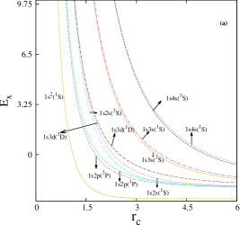
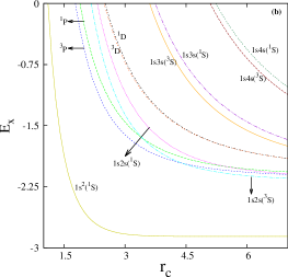
Figure 1: Energy changes in some low-lying states of confined He with $r_{c}$ in (a). Panel (b) shows a magnification of (a) in $E\leq 0$ region. See text for details.

In order to augment the discussion on excited states, Table 3 next offers specimen triplet and singlet energies of confined He corresponding to states having total orbital angular momentum $L=1,2$ arising from singly excited configurations 1s2p and 1s3d. Maintaining consistency with earlier presentation strategy, X-only results are tabulated in 2nd and 7th columns in upper (1s2p) and lower (1s3d) sections, at representative $r_{c}$’s. As before, energies monotonically fall off as the box is enlarged. Literature results in these cases are visibly scarce. For $r_{c}\geq 0.5$, STO-based RHF Yakar et al. (2011) shows, in general, nice agreement with X-only values for entire range, excepting some stray cases where, as in previous table, some spike is observed. Thus, while ³P remains within 0.02-2.02%, ¹P is estimated within 0.02-4.17%, excepting the special case for $r_{c}=2$, where an unusually large difference of 35.73% is recorded. For ^3,1P, near-HF energies within a POEP method has been reported lately Sarsa et al. (2018), for $r_{c}\geq 1$. It is encouraging to note that, for ³P, our energies match excellently with theirs, uniformly for all radii. However, for ¹P, current energies remain slightly higher when $r_{c}<5$, but steadily lowers as we approach the free-atom unconfined limit. These reference results also fully match with Luzón et al. (2020), for all available $r_{c}$. Absolute deviation relative to Sarsa et al. (2018) lies in the range of 0.001-0.08% and 0.07-4.47% for ³P, ¹P. The correlated ³P energies are found to be lower for both functionals throughout entire strength with respect to the interpolation approach of Patil and Varshni (2004) and variational scheme Banerjee et al. (2006). But for ¹P, present energies are lower in small $r_{c}$, while producing higher values in moderate to large $r_{c}$. The energy difference between two functionals gradually diminishes as confinement occurs in larger enclosures. For D states, X-only results give absolute deviations of 0.005-1.05% and 0.01-3.1% for ³D and ¹D. No literature data can be found for correlated energies, for direct comparison. Moreover, no DFT calculations are known for any of these states in this table.

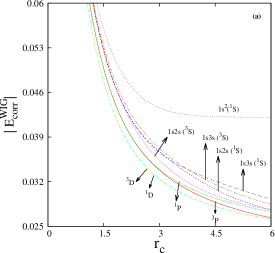
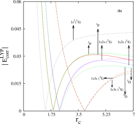
Figure 2: Absolute value of correlation energies for singly excited states of confined He, in panels (a) and (b) for Wigner and LYP functionals, with changes in box size. See text for details.

In order to illustrate the impact of confinement, energies of compressed He are portrayed in panels (a) and (b) of Fig. 1 for a few selected singlet and triplet singly excited states as a function of $r_{c}$. In addition to the states considered in above tables, here we also include 1s3s and 1s4s ^3,1S. To get a better understanding of crossing amongst various states, a magnified portion of (a) is displayed in (b) in the negative energy region, with improved resolution. Since X-only, XC-Wigner, XC-LYP energies produce qualitatively similar plots, we have taken liberty to use X-only energies to illustrate the essential features. In consonance with discussions of Tables 1-3, here also it is evident that, while influence of $v_{conf}(\mathrm{\mathbf{r}})$ seems to be more effective in smaller $r_{c}$ in low-lying states, for higher states this impact causes a shift towards larger $r_{c}$. In free He atom, the ordering of states under consideration is: E${}_{\mathrm{1s4s}(^{1}\mathrm{S})}>$ E${}_{\mathrm{1s4s}(^{3}\mathrm{S})}>$ E${}_{\mathrm{1s3d}(^{3}\mathrm{D})}>$ E${}_{\mathrm{1s3d}(^{1}\mathrm{D})}>$ E${}_{\mathrm{1s3s}(^{1}\mathrm{S})}>$ E${}_{\mathrm{1s3s}(^{3}\mathrm{S})}>$ E${}_{\mathrm{1s2p}(^{1}\mathrm{P})}>$ E${}_{\mathrm{1s2p}(^{3}\mathrm{P})}>$ E${}_{\mathrm{1s2s}(^{1}\mathrm{S})}>$ E${}_{\mathrm{1s2s}(^{3}\mathrm{S})}>$ E${}_{\mathrm{1s}^{2}(^{1}\mathrm{S})}$. With increase in confinement strength, this ordering gets dissolved due to multiple crossing between states, and rearrangement that occurs therefrom; it becomes function of $r_{c}$. Thus at $r_{c}\approx 5.3$, 4.45, 3.4, crossings occur between 1s2p ¹P, 1s2s ¹S; 1s2p ³P, 1s2s ³S; 1s2p ¹P, 1s2s ³S respectively. It is to be mentioned that, beyond the limits of $r_{c}$ presented here, several other crossings occur, which are not shown in this figure, to avoid clumsiness. This point will be further taken up in later part of this section.

Table 4: Energy difference and contribution of various components in the pair of states (1s2s ³S, 1s2p³P) and (1s3d³D, 1s2s³S) for confined He atom at different $r_{c}$’s. See text for details.

(1s2p 3P, 1s2s 3S)
	$r_{c}=0.1$	$r_{c}=0.3$	$r_{c}=0.7$	$r_{c}=1$	$r_{c}=2.5$	$r_{c}=4.4$	$r_{c}=4.5$	$r_{c}=20$
$\Delta E_{(^{3}\text{P}-^{3}\text{S})}$	$-$941.3233	$-$99.3402	$-$16.2298	$-$7.1798	$-$0.5294	$-$0.0004	0.0054	0.0437
$\Delta T_{(^{3}\text{P}-^{3}\text{S})}$	$-$964.5660	$-$107.3300	$-$19.8379	$-$9.7766	$-$1.4554	$-$0.2810	$-$0.2603	$-$0.0425
$\Delta V_{\mathrm{en}_{(^{3}\text{P}-^{3}\text{S})}}$	25.5989	8.7414	3.8949	2.7744	0.9275	0.2415	0.2265	0.0745
$\Delta V_{\mathrm{ee}_{(^{3}\text{P}-^{3}\text{S})}}$	$-$2.3561	$-$0.7517	$-$0.2868	$-$0.1776	$-$0.0015	0.0390	0.0391	0.0117
(1s3d 3D, 1s2s 3S)
	$r_{c}=0.1$	$r_{c}=0.3$	$r_{c}=0.5$	$r_{c}=1$	$r_{c}=1.1$	$r_{c}=5$	$r_{c}=10$	$r_{c}=30$
$\Delta E_{(^{3}\text{D}-^{3}\text{S})}$	$-$284.4894	$-$63.8781	$-$6.6476	$-$0.1066	0.1746	0.3722	0.1637	0.1180
$\Delta T_{(^{3}\text{D}-^{3}\text{S})}$	$-$313.2606	$-$78.4721	$-$12.7192	$-$3.2871	$-$2.7324	0.0841	$-$0.0155	$-$0.1154
$\Delta V_{\mathrm{en}_{(^{3}\text{D}-^{3}\text{S})}}$	30.0266	15.2141	6.3092	3.2885	3.0031	0.3321	0.2772	0.3948
$\Delta V_{\mathrm{ee}_{(^{3}\text{D}-^{3}\text{S})}}$	$-$1.2554	$-$0.6200	$-$0.2376	$-$0.0959	$-$0.0440	$-$0.0259	$-$0.0980	$-$0.1613

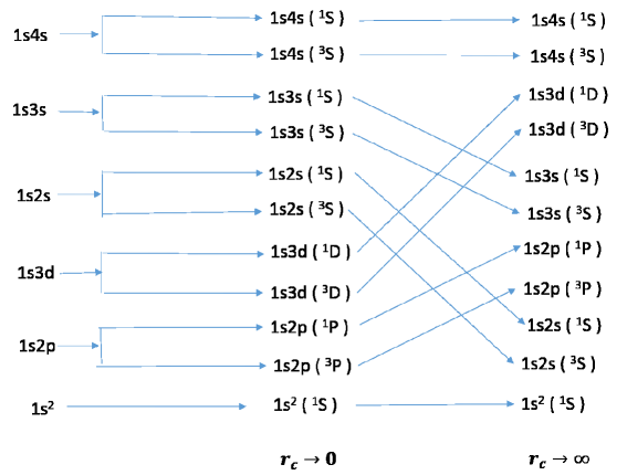
Figure 3: Correlation diagram for a He atom in an impenetrable spherical cavity of radius $r_{c}$.

From the foregoing analysis, it is obvious that energies of a confined He are less sensitive to correlation effect in stronger regime; however, with growth in $r_{c}$ the difference between X-only and correlated energies tends to assume greater significance. In Fig. 2, absolute correlation energy with respect to $r_{c}$ are plotted for some selected states. Panels (a), (b) correspond to Wigner and LYP. In both cases, it is noticed that, the nature of correlation energy with compression, maintains similar qualitative pattern for all states, for a given functional. In (a), this contribution is found to amplify steadily with confinement strength from free atom, becoming more prominent in lower $r_{c}$. Again, crossing between different states takes place quite frequently at several $r_{c}$’s. The qualitative nature of curves is comparable to the recently published results of Sarsa et al. (2016). For LYP, however, the plot in (b) considerably alters from (a); as $r_{c}$ reduces from free limit, E${}_{\mathrm{corr}}^{\mathrm{LYP}}$ lowers sharply until reaching a minimum, and then it goes up quite dramatically at certain $r_{c}$. Here also few crossovers found, which, again however, alone can not adequately explain the observed crossing pattern in energies.

The interplay between ordering and crossing of states as functions of $r_{c}$, may be analyzed by constructing a traditional correlation diagram, widely used in quantum chemistry V. I. Pupyshev and H. E. Montgomery Jr. (2017). Besides the states of previous tables, here we also include 1s3s and 1s4s ^3,1S. These are ordered according to their energies in the limit $r_{c}\rightarrow 0$ and $r_{c}\rightarrow\infty$ in middle and right segments. This diagram in Fig. 3 consists of three columns, left most of which represents two independent particles inside a small sphere. Considering this model to be a starting point, energy ordering for states of confined He within a small cavity ($r_{c}\rightarrow 0$) and free atom ($r_{c}\rightarrow\infty$) can be represented as in second and third columns. In the former case, main contribution to energy is provided by kinetic energy, while Coulombic repulsion makes a contribution that is large in absolute value, but small in comparison to kinetic energy. The energies and wave functions for a particle in a rigid sphere are available in standard text book Flügge (1971). For a system of two independent particles, energy of a state having configuration $nl,n^{\prime}l^{\prime}$, is given by a sum of orbital energies. This simplistic energy-level structure is, however, complicated in presence of an external potential due to a positive nucleus of charge $Z$ at the center of cavity. In contrast to the one-electron states of particle inside a sphere, for the atomic case, ordering of states does not necessarily remains same at all $r_{c}$ values. Due to this term in the Hamiltonian, triplet and singlet energies separate out, which is shown in mid-section $(r_{c}\rightarrow 0)$. For the limiting case $r_{c}\rightarrow\infty$, the energy levels are clearly reordered from its confined counterpart. In this scenario, our ordering matches nicely with that observed in experiment Sansonetti and Martin (2005). The transition from confinement to free case leads to interesting degeneracy points in correlation diagram as an outcome of rearrangement of states. The confinement radius for intersection point cannot be defined from the correlation diagram directly. For all states under consideration, the diagram bears qualitative resemblance to that reported in V. I. Pupyshev and H. E. Montgomery Jr. (2017) utilizing a highly accurate, correlated wave function.

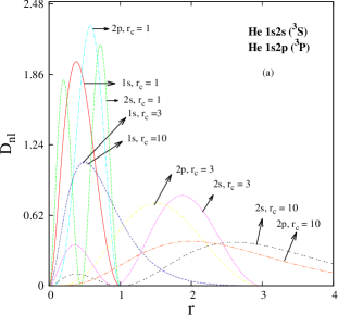
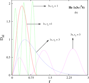
Figure 4: Radial density of orbitals of confined He, at few $r_{c}$’s in various states: (a) 1s2s ³S and 1s2p ³P (b) 1s3s ³S . See text for details.

In order to get an estimate of the above crossings among states with changes in $r_{c}$, in Table 4, as an illustration, we present total X-only energy differences, $\Delta E$, between (1s2p ³P, 1s2s ³S) and (1s3d ³D, 1s2s ³S) pair of states along with various contributions, viz., kinetic ($\Delta T$), electron-nucleus ($\Delta V_{\mathrm{en}}$) and electron-electron ($\Delta V_{\mathrm{ee}}$) at few selected $r_{c}$. Proceeding from left to right, one approaches stronger confinement to free atom. A change of sign occurs in energy difference for (³P, ³S) and (³D, ³S) in the ranges of $r_{c}=4.5$–4.4 and $r_{c}=1.1$–1.0, respectively, indicating a crossover between respective multiplet pairs. For a given state, as $r_{c}$ diminishes, so do both average electron-nucleus and electron-electron distances. This results in a lowering of $V_{\mathrm{en}}$, and increase in magnitude of $V_{\mathrm{ee}}$. Also, as a consequence of uncertainty principle, as the atom is enclosed in progressively smaller box, $T$ tends to accumulate. The relative contribution of each of these terms depends on $r_{c}$ and the particular state under consideration. The competing effects of these quantities lead to the desired crossing between various multiplets of Fig. 3; major contribution comes from one-electron energies $T$ and $V_{\mathrm{en}}$. An analysis of these components helps us conclude that for free atom as well as for some sufficiently high $r_{c}$, $\Delta V_{\mathrm{en}}$ is responsible for lower energy of ³S than ³P and ³D. For first pair, it is seen that, at $r_{c}=20$ or so, higher $T$ of ³S ($\Delta T<0$) gets compensated by comparable values of $V_{\mathrm{en}}$ and $V_{\mathrm{ee}}$ of ³P. In the second pair, for certain $r_{c}$, $V_{\mathrm{en}}$ also compensates the high $V_{\mathrm{ee}}$; thus at $r_{c}=30$, though $T$ and $V_{\mathrm{ee}}$ both are higher for ³S than ³D, $V_{\mathrm{en}}$ is responsible for (+)ve value of $\Delta E$. As we approach stronger confinement, one notices, for these pairs, $\Delta V_{\mathrm{ee}}$ hardly contributes to $\Delta E$ relative to $\Delta T$ and $\Delta V_{\mathrm{en}}$. A competition between $\Delta T$ and $\Delta V_{\mathrm{en}}$ determines the ordering between terms; $V_{\mathrm{en}}$ is higher for ³S than both ³P, ³D, but a rapid increase of $T$ for ³S compared to other states, leads to the crossing of levels. Another point to be noted is that the data presented in this table is consistent with the correlation diagram of Fig. 3; in free limit, $\Delta E$ between 1s2p ³P, 1s2s ³S is lower than the same between 1s3d ³D, 1s2s ³S, but due to crossover this pattern changes, and in the opposite limit (e.g., $r_{c}=0.1$), $\Delta E$ of former pair exceeds that of latter.

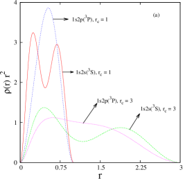
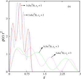
Figure 5: Radial density of (a) 1s2s ³S and 1s2p ³P (b) 1s3s ³S and 1s4s ³S states of confined He at $r_{c}=1$ and 3 respectively. Consult text for more details.

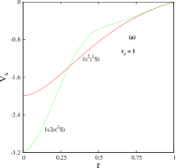
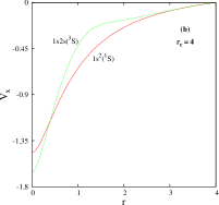
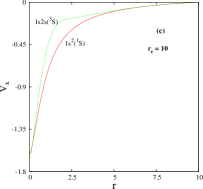
Figure 6: Exchange potential in first singlet and triplet states of confined He at $r_{c}=1,4,10$. in panels (a), (b), (c) respectively. See text for details.

Next, in Fig. 4, we plot the radial probability distribution $D_{nl}=r^{2}R_{nl}^{2}(r)$, for 1s, 2s, 2p orbitals associated with 1s2s ³S and 1s2p ³P states in panel (a), at $r_{c}$ 1, 3, 10. Similarly (b) gives for 1s, 3s orbitals related to 1s3s ³S, at $r_{c}$ 1 and 3. As expected, confinement effects are rather pronounced for outermost orbitals in comparison to other orbitals. Thus one notices that 2s, 2p, 3s densities modify significantly as the atom is squeezed at high pressure. At high $r_{c}$ (10), area under the first peak of 2s is negligible, resulting in radial density of 2s, 2p orbitals being quite similar. As confinement strengthens, latter two orbitals begin to differ from each other. Now the area of 2s orbital assumes significance relative to its free limit, while the maximum of D_2p(r) lies in between two maxima of 2s density. For 1s orbital, at $r_{c}=3$ and 10, two curves almost overlap, and as we proceed to smaller $r_{c}$ (1), the positions of maxima remain almost unaltered while height of the peaks extend. The difference between confined and unconfined charge distributions for 2s, 2p orbitals shows distinct changes. The position of nodes and local maxima are shifted to lower $r$’s and magnitudes become considerably larger. This phenomenon is more prominent for orbitals in (b) having larger number of nodes than 2s. Thus, in passing from $r_{c}=3$ (weak) to 1 (strong), 1s orbital records a change in peak height, without much shift in its position, while for 3s, in going from $r_{c}=3$ to 1, significant variations take place in nodal positions, as well as magnitude of local maxima. Hence, it is reasonable to assume that, the crossing of energy levels as discussed earlier, may be attributed mainly to adjustment of outermost orbitals, since inner orbitals change rather slowly, as pressure goes up.

Table 5: Density moments (X-only) of 1s² (¹S), 1s2s (³S) states of confined He at various $r_{c}$’s. Numbers in the parentheses denote literature results. See text for details.

$r_{c}$	1s2 1S						1s2s 3S
	$\langle\frac{1}{r^{2}}\rangle$	$\langle\frac{1}{r}\rangle$	$\langle r\rangle$	$\langle r^{2}\rangle$	$\langle r^{3}\rangle$	$\langle r^{4}\rangle$	$\langle\frac{1}{r^{2}}\rangle$	$\langle\frac{1}{r}\rangle$	$\langle r\rangle$	$\langle r^{2}\rangle$	$\langle r^{3}\rangle$	$\langle r^{4}\rangle$
0.1	1866.493	49.550	0.099	0.005	0.0003	0.00002	2865.944	56.171	0.099	0.005	0.0004	0.00003
0.3	228.700	17.099	0.290	0.048	0.008	0.001	342.610	19.183	0.295	0.053	0.010	0.002
0.5	91.406	10.653	0.473	0.128	0.038	0.012	133.083	11.807	0.486	0.145	0.0184	0.017
0.8	42.305	7.088	0.727	0.308	0.145	0.073	58.561	7.685	0.765	0.362	0.192	0.109
1.0	30.532	5.934	0.883	0.459	0.266	0.167	40.703	6.326	0.945	0.556	0.368	0.260
			(0.883,)	(0.460,	(0.267,	(0.168,
				0.459)	0.267)	0.167)
4.0	12.081	3.393	1.829	2.271	3.523	6.484	9.510	2.645	3.024	6.494	16.232	43.767
			(1.831,)	(2.272,)	(3.525,	(6.458,
					3.524)	6.456)
5.0	12.025	3.380	1.848	2.346	3.785	7.393	8.913	2.501	3.498	9.069	27.639	91.174
			(1.850,)	(2.349,) ,	(3.790,	(7.371,
					3.789)	7.366)
8.0	12.019	3.378	1.852	2.363	3.858	7.717	8.442	2.353	4.472	16.324	71.987	349.170
			(1.855,)	(2.370,	(3.880,	(7.765,
				2.369)	3.878)	7.756)
$\infty$	12.0	3.37	1.851	2.362	3.85	7.70	8.365	2.318	4.994	21.914	122.04	786.72
			(1.855,)	(2.373,	(3.891,	(7.803,
				2.372)	3.886)	7.777)

aHF result Vyboishchikov (2015).	bZMP result Vyboishchikov (2015).	cThe corresponding HF result Fischer (1977), with density normalized to unity, for
$\langle\frac{1}{r}\rangle$, $\langle r\rangle$ and $\langle r^{2}\rangle$ are 1.1544, 2.5599 and 11.5612. Present estimates are: 1.1578, 2.5030, 11.0112.

The effect of pressure on radial densities is nicely depicted in Fig. 5: panel (a) shows this for 1s2p ³P and 1s2s ³S, while (b) for 1s3s ³S and 1s4s ³S, respectively, at two representative $r_{c}$, namely, 1 and 3. One notices 4, 3, 2 and 1 maxima in 1s4s, 1s3s, 1s2s and 1s2p states. For a given state, with increasing pressure, the positions of these maxima get shifted to lower $r$, peaks become narrower and enhance in magnitude.

To pursue further, it is worthwhile to study the performance of present exchange potential. It has been compared with other accurate potentials in literature, which reproduce HF electron density. Some such examples are BJ model potential, ZMP, B88 and SC$\alpha$-LDA method. As such, $v_{x}(r)$ is calculated at each point within the work-function approximation, by solving the KS equation self-consistently for a given $r_{c}$. In Fig. 6, it is displayed at three $r_{c}$ values (1, 4, $\infty$), for ground and 1s2s (³S) states of He. Its behavior in confined environment is visibly different from that in the free limit; with lowering of $r_{c}$ it becomes steeper. For ³S state there is a distinct hump in the curve, which gets flatter with a reduction in confinement strength. An analysis of Vyboishchikov (2015) reveals that, BJ and ZMP potentials perform quite well in reproducing the exact exchange for a two-electron confined system in ground state. A comparison of our figure confirms that $v_{x}(r)$ at $r_{c}=4$ qualitatively reproduces the characteristic features found in the literature Vyboishchikov (2015).

Table 6: Ground-states energies of Li$+$ and Be²⁺ in spherical cavity of various $r_{c}$’s.

	Li+				Be2+
$r_{c}$	X-only	XC-Wigner	XC-LYP	Literature	X-only	XC-Wigner	XC-LYP	Literature
0.5	11.8249	11.7234	11.9715	11.7790,11.7768,	0.1525	0.0492	0.2767	0.1078,0.1056,
	11.82550			11.76771	0.15261			0.10801980
0.6	3.9733	3.8798	4.0774	3.9284,3.9262,	$-$6.1964	$-$6.2923	$-$6.1153	$-$6.2402,$-$6.2423,
	3.97368			3.9934290	$-$6.19641			$-$6.288159,$-$6.242352
0.7	$-$0.3149	$-$0.4019	$-$0.2422	$-$0.3590,$-$0.3611	$-$9.4540	$-$9.5441	$-$9.4046	$-$9.4970,$-$9.4991,
	$-$0.31480			$-$0.361136	$-$9.45401			$-$9.499124
0.8	$-$2.8178	$-$2.8996	$-$2.7692	$-$2.8612,$-$2.8632,	$-$11.2234	$-$11.3091	$-$11.1979	$-$11.2658,$-$11.2679,
				$-$2.893898,$-$2.863228				$-$11.26839,$-$11.267912
0.9	$-$4.3490	$-$4.4265	$-$4.3192	$-$4.3918,$-$4.3937,	$-$12.2204	$-$12.3027	$-$12.2131	$-$12.2624,$-$11.2645
	$-$4.34907			$-$4.393732	$-$12.22028
1.0	$-$5.3183	$-$5.3922	$-$5.3033	$-$5.3605,$-$5.3635,	$-$12.7954	$-$12.8750	$-$12.8021	$-$12.8369, $-$12.8393,
	$-$5.31832			$-$5.3624,$-$5.362399,	$-$12.79481			$-$12.839307
	$-$5.318324
1.2	$-$6.3632	$-$6.4318	$-$6.3698	$-$6.4047, $-$6.4065,	$-$13.3295	$-$13.4057	$-$13.3550	$-$13.3701, $-$13.3733,
	$-$6.36317			$-$6.407358	$-$13.32825			$-$13.36396
1.4	$-$6.8302	$-$6.8953	$-$6.8509	$-$6.8713, $-$6.8732,	$-$13.5151	$-$13.5894	$-$13.5515	$-$13.5552, $-$13.5590,
	$-$6.82981			$-$6.855290	$-$13.51486			$-$13.556580
1.6	$-$7.0462	$-$7.1090	$-$7.0761	$-$7.0869,$-$7.0892	$-$13.5791	$-$13.6526	$-$13.6215	$-$13.6193,$-$13.6232
	$-$7.04585				$-$13.57911
1.8	$-$7.1475	$-$7.2089	$-$7.1834	$-$7.1880, $-$7.1906,	$-$13.6007	$-$13.6738	$-$13.6465	$-$13.6415, $-$13.6449,
	$-$7.14643			$-$7.192726	$-$13.60028			$-$13.639290
2.0	$-$7.1952	$-$7.2556	$-$7.2348	$-$7.2356,,$-$7.2383,	$-$13.6079	$-$13.6808	$-$13.6555	$-$13.6493,$-$13.6521
	$-$7.19460			$-$7.238402	$-$13.61002
2.5	$-$7.2306	$-$7.2901	$-$7.2750	$-$7.2740,$-$7.258839	$-$13.6110	$-$13.6838	$-$13.6611	$-$13.6553,$-$13.654130
3.5	$-$7.2362	$-$7.2955	$-$7.2836	$-$7.2791,$-$7.279050	$-$13.6112	$-$13.6840	$-$13.6633	$-$13.6555,$-$13.655678
5.0	$-$7.2363	$-$7.2956	$-$7.2852	$-$7.2784,$-$7.2783,	$-$13.6112	$-$13.6840	$-$13.6644	$-$13.6539, $-$13.6555,
	$-$7.236415			$-$7.2798,$-$7.279254,				$-$13.657630,$-$13.655566
				$-$7.279913,
7.0	$-$7.2363	$-$7.2956	$-$7.2860	$-$7.2784,$-$7.279913	$-$13.6112	$-$13.6840	$-$13.6651	$-$13.6539,$-$13.655566
$\infty$	$-$7.2363	$-$7.2956	$-$7.2876	$-$7.2799,,$-$7.279913,	$-$13.6112	$-$13.6840	$-$13.6665	$-$13.6555,$-$13.655566
	$-$7.236415

aRef. Yakar et al. (2011).

bRef. E. V. Ludeña and M. Gregori (1979).

cRef. Flores-Riveros and Rodríguez-Contreras (2008).

dRef. Doma and El-Gammal (2012)

eRef. Bhattacharyya et al. (2013).

fRef. C. L. Wilson, H. E. Montgomery Jr., K. D. Sen, and D. C. Thompson (2010).

gRef. Joslin and Goldman (1992).

Simply looking at $\rho(r)$ plots does not provide a complete picture, as possible deviation between different densities can be sometimes very small compared with modulations in a given density at various $r$. For this, one resorts to some of the indicators (in the form of density moments) which quantitatively characterize the density distribution in a compact manner, and offer valuable insights. To this end, six expectation values, $\langle\frac{1}{r^{2}}\rangle$, $\langle\frac{1}{r}\rangle$, $\langle r\rangle$, $\langle r^{2}\rangle$, $\langle r^{3}\rangle$, $\langle r^{4}\rangle$ are offered for ground (left) and 1s2s ³S (right) states of boxed-in He, at nine selected $r_{c}$’s within the X-only framework. Only some scattered results are available for $\langle r\rangle$, $\langle r^{2}\rangle$, $\langle r^{3}\rangle$, $\langle r^{4}\rangle$ in ground state, where the obtained moments match excellently with those of ZMP and HF values Vyboishchikov (2015); in some occasions, they are completely identical. In free atom ground state, numerical HF results Fischer (1977) for $\langle\frac{1}{r}\rangle$, $\langle r\rangle$, $\langle r^{2}\rangle$ compare very nicely with current work. For excited state, no published results could be found, to the best of our knowledge. Hence, the proposed approach offers accurate moments in both confined and free atom.

III.2 Confined He-isoelectronic series

Now, we aim to analyze the role played by nuclear charge, $Z$ on the properties of atom under varying confinement strengths. In this regard, in Table 6, ground-state energies, without and with effects of correlation, are recorded for two members of He iso-electronic series (Li⁺, Be²⁺) at representative $r_{c}$, along with reference theoretical results, wherever feasible. As expected, for all systems, stronger confinement leads to enhanced total energies. The X-only results of columns 2 and 6 are compared with HF calculation Yakar et al. (2011) throughout the entire $r_{c}$; also for $Z=3$, at $r_{c}=1,5$ as well as the free atom, with that of C. L. Wilson, H. E. Montgomery Jr., K. D. Sen, and D. C. Thompson (2010). The agreement with both these references is extremely good. The correlated values of two ionic species, on the other hand, can be compared with CI E. V. Ludeña and M. Gregori (1979) and various Monte-Carlo Joslin and Goldman (1992); Doma and El-Gammal (2012) methods, in addition to Hylleraas-type Flores-Riveros and Rodríguez-Contreras (2008); C. L. Wilson, H. E. Montgomery Jr., K. D. Sen, and D. C. Thompson (2010); Bhattacharyya et al. (2013) results. The general trend is similar to that found for He. At larger $r_{c}$, difference between Wigner and LYP remains rather quite small, where both slightly underestimate literature energies. In stronger confinement region, Wigner energies appears to have a marginal edge over LYP. Taking the variational Monte-Carlo Doma and El-Gammal (2012) as reference, discrepancies appear to be slightly higher in larger $r_{c}$. As $Z$ goes up, electron density becomes more contracted; this can be looked as a shrinkage of atomic dimensions due to presence of a (+)ve charge at nucleus, which is akin to the compression of atom. However, the difference between this process and the one created by putting it inside an impenetrable cavity of varying radius is that, by enhancing $Z$, the pressure is induced centrally, whereas in latter case it is exerted peripherally. This difference is observed in energy pattern as well; the induced pressure due to growing $Z$ eventually lowers the total energy at a fixed confinement strength.

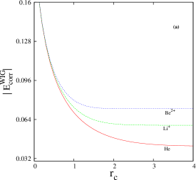
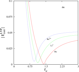
Figure 7: Absolute correlation energy, with Wigner (a) and LYP (b) functionals, in the lowest states of He, Li⁺ and Be²⁺. See text for details.

Table 7: Ground-state energies of Li and Be, confined at the center of an impenetrable spherical cavity of radius $r_{c}$. See text for details.

	Li					Be
$r_{c}$	$X-$only	Literature	XC-Wigner	XC-LYP	Literature	X-only	Literature	XC-Wigner	XC-LYP
0.5	78.4392		78.2803	78.7693		124.2082		123.9863	124.6458
0.6	48.4997		48.3534	48.7539		75.1709		74.9657	75.5088
0.7	31.1262		30.9903	31.3236		46.8218		46.6305	47.0847
0.8	20.2839		20.1567	20.4372		29.1990		29.0193	29.4035
1.0	8.2385	$-$8.5139	8.1249	8.3285		9.7334	9.7327,	9.5720	9.8537
							9.8351
1.2	2.2191	2.2191	2.1155	2.2663		0.0917	0.1368	$-$0.0560	0.1550
1.5	$-$2.2278	$-$2.2281,	$-$2.3208	$-$2.2221	$-$1.9085,	$-$6.9464	$-$6.9477,	$-$7.0796	$-$6.9391
					$-$1.9870		$-$6.92237
2.0	$-$5.1780	$-$5.1782,	$-$5.2606	$-$5.2099	$-$5.1305,	$-$11.5064	$-$11.5079,	$-$11.6244	$-$11.5503
		$-$5.1780,			$-$5.1251		$-$11.4895
		$-$5.0841					$-$11.5078
2.5	$-$6.2951	$-$6.2955	$-$6.3721	$-$6.3451		$-$13.1567	$-$13.1583,	$-$13.2660	$-$13.2261
							$-$13.1583,
							$-$13.1413
3.0	$-$6.8018	$-$6.8027	$-$6.8753	$-$6.8609	$-$6.8304,	$-$13.8614	$-$13.8613,	$-$13.9651	$-$13.9441
		$-$6.7463,			$-$6.8297		$-$13.8631,
		$-$6.8026					$-$13.8468
4.0	$-$7.2035	$-$7.2046,	$-$7.2731	$-$7.2694	$-$7.2448,	$-$14.3670	$-$14.3685,	$-$14.4645	$-$14.4606
		$-$7.1859,			$-$7.2442		$-$14.3678,
							$-$14.3521
5.0	$-$7.3383	$-$7.3395,	$-$7.4060	$-$7.4058	$-$7.3815,	$-$14.5080	$-$14.5091,	$-$14.6024	$-$14.6046
		$-$7.3230,			$-$7.3815		$-$14.4918
		$-$7.2045
6.0	$-$7.3913	$-$7.3925	$-$7.4577	$-$7.4588	$-$7.4342,	$-$14.5515	$-$14.5522,	$-$14.6443	$-$14.6488
		$-$7.3769			$-$7.4343		$-$14.5345
8.0	$-$7.4238	$-$7.4249,	$-$7.4890	$-$7.4903	$-$7.4658,	$-$14.5695	$-$14.5535,	$-$14.6612	$-$14.6672
		$-$7.4098,			$-$7.4657		$-$14.5704
		$-$7.4246
10.0	$-$7.4301	$-$7.4717,	$-$7.4948	$-$7.4962		$-$14.5711	$-$14.5729,	$-$14.6626	$-$14.6692
		$-$7.4165					$-$14.5567

aRef. Sañu-Ginartea et al. (2019)

bRef. E. V. Ludeña (1978)

cRef. A. Sarsa and C. Le Sech (2011)

dRef. Sarsa et al. (2014)

eRef. Sañu-Ginartea et al. (2018)

fRef. Rodriguez-Bautista et al. (2015)

gRef. C. Le Sech and A. Banerjee (2011)

A few words may now be devoted to the influence of $Z$ on correlation energy as confinement takes place. Thus Fig. 7 depicts how $|$E${}_{\mathrm{corr}}|$, approximated by Wigner and LYP functional, behaves with variation of $r_{c}$, in case of ground states of He, Li⁺ and Be²⁺, in panels (a) and (b). Starting from the limiting case of free ion, E${}_{\mathrm{corr}}^{\mathrm{WIG}}$, for a given member of iso-electronic series, remains practically unaffected until about $r_{c}\approx 2$ a.u.; any further compression is accompanied by a sharp increase. As $Z$ passes from 2 to 4, with lowering in $r_{c}$, the differences in $E_{\mathrm{corr}}^{\mathrm{WIG}}$ between two successive members reduce. As in stronger confinement regime, both nucleus-electron and electron-electron distances fall down; hence the effect of $Z$ gets dominated by the confining potential. This results in the fact that as $r_{c}$ declines, the plots very nearly overlap with each other. These observations reinforce the inferences drawn in our recent report Majumdar and Roy (2020). In contrast, however, panel (b) shows a distinct minimum in E${}_{\mathrm{corr}}^{\mathrm{LYP}}$ vs $r_{c}$ graph for all the species. As the cavity gets smaller, its magnitude at first diminishes steadily, then passes through a minimum and ultimately rises abruptly. This minimum is deeper and wider for He than Li⁺, which in turn, has greater measure than Be²⁺. The position of this minimum moves to lower $r_{c}$, as $Z$ advances.

III.3 Confined Li and Be atoms

Finally, we use our method to study more than two-electron systems; as sample cases we present the results for Li and Be atoms confined in an impenetrable sphere. The results for this confined three- and four-electron systems respectively, are reported for both X-only and correlated cases separately in Table 7 for ground state. For sake of comparison, along with our X-only results of Li in column 2, we provide the results from HF E. V. Ludeña (1978), direct variational Sañu-Ginartea et al. (2019) and POEP methods Sarsa et al. (2014) in column 3. As it is visible from the table, reference results are more prevalent in the region $r_{c}\geq 1$ than $r_{c}\leq 1$. The presented data for our X-only calculation are in excellent agreement with those of E. V. Ludeña (1978). Comparison with Sañu-Ginartea et al. (2019) and Sarsa et al. (2014) also show good matching. The correlated energies can be compared with variational Monte Carlo method A. Sarsa and C. Le Sech (2011) and Rayleigh-Ritz variational approach C. Le Sech and A. Banerjee (2011). For both functionals, with decreasing value of $r_{c}$ the difference between present and reference energy tends to accumulate. Furthermore, at smaller $r_{c}$ region, Wigner and LYP differ from each other significantly. Results reported for X-only energy values for Be atom are also in very good harmony with HF results of E. V. Ludeña (1978); Rodriguez-Bautista et al. (2015). No correlated results could be found in literature for confined Be. Also all the mentioned references are of wave function based method; no DFT calculation of these systems are found.

IV Concluding Remarks

A simple general and accurate KS DFT method has been proposed for calculation of an atom enclosed inside a rigid spherical cavity of varying radius. The prescription is computationally feasible and can be easily extended to other atoms/states. Properties such as energy, radial density, expectation values are reported for ground and singly excited states (1s2s ^3,1S, 1s2p ^3,1P, 1s3d ^3,1D) of He, as well as ground states of Li⁺, Be²⁺, in weak, intermediate, strong confinement strengths. Moreover, ground state results are also reported for Li and Be atoms. The overall agreement with existing literature data is excellent for the entire region, with X-only results being very close to HF. An analysis of energy ordering is offered in terms of traditional correlation diagram, and individual energy components.

To the best of our knowledge, this is the first reporting of excited state of confined atoms in very strong confinement ($r_{c}\leq 0.5$) region, excepting the work of Aquino et al. (2006), which published results for ground and singly excited (1s2s ³S, up to $r_{c}=2$) states of He. The correlation contribution to energy in smaller box ($r_{c}\leq 1$) is rather less dramatic than in a free atom. Thus, it is possible to obtain quite accurate results for a given state, provided the exchange contribution is properly accounted for, which, of course, lies behind the general success of this approach. The two correlation functionals (Wigner and LYP) behave quite differently as box size is changed. In the former, its magnitude gradually increases with confinement strength, whereas LYP shows a reduction until the appearance of a minimum at a certain $r_{c}$, followed by a steep rise. In free limit, LYP appears to perform better than Wigner. In the opposite limit, however, Wigner seems to have an edge over LYP, reflecting a trend which is qualitatively similar to that observed in literature. Confinement induces interesting energy level crossings, in conformity with Hund’s rule. When pressure enhances, the asymptotic behavior of states are greatly affected; energy level goes from an atomic mean field theory ($r_{c}\rightarrow\infty$) to particle in a hard-sphere model ($r_{c}\rightarrow 0$). These crossings are mainly attributed to X-only energy. For more accurate results, better correlation energy functionals need to be designed and employed; one such functional reported in Vyboishchikov (2017) is currently being pursued by us. Further application of the method is being made to other atoms as well as more realistic confinement scenario (such as soft or penetrable potentials). The results on these works are as encouraging as reported here. However to limit the size of this article, it appears prudent to communicate them separately in future. It would also be worthwhile to further probe the critical radii ($r_{c}$ where energies become zero), influence of electric and magnetic field through dynamical study, information theoretical analysis, etc.

V Acknowledgement

SM is grateful to IISER Kolkata for a Senior Research Fellowship. AKR gratefully acknowledges BRNS, Mumbai, India (sanction order: 58/14/03/2019-BRNS/10255) for financial support. We thank Dr. Neetik Mukherjee for giving a critical reading of the manuscript.

References

- W. Jaskólski (1996) W. Jaskólski, Phys. Rep. 271, 1 (1996).
- J. Sabin, E. Brändas, and S. Cruz (2009) (Eds.) J. Sabin, E. Brändas, and S. Cruz (Eds.), Adv. Quant. Chem., vol. 57 & 58 (Academic Press, New York, 2009).
- K. D. Sen (2014) (Ed.) K. D. Sen (Ed.), Electronic Structure of Quantum Confined Atoms and Molecules (Springer International Publishing, Switzerland, 2014).
- E. Ley-Koo (2018) E. Ley-Koo, Revista Mexicana de Física 64, 326 (2018).
- Michels et al. (1937) A. Michels, J. de Boer, and A. Bijl, Physica 4, 981 (1937).
- Burrows and Cohen (2006) B. L. Burrows and M. Cohen, Int. J. Quant. Chem. 106, 478 (2006).
- C. A. Ten Seldam and S. R. De Groot (1952) C. A. Ten Seldam and S. R. De Groot, Physica 18, 891 (1952).
- E. V. Ludeña (1978) E. V. Ludeña, J. Chem. Phys. 69, 1770 (1978).
- E. V. Ludeña and M. Gregori (1979) E. V. Ludeña and M. Gregori, J. Chem. Phys. 71, 2235 (1979).
- Rivelino and Vianna (2001) R. Rivelino and J. D. M. Vianna, J. Phys. B 34, L645 (2001).
- Joslin and Goldman (1992) C. Joslin and S. Goldman, J. Phys. B 25, 1965 (1992).
- Marín and Cruz (1991) J. L. Marín and S. A. Cruz, J. Phys. B 24, 2899 (1991).
- Banerjee et al. (2006) A. Banerjee, C. Kamal, and A. Chowdhury, Phys. Lett. A 350, 121 (2006).
- A. Flores-Riveros, N. Aquino, and H. E. Montgomery Jr. (2010) A. Flores-Riveros, N. Aquino, and H. E. Montgomery Jr., Phys. Lett. A. 374, 1246 (2010).
- C. Le Sech and A. Banerjee (2011) C. Le Sech and A. Banerjee, J. Phys. B 44, 105003 (2011).
- Ting-yun et al. (2001) S. Ting-yun, B. Cheng-Guang, and L. Bai-Wen, Commun. Theor. Phys. 35, 195 (2001).
- H. E. Montgomery Jr., N. Aquino, and A. Flores-Riveros (2010) H. E. Montgomery Jr., N. Aquino, and A. Flores-Riveros, Phys. Lett. A 374, 2044 (2010).
- Aquino et al. (2003) N. Aquino, A. Flores-Riveros, and J. F. Rivas-Silva, Phys. Lett. A 307, 326 (2003).
- Flores-Riveros and Rodríguez-Contreras (2008) A. Flores-Riveros and A. Rodríguez-Contreras, Phys. Lett. A. 372, 6175 (2008).
- C. Laughlin and S. I. Chu (2009) C. Laughlin and S. I. Chu, J. Phys. A 42, 265004 (2009).
- C. L. Wilson, H. E. Montgomery Jr., K. D. Sen, and D. C. Thompson (2010) C. L. Wilson, H. E. Montgomery Jr., K. D. Sen, and D. C. Thompson, Phys. Lett. A. 374, 4415 (2010).
- H. E. Montgomery Jr. and V. I. Pupyshev (2013) H. E. Montgomery Jr. and V. I. Pupyshev, Phys. Lett. A 377, 2880 (2013).
- Bhattacharyya et al. (2013) S. Bhattacharyya, J. K. Saha, P. K. Mukherjee, and T. K. Mukherjee, Phys. Scr. 87, 065305 (2013).
- H. E. Montgomery Jr. and V. I. Pupyshev (2015) H. E. Montgomery Jr. and V. I. Pupyshev, Theor. Chem. Acc. 134, 1598 (2015).
- Saha et al. (2016) J. Saha, S. Bhattacharyya, and T. K. Mukherjee, Int. J. Quantum Chem. 116, 1802 (2016).
- Yakar et al. (2011) Y. Yakar, B. Çakir, and A. Özmen, Int. J. Quantum Chem. 111, 4139 (2011).
- Doma and El-Gammal (2012) S. B. Doma and F. N. El-Gammal, J. Theor. Appl. Phys. 6, 28 (2012).
- A. Sarsa and C. Le Sech (2011) A. Sarsa and C. Le Sech, J. Chem. Theory Comput. 7, 2786 (2011).
- Young et al. (2016) T. D. Young, R. Vargas, and J. Garza, Phys. Lett. A. 380, 712 (2016).
- V. I. Pupyshev and H. E. Montgomery Jr. (2017) V. I. Pupyshev and H. E. Montgomery Jr., Theor. Chem. Acc. 136, 138 (2017).
- Garza et al. (2012) J. Garza, J. M. Hernández-Pérez, J.-Z. Ramírez, and R. Vargas, J. Phys. B 45, 015002 (2012).
- Connerade et al. (2000) J. P. Connerade, V. K. Dolmatov, and P. A. Lakshmi, J. Phys. B 33, 251 (2000).
- Patil et al. (2005) S. H. Patil, K. D. Sen, and Y. P. Varshni, Can. J. Phys. 83, 919 (2005).
- Sarsa et al. (2014) A. Sarsa, E. Buendía, and F. J. Gálvez, J. Phys. B. 47, 185002 (2014).
- Ludlow and Lee (2015) J. A. Ludlow and T. G. Lee, Phys. Rev. A 91, 032507 (2015).
- Gálvez et al. (2017) F. J. Gálvez, E. Buendía, and A. Sarsa, Int. J. Quantum Chem. 117, e25421 (2017).
- Martínez-Sánchez et al. (2016) M.-A. Martínez-Sánchez, M. Rodriguez-Bautista, R. Vargas, and J. Garza, Theor. Chem. Acc. 135, 207 (2016).
- Vyboishchikov (2016) S. F. Vyboishchikov, J. Comput. Chem. 37, 2677 (2016).
- Buchachenko (2001) A. L. Buchachenko, J. Phys. Chem. B 105, 5839 (2001).
- Dolmatov et al. (2004) V. K. Dolmatov, A. S. Baltenkov, J.-P. Connerade, and S. T. Manson, Radiat. Phys. Chem. 70, 417 (2004).
- Grochala et al. (2007) W. Grochala, R. Hoffmann, J. Feng, and N. Ashcroft, Angew. Chem. Int. Ed. 36, 3620 (2007).
- Parr and Yang (1989) R. G. Parr and W. Yang, Density Functional Theory of Atoms and Molecules (Oxford University Press, New York, 1989).
- Becke (1988) A. D. Becke, Phys. Rev. A 38, 3098 (1988).
- Garza et al. (1998) J. Garza, R. Vargas, and A. Vela, Phys. Rev. E 58, 3949 (1998).
- Aquino et al. (2006) N. Aquino, A. Flores-Riveros, J. F. Rivas-Silva, and K. D. Sen, J. Chem. Phys. 124, 054311 (2006).
- Perdew and Wang (1992) J. P. Perdew and Y. Wang, Phys. Rev. B 45, 13244 (1992).
- Garza et al. (2005) J. Garza, R. Vargas, N. Aquino, and K. D. Sen, J. Chem. Sci. 117, 379 (2005).
- Borgoo et al. (2008) A. Borgoo, D. J. Tozer, P. Geerlings, and F. D. Proft, Phys. Chem. Chem. Phys. 10, 1406 (2008).
- Waugh et al. (2010) S. Waugh, A. Chowdhury, and A. Banerjee, J. Phys. B 43, 225002 (2010).
- Vyboishchikov (2015) S. F. Vyboishchikov, J. Comput. Chem. 36, 2037 (2015).
- Vyboishchikov (2017) S. F. Vyboishchikov, Chem. Phys. Chem. 18, 3478 (2017).
- Duarte-Alcaráz et al. (2019) F.-A. Duarte-Alcaráz, M.-A. Martínez-Sánchez, M. Rivera-Almazo, R. Vargas, R. Rosas-Burgos, and J. Garza, J. Phys. B 52, 135002 (2019).
- Lozano-Espinosa et al. (2017) M. Lozano-Espinosa, J. Garza, and M. Galván, Phil. Mag. 97, 284 (2017).
- Chakraborty and Chattaraj (2019) D. Chakraborty and P. K. Chattaraj, J. Phys. Chem. A 123, 4513 (2019).
- Sahni and Harbola (1990) V. Sahni and M. Harbola, Int. J. Quant. Chem. Symp. 24, 569 (1990).
- Sahni et al. (1992) V. Sahni, Y. Li, and M. Harbola, Phys. Rev. A 45, 1434 (1992).
- Brual and Rothstein (1978) G. Brual and S. M. Rothstein, J. Chem. Phys. 69, 1177 (1978).
- Lee et al. (1988) C. Lee, Y. Wang, and R. G. Parr, Phys. Rev. B 37, 785 (1988).
- Singh and Deb (1996) R. Singh and B. M. Deb, J. Chem. Phys. 104, 5892 (1996).
- Roy et al. (1997a) A. K. Roy, R. Singh, and B. M. Deb, J. Phys. B 30, 4763 (1997a).
- Roy et al. (1997b) A. K. Roy, R. Singh, and B. M. Deb, Int. J. Quant. Chem. 65, 317 (1997b).
- Roy and Chu (2002) A. K. Roy and S. I. Chu, Phys. Rev. A 65, 052508 (2002).
- Roy (2004a) A. K. Roy, J. Phys. B 37, 4369 (2004a).
- Roy (2005) A. K. Roy, J. Phys. B. 38, 1591 (2005).
- Majumdar and Roy (2020) S. Majumdar and A. K. Roy, Quant. Rep. 2, 189 (2020).
- Roy (2004b) A. K. Roy, Phys. Lett. A 321, 231 (2004b).
- Roy (2004c) A. K. Roy, J. Phys. G 30, 269 (2004c).
- Ziegler et al. (1977) T. Ziegler, A. Rauk, and E. J. Baerends, Thero. Chim. Acta 43, 261 (1977).
- Gimarc (1967) B. M. Gimarc, J. Chem. Phys. 47, 5110 (1967).
- Dirac (1930) P. A. M. Dirac, Proc. Camb. Phil. Soc. 26, 376 (1930).
- Luzón et al. (2020) A. Luzón, E. Buendía, and F. J. Gálvez, Int. J. Quantum Chem. 120, e26048 (2020).
- Sarsa et al. (2018) A. Sarsa, E. Buendía, F. J. Gálvez, and J. Katriel, Chem. Phys. Lett. 702, 106 (2018).
- Patil and Varshni (2004) S. H. Patil and Y. P. Varshni, Can. J. Phys 82, 647 (2004).
- Sarsa et al. (2016) A. Sarsa, E. Buendía, and F. J. Gálvez, J. Phys. B. 49, 145003 (2016).
- Flügge (1971) S. Flügge, Practical quantum mechanics I (Springer, Berlin, 1971).
- Sansonetti and Martin (2005) J. E. Sansonetti and W. C. Martin, J. Phys. Chem. Ref. Data 34, 1559 (2005).
- Fischer (1977) C. F. Fischer, The Hartree-Fock Method For Atoms (Wiley, New York, 1977).
- Sañu-Ginartea et al. (2019) A. D. Sañu-Ginartea, E. M. Guillén-Romeroa, L. Ferrer-Galindob, L. A. Ferrer-Moreno, R. Betancourt-Riera, and R. Riera, Results in Phys. 13, 102261 (2019).
- Sañu-Ginartea et al. (2018) A. D. Sañu-Ginartea, L. Ferrer-Galindob, R. A. Rossa, A. Corella-Madueño, R. Betancourt-Riera, L. A. Ferrer-Moreno, and R. Riera, J. Phys. Commun. 2, 015001 (2018).
- Rodriguez-Bautista et al. (2015) M. Rodriguez-Bautista, C. Díaz-García, A. M. Navarrete-López, R. Vargas, and J. Garza, J. Chem. Phys. 143, 034103 (2015).