TRT-ViT: TensorRT-oriented Vision Transformer

Abstract

We revisit the existing excellent Transformers from the perspective of practical application. Most of them are not even as efficient as the basic ResNets series and deviate from the realistic deployment scenario. It may be due to the current criterion to measure computation efficiency, such as FLOPs or parameters is one-sided, sub-optimal, and hardware-insensitive. Thus, this paper directly treats the TensorRT latency on the specific hardware as an efficiency metric, which provides more comprehensive feedback involving computational capacity, memory cost, and bandwidth. Based on a series of controlled experiments, this work derives four practical guidelines for TensorRT-oriented and deployment-friendly network design, e.g., early CNN and late Transformer at stage-level, early Transformer and late CNN at block-level. Accordingly, a family of TensortRT-oriented Transformers is presented, abbreviated as TRT-ViT. Extensive experiments demonstrate that TRT-ViT significantly outperforms existing ConvNets and vision Transformers with respect to the latency/accuracy trade-off across diverse visual tasks, e.g., image classification, object detection and semantic segmentation. For example, at 82.7% ImageNet-1k top-1 accuracy, TRT-ViT is 2.7$\times$ faster than CSWin and 2.0$\times$ faster than Twins. On the MS-COCO object detection task, TRT-ViT achieves comparable performance with Twins, while the inference speed is increased by 2.8$\times$.

1 Introduction

Recently, Vision Transformer has witnessed prevailing success and achieved noticeable performance gain over CNN in various computer vision tasks, such as image classification, semantic segmentation, and object detection, etc. However, CNN still dominates the visual architecture from the perspective of real-scene deployment. When we dig deep into substantial performance improvements behind existing Transformers, we observe that these gains come at the cost of extensive resource overhead. Moreover, it has become a demanding obstacle when the Transformer is deployed on resource-constrained devices. To alleviate unwieldy computational cost of Transformer, a series of works pay much attention to developing efficient Vision Transformer, such as Swin Transformer Swin , PVT PVT_v1 , Twins Twins , CoAtNetCoatnet and MobileViTMobileViT .

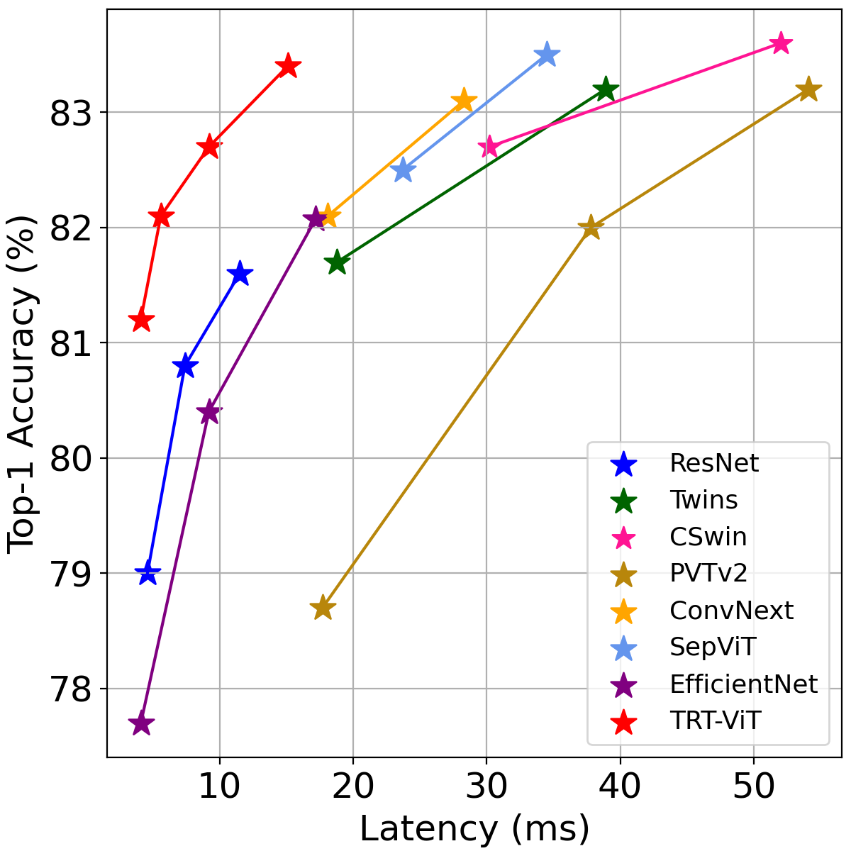
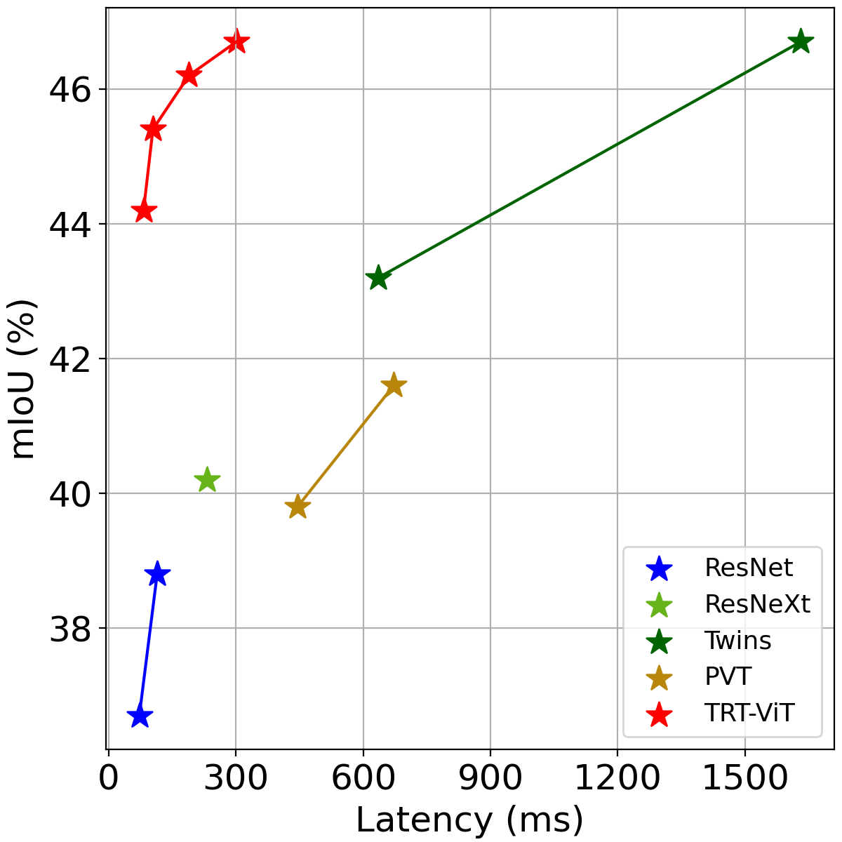
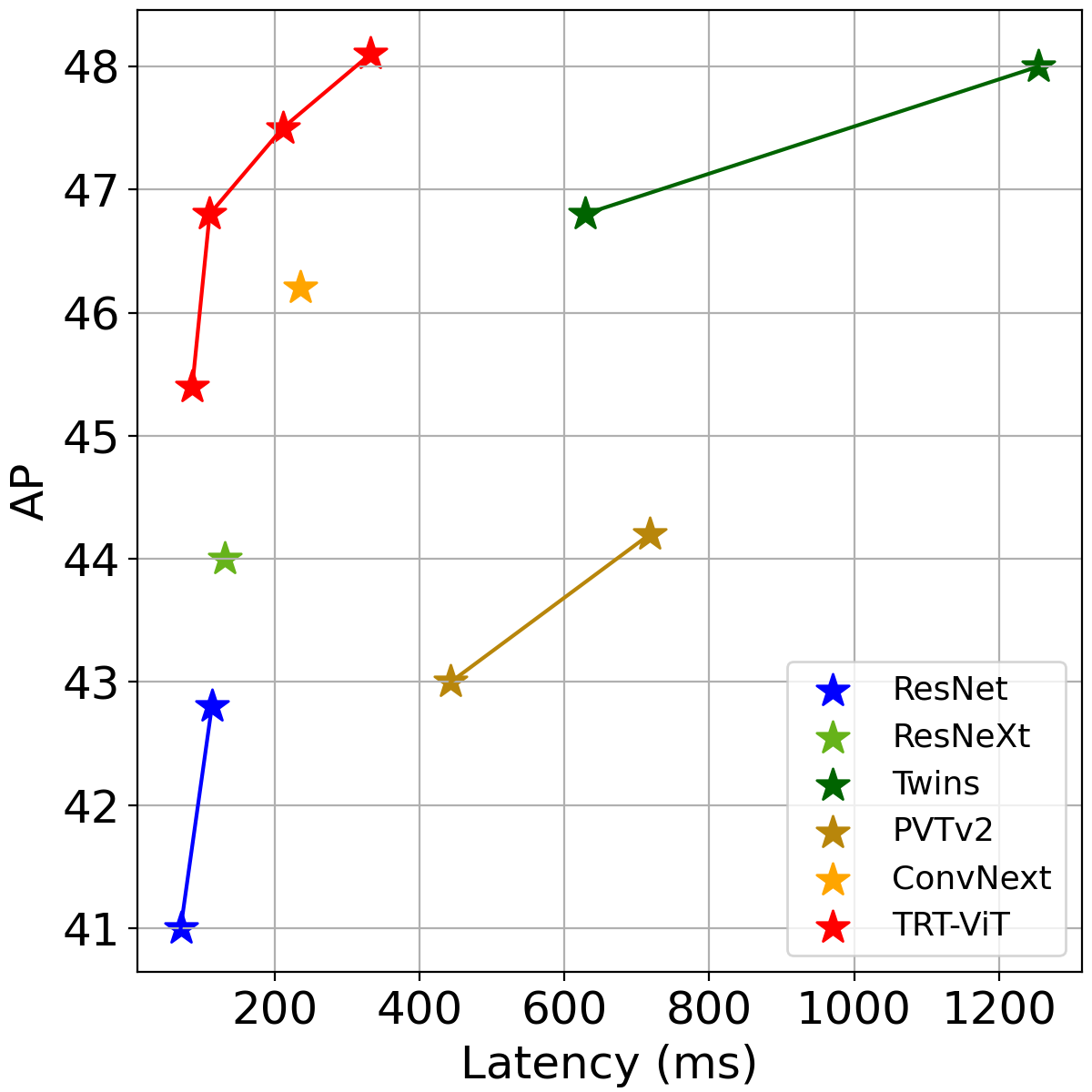
Figure 1: Comparison among TRT-ViT and efficient Networks, in terms of accuracy-latency trade-off. (a): ImageNet classification; (b): ADE20K Semantic Segmentation; (c): COCO Object Detection. TRT-ViT consistently outperforms the SOTA efficient Networks. Latency is measured on the TensorRT framework with a T4 GPU (batch size=8)

Although the above works showed the efficiency of ViTs from different points of view, the critical design is mainly guided by the indirect criterion of computation efficiencies, such as FLOPs or parameters. This circuitous criterion is one-sided, sub-optimal, and deviating from real-scene deployment. In fact, the model has to cope with environmental uncertainty in the deployment procedure, which involve hardware-aware characteristics such as memory access cost and I/O throughput. Specifically, as stated in many papers (e.g.,ShuffleNet_v2 ; GPUNet ), the indirect metric of computation complexity is widely used in neural network architecture design that FLOPs and parameters are approximations of, but usually can not truly reflect the direct metric that we really care about, such as speed or latency. In this paper, to address such discrepancy, we provide a view that treats the TensorRT latency on the specific hardware as direct efficiency feedback. TensorRT has become a general and deployment-friendly solution in practical scenarios, and it helps to provide convincing hardware-oriented guidance. With this direct and accurate guidance, we redraw the accuracy and efficiency trade-off diagram of several existing competitive models in Figure 1. As depicted in Figure 1, Transformer has the advantage of good performance, while CNN successes in high efficiency. Although ResNet is not as impressive as the competitive Transformers in performance, it is still the best architecture under the accuracy-latency trade-off. For example, ResNet employs 11.7 milliseconds (batch size = 8) to achieve 81.7% accuracy. Although twins-pcpvt-s achieves an impressive accuracy, 83.4% in imagenet-1k classification, it takes up to 39.8 milliseconds to achieve this goal. These observations motivate us to raise a question: how to design a model that can perform as well as Transformer and predict as fast as ResNet?

To answer this question, we systematically explore the hybrid design of CNNs and Transformers. We follow the stage-to-block hierarchical roadmap to investigate the TensorRT-oriented architecture. Through extensive experiments, we summarize four practical guidelines to design efficient networks on TensorRT: 1) stage-level: Transformer block at the late stages maximizes the trade-off between efficiency and performance; 2) stage-level: shallow-then-deep stage pattern improves the performance; 3) block-level: a block mixed of Transformer and BottleNeck is more efficient than Transformer.; 4) block-level: global-then-local block pattern helps make up the performance issue.

Based on the above guidelines, we design a family of TensortRT-oriented Transformers (abbreviated as TRT-ViT), consisted of hybrid networks with ConvNets and Transformers. CNN and Transformer are position-complementary in stage and block-level at TRT-ViT. Furthermore, we propose various TRT-ViT blocks to combine CNN and Transformer in a serial scheme that decouples heterogeneous concepts and improves the efficiency of information flow. The proposed TRT-ViT outperforms existing ConvNets and vision Transformers with respect to the latency-accuracy trade-off on image classification. For example, at 82.7% ImageNet-1k top-1 accuracy, TRT-ViT is 2.7$\times$ faster than CSWin and 2.0$\times$ faster than Twins.

More importantly, TRT-ViT shows a more significant latency/accuracy trade-off gain on downstream tasks. As depicted in Figure  1, TRT-ViT achieves comparable performance with Twins, while the inference speed is increased by 2.8$\times$ on the MS-COCO object detection and 4.4$\times$ on ADE20K semantic segmentation task. TRT-ViT outperforms ResNet by 3.2 AP (from 40.4 to 43.6) on COCO detection and 6.6% (from 38.86% to 45.46%) on ADE20K segmentation under similar TensorRT latency.

We believe that our work points out a viable path for scientific research towards industrial deployment in terms of architecture design, which significantly reduces the gap between laboratory research and real-scene practice. We hope that our work can provide inspiring insight and encourage more researchers to be involved in real-scene architecture design.

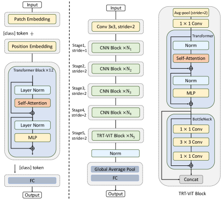
Figure 2: The overall framework TRT-ViT. Left: ViT model. Right: Our proposed TRT-ViT model.

2 Related Work

Convolutional networks. Convolutional neural networks (CNNs) have dominated the visual architecture in various computer vision tasks in the past decade, including image classification, object detection, semantic segmentation. ResNetResNet employs residual connections to relieve the network degradation, ensuring the network builds deeper to capture high-level abstraction. DenseNetDenseNet alternatively enhances feature reuse and connects the feature maps via dense connections. MobileNetsMobilenets ; MobileNet_v2 introduces depthwise convolutions and pointwise convolutions to enhance model efficiency. ShuffleNetShufflenet ; ShuffleNet_v2 adopts group convolution and channel shuffle to reduce the computational cost further. ConvNextConvNext reviews the design of the vision Transformers and reveals that the CNN-only architecture also can achieve comparable results with Transformers.

Vision Transformers. Transformers are first proposed in the field of natural language processing. Vision Transformer(ViT)ViT shows that Transformer can also achieve impressive performance on multiple vision tasks. ViT splits the image into patches and treats the patches as words to perform self-attention. DeiTDeit proposes the hierarchical Transformers to handle high-resolution images. T2T-ViTT2T gradually converts the image into a token by recursively aggregating adjacent tokens. Swin TransformerSwin computes attention within the shifted window. PiTPiT jointly uses pooling layer and depthwise convolution layer to achieve channel multiplication and spatial reduction. Nowadays, researchers pay more attention to efficiency, including efficient self-attention, training strategies, pyramidal designs, etc.

Hybrid Models. Recent works show that combining convolution and Transformer as a hybrid architecture helps absorb the advantages of both architectures. BoTNetBoTNet replaces the last three blocks of ResNet with a self-attention block, and CvTCvT introduces depthwise and pointwise convolution in front of self-attention. The CMTCmt block consists of depthwise convolution based local perception unit and a light-weight transformer module. LeViTLeViT substitutes the patchy stem with a convolutional stem to reduce computation cost. In MobileViTMobileViT , MobileNetV2 block and Transformer block are combined in series and a MobileVit block is developed to learn global representations. But MobileVit is still relatively heavy compared to Mobile CNNs. Mobile-FormerMobile-Former builds bidirectional fusion between Transformer and Mobilenets to capture local and holistic concepts. In this paper, we design a family of TensorRT-oriented hybrid models that adapt more to the actual development scenarios.

3 Approach

In this section, we first present a series of empirical findings and propose four practical guidelines for designing efficient networks on TensorRT. Then we develop a new architecture with high efficiency and performance, denoted as TRT-ViT.

3.1 Practical Guidelines for Efficient Network Design on TensorRT

Our study is performed on the widely adopted high-performance inference SDK, TensorRT. To initiate our study, we analyze the runtime performance of two SOTA networks, ResNet ResNet and ViT ViT . They are both highly accurate on the ImageNet1K classification task and prevalent in the industry. Although we only analyze these two networks, we note that they are representative of the current trend. At their core are BottleNeck block and Transformer block, which are also crucial components for other state-of-the-art networks, such as ConvNext ConvNext , and Swin Swin .

To better illustrate our empirical results, follow RepLKNetRepLKNet , we use the computational density (measured in Tera FLoating-point Operations Per Second, TeraFLOPS) of an operation or block to quantify its efficiency on a hardware, described as follows

$$\text{TeraFLOPS}=\frac{\text{FLOPs}}{\text{Latency}}$$ (1)

As seen from Figure 1(a) and Table1, BottleNeck block is more efficient and has a higher TeraFLOPS, while Transformer block is more powerful and has better accuracy on ImageNet. In this paper, we aim to design a network that achieves ResNet-like efficiency and Transformer-like performance. It is straightforward to design a network that is mixed of BottleNeck and Transformer block, e.g., MobileViTMobileViT . However, these papers either focus on optimizing FLOPs, which is an indirect criterion to measure the efficiency, or put much effort into mobile devices.

Trivially applying Transformer to CNNs usually leads to inferior performance and speed. Hence, we summarize four practical guidelines for effectively designing efficient networks on TensorRT.

Table 1: Analyze TeraFLOPS on TensorRT. Latency is measured on the TensorRT framework with a T4 GPU (batch size=16).

Block Type	Feature map size	Params(K)	FLOPs(M)	Latency(ms)	TeraParams($\uparrow$)	TeraFLOPS($\uparrow$)
Transformer	256$\times$56$\times$56	658	7098	86.9	7.5	81
	512$\times$28$\times$28	2627	2688	14.6	179	184
	1024$\times$14$\times$14	10498	2135	4.92	2142	435
	2048$\times$7$\times$7	41960	2066	3.51	11988	599
BottleNeck	256$\times$56$\times$56	70	218	0.58	120	378
	512$\times$28$\times$28	279	218	0.38	733	573
	1024$\times$14$\times$14	1114	218	0.35	3173	620
	2048$\times$7$\times$7	4456	218	0.33	13723	670
MixBlockA	256$\times$56$\times$56	216	3195	27.1	7.9	117
	512$\times$28$\times$28	860	989	4.80	182	206
	1024$\times$14$\times$14	3400	712	1.56	2200	456
	2048$\times$7$\times$7	13710	676	1.08	12694	625
MixBlockB/C	256$\times$56$\times$56	216	3195	26.1	8.1	122
	512$\times$28$\times$28	860	989	4.50	191	219
	1024$\times$14$\times$14	3400	712	1.51	2288	474
	2048$\times$7$\times$7	13710	676	1.05	13057	644

Guideline 1: Transformer block at the late stages maximizes the trade-off between efficiency and performance. It is believed that Transformer block is more powerful but less efficient than the convolution block because the Transformer aims to build a global connection between features. In contrast, convolution only captures the local information Swin ; Twins . Here, we provide a detailed analysis equipped with TensorRT. As verified from Figure 1, stacking Transformer blocks(PVT-Medium) gives $81.2\%$ Top-1 accuracy on ImageNet1K classification task while the corresponding accuracy of BottleNeck blocks(ResNet50) is only $79.0\%$. However, as shown in Table 1, when it comes to efficiency, BottleNeck block always outperforms Transformer block in terms of TeraFLOPS under various input resolutions.

Furthermore, the efficiency gap between Transformer and BottleNeck decreases when the input resolution decreases. Specifically, TeraFLOPS value of Transformer is only 81, less than quarter of the BottleNeck’s TeraFLOPS value 378, when the input resolution is $56\times 56$. However, when the resolution decreases to $7\times 7$, Transformer’s TeraFLOPS value is almost equal to BottleNeck, which is 599 and 670, respectively. This observation motivates us to put Transformer blocks at the late stages to balance performance and efficiency when designing efficient networks on TensorRT. Although some researchers(e.g., CoATNetCoatnet ) follow similar rules and propose networks mixed with Transformer and CNN blocks, to our best knowledge, we are the first to provide quantitative analysis on TensorRT.

Following guideline 1, a native solution is to replace BottleNeck blocks with Transformer blocks at the late stages, dubbed as MixNetV (MixNet Valilla) in Table 1. We can see that MixNetV is faster than ViT and more accurate than ResNet.

Guideline 2: shallow-then-deep stage pattern improves the performance. It is a widely held view that the more parameters, the higher the model capacity. We aim to develop a stage pattern that owns more parameters without sacrificing efficiency. We first define the parameter density of an operation or block to quantify its capacity on hardware, similar to TeraFLOPs in Equ. 1, as follows:

$$\text{TeraParams}=\frac{\text{Params}}{\text{Latency}}$$ (2)

We study the property of TeraParams in various SOTA networks, e.g., RestNet and ViT, and present our findings in Table 1. The TeraParams of BottleNeck are getting more prominent in the late stages, which indicates that stacking more BottleNeck blocks at the late stage will result in larger model capacity, compared to the early stage. A similar trend can also be found in Transformer block in ViT. This observation inspires us to make the early stages shallower and the late stages deeper. We assume this shallow-then-deep stage pattern will bring more parameters, improve the model capacity and result in better performance without degrading the efficiency. To verify this, we make corresponding modifications on ResNet50 and provide the empirical results in Table 2. We reduce the stage depth of the first and second stages from 3, 4 to 2, 3, respectively, while increasing the stage depth of the last stage from 3 to 5. From Table 2, we can see that Refined-ResNet50 outperforms ResNet50 by $0.3\%$ Top-1 accuracy on ImageNet1K while being slightly faster on TensorRT. Furthermore, we apply this shallow-then-deep stage pattern to PvT-Small and get Refined-PvT-Small, which is better and faster. Finally, a similar conclusion can be made on MixNetV, which comes as no surprise.

Table 2: Stage depth comparsion. Latency is measured on the TensorRT framework with a T4 GPU (batch size=8).

Model	Stage depth	FLOPs(G)	Param(M)	Latency(ms)	Top-1 Acc(%)
ResNet50ResNet	3-4-6-3	4.1	25.6	4.6	79.0
Refined-ResNet50	2-3-6-5	4.1	34.1	4.4	79.3
PVT-Small PVT_v1	3-4-6-3	3.8	24.5	20.7	79.8
Refined-PVT-Small	2-3-6-5	3.6	29.8	17.9	80.2
MixNetV	3-5-6-3	4.3	53.5	6.9	80.5
Refined-MixNetV	2-3-6-4	4.8	69.6	6.8	80.8

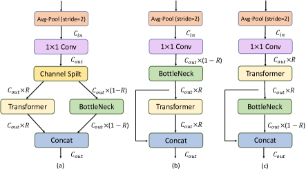
Figure 3: The proposed TRT-ViT block. (a): MixBlockA. (b): MixBlockB (c): MixBlockC. We use avgpool to downsamle while $\text{stride}=2$.

Guideline 3: a block mixed of Transformer and BottleNeck is more efficient than Transformer. Although we have achieved significant improvement following Guidelines 1 and 2, Refined-MixNetV can not dominate ResNet in efficiency. Our goal is to build a network with ResNet-like efficiency and ViT-like performance. To achieve this, we seek to design a new block mixed of Transformer and BottleNeck by leveraging the benefits of both.

We provide two mixed blocks in Figure 3(a) and (b) where a $1\times 1\text{Conv}$ layer is first utilized to project the number of input channels, and a Concat layer is used to merge the global and local feature at the end. A shrinking ratio $R$ is introduced to control the proportion of Transformer block in the mixed block, defined as the output channel of Transformer block divided by $C_{out}$, the output channel of the mixed block. As depicted in Figure3(a), in MixBlockA, two branches are created, one for Transformer and the other for BottleNeck. In addition, a channel split layer is used to improve further the efficiency, where the output channel for Transformer block is $C_{out}\times R$ while the corresponding one is $C_{out}\times(1-R)$. In MixBlockB, Transformer block and BottleNeck block are stacked sequentially and the output channel of Transformer block and BottleNeck block are equal, i.e., $R=0.5$ here. As we can see from Table 1, TeraFLOPS of both mixed blocks are significantly increased compared to Transformer block, which indicates the mixed blocks are more efficient than Transformer block. Moreover, their corresponding TeraParams are also better, which shows they have the potential to achieve better performance.

Replacing Transformer block in MixNetV with MixBlockA and MixBlockB, we build MixNetA and MixNetB. As depicted in Table 3, where C, T and M denote Convolution, Transformer and MixBlock respectively, we can see that both MixNetA and MixNetB outperform ResNet50. However, neither of them can beat MixNetV in terms of accuracy. Moreover, the performance gap between PVT-Medium and both mixed nets can not be neglected.

Table 3: Blcok type comparsion. Latency is measured on the TensorRT framework with a T4 GPU (batch size=8).

Model	Block-type	FLOPs(G)	Latency(ms)	Top-1 Acc(%)
ResNet50	C-C-C-C	4.1	4.6	79.0
PVT-Medium	T-T-T-T	6.7	30.0	81.2
MixNetV	C-C-C-T	4.8	6.8	80.8
MixNetA	C-C-C-M	2.7	4.3	80.7
MixNetB	C-C-C-M	2.7	4.1	80.3
MixNetC	C-C-C-M	2.7	4.1	81.2

Guideline 4: global-then-local block pattern helps to make up the performance issue. As described in many papers Swin ; PVT_v1 ; Twins , Transformer whose receptive field is usually huge extracts global information from input features and enables information exchange within each entry. In contrast, Convolution, whose small receptive field only mines local information. It makes more sense to acquire global information first and refine it locally instead of extracting local information first and refining it globally. Moreover, the shrinking ratio $R$ in MixBlockB has to be 0.5, losing the flexibility to make a further adjustment. The global-then-local block pattern solves this issue, where $R$ can be any value between 0 and 1.

Following this rule, we switch the order of Transformer operation and Convolution operation in MixBlockB and get MixBlockC, as depicted in Figure 3(c). The TeraFLOPS score of MixBlockC is equivalent to MixBlockB. Then, substituting MixBlockB with MixBlockC, we get MixNetC. In coincidence with our intuition, as shown in Table 3, MixNetC performs better than MixNetB without any sacrifice of efficiency. Moreover, MixNetC surpasses MixNetV in terms of both accuracy and TRT latency. Besides, the gap between MixNetC and PVT-Medium is bridged and MixNetC achieves ResNet-like efficiency and Transformer-like performance.

We use MixBlockC as the basic building block in the rest of the paper.

3.2 TRT-ViT: An Efficient Network on TensorRT

We build our TRT-ViT architecture following the basic configuration of ResNet ResNet , where feature pyramid structure is adopted and the resolution of feature maps decreases with network depth while the number of channels increases. Next, we apply our proposed practical guidelines to construct TRT-ViT. The whole architecture is divided into five stages, and we only use MixBlockC in the late stages, while convolution layers are used in the early stages. Besides, we utilize a shallow-then-deep stage pattern, where early stages are shallower and late stages are deeper, compared to the stage pattern in ResNet.

To provide a fair comparison with other SOTA networks, we propose four variants, TRT-ViT-A/B/C/D, whose configurations are listed in Table4. $3\times 3$ denotes convolution with kernel size =3 and C represents the output channel of a stage. $R,S,K$ are inter parameters in the proposed MixBlockC, where $S$ stands for spatial reduction ratio in Transformer BlockPVT_v1 , $K$ indicates kernel size of BottleNeck in MixBlockC, and $R$ means the shrinking ratio. For simplicity, we set $R=0.5$. The stage depth of TRT-ViT-A/B/C/D is 2-4-5-4, 3-4-7-4, 3-4-9-6, 4-5-9-5, respectively. For all variants, we use MixBlockC in the final stage, i.e., stage5. For the larger model, TRT-ViT-C/D, we additionally use two MixBlcokC at stage4. Additionally, the expansion ratio of each MLP layer is set as 3, the head dim in Transformer is set as 32. For normlization and activation function, BottleNeck block use BatchNormBatch_Norm and ReLU, Transformer block use LayerNormLayer_Norm and GeLUGeLU .

Table 4: Detailed configurations of our TRT-ViT variants in different stages

Stage	Output size	TRT-ViT-A	TRT-ViT-B	TRT-ViT-C	TRT-ViT-D
Stem	$\displaystyle{\frac{H}{2}}\times\displaystyle{\frac{W}{2}}$	$C=32$	$C=32$	$C=32$	$C=32$
		$3\times 3$	$3\times 3$	$3\times 3$	$3\times 3$
Stage1	$\displaystyle{\frac{H}{2}}\times\displaystyle{\frac{W}{2}}$	$C=64$	$C=64$	$C=64$	$C=64$
		$\begin{bmatrix}\ 3\times 3\\ 3\times 3\\ \end{bmatrix}\times 1$	$\begin{bmatrix}\ 3\times 3\\ 3\times 3\\ \end{bmatrix}\times 1$	$\begin{bmatrix}\ 3\times 3\\ 3\times 3\\ \end{bmatrix}\times 1$	$\begin{bmatrix}\ 3\times 3\\ 3\times 3\\ \end{bmatrix}\times 1$
Stage2	$\displaystyle{\frac{H}{4}}\times\displaystyle{\frac{W}{4}}$	$C=160$	$C=192$	$C=192$	$C=256$
		$\begin{bmatrix}\ 1\times 1\\ 3\times 3\\ 1\times 1\\ \end{bmatrix}\times 2$	$\begin{bmatrix}\ 1\times 1\\ 3\times 3\\ 1\times 1\\ \end{bmatrix}\times 3$	$\begin{bmatrix}\ 1\times 1\\ 3\times 3\\ 1\times 1\\ \end{bmatrix}\times 3$	$\begin{bmatrix}\ 1\times 1\\ 3\times 3\\ 1\times 1\\ \end{bmatrix}\times 4$
Stage3	$\displaystyle{\frac{H}{8}}\times\displaystyle{\frac{W}{8}}$	$C=320$	$C=384$	$C=384$	$C=512$
		$\begin{bmatrix}\ 1\times 1\\ 3\times 3\\ 1\times 1\\ \end{bmatrix}\times 4$	$\begin{bmatrix}\ 1\times 1\\ 3\times 3\\ 1\times 1\\ \end{bmatrix}\times 4$	$\begin{bmatrix}\ 1\times 1\\ 3\times 3\\ 1\times 1\\ \end{bmatrix}\times 4$	$\begin{bmatrix}\ 1\times 1\\ 3\times 3\\ 1\times 1\\ \end{bmatrix}\times 5$
Stage4	$\displaystyle{\frac{H}{16}}\times\displaystyle{\frac{W}{16}}$	$C=640$	$C=768$	$C=768$	$C=1024$
		$\begin{bmatrix}\ 1\times 1\\ 3\times 3\\ 1\times 1\\ \end{bmatrix}\times 5$	$\begin{bmatrix}\ 1\times 1\\ 3\times 3\\ 1\times 1\\ \end{bmatrix}\times 7$	$\begin{bmatrix}\ 1\times 1\\ 3\times 3\\ 1\times 1\\ \end{bmatrix}\times 7+\begin{bmatrix}\ R=0.5\\ \ S=2\\ K=7\\ \end{bmatrix}\times 2$	$\begin{bmatrix}\ 1\times 1\\ 3\times 3\\ 1\times 1\\ \end{bmatrix}\times 7+\begin{bmatrix}\ R=0.5\\ \ S=2\\ K=7\\ \end{bmatrix}\times 2$
Stage5	$\displaystyle{\frac{H}{32}}\times\displaystyle{\frac{W}{32}}$	$C=1280$	$C=1536$	$C=1536$	$C=2048$
		$\begin{bmatrix}\ R=0.5\\ S=1\\ K=7\\ \end{bmatrix}\times 4$	$\begin{bmatrix}\ R=0.5\\ S=1\\ K=7\\ \end{bmatrix}\times 4$	$\begin{bmatrix}\ R=0.5\\ S=1\\ K=7\\ \end{bmatrix}\times 6$	$\begin{bmatrix}\ R=0.5\\ \ S=1\\ K=7\\ \end{bmatrix}\times 5$

4 Experimental Results

4.1 ImageNet-1K Classification

Implementation Details. We first present the image classification on the ImageNet-1K ImageNet-1K , which contains about 1.28M training images and 50K validation images from 1K categories. For a fair comparison, we follow the training settings of the recent vision Transformer Twins ; Swin . Concretely, all TRT-ViT variants are trained for 300 epochs on 8 V100 GPUs with a total batch size of 1024. The resolution of the input image is resized to 224 $\times$ 224. We adopt the AdamWAdamW as the optimizer with weight decay 0.05. The learning rate is gradually decayed based on the cosine strategy with the initialization of 0.001 and uses a linear warm-up strategy with 30 epochs. Besides, we have also employed the stochastic depthStochasticdepth with the maximum drop-path rate of 0.1 for our TRT-ViT models. For latency measurement, we use TensorRT-8.0.3 on a T4 GPU with batch size=8.

Table 5: Comparison of different state-of-the-art methods on ImageNet-1K classification. Latency is tested based on the TensorRT-8.0.3 with a T4 GPU (batch size=8)

Method	Param	FLOPs	Latency	Top-1 Acc
	(M)	(G)	(ms)	(%)
ConvNet
ResNet50ResNet	25.6	4.1	4.6	79.0
ResNet101ResNet	44.6	7.9	7.4	80.8
ResNet152ResNet	60.2	11.5	11.5	81.7
ConvNeXt-TConvNext	29.0	4.5	18.1	82.1
ConvNeXt-SConvNext	50.0	8.7	28.3	83.1
EfficientNet-B0 EfficientNet	5.3	0.4	4.9	77.1
EfficientNet-B1 ResNet	7.8	0.7	8.1	79.1
EfficientNet-B2 ResNet	9.2	1.0	9.0	80.1
EfficientNet-B3 ResNet	12	1.8	18.2	81.6
RegNetY-8GRegNet	39.0	8.0	12.4	81.7
RegNetY-16GRegNet	84.0	16.0	18.4	82.9
Transformer
T2T-ViT-14T2T	22.0	5.2	-	81.5
CvT-13CvT	20.0	4.5	-	81.6
Swin-TSwin	29.0	4.5	-	81.3
LeViT-192LeViT	10.9	0.7	4.0	80.0
DeiT-Small/16224Deit	22.0	4.6	11.5	79.9
ViT-Small/32384Deit	22.9	3.5	12.6	80.0
PiT-SPiT	23.5	1.3	13.8	80.9
Twins-SVT-STwins	24.0	2.9	18.8	81.7
PVT-SmallPVT_v1	24.5	3.8	20.7	79.8
Twins-PCPVT-STwins	24.1	3.8	20.2	81.7
PVT-V2-B1PVT_v1	13.1	2.1	21.1	78.7
CMT-XSCmt	18.9	1.5	23.2	81.8
CoaT-Lite-SmallCoaT	20.0	4.0	29.8	81.9
TNT-STNT	23.8	5.2	32.5	81.3
TRT-ViT-A	29.3	2.7	4.1	81.2
TRT-ViT-B	43.1	4.0	5.6	82.1
CSWin-TCSWin	23.0	4.3	30.2	82.7
Twins-PCPVT-BTwins	43.8	6.7	29.1	82.7
PVT-MediumPVT_v1	44.2	6.7	30.0	81.2
PVT-v2-B2PVT_v2	25.4	4.0	37.8	82.0
XCiT-M24/16Xcit	84.4	16.2	41.2	82.6
SepViT-TSepViT	31.2	4.5	23.7	82.5
TRT-ViT-C	67.3	5.9	9.2	82.7
PVT-LargePVT_v1	61.4	9.8	43.2	81.7
CSWin-SCSWin	35.0	6.9	52.0	83.6
CMT-SCmt	25.1	4.0	37.4	83.5
PVT-v2-B3PVT_v2	45.2	6.9	54.1	83.2
SepViT-SSepViT	46.6	7.5	34.5	83.5
Twins-PCPVT-LTwins	60.9	9.8	39.8	83.1
Twins-SVT-BTwins	56.0	8.6	38.9	83.2
TRT-ViT-D	103.0	9.7	15.1	83.4

Comparison with State-of-the-art Models. As shown in Table 5, compared to the latest state-of-the-art methods, we achieve the best trade-off between accuracy and latency. Specifically, TRT-ViT-A achieves 81.2% top-1 accuracy, 2.2% higher than ResNet50 with about 10% lower latency. TRT-ViT-B achieves similar accuracy compared with recent SOTA models ConvNeXt-T while 2.3$\times$ faster. Moreover, TRT-ViT-C outperforms the PVT-Medium by 1.5% with the 2.2$\times$ faster speed. Furthermore, compared to the recent models SepViT-T, TRT-ViT-C also achieves slightly better results while the inference speed is increased by 1.5$\times$. When it comes to larger variant, TRT-ViT-D costs about 70% fewer inference time than CSWin-S with similar performance. These results demonstrate that the proposed TensorRT-oriented Vision Transformer design is an effective and promising paradigm.

4.2 ADE20K Semantic Segmentation

Implementation Details. To further verify the robustness of our TRT-ViT, we conduct the semantic segmentation experiment on ADE20K ADE20K , which contains about 20K training images and 2K validation images from 150 categories. For fair comparison, we follow the training strategy of the previous vision Transformers PVT_v1 ; Swin ; Twins ; SepViT on the Semantic FPN Semantic_FPN and UperNet UperNet frameworks. All of our models are pre-trained on the ImageNet-1k and then finetuned on ADE20K with the input size of 512$\times$512. Based on the Semantic FPN framework, we adopt the AdamW optimizer with both the weight decay and learning rate being 0.0001. Then we train the whole network for 80K iterations with a total batch size of 16 and the stochastic depth of 0.1. For the training and testing on the UperNet framework, we train the models for 160K iterations. AdamW optimizer is used as well but with the learning rate $6\times 10^{-5}$, total batch size 16, stochastic depth of 0.1, and weight decay 0.01. Then we test the mIoU based on both single-scale and multi-scale (MS), where the scale goes from 0.5 to 1.75 with an interval of 0.25.

Comparison with State-of-the-art Models. In Table 6, we make a comparison with the recent Transformer and CNN backbones. Based on the Semantic FPN framework, TRT-ViT-B surpasses Twins-SVT-S by 2.2% with about 83% lower latency. Meanwhile, TRT-ViT shows great advantage over CNNs (e.g., ResNetResNet , ResNeXtResNeXt ). Specifically, TRT-ViT-A achieves 44.2% mIoU, which surpasses ResNet101 by 5.4% but still faster(from 114ms to 82ms). For the UperNet framework, TRT-ViT-C achieves 2.2% higher MS mIoU than recent SOTA CNN model ConvNeXt-T with 17% fewer inference time. TRT-ViT-D achieves similar accuracy with Twins-SVT-L while much faster (from 1632ms to 301ms). Extensive experiments reveal that our TRT-ViT achieves excellent potential on segmentation tasks.

Table 6: Comparison of different backbones on ADE20K semantic segmentation task. FLOPs are measured with the input size of 512$\times$2048. Latency is backbone tested with the input size of 512$\times$2048 based on the TensorRT framework in T4 GPU (batch size=8).

Backbone	Latency(ms)	Semantic FPN 80k			UperNet 160k
		Param(M)	FLOPs(G)	mIoU(%)	Param(M)	FLOPs(G)	mIoU/MS mIoU(%)
ResNet50ResNet	72	28.5	183	36.7	-	-	-/-
ResNet101ResNet	114	47.5	260	38.8	86.0	1092	-/44.9
PVT-SmallPVT_v1	445	28.2	161	39.8	-	-	-/-
Twins-SVT-STwins	636	28.3	144	43.2	54.4	901	46.2/47.1
TRT-ViT-A	82	32.1	146	44.2	65.5	909	45.3/46.2
TRT-ViT-B	104	46.4	176	45.4	80.9	941	46.5/47.5
ResNeXt101-64$\times$4dResNeXt	231	86.4	-	40.2	-	-	-/-
PVT-MediumPVT_v1	672	48.0	219	41.6	-	-	-/-
ConvNeXt-TTwins	228	-	-	-	60.0	939	-/46.7
Twins-PCPVT-BTwins	625	48.1	220	44.9	74.3	977	47.1/48.4
PVT-LargePVT_v1	916	65.1	283	42.1	-	-	-/-
Twins-SVT-LTwins	1632	103.7	404	46.7	133.0	1164	48.8/49.7
TRT-ViT-C	189	70.6	213	46.2	105.0	978	47.6/48.9
TRT-ViT-D	301	105.9	296	46.7	143.7	1065	48.8/ 49.8

4.3 COCO Object Detection and Instance Segmentation

Implementation Details. Next, we evaluate TRT-ViT on the objection detection and instance segmentation task COCO based on the Mask R-CNN Mask_RCNN frameworks with COCO2017 COCO . Specifically, all of our models are pre-trained on ImageNet-1K and then finetuned following the settings of the previous works Twins ; SepViT . Based on the 12 epochs (1$\times$) experiment, we adopt the AdamW optimizer with the weight decay of 0.0001. There are 500 iterations for a warm-up during the training, and the learning rate will decline by 10$\times$ at epochs 8 and 11. Based on the 36 epochs (3$\times$) experiment with multi-scale (MS) training, models are trained with the resized images such that the shorter side ranges from 480 to 800 and the longer side is at most 1333. Furthermore, the settings are the same as 1$\times$ except that the weight decay becomes 0.05, and the decay epochs are 27 and 33.

Table 7: Comparison of different backbones on Mask R-CNN-based framework. FLOPs are measured with the input size of $800\times 1280$. Latency is the backbone tested with the input size of 800$\times$1280 based on the TensorRT framework in T4 GPU (batch size=8). The superscript $b$ and $m$ denote the box detection and mask instance segmentation.

Backbone	Latency	Param	FLOPs	Mask R-CNN 1$\times$						Mask R-CNN 3$\times$ + MS
	(ms)	(M)	(G)	APb	AP${}_{50}^{b}$	AP${}_{75}^{b}$	APm	AP${}_{50}^{m}$	AP${}_{75}^{m}$	APb	AP${}_{50}^{b}$	AP${}_{75}^{b}$	APm	AP${}_{50}^{m}$	AP${}_{75}^{m}$
ResNet50ResNet	70	44.2	260	38.0	58.6	41.4	34.4	55.1	36.7	41.0	61.7	44.9	37.1	58.4	40.1
ResNet101ResNet	113	63.2	336	40.4	61.1	44.2	36.4	57.7	38.8	42.8	63.2	47.1	38.5	60.1	41.3
PVT-SmallPVT_v1	443	44.1	245	40.4	62.9	43.8	37.8	60.1	40.3	43.0	65.3	46.9	39.9	62.5	42.8
Twins-SVT-STwins	628	44.0	228	43.4	66.0	47.3	40.3	63.2	43.4	46.8	69.2	51.2	42.6	66.3	45.8
TRT-ViT-A	86	48.4	229	42.4	65.0	46.2	39.4	62.2	42.3	45.4	67.5	49.7	41.3	64.6	44.5
TRT-ViT-B	110	62.1	258	43.6	66.1	47.5	40.4	63.7	43.5	46.9	69.2	51.3	42.8	66.5	45.9
ResNeXt101-32$\times$4dResNeXt	131	63.0	340	41.9	62.5	45.9	37.5	59.4	40.2	44.0	64.4	48.0	39.2	61.4	41.9
PVT-MediumPVT_v1	718	63.9	302	42.0	64.4	45.6	39.0	61.6	42.1	44.2	66.0	48.2	40.5	63.1	43.5
Twins-SVT-BTwins	1255	76.3	340	45.2	67.6	49.3	41.5	64.5	44.8	48.0	69.5	52.7	43.0	66.8	46.6
ConvNeXt-TConvNext	235	-	262	-	-	-	-	-	-	46.2	67.9	50.8	41.7	65.0	44.9
TRT-ViT-C	211	86.3	294	44.7	66.9	48.8	40.8	63.9	44.0	47.3	68.8	51.9	42.7	65.9	46.0
TRT-ViT-D	332	121.5	375	45.3	67.9	49.6	41.6	64.7	44.8	48.1	69.3	52.7	43.4	66.7	46.8

Comparison with State-of-the-art Models. Table 7 shows the evaluation result with the Mask R-CNN framework. Based on the 1$\times$ schedule, we can see that TRT-ViT-B achieves comparable performance with Twins SVT-S, while the inference speed is increased by $4.7\times$. Based on the 3$\times$ schedule, TRT-ViT-C achieves 47.3 AP, which is 1.1 higer than ConvNeXt-T with lower latency. TRT-ViT-D achieves 48.1 AP, exhibits the similar AP as Twins-SVT-B with 2.7$\times$ faster speed.

More importantly, as shown in Table6 and Table7, Transformer backbone achieves even lower speed than CNN backbone when transferring to downstream tasks(large input size). For example, when transferring from classification to detection, the inference latency of Twins-SVT-B is increased by $32\times$ (from 38.9ms to 1255ms) while the inference latency of ResNet101 is only increased by $15\times$ (from 7.4ms to 113ms). There exists a speed gap between classification and downstream tasks in current Transformer. Owing to the proposed approach, TRT-ViT still performs ResNet-like efficiency when transferring to downstream tasks, which implies TRT-ViT can bridge this gap.

4.4 Ablation Study

To understand our TRT-ViT better, we ablate each critical design by evaluating its performance on ImageNet-1K classification. Latency is measured on the TensorRT framework with a T4 GPU (batch size=8).

Impact of different stage types. We compare the accuracy of using Transformer Block at different stages, and the results are shown in Table 4.4. As stated in Table 4.4, when we use Transformer block in an early stage, the latency increases significantly, but the accuracy only increases slightly, which verifies our first guideline.

Table 8: Stage type comparsion

Stage-type	FLOPs(G)	Latency(ms)	Top-1 Acc(%)
C-C-C-M	2.7	4.1	81.2
C-C-M-M	3.7	9.1	81.6
C-M-M-M	4.5	15.2	81.8

Table 9: Comparison of results of different ratios.

$R$	FLOPs(G)	Latency(ms)	Top-1 Acc(%)
1.00	4.8	6.8	80.8
0.75	3.6	4.9	81.3
0.50	2.7	4.1	81.2
0.25	2.4	3.9	80.6

Impact of different ratio. Furthermore, we compare the performance of different shrinking ratios in the MixBlockC. As stated in Table 4.4, when we decrease the shrinking ratio, the latency is reduced significantly with the cost of accuracy degradation, which is expected. Especially when the shrinking ratio $R$ is equal to 0.5, the latency is compressed by 40% and the performance is even slightly better than the baseline model$(R=1.0)$, indicating the superiority of the proposed TRT-ViT block.

5 Conclusion

In this paper, we directly treat the TensorRT latency as a computational efficiency metric to guide the model design, which provides a viable path to alleviate the gap between research and practical deployment. We conduct extensive experiments, summarize four practical guidelines for TensorRT-oriented network design, and propose a family of Transformers, abbreviated as TRT-ViT. Experimental results demonstrate that TRT-ViT achieves a state-of-the-art latency/accuracy trade-off across diverse visual tasks, such as image classification, object detection and semantic segmentation. We hope that our work can provide inspiring insight and encourage more researchers to be involved in real-scene model design.

References

- [1] Alaaeldin Ali, Hugo Touvron, Mathilde Caron, Piotr Bojanowski, Matthijs Douze, Armand Joulin, Ivan Laptev, Natalia Neverova, Gabriel Synnaeve, Jakob Verbeek, et al. Xcit: Cross-covariance image transformers. Advances in neural information processing systems, 34, 2021.
- [2] Jimmy Lei Ba, Jamie Ryan Kiros, and Geoffrey E Hinton. Layer normalization. arXiv preprint arXiv:1607.06450, 2016.
- [3] Yinpeng Chen, Xiyang Dai, Dongdong Chen, Mengchen Liu, Xiaoyi Dong, Lu Yuan, and Zicheng Liu. Mobile-former: Bridging mobilenet and transformer. arXiv preprint arXiv:2108.05895, 2021.
- [4] Xiangxiang Chu, Zhi Tian, Yuqing Wang, Bo Zhang, Haibing Ren, Xiaolin Wei, Huaxia Xia, and Chunhua Shen. Twins: Revisiting the design of spatial attention in vision transformers. arXiv preprint arXiv:2104.13840, 2021.
- [5] Zihang Dai, Hanxiao Liu, Quoc V Le, and Mingxing Tan. Coatnet: Marrying convolution and attention for all data sizes. Advances in Neural Information Processing Systems, 34:3965–3977, 2021.
- [6] Xiaohan Ding, Xiangyu Zhang, Yizhuang Zhou, Jungong Han, Guiguang Ding, and Jian Sun. Scaling up your kernels to 31x31: Revisiting large kernel design in cnns. arXiv preprint arXiv:2203.06717, 2022.
- [7] Xiaoyi Dong, Jianmin Bao, Dongdong Chen, Weiming Zhang, Nenghai Yu, Lu Yuan, Dong Chen, and Baining Guo. Cswin transformer: A general vision transformer backbone with cross-shaped windows. arXiv preprint arXiv:2107.00652, 2021.
- [8] Alexey Dosovitskiy, Lucas Beyer, Alexander Kolesnikov, Dirk Weissenborn, Xiaohua Zhai, Thomas Unterthiner, Mostafa Dehghani, Matthias Minderer, Georg Heigold, Sylvain Gelly, et al. An image is worth 16x16 words: Transformers for image recognition at scale. arXiv preprint arXiv:2010.11929, 2020.
- [9] Benjamin Graham, Alaaeldin El-Nouby, Hugo Touvron, Pierre Stock, Armand Joulin, Hervé Jégou, and Matthijs Douze. Levit: a vision transformer in convnet’s clothing for faster inference. In Proceedings of the IEEE/CVF International Conference on Computer Vision, pages 12259–12269, 2021.
- [10] Jianyuan Guo, Kai Han, Han Wu, Chang Xu, Yehui Tang, Chunjing Xu, and Yunhe Wang. Cmt: Convolutional neural networks meet vision transformers. arXiv preprint arXiv:2107.06263, 2021.
- [11] Kai Han, An Xiao, Enhua Wu, Jianyuan Guo, Chunjing Xu, and Yunhe Wang. Transformer in transformer. Advances in Neural Information Processing Systems, 34, 2021.
- [12] Kaiming He, Georgia Gkioxari, Piotr Dollár, and Ross Girshick. Mask r-cnn. In Proceedings of the IEEE International Conference on Computer Vision, pages 2961–2969, 2017.
- [13] Kaiming He, Xiangyu Zhang, Shaoqing Ren, and Jian Sun. Deep residual learning for image recognition. In Proceedings of the IEEE Conference on Computer Vision and Pattern Recognition, pages 770–778, 2016.
- [14] Dan Hendrycks and Kevin Gimpel. Gaussian error linear units (gelus). arXiv preprint arXiv:1606.08415, 2016.
- [15] Byeongho Heo, Sangdoo Yun, Dongyoon Han, Sanghyuk Chun, Junsuk Choe, and Seong Joon Oh. Rethinking spatial dimensions of vision transformers. In Proceedings of the IEEE/CVF International Conference on Computer Vision, pages 11936–11945, 2021.
- [16] Andrew G Howard, Menglong Zhu, Bo Chen, Dmitry Kalenichenko, Weijun Wang, Tobias Weyand, Marco Andreetto, and Hartwig Adam. Mobilenets: Efficient convolutional neural networks for mobile vision applications. arXiv preprint arXiv:1704.04861, 2017.
- [17] Gao Huang, Zhuang Liu, Laurens Van Der Maaten, and Kilian Q Weinberger. Densely connected convolutional networks. In Proceedings of the IEEE conference on computer vision and pattern recognition, pages 4700–4708, 2017.
- [18] Gao Huang, Yu Sun, Zhuang Liu, Daniel Sedra, and Kilian Q Weinberger. Deep networks with stochastic depth. In European Conference on Computer Vision, pages 646–661, 2016.
- [19] Sergey Ioffe and Christian Szegedy. Batch normalization: Accelerating deep network training by reducing internal covariate shift. In International conference on machine learning, pages 448–456. PMLR, 2015.
- [20] Alexander Kirillov, Ross Girshick, Kaiming He, and Piotr Dollár. Panoptic feature pyramid networks. In Proceedings of the IEEE/CVF Conference on Computer Vision and Pattern Recognition, pages 6399–6408, 2019.
- [21] Wei Li, Xing Wang, Xin Xia, Jie Wu, Xuefeng Xiao, Min Zheng, and Shiping Wen. Sepvit: Separable vision transformer. arXiv preprint arXiv:2203.15380, 2022.
- [22] Tsung-Yi Lin, Michael Maire, Serge Belongie, James Hays, Pietro Perona, Deva Ramanan, Piotr Dollár, and C Lawrence Zitnick. Microsoft coco: Common objects in context. In European Conference on Computer Vision, pages 740–755, 2014.
- [23] Ze Liu, Yutong Lin, Yue Cao, Han Hu, Yixuan Wei, Zheng Zhang, Stephen Lin, and Baining Guo. Swin transformer: Hierarchical vision transformer using shifted windows. arXiv preprint arXiv:2103.14030, 2021.
- [24] Zhuang Liu, Hanzi Mao, Chao-Yuan Wu, Christoph Feichtenhofer, Trevor Darrell, and Saining Xie. A convnet for the 2020s. arXiv preprint arXiv:2201.03545, 2022.
- [25] Ilya Loshchilov and Frank Hutter. Decoupled weight decay regularization. arXiv preprint arXiv:1711.05101, 2017.
- [26] Ningning Ma, Xiangyu Zhang, Hai-Tao Zheng, and Jian Sun. Shufflenet v2: Practical guidelines for efficient cnn architecture design. In Proceedings of the European Conference on Computer Vision, pages 116–131, 2018.
- [27] Sachin Mehta and Mohammad Rastegari. Mobilevit: light-weight, general-purpose, and mobile-friendly vision transformer. arXiv preprint arXiv:2110.02178, 2021.
- [28] Ilija Radosavovic, Raj Prateek Kosaraju, Ross Girshick, Kaiming He, and Piotr Dollár. Designing network design spaces. In Proceedings of the IEEE/CVF Conference on Computer Vision and Pattern Recognition, pages 10428–10436, 2020.
- [29] Olga Russakovsky, Jia Deng, Hao Su, Jonathan Krause, Sanjeev Satheesh, Sean Ma, Zhiheng Huang, Andrej Karpathy, Aditya Khosla, Michael Bernstein, et al. Imagenet large scale visual recognition challenge. International Journal of Computer Vision, 115(3):211–252, 2015.
- [30] Mark Sandler, Andrew Howard, Menglong Zhu, Andrey Zhmoginov, and Liang-Chieh Chen. Mobilenetv2: Inverted residuals and linear bottlenecks. In Proceedings of the IEEE Conference on Computer Vision and Pattern Recognition, pages 4510–4520, 2018.
- [31] Aravind Srinivas, Tsung-Yi Lin, Niki Parmar, Jonathon Shlens, Pieter Abbeel, and Ashish Vaswani. Bottleneck transformers for visual recognition. In Proceedings of the IEEE/CVF conference on computer vision and pattern recognition, pages 16519–16529, 2021.
- [32] Mingxing Tan and Quoc Le. Efficientnet: Rethinking model scaling for convolutional neural networks. In International Conference on Machine Learning, pages 6105–6114, 2019.
- [33] Hugo Touvron, Matthieu Cord, Matthijs Douze, Francisco Massa, Alexandre Sablayrolles, and Hervé Jégou. Training data-efficient image transformers & distillation through attention. In International Conference on Machine Learning, pages 10347–10357, 2021.
- [34] Linnan Wang, Chenhan Yu, Satish Salian, Slawomir Kierat, Szymon Migacz, and Alex Fit Florea. Gpunet: Searching the deployable convolution neural networks for gpus. arXiv preprint arXiv:2205.00841, 2022.
- [35] Wenhai Wang, Enze Xie, Xiang Li, Deng-Ping Fan, Kaitao Song, Ding Liang, Tong Lu, Ping Luo, and Ling Shao. Pvtv2: Improved baselines with pyramid vision transformer. arXiv preprint arXiv:2106.13797, 2021.
- [36] Wenhai Wang, Enze Xie, Xiang Li, Deng-Ping Fan, Kaitao Song, Ding Liang, Tong Lu, Ping Luo, and Ling Shao. Pyramid vision transformer: A versatile backbone for dense prediction without convolutions. arXiv preprint arXiv:2102.12122, 2021.
- [37] Haiping Wu, Bin Xiao, Noel Codella, Mengchen Liu, Xiyang Dai, Lu Yuan, and Lei Zhang. Cvt: Introducing convolutions to vision transformers. In Proceedings of the IEEE/CVF International Conference on Computer Vision, pages 22–31, 2021.
- [38] Tete Xiao, Yingcheng Liu, Bolei Zhou, Yuning Jiang, and Jian Sun. Unified perceptual parsing for scene understanding. In European Conference on Computer Vision, pages 418–434, 2018.
- [39] Saining Xie, Ross Girshick, Piotr Dollár, Zhuowen Tu, and Kaiming He. Aggregated residual transformations for deep neural networks. In Proceedings of the IEEE Conference on Computer Vision and Pattern Recognition, pages 1492–1500, 2017.
- [40] Weijian Xu, Yifan Xu, Tyler Chang, and Zhuowen Tu. Co-scale conv-attentional image transformers. In Proceedings of the IEEE/CVF International Conference on Computer Vision, pages 9981–9990, 2021.
- [41] Li Yuan, Yunpeng Chen, Tao Wang, Weihao Yu, Yujun Shi, Zi-Hang Jiang, Francis EH Tay, Jiashi Feng, and Shuicheng Yan. Tokens-to-token vit: Training vision transformers from scratch on imagenet. In Proceedings of the IEEE/CVF International Conference on Computer Vision, pages 558–567, 2021.
- [42] Xiangyu Zhang, Xinyu Zhou, Mengxiao Lin, and Jian Sun. Shufflenet: An extremely efficient convolutional neural network for mobile devices. In Proceedings of the IEEE Conference on Computer Vision and Pattern Recognition, pages 6848–6856, 2018.
- [43] Bolei Zhou, Hang Zhao, Xavier Puig, Sanja Fidler, Adela Barriuso, and Antonio Torralba. Scene parsing through ade20k dataset. In Proceedings of the IEEE Conference on Computer Vision and Pattern Recognition, pages 633–641, 2017.