Classifying one-dimensional discrete models
with maximum likelihood degree one

Abstract.

We propose a classification of all one-dimensional discrete statistical models with maximum likelihood degree one based on their rational parametrization. We show how all such models can be constructed from members of a smaller class of ‘fundamental models’ using a finite number of simple operations. We introduce ‘chipsplitting games’, a class of combinatorial games on a grid which we use to represent fundamental models. This combinatorial perspective enables us to show that there are only finitely many fundamental models in the probability simplex $\Delta_{n}$ for $n\leq 4$.

1. Introduction

A discrete statistical model is a subset of the simplex $\Delta_{n}:=\{p\in\mathbb{R}^{n+1}\mid\sum_{\nu}p_{\nu}=1\}$ of probability distributions on $n+1$ events for some $n\in\mathbb{N}$. In algebraic statistics, we are interested in models which are algebraic, meaning that the model is the intersection of $\Delta_{n}$ and some semialgebraic set in $\mathbb{R}^{n+1}$. Here, models with maximum likelihood degree one are of special interest because for these, the maximum likelihood (ML) estimation problem is algebraically simplest.

As an example, consider the set $\Delta_{2}$ of probability distributions on three events and of this, the subset $\mathcal{M}_{\perp\!\!\!\perp}$ that models throwing a biased coin twice and recording the number of times it shows heads. An empirical observation is then represented by a triple $u=(u_{0},u_{1},u_{2})$ of numbers indicating the number of times we observed the result of no heads, one head, and two heads, respectively. From this data, the most reasonable guess for the probability that the coin will show heads is

$$\frac{2u_{2}+u_{1}}{2(u_{2}+u_{1}+u_{0})}.$$

This can be made precise by using the log-likelihood function, so that the above expression becomes the ML estimate of $\mathcal{M}_{\perp\!\!\!\perp}$ with the data $u$. Since this expression is a rational expression in the entries of $u$, the model $\mathcal{M}_{\perp\!\!\!\perp}$ has ML degree one.

The article [2], building on the work [4] which was carried out over the complex numbers, explains that algebraic models $\mathcal{M}$ with ML degree one have a special form. In particular, there exists a rational parametrization $\varphi_{H,\lambda}\colon\mathbb{R}^{n+1}_{\geq 0}\to\Delta_{n}$ such that $\mathcal{M}=\operatorname{Im}(\varphi_{H,\lambda})$. This parametrization can be explicitely calculated from a matrix $H\in\mathbb{Z}^{m\times(n+1)}$ and a vector $\lambda\in\mathbb{R}^{n+1}$ satisfying some conditions. These conditions are easy to check for a given pair $(H,\lambda)$, but it is hard to use them to classify models with ML degree one. For instance, can the models with ML degree one in $\Delta_{n}$ be divided into finitely many easy to understand families? The form of $\varphi_{H,\lambda}$ does not make this easier to see.

In this article we give a first answer to this classification question using a different approach. We focus on models $\mathcal{M}$ with ML degree one that are one-dimensional. These models admit a parametrization

$$p\colon[0,1]\to\Delta_{n},\quad t\mapsto(w_{\nu}t^{i_{\nu}}(1-t)^{j_{\nu}})_{\nu=0}^{n}.$$

For instance, the model $\mathcal{M}_{\perp\!\!\!\perp}$ above is parametrized by

$$t\mapsto(t^{2},2t(1-t),(1-t)^{2}).$$

For this paper we use the word ‘model’ to indicate a parametrization of this form. Hence, we count different parametrizations of the same subset of $\Delta_{n}$ as different models.

Using a strategy inspired by the literature on chip-firing [5], we are able to completely classify all models in $\Delta_{2},\Delta_{3},$ and $\Delta_{4}$, and make progress toward such a classification for $\Delta_{n}$, $n\geq 5$.

More specifically, we start by stratifying the set of models in $\Delta_{n}$ by their algebraic degree $\deg(\mathcal{M})$. We find that for a fixed $d$, there are ‘essentially’ finitely many ways to construct models of degree $\leq d$. We make this precise by introducing the notion of fundamental models, from which all other models can be constructed.

Since there are finitely many fundamental models of degree $\leq d$, we are satisfied with our classification if we can find an upper bound for $\deg(\mathcal{M})$, where $\mathcal{M}$ ranges over all models in $\Delta_{n}$. This would imply that there are finitely many fundamental models in $\Delta_{n}$ and brings us to our main conjecture.

Conjecture 1.1 (Boundedness for models).

text

1. There exists a function $d\colon\operatorname{\mathbb{N}}\to\operatorname{\mathbb{N}}$ such that $\deg(\mathcal{M})\leq d(n)$ for all integers $n\in\operatorname{\mathbb{N}}$ and all one-dimensional models $\mathcal{M}\subseteq\Delta_{n}$ of ML degree one.

2. We have $\deg(\mathcal{M})\leq 2n-1$ for all integers $n\in\operatorname{\mathbb{N}}$ and all one-dimensional models $\mathcal{M}\subseteq\Delta_{n}$ of ML degree one.

Theorem 1.2 (Degree bound for models).

Conjecture 1.1(b) holds for $n\leq 4$.

To prove Theorem 1.2, we represent models as sets of integers on a grid. For instance, the model $\mathcal{M}_{\perp\!\!\!\perp}$ above can be represented by the following picture.

 1  · 2 -1 · 1

In such a picture, the grid point with coordinates $(i,j)$ represents the monomial $t^{i}(1-t)^{j}$. The integer entry at that point represents the coefficient of that monomial in the parametrization, where a dot represents the entry 0. The entry $-1$ at the point $(0,0)$ indicates that the coordinates of the parametrization add up to $1$. We think of these entries as ‘chips’ on the grid, allowing for negative chips. Thus we call such a representation a chip configuration.

Any chip on the grid can be split into two further chips, which are then placed directly to the north and to the east of the original chip. We can ‘split a chip’ where there are none by adding a negative chip. Finally, we can unsplit a chip by performing a splitting move in reverse. Starting from the zero configuration, these chipsplitting moves can be used to produce models. For instance, we get $\mathcal{M}_{\perp\!\!\!\perp}$ by performing chipsplitting moves at $(0,0)$, $(1,0)$, and $(0,1)$, as visualized below.

·          ·           ·          1 · ·        1 ·         1 1        · 2 0 · ·     -1 1 ·      -1 · 1     -1 · 1

In this view, Conjecture 1.1 becomes a combinatorial statement about the possible outcomes of these sequences of chipsplitting moves, which we call chipsplitting games. We formulate this statement in Conjecture 3.5 and prove the equivalent of Theorem 1.2 in Sections 5–7.

Roadmap

In Section 2 we set up our general classification for models in $\Delta_{n}$ (Theorem 2.20). In Section 3 we introduce chipsplitting games and their basic properties. In Section 4 we explain the connection between models and chipsplitting games. In Sections 5–7 we prove Theorem 1.2 in the language of chipsplitting games (Theorems 5.14, 6.21 and 7.2 for $n\leq 2$, $n=3$, and $n=4$, respectively). Finally, in Section 8 we describe how to effectively find all fundamental models of degree $\leq 9$ in $\Delta_{n}$ for $n\leq 5$ (Algorithm 8.4 followed by Algorithm 2.12).

One can approach reading this paper in multiple ways. The reader primarily interested in the algebraic statistics side may wish to read Section 2 in detail and then read Section 4. The reader primarily interested in the combinatorial problem that arises from our setting may wish to focus on Sections  3 and 5–7. Additionally, the computationally-minded reader may wish to read Section 8 and inspect our implementation of Algorithm 8.4 in the code linked below.

Code

We use the computer algebra system Sage [6] to assist us in our proofs, especially in Section 7, and to implement our algorithm for finding fundamental models in Section 8. The code is available on MathRepo at https://mathrepo.mis.mpg.de/ChipsplittingModels/.

Acknowledgements

We thank Bernd Sturmfels and Caroline Klivans for helpful discussions at the early stages of this project. The first author was partially supported by Postdoc.Mobility Fellowship P400P2_199196 from the Swiss National Science Foundation. The second author was supported by Brummer & Partners MathDataLab.

2. Fundamental models

A one-dimensional (parametric, discrete) algebraic statistical model is a subset of $\Delta_{n}$ which is the image of a rational map $p\colon I\to\Delta_{n}$ whose components $p_{0}(t),\dotsc,p_{n}(t)$ are rational functions in $t$, where $I\subseteq\mathbb{R}$ is a union of closed intervals such that $p(\partial I)\subseteq\partial\Delta_{n}$. Alternatively, such a model can be described as the intersection of $\Delta_{n}$ with a parametrized curve $\{\gamma(t)\mid t\in\mathbb{R}\}\subseteq\mathbb{R}^{n+1}$ with rational entries in the $t$. This characterization is equivalent to the parametric one apart from the fact that it allows the empty model.

Let $\mathcal{M}\subseteq\Delta_{n}$ be a one-dimensional algebraic model which is parametrized by the rational functions $p_{0}(t),\dotsc,p_{n}(t).$ The equation $\sum_{\nu}p_{\nu}(t)=1$ holds for infinitely many and thus for all $t$. We multiply it by the least common denominator of the $p_{\nu}(t)$ to obtain an equation of the form $\sum_{\nu}a_{\nu}(t)=b(t)$, where $a_{0}(t),\dotsc,a_{n}(t),b(t)$ are polynomials in $t$. Thus, $\mathcal{M}$ is determined by a collection $(a_{0},\dotsc,a_{n},b)$ of polynomials in $t$ satisfying $\sum_{\nu}a_{\nu}=b$. The parametrization of $\mathcal{M}$ is recovered by setting $p_{\nu}=a_{\nu}/b$, where we may assume that the polynomials $a_{0},\dotsc,a_{n},b$ share no factor common to all of them.

In maximum likelihood estimation, one seeks to maximize the log-likelihood $\ell_{u}(p)=\sum_{\nu}u_{\nu}\log(p_{\nu})$ given an empirical distribution $u\in\Delta_{n}$, over all $p\in\mathcal{M}$. This can be accomplished by first finding all the critical points of $\mathcal{\ell}_{u}$. When $\mathcal{M}$ is one-dimensional, finding these critical points amounts to finding the zeros of the derivative $\ell_{u}(p(t))^{\prime}$ with respect to $t$. In our notation, we have

$$\ell_{u}(p(t))^{\prime}=\sum_{\nu}u_{\nu}\frac{a_{\nu}^{\prime}}{a_{\nu}}-\sum_{\nu}u_{\nu}\frac{b^{\prime}}{b},$$

a rational expression in $t$ which we abbreviate as $\ell_{u}^{\prime}$. In algebraic statistics, the maximum likelihood degree $\operatorname{mld}(\mathcal{M})$ of $\mathcal{M}$ is the number of solutions over $\mathbb{C}$ to this equation for general $u\in\mathbb{C}^{n}$. In our case, this number can be determined in terms of the roots of the $a_{\nu}$ and $b$, as the next lemma shows.

Lemma 2.1.

Let $f$ be the product of all the distinct complex linear factors occurring among the polynomials $a_{0},\dotsc,a_{n},b.$ Then $\operatorname{mld}(\mathcal{M})=\deg(f)-1$.

Proof.

Every factor of a polynomial $g$ with mupliplicity $k$ occurs in $g^{\prime}$ with multiplicity $k-1$. So the expression

$$f\ell_{u}^{\prime}=\sum_{\nu}u_{\nu}\frac{fa_{\nu}^{\prime}}{a_{\nu}}-\sum_{\nu}u_{\nu}\frac{fb^{\prime}}{b}$$

is a polynomial in $t$ of degree $\deg(f)-1$. All roots of the rational function $\ell_{u}^{\prime}$ are roots of $f\ell^{\prime}_{u}$. It remains to show that no new roots were introduced. That is, that no root of $f$ is also a root of $f\ell^{\prime}_{u}$. Thus, let $\zeta$ be a complex linear factor of $f$ and $\zeta_{0}\in\mathbb{C}$ its derivative. Rewrite $f\ell_{u}^{\prime}$ as

$$\sum_{\nu=0}^{n+1}u_{\nu}\frac{fa_{\nu}^{\prime}}{a_{\nu}}$$

with $a_{\nu+1}:=b$ and $u_{n+1}:=-\sum_{\nu=0}^{n}u_{\nu}.$ For $\nu=0,\dotsc,n+1,$ write $a_{\nu}=\zeta^{k_{\nu}}r_{\nu}$ and $f=\zeta r$ such that $\zeta\nmid r_{\nu},r$. Then for all $\nu$ we have $fa_{\nu}^{\prime}/a_{\nu}=\zeta rk_{\nu}\zeta_{0}/\zeta+\zeta rr_{\nu}^{\prime}/r_{\nu}\equiv\zeta_{0}k_{\nu}r\pmod{\zeta}$. Consequently,

$$f\ell_{u}^{\prime}\equiv\zeta_{0}r\sum_{\nu=0}^{n+1}u_{\nu}k_{\nu}\equiv\zeta_{0}r\sum_{\nu=0}^{n}u_{\nu}(k_{\nu}-k_{n+1})\pmod{\zeta}.$$

Not all the $(k_{\nu}-k_{n+1})$ for $\nu=0,\dotsc,n$ can be zero since $\zeta$ is a factor of some $a_{\nu}$ for $\nu=0,\dotsc,n+1,$ but not all of them. Hence, because the $u_{\nu}$ are generic we may assume that $\sum_{\nu}u_{\nu}(k_{\nu}-k_{n+1})\neq 0$. Since additionally $\zeta_{0}r\not\equiv 0\pmod{\zeta}$, we have $f\ell_{u}^{\prime}\not\equiv 0\pmod{\zeta}$, so $\zeta\nmid f\ell_{u}^{\prime}$. ∎

In this paper we are interested in classifying one-dimensional models of ML degree one. The next proposition is the first step in our classification.

Proposition 2.2.

Every one-dimensional discrete model $\mathcal{M}$ of ML degree one has a parametrization of the form

$$p\colon[0,1]\to\Delta_{n},\quad t\mapsto(w_{\nu}t^{i_{\nu}}(1-t)^{j_{\nu}})_{\nu=0}^{n}$$

for some nonnegative exponents $i_{\nu},j_{\nu}$ and positive real coefficients $w_{\nu}$ for $\nu=0,\dotsc,n$.

Proof.

Let $\mathcal{M}$ be defined by the polynomials $a_{0},\dotsc,a_{n},b$ with $\sum_{\nu}a_{\nu}=b$. By Lemma 2.1, these polynomials split as products of the same two complex factors. The $n+1$ faces of $\Delta_{n}$ lie on the $n+1$ coordinate hyperplanes of $\mathbb{R}^{n}$. Thus, the set $I$ in the parametrization $p\colon I\to\mathcal{M}$ is a single closed interval because $p(\partial I)\subseteq\partial\Delta_{n}$ and the $a_{\nu},b$ have exactly two zeros among them. In particular, these zeros are real and coincide with the endpoints of $I$. Without changing $\mathcal{M}$, we may reparametrize and assume that $I=[0,1]$. We may write

$$a_{\nu}(t) =w_{\nu}t^{i_{\nu}}(1-t)^{j_{\nu}}$$

$$b(t) =wt^{i}(1-t)^{j},$$

for $w_{\nu},w\in\mathbb{R}_{>0}$ and $i_{\nu},j_{\nu},i,j\in\mathbb{Z}_{\geq 0}$ for all $\nu$. If $i>0$, then $i_{\nu}=0$ for some $\nu$ and we arrive at a contradiction by evaluating the equation $\sum_{\nu}a_{\nu}=b$ at $t=0$. So $i=0$. Similarly, we must have $j=0$. By dividing by $w$ we now arrive at the required form for $p$. ∎

Thus, our goal is to provide a classification of the parametrizations of models specified by Proposition 2.2. For brevity, we may refer to these simply as ‘models’ from now on. We will show how these models can be built up from progressively simpler models, the simplest of which we will call ‘fundamental models’.

Remark 2.3.

When specifying a model according to Proposition 2.2, changing the order of the data $(w_{\nu},i_{\nu},j_{\nu})$ corresponds to relabeling the coordinates of $\Delta_{n}$. We shall ignore this order and consider two models in $\Delta_{n}$ equivalent if they differ only by such a relabeling.

Let $(w_{\nu},i_{\nu},j_{\nu})_{\nu=0}^{n}$ represent a model $\mathcal{M}$. The degree of $\mathcal{M}$ as an algebraic variety, denoted by $\deg(\mathcal{M})$, is precisely $\max\{\deg(i_{\nu},j_{\nu})\mid\nu\in\{0,\dotsc,n\}\}$ where $\deg(i,j):=i+j$.

Remark 2.4.

Let $p\colon[0,1]\to\Delta_{n}$ be a map. Then $p$ has the same image as the map $t\mapsto p(1-t)$. This means that $(w_{\nu},i_{\nu},j_{\nu})_{\nu=0}^{n}$ and $(w_{\nu},j_{\nu},i_{\nu})_{\nu=0}^{n}$ represent the same model in $\Delta_{n}$. However, in this paper these two representations count as distinct ‘models’ unless they are equal up to reordering.

The following proposition shows that part (b) of Conjecture 1.1 would be sharp.

Proposition 2.5.

Let $k\geq 0$ be an integer. Then the simplex $\Delta_{k+1}$ contains the model

$$\mathcal{M}_{k}:=\left((1,2k+1,0),(\mu_{0},k,1),\ldots,(\mu_{k},0,2k+1)\phantom{1^{1}_{1}\!\!\!\!\!\!}\right),\quad\mu_{i}=\frac{2k+1}{2i+1}\binom{k+i}{2i}$$

of degree $2k+1$, i.e., we have

$$t^{2k+1}+\sum_{i=0}^{k}\frac{2k+1}{2i+1}\binom{k+i}{2i}t^{k-i}(1-t)^{2i+1}=1.$$

Proof.

We show that

$$f(t):=\sum_{j=0}^{2k+1}c_{j}t^{j}:=t^{2k+1}-1+\sum_{i=0}^{k}\frac{2k+1}{2i+1}\binom{k+i}{2i}t^{k-i}(1-t)^{2i+1}$$

is the zero polynomial. Write $g_{i}(t)=(1-t)^{2i+1}t^{k-i}$ and note that

$$\sum_{j=0}^{2k+1}c_{2k+1-j}t^{j}=t^{2k+1}f(t^{-1})=-f(t)=\sum_{j=0}^{2k+1}-c_{j}t^{j}$$

since $t^{2k+1}g_{i}(t^{-1})=-g_{i}(t)$ for all $i\in\{0,\ldots,k\}$. So it suffices to show that $c_{0},\ldots,c_{k}=0$. We have

$$c_{0}=f(0)=-1+\frac{2k+1}{2k+1}\binom{k+k}{2k}1^{2k+1}=0$$

and

$$c_{j}=\sum_{i=k-j}^{k}(-1)^{i+j-k}\frac{2k+1}{2i+1}\binom{k+i}{2i}\binom{2i+1}{i+j-k}$$

for $j\in\{1,\ldots,k\}$. Let $d_{j}:=(j/(2k+1))c_{j}.$ Then

$$d_{j}=\sum_{i=k-j}^{k}(-1)^{i+j-k}\frac{j}{2i+1}\binom{k+i}{2i}\binom{2i+1}{i+j-k}=\!\sum_{i=k-j}^{k}(-1)^{i+j-k}\frac{j(i+k)!}{(k-i)!(i+j-k)!(i-j+k+1)!}.$$

Setting $i=k-j+\ell$ and $2k-j=h$, we get

$$d_{j} = \sum_{\ell=0}^{j}(-1)^{\ell}\binom{j}{\ell}\binom{h+\ell}{j-1}$$

$$= \sum_{\ell=0}^{j-1}(-1)^{\ell}\binom{j-1}{\ell}\binom{h+\ell}{j-1}+\sum_{\ell=1}^{j}(-1)^{\ell}\binom{j-1}{\ell-1}\binom{h+\ell}{j-1}$$

$$= \sum_{\ell=0}^{j-1}(-1)^{\ell}\binom{j-1}{\ell}\binom{h+\ell}{j-1}-\sum_{\ell=0}^{j-1}(-1)^{\ell}\binom{j-1}{\ell}\binom{h+\ell+1}{j-1}$$

$$= \sum_{\ell=0}^{j-1}(-1)^{\ell}\binom{j-1}{\ell}\binom{h+\ell}{j-1}-\sum_{\ell=0}^{j-1}(-1)^{\ell}\binom{j-1}{\ell}\binom{h+\ell}{j-1}-\sum_{\ell=0}^{j-1}(-1)^{\ell}\binom{j-1}{\ell}\binom{h+\ell}{j-2}$$

$$= -\sum_{\ell=0}^{j-1}(-1)^{\ell}\binom{j-1}{\ell}\binom{h+\ell}{j-2}$$

$$= -d_{j-1}$$

for all $1<j\leq k$. We have

$$d_{1}=\sum_{\ell=0}^{1}(-1)^{\ell}\binom{1}{\ell}\binom{h+\ell}{0}=1-1=0$$

and so $d_{1}=\ldots=d_{k}=0$. Hence $f(t)=0$. ∎

We now define our first simpler subclass of the class of models.

Definition 2.6.

A model represented by $(w_{\nu},i_{\nu},j_{\nu})_{\nu=0}^{n}$ is reduced if the exponent pairs $(i_{\nu},j_{\nu})$ are not equal to $(0,0)$ and pairwise distinct.

Proposition 2.7.

Every one-dimensional discrete model of ML degree one is the image of a reduced model under a chain of linear embeddings of the form

(1) $$\Delta_{n-1}\to\Delta_{n},\quad(p_{0},\dotsc,\hat{p}_{\nu},\dotsc,p_{n}) \mapsto(\lambda p_{0},\dotsc,1-\lambda,\dotsc,\lambda p_{n}),\quad\lambda\in[0,1]$$

or

(2) $$\Delta_{n-1}\to\Delta_{n},\quad(p_{0},\dotsc,p_{\nu},\dotsc,\hat{p}_{\mu},\dotsc,p_{n}) \mapsto\left(p_{0},\dotsc,\lambda p_{\nu},\dotsc,(1-\lambda)p_{\nu},\dotsc,p_{n}\right),\quad\lambda\in[0,1].$$

Proof.

Let $(w_{\nu},i_{\nu},j_{\nu})_{\nu=0}^{n}$ represent a model $\mathcal{M}$. If $(i_{\nu},j_{\nu})=(0,0)$ for some $\nu$ then $w_{\nu}<1$. Let $\lambda:=1-w_{\nu}$. Then $\mathcal{M}$ is the image under the linear embedding (1) of the model represented by

$$(w_{\iota}/(1-w_{\nu}),i_{\iota},j_{\iota})_{\iota=0,\iota\neq\nu}^{n}.$$

Similarly, suppose that $(i_{\nu},j_{\nu})=(i_{\mu},j_{\mu})$ for some $\nu\neq\mu$ and let $\lambda:=w_{\nu}/(w_{\nu}+w_{\mu})$. Then $\mathcal{M}$ is the image under the linear embedding (2) of the model represented by

$$(w_{\iota}+\delta_{\iota\nu}w_{\mu},i_{\iota},j_{\iota})_{\iota=0,\iota\neq\mu}^{n}.\qed$$

Remark 2.8.

If $\Delta_{n}$ contains a model of degree $d$, then $\Delta_{n^{\prime}}$ must contain a reduced model of degree $d$ for some $n^{\prime}\leq n$. So we see that if a part of Conjecture 1.1 holds for all reduced models, then that part also holds for all models.

Definition 2.9.

Let $\mathcal{M}$ be a reduced model represented by $(w_{\nu},i_{\nu},j_{\nu})_{\nu=0}^{n}$. We call the set of exponent pairs $S=\{(i_{\nu},j_{\nu})\mid\nu=0,\dotsc,n\}$ the place of $\mathcal{M}.$ Alternatively, we say that $\mathcal{M}$ is at the place $S$. More generally, we call any finite subset of the set $(\mathbb{Z}_{\geq 0})^{2}\setminus\{(0,0)\}$ of exponent pairs a place.

Proposition 2.10.

Let $S=\{(i_{\nu},j_{\nu})\mid\nu=0,\dotsc,n\}$ be a place that holds at least one model $\mathcal{M}$ and let $s_{\nu}$ denote the monomial $t^{i_{\nu}}(1-t)^{j_{\nu}}$. The set of models at the place $S$ is an affine-linear half-space of dimension $n+1-\dim\operatorname{span}_{\mathbb{R}}(s_{0},\dotsc,s_{n})$.

Proof.

The set of models at the place $S$ is the set of all $\underline{w}\in\mathbb{R}^{n+1}$ with

(3) $$\sum_{\nu=0}^{n}w_{\nu}s_{\nu}=1,\quad\underline{w}>0.$$

This is an affine-linear half-space of dimension equal to the dimension of the linear space defined by

$$\sum_{\nu=0}^{n}x_{\nu}s_{\nu}=0$$

because the condition $\underline{w}>0$ is satisfied on an open ball around the vector of coefficients of $\mathcal{M}$. ∎

Considering the special case where the dimension of the affine-linear half-space of Proposition 2.10 is zero leads us to our second simplification of the class of models.

Definition 2.11.

A reduced model represented by $(w_{\nu},i_{\nu},j_{\nu})_{\nu=0}^{n}$ is a fundamental model if the vector subspace $\operatorname{span}_{\operatorname{\mathbb{R}}}(s_{0},\dotsc,s_{n})$ of $\operatorname{\mathbb{R}}[t]$ has dimension $n+1$, where $s_{\nu}:=t^{i_{\nu}}(1-t)^{j_{\nu}}$. Equivalently, a reduced model is fundamental if and only if it is the unique model at its place.

Checking whether a given place holds a fundamental model is straightforward:

Algorithm 2.12.

Checks whether a place $S=\{(i_{\nu},j_{\nu})\mid\nu=0,\dotsc,n\}$ holds a fundamental model.

1. Define $L^{\prime}:=\operatorname{span}_{\operatorname{\mathbb{R}}}(s_{0},\dotsc,s_{n})$ and $L:=L^{\prime}+\langle 1\rangle_{\operatorname{\mathbb{R}}}.$

2. Check whether $\dim L=\dim L^{\prime}=n+1.$ If not, halt: if $\dim L>n+1$ then $S$ has no models, if $\dim L^{\prime}<n+1$ then $S$ has either no models or infinitely many non-fundamental models.

3. Find the unique $w_{0},\dotsc,w_{n}\in\operatorname{\mathbb{R}}$ such that $\sum_{\nu=0}^{n}w_{\nu}s_{\nu}=1$.

4. If $w_{\nu}>0$ for all $\nu$ then $(w_{\nu},i_{\nu},j_{\nu})_{\nu=0}^{n}$ is the fundamental model at this place. Otherwise there are no models at this place.

Remark 2.13.

The $w_{0},\ldots,w_{n}$ in step $3$ are in fact elements of $\operatorname{\mathbb{Q}}$, because the coefficients of polynomials $s_{0},\ldots,s_{n}$ are rational.

Example 2.14.

Proposition 2.5 gives us the degree-$(2k+1)$ model

$$\mathcal{M}_{k}:=\left((1,2k+1,0),(\mu_{0},k,1),\ldots,(\mu_{k},0,2k+1)\phantom{1^{1}_{1}\!\!\!\!\!\!}\right),\quad\mu_{i}=\frac{2k+1}{2i+1}\binom{k+i}{2i}$$

in $\Delta_{k+1}$ for each integer $k\geq 0$. We claim that these models are fundamental. For this, we need to show that we have $\lambda,\mu_{0},\ldots,\mu_{k}=0$ for all $\lambda,\mu_{0},\ldots,\mu_{k}\in\operatorname{\mathbb{R}}$ with

$$f(t):=\lambda t^{2k+1}+\mu_{0}t^{k}(1-t)^{1}+\mu_{1}t^{k-1}(1-t)^{3}+\ldots+\mu_{k-1}t(1-t)^{2k-1}+\mu_{k}(1-t)^{2k+1}=0.$$

Set

$$g_{i}(t):=\mu_{i}t^{k-i}+\mu_{i+1}t^{k-(i+1)}(1-t)^{2}+\ldots+\mu_{k-1}t(1-t)^{2(k-i-1)}+\mu_{k}(1-t)^{2(k-i)}\in\operatorname{\mathbb{R}}[t]$$

for $i=0,\ldots,k$. Since $f(1)=0$, we see that $\lambda=0$ and hence $g_{0}=f/(1-t)$ is the zero polynomial. Next, for $i=0,\ldots,k-1$, we see that $\mu_{i}=g_{i}(1)=0$ and so $g_{i+1}=g_{i}/(1-t)^{2}=0$. Finally, we have $\mu_{k}=g_{k}(1)=0$. Hence $\mathcal{M}_{k}$ is indeed a fundamental model for each integer $k\geq 0$.

We shall now see that every reduced model can be constructed from finitely many fundamental models in a manner reminiscent of the factorization of an integer into prime numbers.

Definition 2.15.

Let $\mathcal{M}_{1}$ and $\mathcal{M}_{2}$ be reduced models at the places $S_{1}$ and $S_{2}$ defined by the coefficients $u_{\nu}$ for $(i_{\nu},j_{\nu})\in S_{1}$ and $v_{\nu}$ for $(i_{\nu},j_{\nu})\in S_{2}$, respectively. Let $0<\mu<1$. The composite $\mathcal{M}_{1}*_{\mu}\mathcal{M}_{2}$ of $\mathcal{M}_{1}$ and $\mathcal{M}_{2}$ is the reduced model at the place $S_{1}\cup S_{2}$ defined by the coefficients

$$w_{\nu}:=\mu u_{\nu}+(1-\mu)v_{\nu}\quad\text{ for }(i_{\nu},j_{\nu})\in S_{1}\cup S_{2},$$

where we set $u_{\nu}=0$ for $(i_{\nu},j_{\nu})\not\in S_{1}$ and $v_{\nu}=0$ for $(i_{\nu},j_{\nu})\not\in S_{2}$.

Remark 2.16.

The operation of taking composites resembles multiplication to some extent. Allowing the parameter $\mu$ to vary makes this operation associative, commutative, and unitary. Indeed, we have

$$(\mathcal{M}_{1}*_{\mu}\mathcal{M}_{2})*_{\lambda}\mathcal{M}_{3}=\mathcal{M}_{1}*_{\lambda\mu}(\mathcal{M}_{2}*_{\frac{\lambda-\lambda\mu}{1-\lambda\mu}}\mathcal{M}_{3}),$$

$$\mathcal{M}_{1}*_{\mu}\mathcal{M}_{2}=\mathcal{M}_{2}*_{1-\mu}\mathcal{M}_{1},$$

$$\mathbf{1}*_{\mu}\mathcal{M}=\mathcal{M}=\mathcal{M}*_{\mu}\mathbf{1},$$

where $\mathbf{1}$ is the empty model at the place $S=\emptyset$ with the empty list of coefficients. One may also define an $m$-ary composite $\mathcal{M}_{1}*_{\mu_{1}}\dotsb*_{\mu_{m}}\mathcal{M}_{m}$ given numbers $0<\mu_{1}<\dotsb<\mu_{m}<1$ by using the telescope sum $1=\mu_{1}+(\mu_{2}-\mu_{1})+\dotsb+(\mu_{m}-\mu_{m-1})+(1-\mu_{m})$. The concatenation of $m$ binary composites becomes then an instance of an $m$-ary composite.

Example 2.17.

How unique is the representation of a reduced model as the composite of fundamental models? Let $0<\mu<1$ and define four fundamental models as follows:

$$\mathcal{M}_{1}: \quad t\mapsto((1-t),t(1-t),t^{2}),$$

$$\mathcal{M}_{2}: \quad t\mapsto(t,t(1-t),(1-t)^{2}),$$

$$\mathcal{M}_{3}: \quad t\mapsto((1-t)^{2},2t(1-t),t^{2}),$$

$$\mathcal{M}_{4}: \quad t\mapsto(t,(1-t)).$$

Then

$$\mathcal{M}_{1}*_{\mu}\mathcal{M}_{2}: \quad t\mapsto((1-\mu)t,\mu(1-t),t(1-t),\mu t^{2},(1-\mu)(1-t)^{2}),$$

$$\mathcal{M}_{3}*_{\mu}\mathcal{M}_{4}: \quad t\mapsto((1-\mu)t,(1-\mu)(1-t),2\mu t(1-t),\mu t^{2},\mu(1-t)^{2}).$$

Thus, $\mathcal{M}_{1}*_{1/2}\mathcal{M}_{2}=\mathcal{M}_{3}*_{1/2}\mathcal{M}_{4}$, so the representation of $\mathcal{M}_{1}*_{1/2}\mathcal{M}_{2}$ as the composite of fundamental models is not unique. However, the equality of $\mathcal{M}_{1}*_{\mu}\mathcal{M}_{2}$ and $\mathcal{M}_{3}*_{\mu}\mathcal{M}_{4}$ only holds for $\mu=1/2$. Thus, we might conjecture a kind of ‘family-wise’ uniqueness, where every variety of the form $\mathcal{M}_{1}*_{\mu_{1}}\dotsb*_{\mu_{m}}\mathcal{M}_{m}$ in the affine space $\operatorname{Spec}(\mathbb{R}[t,\mu_{1},\dotsc,\mu_{m}])$ is uniquely determined by the fundamental models $\mathcal{M}_{1},\dotsc,\mathcal{M}_{m}$ it is the composite of.

Let us now discuss the existence aspect of our factorization.

Proposition 2.18.

Every reduced model is the composite of finitely many fundamental models.

Proof.

Let $\mathcal{M}$ be a reduced model at the place $S$ represented by $(w_{\nu},i_{\nu},j_{\nu})_{\nu=0}^{n}$. If $n\leq 1$ then $\mathcal{M}$ is fundamental because it is reduced. Hence we may assume $n\geq 2$. It suffices to show that if $\mathcal{M}$ is not fundamental then it is the composite of two models at places which are proper subsets of $S$.

Assume that there exist $x_{0},\dotsc,x_{n}\in\operatorname{\mathbb{R}}$, not all zero, such that $\sum_{\nu=0}^{n}x_{\nu}s_{\nu}=0.$ Since $s_{\nu}(t)>0$ for $t\in(0,1)$, we have at least one positive and one negative $x_{\nu}$. Take

$$\lambda:=\min\{w_{\nu}/|x_{\nu}|\mid\nu\in\{0,\ldots,n\},x_{\nu}<0\},\quad u_{\nu}:=w_{\nu}+\lambda x_{\nu}\mbox{ for }\nu\in\{0,\ldots,n\},$$

and $S_{1}:=\{(i_{\nu},j_{\nu})\mid\nu\in\{0,\ldots,n\},u_{\nu}\neq 0\}$. Then we have $\lambda>0$ and $u_{\nu}\geq 0$ for all $\nu\in\{0,\ldots,n\}$, the latter of which we verify by distinguishing between the cases $x_{\nu}\geq 0$ and $x_{\nu}<0$. For all $\nu$ we have $u_{\nu}=0$ if and only if $x_{\nu}<0$ and $\lambda=w/|x_{\nu}|$. Thus $S_{1}$ is a nonempty proper subset of $S$. Since $\sum_{\nu=0}^{n}u_{\nu}s_{\nu}=1,$ the coefficients $u_{\nu}$ for $(i_{\nu},j_{\nu})\in S_{1}$ define a reduced model $\mathcal{M}_{1}$ at the place $S_{1}$. Next, take

$$\mu:=\min\{w_{\nu}/u_{\nu}\mid\nu\in\{0,\ldots,n\},u_{\nu}\neq 0\},\quad v_{\nu}:=(w_{\nu}-\mu u_{\nu})/(1-\mu)\text{ for }\nu\in\{0,\ldots,n\},$$

and $S_{2}:=\{(i_{\nu},j_{\nu})\mid\nu\in\{0,\ldots,n\},v_{\nu}\neq 0\}$. Then $\mu>0$. Since at least one of the $x_{\nu}$ is positive, we have $u_{\nu}>w_{\nu}$ for some $\nu$, and thus $\mu<1.$ We have $v_{\nu}\geq 0$ by the definition of $\mu$ and $v_{\nu}=0$ if and only if $u_{\nu}\neq 0$ and $\mu=w_{\nu}/u_{\nu}$. Thus $S_{2}$ is a nonempty proper subset of $S$ and we have $S_{1}\cup S_{2}=S$. Since $\sum_{\nu=0}^{n}v_{\nu}x_{\nu}=1$, the coefficients $v_{\nu}$ for $(i_{\nu},j_{\nu})\in S_{2}$ define a reduced model $\mathcal{M}_{2}$ at the place $S_{2}$. We conclude by noting that $w_{\nu}=\mu u_{\nu}+(1-\mu)v_{\nu}$ for all $\nu\in S$. Thus, $\mathcal{M}=\mathcal{M}_{1}*_{\mu}\mathcal{M}_{2}$. ∎

Remark 2.19.

When a reduced model is not fundamental, there exists a reduced model at a smaller place of the same degree. It follows that if a part of Conjecture 1.1 holds for all fundamental models, then that part also holds for all reduced models (and hence all models by Remark 2.8). In particular, since there can only be at most one fundamental model at a place, part (a) of Conjecture 1.1 holds if and only if every $\Delta_{n}$ only contains finitely many fundamental models.

Our classification of one-dimensional discrete models of ML degree one is now complete. We summarize it in Theorem 2.20, all elements of which we already established in this section. We visualize our classification in Figure 1.

Theorem 2.20 (Classification).

text

1. Every one-dimensional discrete model of ML degree one $\mathcal{M}\subseteq\Delta_{n}$ is the image of a reduced model $\mathcal{M}^{\prime}\subseteq\Delta_{n^{\prime}}$ under a linear embedding $\Delta_{n^{\prime}}\to\Delta_{n}$ for some $n^{\prime}\leq n$.

2. Every reduced model $\mathcal{M}^{\prime}\subseteq\Delta_{n^{\prime}}$ at the place $S$ can be written as the composite

   $$\mathcal{M}^{\prime}=\mathcal{M}_{1}*_{\mu_{1}}\dotsb*_{\mu_{m}}\mathcal{M}_{m}$$

   of fundamental models $\mathcal{M}_{1},\dotsc,\mathcal{M}_{m}$ at places $S_{1},\dotsc,S_{m}\subseteq S$ with $S=S_{1}\cup\dotsb\cup S_{m}$.

3. If $\mathcal{M}^{\prime}$ is fundamental then it is the only model at the place $S$. If not, then $\mathcal{M}^{\prime}$ is part of an infinite family of non-fundamental models at the place $S$. More precisely, this family is indexed by an affine-linear half-space of dimension $n^{\prime}+1-\dim\operatorname{span}_{\mathbb{R}}\{t^{i}(1-t)^{j}\mid(i,j)\in S\}$.∎

Figure 1. A classification of one-dimensional discrete models of ML degree one. Every such model is the image of a reduced model under a linear embedding (Proposition 2.7). In turn, every reduced model can be written as the composite (Definition 2.15) of finitely many fundamental models (Proposition 2.18). In Sections 5–7 we prove that there are only finitely many fundamental models for $n\leq 4$.

Remark 2.21.

By Remark 2.19, Conjecture 1.1(b) can be equivalently stated as follows: Let $d\geq 1$ be an integer and let $\mathcal{M}$ be a degree-$d$ fundamental model at the place $S$. Then

(4) $$|S|\geq\frac{d+3}{2}.$$

We have the following computational results.

Theorem 2.22 (Computational results for models).

Let $d\leq 9$ and let $\mathcal{M}$ be a degree-$d$ fundamental model at the place $S$. Then (4) holds. Table 1 shows the number of fundamental models of degree $d$ in $\Delta_{n}$ for $n\leq 5$ and $d\leq 9$. Table 2 shows the number of fundamental models after identifying models with their reparametrization $t\mapsto 1-t$.

$$\begin{array}[]{|c|lllllllll|}\hline\cr n\diagdown d&1&2&3&4&5&6&7&8&9\\ \hline\cr 1&1&&&&&&&&\\ 2&&3&1&&&&&&\\ 3&&&12&4&2&&&&\\ 4&&&&82&38&10&4&&\\ 5&&&&&602&254&88&24&2\\ \hline\cr\end{array}$$

Table 1. Number of fundamental models of degree $d$ in $\Delta_{n}.$

$$\begin{array}[]{|c|lllllllll|}\hline\cr n\diagdown d&1&2&3&4&5&6&7&8&9\\ \hline\cr 1&1&&&&&&&&\\ 2&&2&1&&&&&&\\ 3&&&7&2&1&&&&\\ 4&&&&43&23&5&3&&\\ 5&&&&&306&129&46&12&1\\ \hline\cr\end{array}$$

Table 2. Number of fundamental models of degree $d$ in $\Delta_{n}$ after identification of a model with its reparametrization $t\mapsto 1-t$.

We will prove Theorem 2.22 in Section 8 by computing all the fundamental models in the statement. This will be done in the language of fundamental outcomes, which we introduce in Section 4. See Theorem 8.2. From this computation we get Tables 1 and 2.

Example 2.23.

Let us focus on the entries of Table 1 where $d=2n-1$. The places

$$S^{\prime}=\{(0,7),(1,1),(1,5),(5,1),(7,0)\}\mbox{ and }S^{\prime\prime}=\{(0,7),(1,3),(3,1),(3,3),(7,0)\}$$

hold fundamental models in $\Delta_{4}$ of degree $7$. We found $S^{\prime}$ and $S^{\prime\prime}$ using Algorithm 8.4. To compute these models, we consider the equations

$$\lambda_{0}+\lambda_{1}(1-t)^{7}+\lambda_{2}t(1-t)+\lambda_{3}t(1-t)^{5}+\lambda_{4}t^{5}(1-t)+\lambda_{5}t^{7}=0$$

and

$$\mu_{0}+\mu_{1}(1-t)^{7}+\mu_{2}t(1-t)^{3}+\mu_{3}t^{3}(1-t)+\mu_{4}t^{3}(1-t)^{3}+\mu_{5}t^{7}=0$$

over $\mathbb{Q}[t]$. The first system has the solution $(-2,2,7,7,7,2)$ which is unique up to scaling. This yields the fundamental model $\mathcal{M}^{\prime}$ parametrized by

$$[0,1]\to\Delta_{4},\quad t\mapsto\left((1-t)^{7},\frac{7}{2}\,t(1-t),\frac{7}{2}\,t(1-t)^{5},\frac{7}{2}\,t^{5}(1-t),t^{7}\right).$$

The second system has the solution $(-1,1,7,7,7,1)$ which is unique up to scaling. This yields the fundamental model $\mathcal{M}^{\prime\prime}$ parametrized by

$$[0,1]\to\Delta_{4},\quad t\mapsto\left((1-t)^{7},7t(1-t)^{3},7t^{3}(1-t),7t^{3}(1-t)^{3},t^{7}\right).$$

This accounts for two fundamental models in Table 1 where $(n,d)=(4,7).$ As for the others where $d=2n-1$, Proposition 2.5 gives us a degree-$(2k+1)$ model $\mathcal{M}_{k}$ for each $k\geq 0$ parametrized by

$$[0,1]\to\Delta_{k+1},\quad t\mapsto\left(t^{2k+1},\mu_{0}t^{k}(1-t)^{1},\mu_{1}t^{k-1}(1-t)^{3},\ldots,\mu_{k}t^{0}(1-t)^{2k+1}\right),\quad\mu_{i}=\frac{2k+1}{2i+1}\binom{k+i}{2i},$$

which accounts for one further fundamental model at each entry $(n,2n-1)$.

Finally, we have an action of $S_{2}$ on the set of paramatrizations of models corresponding to the reparametrization $t\mapsto(1-t)$, i.e., we have $(12)\cdot(w_{\nu},i_{\nu},j_{\nu})_{\nu=0}^{n}=(w_{\nu},j_{\nu},i_{\nu})_{\nu=0}^{n}$. This accounts for the remaining models at the entries $(n,2n-1)$. To summarize,

• For $(n,d)=(1,1)$, we have the (fundamental) model $\mathcal{M}_{0}=(12)\cdot\mathcal{M}_{0}$.

• For $(n,d)=(2,3)$, we have the model $\mathcal{M}_{1}=(12)\cdot\mathcal{M}_{1}$.

• For $(n,d)=(3,5)$, we have the models $\mathcal{M}_{2}$ and $(12)\cdot\mathcal{M}_{2}$.

• For $(n,d)=(4,7)$, we have the models $\mathcal{M}_{3},\,(12)\cdot\mathcal{M}_{3},\,\mathcal{M}^{\prime}=(12)\cdot\mathcal{M}^{\prime}$ and $\mathcal{M}^{\prime\prime}=(12)\cdot\mathcal{M}^{\prime\prime}$.

• For $(n,d)=(5,9)$, we have the models $\mathcal{M}_{4}$ and $(12)\cdot\mathcal{M}_{4}$.

Identifying $(12)\cdot\mathcal{M}_{k}$ with $\mathcal{M}_{k}$ yields the entries $(n,2n-1)$ of Table 2.

Example 2.24.

Let us classify all one-dimensional models $\mathcal{M}$ of ML degree one in the triangle $\Delta_{2}$, up to coordinate permutations. The unique model $\mathcal{M}_{0}$ in $\Delta_{1}$ is parametrized by $t\mapsto(t,(1-t))$. Since $\mathcal{M}_{0}*_{\mu}\mathcal{M}_{0}=\mathcal{M}_{0}$, all models in $\Delta_{2}$ are either fundamental or non-reduced. Theorem 1.2 gives a bound for the algebraic degree of $\mathcal{M}$: we have $\deg(\mathcal{M})\leq 3$. Hence, to find all fundamental models we apply Algorithm 2.12 to all places $S\subseteq\{(i,j)\mid 0<i+j\leq 3\}$ of size $n+1=3.$ We report the results in Figure 2.

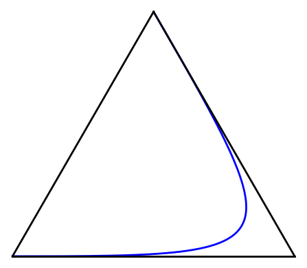
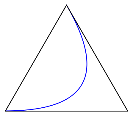
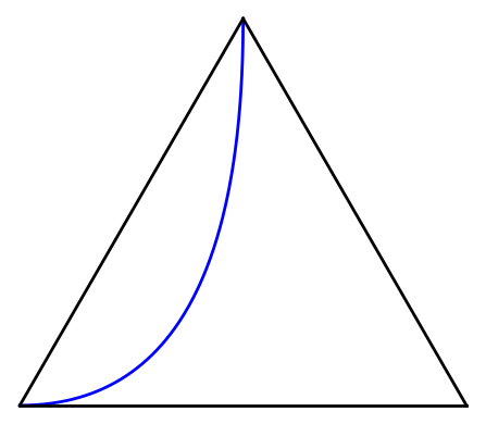
Figure 2. Fundamental models in $\Delta_{2}$. These correspond to the parametrizations $t\mapsto((1-t)^{3},3t(1-t),t^{3})$, $t\mapsto((1-t)^{2},2(1-t)t,t^{2})$, and $t\mapsto((1-t),t(1-t),t^{2}),$ from left to right. Their places are {(0,3), (1,1), (3,0)}, {(0,2), (1,1), (2,0)}, and {(0,1), (1,1), (2,0)}, respectively. In $\Delta_{2}$ there is a further fundamental model at the place {(0,2),(1,0),(1,1)}, but it is identical to the third model in this picture after a permutation of the coordinates of $\Delta_{n}$ and the reparametrization $t\mapsto 1-t$.

As for non-reduced models, there are up to coordinate permutations only two linear embeddings $\Delta_{1}\to\Delta_{2}$ of the form (1) or (2) that can be used to construct $\mathcal{M}$ from $\mathcal{M}_{0}$. These can vary with the parameter $\lambda$ and are reported in Figure 3 for $\lambda=1/3$.

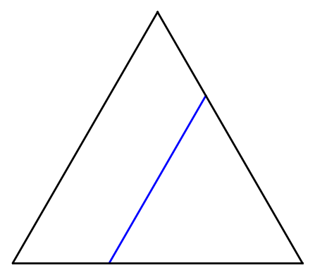
Figure 3. Non-reduced models in $\Delta_{2}.$ These arise from linear embeddings $\Delta_{1}\to\Delta_{2}$ of type (1) and (2), respectively. They are given by $t\mapsto((1-\lambda)t,\lambda,(1-\lambda)(1-t))$ and $t\mapsto((1-t),\lambda t,(1-\lambda)t)$, where $\lambda:=1/3.$ All other non-reduced one-dimensional models of ML degree one in $\Delta_{2}$ arise from these two by varying $\lambda$ and permuting the coordinates of $\Delta_{2}$.

3. Properties of chipsplitting games

We begin this section with the general definition of a (directed) chipsplitting game. Let $(V,E)$ be a directed graph without loops.

Definition 3.1.

Let $V^{\prime}\subseteq V$ be the subset of vertices with $\geq 1$ outgoing edge.

1. A chip configuration is a vector $w=(w_{v})_{v\in V}\in\operatorname{\mathbb{Z}}^{V}$ such that $\#\{v\in V\mid w_{v}\neq 0\}<\infty$.

2. The initial configuration is the zero vector $0\in\operatorname{\mathbb{Z}}^{V}$.

3. A splitting move at $p\in V$ maps a chip configuration $w=(w_{v})_{v\in V}$ to the chip configuration $\widetilde{w}=(\widetilde{w}_{v})_{v\in V}$ defined by

   $$\widetilde{w}_{v}:=\left\{\begin{array}[]{cl}w_{v}-1&\mbox{if $v=p$,}\\ w_{v}+1&\mbox{if $(p,v)\in E$, i.e., $E$ contains an edge from $p$ to $v$,}\\ w_{v}&\mbox{otherwise.}\end{array}\right.$$

   An unsplitting move at $p$ maps $\widetilde{w}$ back to $w$.

4. A chipsplitting game $f$ is a finite sequence of splitting and unsplitting moves. The outcome of $f$ is the chip configuration obtained from the initial configuration after executing all the moves in $f$.

5. A (chipsplitting) outcome is the outcome of any chipsplitting game.

Note that the moves in our game are all reversible and commute with each other. In particular, the order of the moves in a game does not matter and every outcome is the outcome of a game such that at no point in $V$ both a splitting and an unsplitting move occurs. We call games that have this property reduced. We usually assume chipsplitting games are reduced. The map

$$\{\mbox{reduced chipsplitting games on }(V,E)\}/\sim \to \{g\colon V^{\prime}\to\operatorname{\mathbb{Z}}\mid\#\{p\in V^{\prime}\mid g(p)\neq 0\}<\infty\}$$

$$f \mapsto \left(p\mapsto\mbox{number of moves at }p\mbox{ in }f\right)$$

is a bijection, where we count unsplitting moves negatively and consider two games $f,g$ equivalent if they are the same up to reordering. We identify a reduced chipsplitting game $f$ with its corresponding function $V^{\prime}\to\operatorname{\mathbb{Z}}$. The outcome $w=(w_{v})_{v\in V}$ of $f$ now satisfies

$$w_{v}=-f(v)+\sum_{\begin{subarray}{c}p\in V^{\prime}\\ (p,v)\in E\end{subarray}}f(v),$$

where we write $f(v)=0$ when $v\not\in V^{\prime}$.

Remark 3.2.

Let $A$ be an abelian group. The definitions above naturally extend from $\operatorname{\mathbb{Z}}$ to $A$, i.e., to the setting where the number of chips at a point and number of times a move is repeated are both allowed to be any element of $A$. Here (resp. when $A=\operatorname{\mathbb{Q}},\operatorname{\mathbb{R}}$), we say that the chip configurations, chipsplitting games and outcomes are $A$-valued (resp. rational, real).

We now define the directed graphs $(V_{d},E_{d})$ we consider in this paper. For $d\in\operatorname{\mathbb{N}}\cup\{\infty\}$, write

$$V_{d} := \{(i,j)\in\operatorname{\mathbb{Z}}_{\geq 0}^{2}\mid\deg(i,j)\leq d\},$$

$$E_{d} := \{(v,v+e)\mid v\in V_{d-1},e\in\{(1,0),(0,1)\}\},$$

where $\deg(i,j):=i+j$ is the degree of $(i,j)\in\operatorname{\mathbb{Z}}_{\geq 0}^{2}$.

Example 3.3.

We depict a chip configuration $w=(w_{i,j})_{(i,j)\in V_{d}}\in\operatorname{\mathbb{Z}}^{V_{d}}$ as a triangle of numbers with $w_{i,j}$ being the number in the $i$th column from the left and $j$th row from the bottom.

·           ·            ·           ·           1           1           1 · ·         · ·          · ·         1 ·         · 1         · 1         · · · · ·       1 · ·        1 1 ·       · 2 ·       · 2 ·       · 2 1       · 3 · 0 · · ·    -1 1 · ·     -1 · 1 ·    -1 · 1 ·    -1 · 1 ·    -1 · · 1    -1 · · 1

When $w_{i,j}=0$, we usually write · at position $(i,j)$ instead of 0. In the examples above, we have $d=3$. The leftmost configuration is the initial configuration. From left to right, we obtain the next five configurations by successively executing splitting moves at $(0,0)$, $(1,0)$, $(0,1)$, $(0,2)$, and $(2,0)$, respectively. Finally, we obtain the rightmost configuration by applying an unsplitting move at $(1,1)$.

Definition 3.4.

Let $w=(w_{i,j})_{(i,j)\in V_{d}}$ be a chip configuration.

1. The positive support of $w$ is $\operatorname{supp}^{+}(w):=\{(i,j)\in V_{d}\mid w_{i,j}>0\}$.

2. The negative support of $w$ is $\operatorname{supp}^{-}(w):=\{(i,j)\in V_{d}\mid w_{i,j}<0\}$.

3. The support of $w$ is $\operatorname{supp}(w):=\{(i,j)\in V_{d}\mid w_{i,j}\neq 0\}=\operatorname{supp}^{+}(w)\cup\operatorname{supp}^{-}(w)$.

4. The degree of $w$ is $\deg(w):=\max\{\deg(i,j)\mid(i,j)\in\operatorname{supp}(w)\}$.

5. We say that $w$ is valid when $\operatorname{supp}^{-}(w)\subseteq\{(0,0)\}$.

6. We say that $w$ is weakly valid when for all $(i,j)\in\operatorname{supp}^{-}(w)$ one of the following holds:

   1. $0\leq i,j\leq 3$,

   2. $0\leq i\leq 3$ and $\deg(i,j)\geq d-3$, or

   3. $0\leq j\leq 3$ and $\deg(i,j)\geq d-3$.

Figure 4 illustrates the notion of a weakly valid outcome, which will first be used in Section 6.5.

Figure 4. The corners of the four-entries wide outer ring of the triangle $V_{d}$. A chip configuration is weakly valid if its negative support is contained in the orange area.

We can now state our main conjecture and result in the language of valid outcomes.

Conjecture 3.5 (Boundedness for outcomes).

text

1. There exists a function $d\colon\operatorname{\mathbb{N}}\to\operatorname{\mathbb{N}}$ such that $\deg(w)\leq d(n)$ for all integers $n\in\operatorname{\mathbb{N}}$ and all valid outcomes $w$ with a positive support of size $n+1$.

2. We have $\deg(w)\leq 2\cdot\#\operatorname{supp}^{+}(w)-3$ for all valid outcomes $w$.

Theorem 3.6 (Degree bound for outcomes).

Conjecture 3.5(b) holds for all valid outcomes $w$ such that $\#\operatorname{supp}^{+}(w)\leq 5$.

We will prove Theorem 3.6 in Sections 5–7 (See Theorems  5.14, 6.21 and 7.2).

Conjecture 3.5 and Theorem 3.6 are equivalent to Conjecture 1.1 and Theorem 1.2, respectively. We will prove this in Section 4. Next, we again give the family of examples showing that part (b) of the conjecture would be sharp.

Proposition 3.7.

Suppose that $d=2k+1$ for some integer $k\geq 0$. Let the chip configuration $w=(w_{i,j})_{(i,j)\in V_{d}}\in\operatorname{\mathbb{Z}}^{V_{d}}$ be defined by $w_{0,0}=-1$, $w_{2k+1,0}=1$,

$$w_{k-i,2i+1}=\frac{2k+1}{2i+1}\binom{k+i}{2i}$$

for $i\in\{0,1,\ldots,k\}$ and $w_{i,j}=0$ otherwise. Then $w$ is a valid outcome.

Proof.

This follows from Proposition 2.5 and Lemma 4.2. ∎

Figure 5 illustrates the support of such an outcome for $d=7$.

* · · · * · · · · · · · * · · · · · · · · · · · * · · · * · · · · · · *

Figure 5. Support of the valid outcome defined in Proposition 3.7 for $d=7$.

Proposition 3.8.

Let $w$ be the outcome of a reduced chipsplitting game $f$. If $p\in V_{d-1}$ is a point with $\deg(p)\geq\deg(w)$, then $f$ does not contain any moves at $p$.

Proof.

Let $e:=\max\{\deg(i,j)\mid(i,j)\in V_{d-1},f(i,j)\neq 0\}$ be the maximal degree of a point $(i,j)\in V_{d-1}$ such that $f$ contains a move at $(i,j)$. For $k=0,\ldots,e$, let $n_{k}:=f(k,e-k)$ be the number of moves at $(k,e-k)$ in $f$, where we count unsplitting moves negatively. Now we see that

$$(w_{0,e+1},w_{1,e},\ldots,w_{e,1},w_{e+1,0})=(n_{0},n_{0}+n_{1},\ldots,n_{e-1}+n_{e},n_{e})$$

and $w_{i,j}=0$ for all $(i,j)\in V_{d}$ with $\deg(i,j)>e+1$. Since $(n_{0},\ldots,n_{e})\neq(0,\ldots,0)$, we see that $w_{i,j}\neq 0$ for some $(i,j)\in V_{d}$ with $\deg(i,j)=e+1$. Hence $\deg(w)=e+1$ and therefore $f$ does not contain any moves at any $p\in V_{d-1}$ with $\deg(p)\geq\deg(w)$. ∎

Remark 3.9.

Let $w\in\operatorname{\mathbb{Z}}^{V_{d}}$ be a chip configuration. Then $\deg(w)\leq d$. For all integers ${0\leq e\leq d}$, the map $(w_{i,j})_{(i,j)\in V_{d}}\mapsto(w_{i,j})_{(i,j)\in V_{e}}$ is a bijection between degree-$\leq$$e$ chip configurations on $(V_{d},E_{d})$ and chip configurations on $(V_{e},E_{e})$. Proposition 3.8 shows that this bijection restricts to a bijection between degree-$\leq$$e$ outcomes on $(V_{d},E_{d})$ and outcomes on $(V_{e},E_{e})$. In particular, the space of outcomes on $(V_{\infty},E_{\infty})$ is the direct limit of the spaces of outcomes on $(V_{d},E_{d})$ over all $d<\infty$.

3.1. Chipfiring games

The notion of chipsplitting games is inspired by that of chipfiring games. This subsection provides some background and explains this connection. For a thorough treatment of chipfiring games, see [5]. For the arguments in the rest of this article, we shall continue to use chipsplitting games.

Definition 3.10.

Let $(V,E)$ be a directed graph without loops.

1. Let $p\in V$ be a point with $k\geq 1$ outgoing edges. A firing move at $p$ maps a chip configuration $w=(w_{v})_{v\in V}$ to the chip configuration $\widetilde{w}=(\widetilde{w}_{v})_{v\in V}$ defined by

   $$\widetilde{w}_{v}:=\left\{\begin{array}[]{cl}w_{v}-k&\mbox{if $v=p$,}\\ w_{v}+1&\mbox{if $(p,v)\in E$,}\\ w_{v}&\mbox{otherwise.}\end{array}\right.$$

   An unfiring move at $p$ maps $\widetilde{w}$ back to $w$.

2. A chipfiring game $f$ is a finite sequence of firing and unfiring moves. The outcome of $f$ is the chip configuration obtained from the initial configuration after executing all the moves in $f$.

3. A chipfiring outcome is the outcome of any chipfiring game.

Remark 3.11.

For chipfiring games on finite undirected graphs, there is no need to define unfiring moves as an unfiring move at a point $p\in V$ equals the result of firing all other points $q\in V\setminus\{p\}$.

For our directed graphs $(V_{d},E_{d})$, we in fact have a natural bijection of its sets of chipsplitting and chipfiring outcomes in the rational setting. A $\operatorname{\mathbb{Q}}$-valued chip configuration is an outcome if and only if it equals a $\operatorname{\mathbb{Z}}$-valued outcome up to scaling. This means that chipfiring and chipsplitting games are essentially equivalent in our setting. However, chipsplitting games relate more directly to our statistical models as explained in Section 2.

Proposition 3.12.

The map

$$\phi\colon\{\text{\rm rational chipfiring outcomes on }(V_{d},E_{d})\} \to \{\text{\rm rational chipsplitting outcomes on }(V_{d},E_{d})\}$$

$$(w_{i,j})_{(i,j)\in V_{d}} \mapsto (2^{\deg(i,j)}w_{i,j})_{(i,j)\in V_{d}}$$

is a bijection.

Proof.

Let $w=(w_{i,j})_{(i,j)\in V_{d}}$ be the outcome of a chipfiring game $f\colon V_{d-1}\to\operatorname{\mathbb{Q}}$ and let $g\colon V_{d-1}\to\operatorname{\mathbb{Q}}$ be defined by $g(i,j)=2^{\deg(i,j)+1}f(i,j)$. Then we see that

$$2^{\deg(i,j)}w_{i,j}=2^{\deg(i,j)}\left(f(i-1,j)+f(i,j-1)-2f(i,j)\right)=g(i-1,j)+g(i,j-1)-g(i,j)$$

where $f(i,-1)=f(-1,j)=0$ for all $i,j$. So we see that $\phi(w)$ is the outcome of the chipsplitting game $g$. Hence $\phi$ is well-defined. The map $\phi$ is clearly injective. When $w^{\prime}$ is the outcome of a chipsplitting game $g$, then $w^{\prime}=\phi(w)$ where $w$ is the outcome of the chipfiring game $f$ defined by $f(i,j)=2^{-\deg(i,j)-1}g(i,j)$. So $\phi$ is a bijection. ∎

Remark 3.13.

Several problems concerning chipfiring are studied by defining a notion of energy for a configuration. In our setting

$$E(w):=\frac{1}{2}\sum_{(i,j)\in V_{d}}\deg(i,j)w_{i,j}.$$

would be one possible way to define it. One can show that if $w$ is the outcome of a chipfiring game $f$, then $E(w)$ equals the number of moves in $f$, where we count unfiring moves negatively. Since all moves in our games are reversable, we do not expect this notion to be useful for our purposes.

We now return to the setting of chipsplitting games.

3.2. Symmetry

For every $d\in\operatorname{\mathbb{N}}\cup\{\infty\}$, define an action of the group $S_{2}=\langle(12)\rangle$ on $\operatorname{\mathbb{Z}}^{V_{d}}$ by setting

$$(12)\cdot(w_{i,j})_{(i,j)\in V_{d}}:=(w_{j,i})_{(i,j)\in V_{d}},$$

where clearly $(12)\cdot((12)\cdot w))=w$ for all $w\in\operatorname{\mathbb{Z}}^{V_{d}}$. We also let $S_{2}$ act on $V_{d}$ by $(12)\cdot(i,j):=(j,i)$.

The initial configuration is fixed by $S_{2}$. Let $w\in\operatorname{\mathbb{Z}}^{V_{d}}$, $p\in V_{d-1}$, and let $\widetilde{w}$ be the result of applying an (un)splitting move at $p$ to $w$. Then $(12)\cdot\widetilde{w}$ is the result of applying an (un)splitting move at $(12)\cdot p$ to $(12)\cdot w$. So we see that if $w$ is the outcome of a reduced chipsplitting game $f$, then $(12)\cdot w$ is the outcome of the chipsplitting game $(i,j)\mapsto f(j,i)$. Hence the space of outcomes is closed under the action of $S_{2}$. Let $w\in\operatorname{\mathbb{Z}}^{V_{d}}$ be a chip configuration. Then

$$\operatorname{supp}^{+}((12)\cdot w) =(12)\cdot\operatorname{supp}^{+}(w), \operatorname{supp}^{-}((12)\cdot w) =(12)\cdot\operatorname{supp}^{-}(w),$$

$$\operatorname{supp}((12)\cdot w) =(12)\cdot\operatorname{supp}(w), \deg((12)\cdot w) =\deg(w).$$

Furthermore, $w$ is (weakly) valid if and only if $(12)\cdot w$ is (weakly) valid.

3.3. Pascal equations

Another way to study the space of outcomes is via the set of linear forms that vanish on it. A linear form on $\operatorname{\mathbb{Z}}^{V_{d}}$ is a function $\operatorname{\mathbb{Z}}^{V_{d}}\to\operatorname{\mathbb{Z}}$ of the form

$$(w_{i,j})_{(i,j)\in V_{d}}\mapsto\sum_{(i,j)\in V_{d}}c_{i,j}w_{i,j},$$

which we will denote by $\sum_{(i,j)\in V_{d}}c_{i,j}x_{i,j}$. The group $S_{2}$ acts on the space of linear forms on $\operatorname{\mathbb{Z}}^{V_{d}}$ via

$$(12)\cdot\sum_{(i,j)\in V_{d}}c_{i,j}x_{i,j}:=\sum_{(i,j)\in V_{d}}c_{j,i}x_{i,j}.$$

Definition 3.14.

We say that a linear form $\sum_{(i,j)\in V_{d}}c_{i,j}x_{i,j}$ is a Pascal equation when

$$c_{i,j}=c_{i+1,j}+c_{i,j+1}$$

for all $(i,j)\in V_{d-1}$.

This terminology is inspired by the Pascal triangle, whose entries satisfy the same condition. The space of Pascal equations is closed under the action of $S_{2}$.

Proposition 3.15.

Let $(a_{k})_{k=0}^{d}\in\operatorname{\mathbb{Z}}^{\operatorname{\mathbb{N}}_{\leq d}}$ be any vector.

1. There exists a unique Pascal equation $\sum_{(i,j)\in V_{d}}c_{i,j}x_{i,j}$ such that $c_{0,j}=a_{j}$ for all $0\leq j\leq d$.

2. There exists a unique Pascal equation $\sum_{(i,j)\in V_{d}}c_{i,j}x_{i,j}$ such that $c_{i,0}=a_{i}$ for all $0\leq i\leq d$.

Proof.

(a) Set $c_{0,j}:=a_{j}$ for all integers $0\leq j\leq d$ and define

$$c_{i+1,j}:=c_{i,j}-c_{i,j+1}$$

for all $(i,j)\in V_{d}$ via recursion on $i>0$. Then $\sum_{(i,j)\in V_{d}}c_{i,j}x_{i,j}$ is a Pascal equation such that $c_{0,j}=a_{j}$ for all integers $0\leq j\leq d$. Clearly, it is the only Pascal equation with this property.

(b) Write

$$(12)\cdot\sum_{(i,j)\in V_{d}}c_{i,j}x_{i,j}=\sum_{(i,j)\in V_{d}}d_{i,j}x_{i,j}.$$

Then $c_{k,0}=a_{k}$ if and only if $d_{0,k}=a_{k}$ and hence the statement follows from (a). ∎

Our next goal is to prove that a chip configuration is an outcome if and only if all Pascal equations vanish at it.

Proposition 3.16.

Let $w\in\operatorname{\mathbb{Z}}^{V_{d}}$ be a chip configuration. Then the value at $w$ of any given Pascal equation on $\operatorname{\mathbb{Z}}^{V_{d}}$ is invariant under (un)splitting moves. In particular, all Pascal equations on $\operatorname{\mathbb{Z}}^{V_{d}}$ vanish at all outcomes.

Proof.

Let $w=(w_{i,j})_{(i,j)\in V_{d}}$ be a chip configuration and suppose we obtain $\widetilde{w}=(\widetilde{w}_{i,j})_{(i,j)\in V_{d}}$ from $w$ by applying a chipsplitting move at $(i^{\prime},j^{\prime})\in V_{d-1}$. Let $\sum_{(i,j)\in V_{d}}c_{i,j}x_{i,j}$ be a Pascal equation. Then we see that

$$\sum_{(i,j)\in V_{d}}c_{i,j}\widetilde{w}_{i,j}=\sum_{(i,j)\in V_{d}}c_{i,j}\left\{\begin{array}[]{cl}w_{i,j}-1&\mbox{if $(i,j)=(i^{\prime},j^{\prime})$,}\\ w_{i,j}+1&\mbox{if $(i,j)=(i^{\prime}+1,j)$,}\\ w_{i,j}+1&\mbox{if $(i,j)=(i^{\prime},j^{\prime}+1)$,}\\ w_{i,j}&\mbox{otherwise}\end{array}\right\}=\sum_{(i,j)\in V_{d}}c_{i,j}w_{i,j}$$

since $c_{i^{\prime}+1,j^{\prime}}+c_{i^{\prime},j^{\prime}+1}-c_{i^{\prime},j^{\prime}}=0$, which proves the first claim. For the second claim it suffices to note that all Pascal equations vanish at the initial configuration. ∎

Let $w=(w_{i,j})_{(i,j)\in V_{d}}$ be a degree-$e$ chip configuration. Then there exists a unique reduced chipsplitting game that uses only moves at $(i,j)\in V_{d-1}$ with $\deg(i,j)=e-1$ and that sets the values $w_{0,e},w_{1,e-1},\ldots,w_{e-1,1}$ to $0$. Note that these moves do not alter the alternating sum $\sum_{k=0}^{e}(-1)^{k}w_{k,e-k}$. So, if $\sum_{k=0}^{e}(-1)^{k}w_{k,e-k}=0$, this chipsplitting game also sets $w_{e,0}$ to $0$. This motivates the following definition.

Definition 3.17.

Let $w=(w_{i,j})_{(i,j)\in V_{d}}$ be a degree-$e$ chip configuration such that

$$\sum_{k=0}^{e}(-1)^{k}w_{k,e-k}=0.$$

The retraction of $w$ is the unique chip configuration obtained from $w$ using moves at points $(i,j)\in V_{d-1}$ with $\deg(i,j)=e-1$ such that $\deg(w)<e$.

Proposition 3.18.

Let $w=(w_{i,j})_{(i,j)\in V_{d}}$ be a degree-$e$ chip configuration. Then $w$ is an outcome if and only if $\sum_{k=0}^{e}(-1)^{k}w_{k,e-k}=0$ and the retraction of $w$ is an outcome.

Proof.

If $\sum_{k=0}^{e}(-1)^{k}w_{k,e-k}=0$, then $w$ and its retraction are obtained from each other using finite sequences of moves. So it suffices to prove that $\sum_{k=0}^{e}(-1)^{k}w_{k,e-k}=0$ holds when $w$ is an outcome. Assume that $w$ is the outcome of a reduced chipsplitting game $f$. Then $e-1$ is the maximal degree of a point in $V_{d-1}$ at which a move in $f$ occured. As moves at $(i,j)$ preserve the value of $\sum_{k=0}^{e}(-1)^{k}w_{k,e-k}$ for all $(i,j)\in V_{d-1}$ with $\deg(i,j)\leq e-1$, we see that $\sum_{k=0}^{e}(-1)^{k}w_{k,e-k}=0$. ∎

Proposition 3.19.

Let $w\in\operatorname{\mathbb{Z}}^{V_{d}}$ be a chip configuration and suppose that all Pascal equation on $\operatorname{\mathbb{Z}}^{V_{d}}$ vanish at $w$. Then $w$ is an outcome.

Proof.

By Proposition 3.15, for every integer $0\leq e\leq d$ there exists a Pascal equation

$$\phi^{(e)}:=\sum_{(i,j)\in V_{d}}c^{(e)}_{i,j}x_{i,j}$$

with $c^{(e)}_{0,j}=0$ for $j<e$ and $c^{(e)}_{0,e}=1$. Note that $c^{(e)}_{i,j}=0$ for all $(i,j)\in V_{d}$ with $\deg(i,j)<e$ and $c^{(e)}_{k,e-k}=(-1)^{k}$ for $k\in\{0,\ldots,e\}$. Next, note that for $e=\deg(w)$ we have

$$\sum_{k=0}^{e}(-1)^{k}w_{i,j}=\phi^{(e)}(w)=0$$

and hence $w$ has a retraction $w^{\prime}$, at which all Pascal equations also vanish. Repeating the same argument, we see that $w^{\prime}$ also has a retraction $w^{\prime\prime}$, at which all Pascal equations again vanish. After repeating this $e+1$ times, we arrive at a chip configuration of degree $<0$, which must be the initial configuration. Hence by Proposition 3.18, we see that $w$ is an outcome. ∎

Definition 3.20.

Let $0\leq k\leq d$ be an integer.

1. We write $\psi_{k}$ for the unique Pascal equation $\sum_{(i,j)\in V_{d}}c_{i,j}x_{i,j}$ such that $c_{0,j}=\delta_{jk}$

2. We write $\overline{\psi}_{k}:=(12)\cdot\psi_{k}$.

Proposition 3.21.

1. We have

   $$\psi_{k}=(-1)^{k}\sum_{(i,j)\in V_{d}}(-1)^{j}\binom{i}{k-j}x_{i,j}\mbox{ and }\overline{\psi}_{k}=(-1)^{k}\sum_{(i,j)\in V_{d}}(-1)^{i}\binom{j}{k-i}x_{i,j}$$

   for all integers $0\leq k\leq d$.

2. Every Pascal equation can be written uniquely as

   $$\sum_{k=0}^{d}a_{k}\psi_{k}=\sum_{k=0}^{d}b_{k}\overline{\psi}_{k},$$

   where $a_{k},b_{k}\in\operatorname{\mathbb{Z}}$. When $d<\infty$, the $\psi_{k}$ and $\overline{\psi}_{k}$ form two bases of the space of Pascal equations.

Proof.

(a) We have $(-1)^{k+j}\binom{0}{k-j}=\delta_{jk}$ and so it suffices to prove that

$$\sum_{(i,j)\in V_{d}}(-1)^{j}\binom{i}{k-j}x_{i,j}$$

is in fact a Pascal equation. Indeed, we have

$$(-1)^{j}\binom{i}{k-j}=(-1)^{j}\binom{i+1}{k-j}+(-1)^{j+1}\binom{i}{k-(j+1)}$$

for all $(i,j)\in V_{d}$ as $\binom{a+1}{b+1}=\binom{a}{b+1}+\binom{a}{b}$ for all integers $a,b$.

(b) Write

$$\sum_{(i,j)\in V_{d}}c_{i,j}x_{i,j}=\sum_{k=0}^{d}a_{k}\psi_{k}=\sum_{k=0}^{d}b_{k}\overline{\psi}_{k}.$$

Then we see that

$$c_{i,j}=\sum_{k=j}^{\deg(i,j)}a_{k}(-1)^{k+j}\binom{i}{k-j}=\sum_{k=i}^{\deg(i,j)}b_{k}(-1)^{k+i}\binom{j}{k-i}$$

for all $(i,j)\in V_{d}$. We see that each $c_{i,j}$ is a finite sum. We also see that $c_{0,j}=a_{j}$ and $c_{i,0}=b_{i}$ for all $i,j\in\operatorname{\mathbb{N}}_{\leq d}$. So now the statement follows from Proposition 3.15. ∎

Example 3.22.

For $d=7$ and $k=3$, the Pascal equation $\psi_{k}$ can be visualised by writing the coefficients $c_{i,j}$ on the grid $V_{d}$ as follows:

· ·  · ·  ·  · ·  ·  ·  · 1  1  1  1  1 · -1 -2 -3 -4  -5 ·  ·  1  3  6  10  15 ·  ·  · -1 -4 -10 -20 -35

We note that the signs of the rows alternate and that $|c_{i,j}|=|c_{i-1,j}|+|c_{i-1,j+1}|$ for all $i>0$.

3.4. Additional structure for $d<\infty$

In this subsection, we assume that $d<\infty$. By Proposition 3.21, we know that the $\psi_{k}$ and $\overline{\psi}_{k}$ form two bases of the space of Pascal equations on $\operatorname{\mathbb{Z}}^{V_{d}}$. When $d<\infty$, we also have another natural basis.

Proposition 3.23.

For every vector $(a_{0},\ldots,a_{d})\in\operatorname{\mathbb{Z}}^{d+1}$, there exists a unique Pascal equation

$$\sum_{(i,j)\in V_{d}}c_{i,j}x_{i,j}$$

such that $c_{k,d-k}=a_{k}$ for all integers $0\leq k\leq d$.

Proof.

Let $(a_{0},\ldots,a_{d})\in\operatorname{\mathbb{Z}}^{d+1}$, set $c_{k,d-k}:=a_{k}$ for $k\in\{0,\ldots,d\}$ and, for $e=d-1,\ldots,0$, set $c_{k,e-k}=c_{k+1,e-k}+c_{k,e-k+1}$ for $k\in\{0,\ldots,e\}$ recursively. Then

$$\sum_{(i,j)\in V_{d}}c_{i,j}x_{i,j}$$

is a Pascal equation such that $c_{k,d-k}=a_{k}$ for all integers $0\leq k\leq d$. Clearly, this Pascal equation is unique with this property. ∎

Definition 3.24.

Let $(a,b)\in V_{d}$ with $\deg(a,b)=d$. We write $\varphi_{a,b}$ for the unique Pascal equation $\sum_{(i,j)\in V_{d}}c_{i,j}x_{i,j}$ such that $c_{i,j}=\delta_{ia}$ (or equivalently $c_{i,j}=\delta_{jb}$) for all $(i,j)\in V_{d}$ with $\deg(i,j)=d$.

Proposition 3.25.

1. We have

   $$\varphi_{a,b}=\sum_{(i,j)\in V_{d}}\binom{d-(i+j)}{a-i}x_{i,j}=\sum_{(i,j)\in V_{d}}\binom{d-(i+j)}{b-j}x_{i,j}$$

   for all $(a,b)\in V_{d}$ with $\deg(a,b)=d$.

2. The $\varphi_{a,b}$ form a basis for the space of all Pascal equations.

Proof.

(a) We have

$$\delta_{ia}=\binom{d-(i+j)}{a-i}=\binom{d-(i+j)}{b-j}=\delta_{jb}$$

for all $(i,j)\in V_{d}$ with $\deg(i,j)=d$. So it suffices to show that

$$\sum_{(i,j)\in V_{d}}\binom{d-(i+j)}{a-i}x_{i,j}$$

is a Pascal equation. Indeed, we have

$$\binom{d-(i+j)}{a-i}=\binom{d-(i+1+j)}{a-(i+1)}+\binom{d-(i+j+1)}{a-i}$$

for all $(i,j)\in V_{d-1}$ as $\binom{a+1}{b+1}=\binom{a}{b+1}+\binom{a}{b}$ for all integers $a,b$.

(b) Every Pascal equation can be uniquely written as

$$\sum_{(i,j)\in V_{d}}c_{i,j}x_{i,j}=\sum_{(a,b)\in V_{d}\setminus V_{d-1}}c_{a,b}\varphi_{a,b}.$$

So we see that the $\varphi_{a,b}$ form a basis for the space of all Pascal equations. ∎

Example 3.26.

For $d=7$ and $(a,b)=(3,4)$, the Pascal equation $\varphi_{a,b}$ can be visualised by writing the coefficients $c_{i,j}$ on the grid $V_{d}$ as follows:

 ·  ·  ·  ·  ·  ·  1  1  1  1  4  3  2  1  · 10  6  3  1  ·  · 20 10  4  1  ·  ·  · 35 15  5  1  ·  ·  ·  ·

We note that the coefficients form a Pascal triangle.

Next we define an action of $S_{3}=\langle(12),(123)\rangle$ on $\operatorname{\mathbb{Z}}^{V_{d}}$. We set

$$(12)\cdot(w_{i,j})_{(i,j)\in V_{d}} := (w_{j,i})_{(i,j)\in V_{d}}=:w^{(a)}$$

$$(123)\cdot(w_{i,j})_{(i,j)\in V_{d}} := ((-1)^{d-j}w_{j,d-\deg(i,j)})_{(i,j)\in V_{d}}=:w^{(b)}$$

for all $w=(w_{i,j})_{(i,j)\in V_{d}}\in\operatorname{\mathbb{Z}}^{V_{d}}$. We now verify that this defines an action of $S_{3}$ on the set of outcomes by calculating

$$(12)\cdot w^{(a)} = w$$

$$(123)\cdot w^{(b)} = ((-1)^{d-j}w^{(b)}_{j,d-\deg(i,j)})_{(i,j)\in V_{d}}=((-1)^{d-i}w_{d-\deg(i,j),i})_{(i,j)\in V_{d}}=:w^{(bb)}$$

$$(123)\cdot w^{(bb)} = ((-1)^{d-j}w^{(bb)}_{j,d-\deg(i,j)})_{(i,j)\in V_{d}}=w$$

$$(12)\cdot w^{(b)} = (w^{(b)}_{j,i})_{(i,j)\in V_{d}}=((-1)^{d-i}w_{i,d-\deg(i,j)})_{(i,j)\in V_{d}}:=w^{(ab)}$$

$$(123)\cdot w^{(ab)} = ((-1)^{d-j}w^{(ab)}_{j,d-\deg(i,j)})_{(i,j)\in V_{d}}=w^{(a)}$$

and deducing

$$(12)\cdot((12)\cdot w) =(12)\cdot w^{(a)}=w,$$

$$(123)\cdot((123)\cdot((123)\cdot w)) =(123)\cdot((123)\cdot w^{(b)})=(123)\cdot w^{(bb)}=w,$$

$$(12)\cdot((123)\cdot((12)\cdot((123)\cdot w))) =(12)\cdot((123)\cdot((12)\cdot w^{(b)}))=(12)\cdot\!((123)\cdot w^{(ab)})=(12)\cdot w^{(a)}=w$$

for all $w=(w_{i,j})_{(i,j)\in V_{d}}\in\operatorname{\mathbb{Z}}^{V_{d}}$. Hence the action is well-defined. We have

$$(13)\cdot(w_{i,j})_{(i,j)\in V_{d}} = ((-1)^{d-j}w_{d-\deg(i,j),j})_{(i,j)\in V_{d}}$$

$$(23)\cdot(w_{i,j})_{(i,j)\in V_{d}} = ((-1)^{d-i}w_{i,d-\deg(i,j)})_{(i,j)\in V_{d}},$$

$$(132)\cdot(w_{i,j})_{(i,j)\in V_{d}} = ((-1)^{d-i}w_{d-\deg(i,j),i})_{(i,j)\in V_{d}}.$$

The way $(12)$, $(13)$ and $(23)$ act is vizualized below. The permutation $(12)$ switches the order of all entries of the same degree. The permutation $(13)$ switches the order of all entries of the same row and changes the signs of alternating rows. Similarly, the permutation $(23)$ switches the order of all entries of the same column and changes the signs of alternating columns.

       

Note that the set of weakly valid chip configurations is closed under the action of $S_{3}$. The same is true for the space of outcomes.

Proposition 3.27.

The space of outcomes is closed under the action of $S_{3}$.

Proof.

Let $w=(w_{i,j})_{(i,j)\in V_{d}}$ be an outcome. We already know that $(12)\cdot w$ is again an outcome. So it suffices to prove that $(123)\cdot w$ is an outcome as well. This is indeed the case since

$$\psi_{k}((123)\cdot w) = (-1)^{k}\sum_{(i,j)\in V_{d}}(-1)^{j}\binom{i}{k-j}(-1)^{d-j}w_{j,d-\deg(i,j)}$$

$$= (-1)^{d-k}\sum_{(i^{\prime},j^{\prime})\in V_{d}}\binom{d-(i^{\prime}+j^{\prime})}{k-i^{\prime}}w_{i^{\prime},j^{\prime}}$$

$$= (-1)^{d-k}\varphi_{k,d-k}(w)=0$$

for all integers $0\leq k\leq d$. ∎

We also define an action of $S_{3}$ on $V_{d}$. We set

$$(12)\cdot(i,j) :=(j,i), (123)\cdot(i,j) :=(d-\deg(i,j),i),$$

$$(13)\cdot(i,j) :=(d-\deg(i,j),j), (132)\cdot(i,j) :=(j,d-\deg(i,j)),$$

$$(23)\cdot(i,j) :=(i,d-\deg(i,j)),$$

for all $(i,j)\in V_{d}$. We have $\sigma\cdot\operatorname{supp}(w)=\operatorname{supp}(\sigma\cdot w)$ for all $w\in\operatorname{\mathbb{Z}}^{V_{d}}$ and $\sigma\in S_{3}$.

3.5. Valid outcomes

In this paper, we are mostly interested in valid outcomes, since they correspond to reduced models as explained in Section 4.

Lemma 3.28.

Let $w=(w_{i,j})_{(i,j)\in V_{d}}\in\operatorname{\mathbb{Z}}^{V_{d}}$ be an outcome and suppose that $\operatorname{supp}^{-}(w)=\emptyset$. Then $w$ is the initial configuration.

Proof.

We may assume that $d<\infty$. We have $w_{i,j}\geq 0$ for all $(i,j)\in V_{d}$. For every $(a,b)\in V_{d}$ of degree $d$, the equation $\varphi_{a,b}(w)=0$ shows that $w_{i,j}=0$ for all $i\in\{0,\ldots,a\}$ and $j\in\{0,\ldots,b\}$. Combined, this shows that $w_{i,j}=0$ for all $(i,j)\in V_{d}$. ∎

Proposition 3.29.

Let $w=(w_{i,j})_{(i,j)\in V_{d}}\in\operatorname{\mathbb{Z}}^{V_{d}}$ be an outcome and suppose that $\#\operatorname{supp}^{-}(w)=1$. Write $c_{0}=\min\{i\mid(i,j)\in V_{d}\mid w_{i,j}\neq 0\}$, $r_{0}=\min\{j\mid(i,j)\in V_{d}\mid w_{i,j}\neq 0\}$ and $d^{\prime}=d-c_{0}-r_{0}$. Then

$$(w_{c_{0}+i,r_{0}+j})_{(i,j)\in V_{d^{\prime}}}\in\operatorname{\mathbb{Z}}^{V_{d^{\prime}}}$$

is a valid outcome. In particular, if $c_{0}=r_{0}=0$, then $w$ is a valid outcome.

Proof.

We may assume that $d<\infty$. First we suppose that $c_{0}=r_{0}=0$. Then the equations $\varphi_{0,d}(w)=0$ and $\varphi_{d,0}(w)=0$ show that $w_{0,j}<0$ and $w_{i,0}<0$ for some $i,j\in\{0,\ldots,d\}$. Since $\#\operatorname{supp}^{-}(w)=1$, it follows that $i=j=0$ and $\operatorname{supp}^{-}(w)=\{(0,0)\}$. Hence $w$ is indeed valid.

In general, we note that $\varphi_{c_{0}+a,r_{0}+b}$ vanishes on $w$ for all $(a,b)\in V_{d^{\prime}}\setminus V_{d^{\prime}-1}$. So $\varphi_{a,b}$ vanishes on $(w_{c_{0}+i,r_{0}+j})_{(i,j)\in V_{d^{\prime}}}$ for all $(a,b)\in V_{d^{\prime}}\setminus V_{d^{\prime}-1}$. This means that $(w_{c_{0}+i,r_{0}+j})_{(i,j)\in V_{d^{\prime}}}$ is an outcome to which we can apply the previous case. ∎

Proposition 3.30.

Let $w=(w_{i,j})_{(i,j)\in V_{d}}$ be a valid outcome. If $w_{0,0}=0$, then $w$ is the initial configuration.

Proof.

This follows directly from Lemma 3.28. ∎

4. From reduced models to valid outcomes and back

Let $d\in\operatorname{\mathbb{N}}\cup\{\infty\}$, write $\deg(i,j):=i+j$ for $(i,j)\in\operatorname{\mathbb{Z}}_{\geq 0}^{2}$ and take $V_{d}:=\{(i,j)\in\operatorname{\mathbb{Z}}_{\geq 0}^{2}\mid\deg(i,j)\leq d\}$. Thus $V_{d}$ can be seen as a triangle of grid points.

Definition 4.1.

Define an integral (resp. rational, real) chip configuration to be an element $w=(w_{i,j})_{(i,j)\in V_{d}}$ of $\operatorname{\mathbb{Z}}^{V_{d}}$ (resp. $\operatorname{\mathbb{Q}}^{V_{d}}$, $\operatorname{\mathbb{R}}^{V_{d}}$) such that $\operatorname{supp}(w):=\{(i,j)\in V_{d}\mid w_{i,j}\neq 0\}$ is a finite set.

For $d^{\prime}\leq d$ we identify $\operatorname{\mathbb{Z}}^{V_{d^{\prime}}}$ (resp. $\operatorname{\mathbb{Q}}^{V_{d^{\prime}}},\operatorname{\mathbb{R}}^{V_{d^{\prime}}}$) with a subset of $\operatorname{\mathbb{Z}}^{V_{d}}$ (resp. $\operatorname{\mathbb{Q}}^{V_{d}},\operatorname{\mathbb{R}}^{V_{d}}$) by setting $w_{i,j}=0$ for all $i,j\in V_{d}\setminus V_{d^{\prime}}$. We define the positive support and negative support of $w$ to be

$$\operatorname{supp}^{+}(w):=\{(i,j)\in V_{\infty}\mid w_{i,j}>0\},\quad\operatorname{supp}^{-}(w):=\{(i,j)\in V_{\infty}\mid w_{i,j}<0\}$$

and we say that $w$ is valid when $\operatorname{supp}^{-}(w)\subseteq\{(0,0)\}$. We define the degree of $w$ to be

$$\deg(w):=\max\{\deg(i,j)\mid(i,j)\in\operatorname{supp}(w)\}.$$

In Section 3, we defined the notion of chipsplitting games and what it means for a chip configuration to be an outcome of such a game. In this section, we will use the following characterization.

Lemma 4.2.

The space of integral (resp. rational, real) outcomes equals the kernel of the linear map

$$\alpha_{d}\colon R^{V_{d}} \to R[t]_{\leq d}$$

$$(w_{i,j})_{(i,j)\in V_{d}} \mapsto \sum_{(i,j)\in V_{d}}w_{i,j}t^{i}(1-t)^{j}$$

where $R=\operatorname{\mathbb{Z}}$ (resp. $R=\operatorname{\mathbb{Q}},\operatorname{\mathbb{R}}$).

Proof.

For $d=\infty$, the map

$$\alpha_{d}\colon R^{V_{d}} \to R[t]_{\leq d}$$

$$(w_{i,j})_{(i,j)\in V_{d}} \mapsto \sum_{(i,j)\in V_{d}}w_{i,j}t^{i}(1-t)^{j}$$

is the direct limit of the maps $\alpha_{e}$ for $e<\infty$. So we may assume that $d<\infty$. In this case, we know that the space of outcomes has codimenion $d+1$ by Proposition 3.21(b). For a given polynomial $p=\sum_{j=0}^{d}c_{j}t_{j}\in R[t]_{\leq d}$, set $w_{i,j}=c_{i}$ when $j=0$ and $w_{i,j}=0$ otherwise. Then $\alpha_{d}(w_{i,j})_{(i,j)\in V_{d}}=p$. So we see that $\alpha_{d}$ is surjective. Hence the kernel of $\alpha_{d}$ has the same codimension as the space of outcomes. It now suffices to show that every outcome is contained in the kernel of $\alpha_{d}$. Note that the initial configuration is contained in the kernel of $\alpha_{d}$. And, for $w\in R^{V_{d}}$, the value of $\alpha_{d}(w)$ does not change when we execute a chipsplitting move at $(i,j)\in V_{d-1}$. Indeed, we have

$$-t^{i}(1-t)^{j}+t^{i+1}(1-t)^{j}+t^{i}(1-t)^{j+1}=t^{i}(1-t)^{j}(-1+t+(1-t))=0$$

and so every outcome is contained in the kernel of $\alpha_{d}$. ∎

Let $\mathcal{M}=(w_{\nu},i_{\nu},j_{\nu})_{\nu=0}^{n}$ be a reduced model. Then this model induces a real chip configuration $w(\mathcal{M})=(w_{i,j})_{(i,j)\in V_{\infty}}$ by setting

$$w_{i,j}:=\left\{\begin{array}[]{cl}-1&\mbox{if $(i,j)=(0,0)$,}\\ w_{\nu}&\mbox{if $(i,j)=(i_{\nu},j_{\nu})$,}\\ 0&\mbox{otherwise}\end{array}\right.$$

We have the following result.

Proposition 4.3.

text

1. The map

   $$\mathcal{M}\mapsto w(\mathcal{M})$$

   is a bijection between the set of reduced models and the set of valid real outcomes $w\in\operatorname{\mathbb{R}}^{V_{\infty}}$ with $w_{0,0}=-1$.

2. Let $S$ be the place of $\mathcal{M}$. Then $\operatorname{supp}^{+}(w(\mathcal{M}))=S$.

3. The map $\mathcal{M}\mapsto w(\mathcal{M})$ is degree-preserving.

4. The chip configuration $w(\mathcal{M})$ is rational if and only if the coefficients of $\mathcal{M}$ are all rational.

5. Every valid rational outcome $w\in\operatorname{\mathbb{Q}}^{V_{\infty}}$ is of the form $\lambda\hat{w}$ for some $\lambda\in\operatorname{\mathbb{Q}}_{>0}$ and valid integral outcome $\hat{w}\in\operatorname{\mathbb{Z}}^{V_{\infty}}$.

6. Let $w\in\operatorname{\mathbb{R}}^{V_{\infty}}$ be a valid real outcome with $w_{0,0}=0$. Then $w=0$.

Proof.

(a) From Lemma 4.2, it follows that $w(\mathcal{M})$ is indeed a valid real outcome with value $-1$ at $(0,0)$. Clearly, the map $\mathcal{M}\mapsto w(\mathcal{M})$ is injective. Let $w\in\operatorname{\mathbb{R}}^{V_{\infty}}$ be a valid real outcome with $w_{0,0}=-1$ and write $\operatorname{supp}^{+}(w)=\{(i_{0},j_{0}),\ldots,(i_{n},j_{n})\}$ and take $w_{\nu}:=w_{i_{\nu},j_{\nu}}$ for $\nu=0,\ldots,n$. Then $(w_{\nu},i_{\nu},j_{\nu})_{\nu=0}^{n}$ is a reduced model by Lemma 4.2. Hence the map $\mathcal{M}\mapsto w(\mathcal{M})$ is also surjective.

(b) This holds by the definition of $w(\mathcal{M})$.

(c) This holds since $\operatorname{supp}^{-}(w(\mathcal{M}))=\{(0,0)\}\cup\operatorname{supp}^{+}(w)=\{(0,0)\}\cup S$ for all reduced models $\mathcal{M}$.

(d) This holds by the definition of $w(\mathcal{M})$.

(e) For every valid rational outcome $w\in\operatorname{\mathbb{Q}}^{V_{\infty}}$ there exist an $n\in\operatorname{\mathbb{N}}$ such that $nw_{i,j}\in\operatorname{\mathbb{Z}}$ for all $(i,j)$ in the finite set $\operatorname{supp}(w)$. Take $\hat{w}:=nw$ and $\lambda:=1/n\in\operatorname{\mathbb{Q}}_{>0}$. Then $\hat{w}\in\operatorname{\mathbb{Z}}^{V_{\infty}}$ is an valid integral outcome using Lemma 4.2 and $w=\lambda\hat{w}$.

(f) Since $w$ is an outcome with $\operatorname{supp}^{-}(w)=\emptyset$, we know by Lemma 4.2 that

$$\sum_{(i,j)\in\operatorname{supp}^{+}(w)}w_{i,j}t^{i}(1-t)^{j}=\sum_{(i,j)\in V_{\infty}}w_{i,j}t^{i}(1-t)^{j}=0$$

and, by evaluating at $t=1/2$, we see that $\operatorname{supp}^{+}(w)$ can only be the empty set. Hence $w=0$. ∎

Proposition 4.4.

Conjectures 1.1 and 3.5 are equivalent. Theorems 1.2 and 3.6 are equivalent.

Proof.

By Remark 2.19, we know that for Conjecture 1.1 it suffices to only consider fundamental models. By Remark 2.13, we know that the coefficients of a fundamental model are rational. Hence for Conjecture 1.1 it also suffices to consider all reduced models with rational coefficients.

By Proposition 4.3(e), every valid rational outcome is a positive multiple of a valid integral outcome. The space of outcomes is closed under scaling, and scaling does not change the degree or size of the positive support of a chip configuration. Hence for Conjecture 3.5 we may also consider all valid rational outcomes $w$ with $w_{0,0}=-1$.

Now, by Proposition 4.3 we know that the map $\mathcal{M}\mapsto w(\mathcal{M})$ is a degree-preserving bijection between the set of reduced models in $\Delta_{n}$ with rational coefficients and the set of valid rational outcomes $w$ with $w_{0,0}=-1$ and $\#\operatorname{supp}^{+}(w)=n+1$. This shows the required equivalences. ∎

Next, we consider the chipsplitting equivalent of fundamental models.

Definition 4.5.

A valid outcome $w\in\operatorname{\mathbb{Z}}^{V_{d}}\setminus\{0\}$ is called fundamental if it cannot be written as

$$w=\mu_{1}w_{1}+\mu_{2}w_{2},$$

where $\mu_{1},\mu_{2}\in\operatorname{\mathbb{Q}}_{>0}$ and $w_{1},w_{2}\in\operatorname{\mathbb{Z}}^{V_{d}}$ are valid outcomes with $\operatorname{supp}^{+}(w_{1}),\operatorname{supp}^{+}(w_{2})\subsetneq\operatorname{supp}^{+}(w)$.

Proposition 4.6.

Let $\mathcal{M}$ be a reduced model with rational coefficients and let $n\in\operatorname{\mathbb{N}}$ be any integer such that $w=nw(\mathcal{M})$ is an integral chip configuration. Then $\mathcal{M}$ is a fundamental model if and only if $w$ is a fundamental outcome.

Proof.

We prove that $\mathcal{M}$ is not fundamental if and only if $w$ is not fundamental. Suppose that

$$w=\mu_{1}w^{(1)}+\mu_{2}w^{(2)}$$

where $\mu_{1},\mu_{2}\in\operatorname{\mathbb{Q}}_{>0}$ and $w^{(1)},w^{(2)}$ are valid outcomes with $\operatorname{supp}^{+}(w^{(1)}),\operatorname{supp}^{+}(w^{(2)})\subsetneq\operatorname{supp}^{+}(w)$. Then we have $\mathcal{M}=\mathcal{M}_{1}*_{\mu}\mathcal{M}_{2}$ for $\mu=\mu_{1}/(\mu_{1}+\mu_{2})$ and reduced models $\mathcal{M}_{1},\mathcal{M}_{2}$ with $w(\mathcal{M}_{1})=w^{(1)}/|w^{(1)}_{0,0}|$ and $w(\mathcal{M}_{2})=w^{(2)}/|w^{(2)}_{0,0}|$. Conversely, suppose that $\mathcal{M}$ is not a fundamental model. Let $S$ be the place of $\mathcal{M}$. Then there exists a fundamental model $\mathcal{M}_{1}$ at a place $S^{\prime}\subsetneq S$. From the proof of Proposition 2.18, it follows that there exists another reduced model $\mathcal{M}_{2}$ and $\mu\in(0,1)$ such that $\mathcal{M}=\mathcal{M}_{1}*_{\mu}\mathcal{M}_{2}$. Since both $\mathcal{M}$ and $\mathcal{M}_{1}$ have rational coefficients, both the coefficients of $\mathcal{M}_{2}$ and $\mu$ are rational by construction. Write $\hat{w}_{1}:=w(\mathcal{M}_{1})$ and $\hat{w}_{2}:=w(\mathcal{M}_{2})$. Then $w(\mathcal{M})=\mu\hat{w}_{1}+(1-\mu)\hat{w}_{2}$. Let $n_{1},n_{2}\in\operatorname{\mathbb{N}}$ be such that $w_{1}:=n_{1}\hat{w}_{1}$ and $w_{2}:=n_{2}\hat{w}_{2}$ are integral chip configurations. Then

$$w=n\mu n_{1}^{-1}w_{1}+n(1-\mu)n_{2}^{-1}w_{2},$$

thus $w$ is not fundamental. ∎

We see that fundamental models correspond one-to-one with fundamental integral outcomes $w$ with $\gcd\{w_{i,j}\mid(i,j)\in\operatorname{supp}(w)\}=1$. This shows that the statements from Remark 2.21 and Remark 8.1 are equivalent and so Theorem 2.22 is equivalent to Theorem 8.2.

5. Valid outcomes of positive support $\leq 3$

From now on, we will always assume that $d<\infty$. Since every chip configuration has finite degree, this assumption is harmless. In this section, we prove Conjecture 3.5 for valid outcomes whose positive support has size $\leq 3$. To do this, we introduce our first tool, the Invertibility Criterion, which shows that certain subsets of $V_{d}$ cannot contain the support of an outcome.

5.1. The Invertibility Criterion

Let $S\subseteq V_{d}$ and $E\subseteq\{0,\ldots,d\}$ be nonempty subsets of the same size $\leq d+1$. We start with the following definition.

Definition 5.1.

We define

$$A^{(d)}_{E,S}:=\left(\binom{d-\deg(i,j)}{a-i}\right)_{a\in E,(i,j)\in S}$$

to be the pairing matrix of $(E,S)$.

Let $w=(w_{i,j})_{(i,j)\in V_{d}}\in\operatorname{\mathbb{Z}}^{V_{d}}$ be an outcome such that $\operatorname{supp}(w)\subseteq S$.

Proposition 5.2 (Invertibility Criterion).

If $A^{(d)}_{E,S}$ is invertible, then $w$ is the initial configuration.

Proof.

Suppose that $\operatorname{supp}(w)\neq\emptyset$. Then

$$(w_{i,j})_{(i,j)\in S}\neq 0,\quad A^{(d)}_{E,S}\cdot(w_{i,j})_{(i,j)\in S}=(\varphi_{a,d-a}(w))_{a\in E}=0$$

and hence $A^{(d)}_{E,S}$ is degenerate. ∎

Our goal is to construct, for many subsets $S\subseteq V_{d}$, a subset $E$ such that $A^{(d)}_{E,S}$ is invertible. We do this by dividing the pairing matrix into small parts and dealing with these parts seperately.

5.2. Divide

Let $\lambda=(\lambda_{1},\ldots,\lambda_{\ell})\in\operatorname{\mathbb{N}}^{\ell}$ be a tuple of integers adding up to $d+1$. Write $c_{i}=\lambda_{1}+\ldots+\lambda_{i}$ for $i\in\{0,\ldots,\ell\}$. For $k\in\{1,\ldots,\ell\}$, let $S_{k}:=\{(i,j)\in S\mid c_{k-1}\leq i<c_{k}\}$. Assume that the condition

$$\#S_{k}\in\{0,\lambda_{k}\}$$

is satisfied for every $k\in\{1,\ldots,\ell\}$. Lastly, set

$$E_{k}:=\left\{\begin{array}[]{cl}\{c_{k-1},c_{k-1}+1,\ldots,c_{k}-1\}&\mbox{if $\#S_{k}=\lambda_{k}$,}\\ \emptyset&\mbox{if $S_{k}=\emptyset$,}\end{array}\right.$$

where the top row indicates consecutive integers ranging from $c_{k-1}$ to $c_{k}-1$.

Remark 5.3.

Not all tuples $\lambda$ will satisfy the condition that $\#S_{k}\in\{0,\lambda_{k}\}$ for all $k$. One can try to define a $\lambda$ with this property recursively by, for $k=1,2,\ldots$, picking $\lambda_{k}$ minimal such that $\#S_{k}\in\{0,\lambda_{k}\}$. We stop when $c_{k}=d+1$. This will work exactly when

$$\#\{(i,j)\in S\mid i\geq d-k\}\leq k+1$$

for all $k\in\{0,1,\ldots,d\}$. This last assumption is reasonable because if

$$S^{\prime}:=\#\{(i,j)\in S\mid i\geq d-k\}>k+1$$

for some $k\in\{0,1,\ldots,d\}$, then there exists an outcome $w\in\operatorname{\mathbb{Z}}^{V_{d}}\setminus\{0\}$ with $\operatorname{supp}(w)\subseteq S^{\prime}$. Indeed, the space of such outcomes is cut out by at most $k+1$ linear equations in a vector space of dimension $\#S^{\prime}>k+1$. And when such a $w$ exists the matrix $A^{(d)}_{E,S}$ is degenerate for every choice of $E$. In particular, there is no choice of a tuple $\lambda$ such that $A_{E,S}^{(d)}$ is invertible in this case.

Proposition 5.4.

Take $E=E_{1}\cup\cdots\cup E_{\ell}$. Then $\#E=\#S$ and we have

$$A^{(d)}_{E,S}=\begin{pmatrix}A^{(d)}_{E_{1},S_{1}}&0&\cdots&0\\ \vdots&\ddots&\ddots&\vdots\\ \vdots&&\ddots&0\\ A^{(d)}_{E_{\ell},S_{1}}&\cdots&\cdots&A^{(d)}_{E_{\ell},S_{\ell}}\end{pmatrix}.$$

In particular, the matrix $A^{(d)}_{E,S}$ in invertible if and only if all of $A^{(d)}_{E_{1},S_{1}},\ldots,A^{(d)}_{E_{\ell},S_{\ell}}$ are.

Proof.

It is clear that $\#E=\#S$ and

$$A^{(d)}_{E,S}=\begin{pmatrix}A^{(d)}_{E_{1},S_{1}}&\cdots&\cdots&A^{(d)}_{E_{1},S_{\ell}}\\ \vdots&&&\vdots\\ \vdots&&&\vdots\\ A^{(d)}_{E_{\ell},S_{1}}&\cdots&\cdots&A^{(d)}_{E_{\ell},S_{\ell}}\end{pmatrix}.$$

We need to show that $A^{(d)}_{E_{k},S_{k^{\prime}}}=0$ when $k<k^{\prime}$. Indeed, when $k<k^{\prime}$, $a\in E_{k}$ and $(i,j)\in S_{k^{\prime}}$, then

$$\binom{d-\deg(i,j)}{a-i}=0$$

since $a<c_{k}\leq c_{k^{\prime}-1}\leq i$. So $A^{(d)}_{E_{k},S_{k^{\prime}}}=0$ when $k<k^{\prime}$. ∎

Example 5.5.

Take $d=6$ and let $S$ be the set of positions marked with an * below.

· · · * · · · · · · · · · · · · · · · * · * · * · · * *

The construction from Remark 5.3 yields the tuple $\lambda=(2,1,1,1,1,1)$. We get

$$\begin{array}[]{ll}S_{1}=\{(0,0),(0,4)\},&E_{1}=\{(0,6),(1,5)\},\\ S_{2}=\{(2,0)\},&E_{2}=\{(2,4)\},\\ S_{3}=\emptyset,&E_{3}=\emptyset,\\ S_{4}=\{(4,1)\},&E_{4}=\{(4,2)\},\\ S_{5}=\{(5,0)\},&E_{5}=\{(5,1)\},\\ S_{6}=\{(6,0)\},&E_{6}=\{(6,0)\}\end{array}\vspace*{-3pt}$$

So $\lambda$ indeed satisfies the assumption and we see that

$$A^{(d)}_{E,S}=\begin{pmatrix}A^{(d)}_{E_{1},S_{1}}&0&0&0&0\\ *&A^{(d)}_{E_{2},S_{2}}&0&0&0\\ *&*&A^{(d)}_{E_{4},S_{4}}&0&0\\ *&*&*&A^{(d)}_{E_{5},S_{5}}&0\\ *&*&*&*&A^{(d)}_{E_{6},S_{6}}\end{pmatrix}=\begin{pmatrix}1&1&0&0&0&0\\ 6&2&0&0&0&0\\ *&*&1&0&0&0\\ *&*&*&1&0&0\\ *&*&*&*&1&0\\ *&*&*&*&*&1\end{pmatrix}$$

is invertible. Hence $S$ does not contain the support of a nonzero outcome.

5.3. Conquer

Using Proposition 5.4, we obtain matrices $A^{(d)}_{E,S}$ where

$$x:=\min(E\cup\{i\mid(i,j)\in S\})\vspace*{-3pt}$$

is relatively large.

Proposition 5.6.

Let $S^{\prime}=\{(i-x,j)\mid(i,j)\in S\}$ and $E^{\prime}=\{a-x\mid a\in E\}$. Then $A^{(d)}_{E,S}=A^{(d-x)}_{E^{\prime},S^{\prime}}$.

Proof.

This follows directly from the definition of the pairing matrix. ∎

We now consider the case where $S\subseteq\{(i,j)\in V_{d}\mid i<s\}$ has $s$ elements and $E=\{0,1,\ldots,s-1\}$.

Proposition 5.7.

Suppose that one of the following holds:

1. We have $S=\{(0,i)\}$ for some $0\leq i\leq d$ and $E=\{0\}$.

2. We have $S=\{(0,i),(0,j)\}$ for some $0\leq i<j\leq d$ and $E=\{0,1\}$.

3. We have $S=\{(0,i),(0,j),(0,k)\}$ for some $0\leq i<j<k\leq d$ and $E=\{0,1,2\}$.

4. We have $S=\{(0,i),(0,j),(1,k)\}$ for some $0\leq i<j\leq d$ and $0\leq k\leq d-1$ such that $i+j\neq 2k+1$ and $E=\{0,1,2\}$.

Then $A^{(d)}_{E,S}$ is invertible.

Proof.

We prove the proposition case-by-case.

(a) When $S=\{(0,i)\}$ for some $0\leq i\leq d$ and $E=\{0\}$, we see that $A^{(d)}_{E,S}=(1)$ is invertible.

(b) When $S=\{(0,i),(0,j)\}$ for some $0\leq i<j\leq d$ and $E=\{0,1\}$, we see that

$$A^{(d)}_{E,S}=\begin{pmatrix}1&1\\ d-i&d-j\end{pmatrix}\vspace*{-3pt}$$

is invertible.

(c) When $S=\{(0,i),(0,j),(0,k)\}$ for some $0\leq i<j<k\leq d$ and $E=\{0,1,2\}$, we see that

$$\begin{pmatrix}1\\ &1\\ &1&2\end{pmatrix}A^{(d)}_{E,S}=\begin{pmatrix}1&1&1\\ x&y&z\\ x^{2}&y^{2}&z^{2}\end{pmatrix}$$

is a Vandermonde matrix, where $(x,y,z)=(d-i,d-j,d-k)$. Hence $A^{(d)}_{E,S}$ is invertible.

(d) When $S=\{(0,i),(0,j),(1,k)\}$ for some $0\leq i<j\leq d$ and $0\leq k\leq d-1$, we see that

$$\begin{pmatrix}1\\ &1\\ &1&2\end{pmatrix}A^{(d)}_{E,S}\begin{pmatrix}1&1\\ &-1\\ &&1\end{pmatrix}\begin{pmatrix}1\\ &(x-y)^{-1}\\ &&1\end{pmatrix}=\begin{pmatrix}1&0&0\\ x&1&1\\ x^{2}&x+y&2z+1\end{pmatrix},$$

where $(x,y,z)=(d-i,d-j,d-1-k)$. Assume that $i+j\neq 2k+1$. Then $x+y\neq 2z+1$ and hence $A^{(d)}_{E,S}$ is invertible. ∎

5.4. Valid outcomes of positive support $\leq 3$

We now classify the valid outcomes of positive support $\leq 3$. We start with the following lemma.

Lemma 5.8.

Let $w$ be a valid outcome of degree $d\geq 1$. Then the following hold:

1. There are $i,j\in\{1,\ldots,d\}$ such that $(0,0),(i,0),(0,j)\in\operatorname{supp}^{+}(w)$.

2. There are distinct $i,j\in\{0,\ldots,d\}$ such that $(i,d-i),(j,d-j)\in\operatorname{supp}^{+}(w)$.

Proof.

(a) Since $\deg(w)>0$, we see that $w$ is not the initial configuration. Since $w$ is valid, we therefore have $(0,0)\in\operatorname{supp}^{-}(w)$. Using $\psi_{0}(w)=\overline{\psi}_{0}(w)=0$, we see that there are $i,j\in\{1,\ldots,d\}$ such that $(i,0),(0,j)\in\operatorname{supp}^{+}(w)$.

(b) Since $\deg(w)=d$, there is an $i\in\{0,\ldots,d\}$ such that $(i,d-i)\in\operatorname{supp}^{+}(w)$. Using $\psi_{d}(w)=0$, we see that there must also be a $j\in\{0,\ldots,d\}\setminus\{i\}$ such that $(j,d-j)\in\operatorname{supp}^{+}(w)$. ∎

Proposition 5.9.

Let $w$ be a valid degree-$d$ outcome and assume that $\#\operatorname{supp}^{+}(w)\leq 2$. Then

$$\operatorname{supp}^{+}(w)=\{(1,0),(0,1)\}.$$

Proof.

By the previous lemma, we see that

$$\operatorname{supp}(w)=\{(0,0),(0,d),(d,0)\}=:S.$$

Assume that $d\geq 2$. Then the construction from Remark 5.3 yields $\lambda=(2,1,\ldots,1)\in\operatorname{\mathbb{N}}^{d}$. We get $S_{1}=\{(0,0),(0,d)\}$, $S_{k}=\emptyset$ for $k\in\{2,\ldots,d-1\}$ and $S_{d}=\{(d,0)\}$. Using Propositions 5.4 and 5.6, we get

$$A^{(d)}_{\{0,1,d\},S}=\begin{pmatrix}A^{(d)}_{\{0,1\},S_{1}}&0\\ *&A^{(d)}_{\{d\},S_{d}}\end{pmatrix}=\begin{pmatrix}A^{(d)}_{\{0,1\},S_{1}}&0\\ *&A^{(0)}_{\{0\},\{(0,0)\}}\end{pmatrix}$$

and by Proposition 5.7 the submatrices on the diagonal are both invertible. So $A^{(d)}_{\{0,1,d\},S}$ is invertible. This contradicts the assumption that $\operatorname{supp}(w)=S$ and so $d=1$. ∎

Lemma 5.10.

Let $w$ be a valid degree-$d$ outcome and assume that $\#\operatorname{supp}^{+}(w)=3$. Then one of the following holds:

1. We have $\operatorname{supp}(w)=\{(0,0),(d,0),(0,d),(i,j)\}$ for some $i,j>0$ with $\deg(i,j)<d$.

2. We have $\operatorname{supp}(\sigma\cdot w)=\{(0,0),(d,0),(0,d),(e,0)\}$ for some $\sigma\in S_{3}$ and $0<e<d$.

3. We have $\operatorname{supp}(\sigma\cdot w)=\{(0,0),(d,0),(0,e),(d-f,f)\}$ for some $\sigma\in S_{2}$ and $0<e,f<d$.

Proof.

When $(d,0),(0,d)\in\operatorname{supp}(w)$, then it is easy to see that (a) or (b) holds. So suppose this is not the case. Since $\#\operatorname{supp}^{+}(w)=3$, we must have $(d,0)\in\operatorname{supp}(w)$ or $(0,d)\in\operatorname{supp}(w)$ by Lemma 5.8. So there exists an $\sigma\in S_{2}$ such that $(d,0)\in\operatorname{supp}(\sigma\cdot w)$ and $(0,d)\not\in\operatorname{supp}(\sigma\cdot w)$. Now $\operatorname{supp}(\sigma\cdot w)=\{(0,0),(d,0),(0,e),(d-f,f)\}$ for some $0<e,f<d$ by Lemma 5.8. ∎

We now apply the the Invertibility Criterion to the possible outcomes in each of these cases.

Proposition 5.11.

Let $w$ be a degree-$d$ outcome and assume that

$$\operatorname{supp}(w)=\{(0,0),(d,0),(0,d),(i,j)\}$$

for some $i,j>0$ with $\deg(i,j)<d$. Then $d=3$ and $(i,j)=(1,1)$.

Proof.

Assume that $i>1$. Then the Invertibility Criterion combined with Propositions 5.4, 5.6 and 5.7 with $\lambda=(2,1,\ldots,1)$ yields a contradiction. Indeed, we would find that

$$A^{(d)}_{\{0,1,i,d\},S}=\begin{pmatrix}A^{(d)}_{\{0,1\},S_{1}}&0&0\\ *&A^{(d)}_{\{i\},S_{2}}&0\\ *&*&A^{(d)}_{\{d\},S_{3}}\end{pmatrix}$$

is invertible where $S=S_{1}\cup S_{2}\cup S_{3}=\{(0,0),(0,d)\}\cup\{(i,j)\}\cup\{(d,0)\}$. So $i=1$. Applying the same argument to $(12)\cdot w$ shows that $j=1$. Assume that $d>3$. Then we apply the same strategy again with $\lambda=(3,1,\ldots,1)$. We get a contradiction since

$$A^{(d)}_{\{0,1,2,d\},S}=\begin{pmatrix}A^{(d)}_{\{0,1,2\},S_{1}}&0\\ *&A^{(d)}_{\{d\},S_{2}}\end{pmatrix}$$

is invertible, where $S=S_{1}\cup S_{2}=\{(0,0),(0,d),(1,1)\}\cup\{(d,0)\}$, by Proposition 5.7. So $d=3$. ∎

Proposition 5.12.

Let $w$ be a degree-$d$ outcome and assume that

$$\operatorname{supp}(w)=\{(0,0),(d,0),(0,d),(e,0)\}$$

for some $0<e<d$. Then $d=2$ and $e=1$.

Proof.

The Invertibility Criterion with $\lambda=(2,1,\ldots,1)$ yields $e=1$. The Invertibility Criterion with $\lambda=(3,1,\ldots,1)$ applied to to $(12)\cdot w$ now yields $d=2$. ∎

Proposition 5.13.

Let $w$ be a degree-$d$ outcome and assume that

$$\operatorname{supp}(w)=\{(0,0),(d,0),(0,e),(d-f,f)\}$$

for some $0<e,f<d$. Then $d=2$ and $e=f=1$.

Proof.

The Invertibility Criterion with $\lambda=(2,1,\ldots,1)$ yields $(d-f,f)=(1,d-1)$. In particular, we have $e\leq f$. Applying the same argument to $(12)\cdot w$ with $\lambda=(2,1,\ldots,1)$ if $e\neq f$ or $\lambda=(2,1,\ldots,1,2,1,\ldots,1)$ if $e=f$, we find that $e=1$. In the latter case, we have $E=\{0,1,e,e+1\}$ and $S=\{(0,0),(0,d),(e,0),(e,1)\}$ so that

$$A^{(d)}_{E,S}=\begin{pmatrix}A^{(d)}_{\{0,1\},S_{1}}&0\\ *&A^{(1)}_{\{0,1\},S_{2}}\end{pmatrix}$$

where $S_{1}=\{(0,0),(0,d)\}$ and $S_{2}=\{(0,0),(0,1)\}$. The Invertibility Criterion with $\lambda=(3,1,\ldots,1)$ now yields $d=2$. ∎

Theorem 5.14.

Let $w$ be a valid outcome of positive support $\leq 3$. Then $w$ is a nonnegative multiple of one of the following outcomes:

         1          · ·         1         ·         1  1       · 3 ·       · 2       1 1       · 1 -1 1    -1 · · 1    -1 · 1    -1 · 1    -1 1 ·

Proof.

We know by the previous results that $\operatorname{supp}^{+}(w)$ is one of the following:

$$\{(0,1),(1,0)\},\{(0,3),(1,1),(3,0)\},\{(0,1),(0,2),(2,0)\},\{(0,2),(1,0),(2,0)\},$$

$$\{(0,2),(1,1),(2,0)\},\{(0,1),(1,1),(2,0)\},\{(0,2),(1,0),(1,1)\}.$$

For each of these possible supports $E$, we compute the space of outcomes whose supports are contained in $E\cup\{(0,0)\}$ by computing the space of solutions to the Pascal equations of the corresponding degree. For each $E$, this space has dimension $1$ (over $\operatorname{\mathbb{Q}})$. We find that the outcomes with support

$$\{(0,0),(0,1),(0,2),(2,0)\}\mbox{ and }\{(0,0),(0,2),(1,0),(2,0)\}$$

are never valid. In each of the other cases, every valid outcome is a multiple of one in the list. ∎

6. Valid outcomes of positive support $4$

In this section we prove Conjecture 3.5 for valid outcomes whose positive support has size $4$. To do this we introduce our second tool, the Hyperfield Criterion, which shows that certain subsets of $V_{d}$ cannot be the support of a valid outcome. We first recall the basic properties of hyperfields.

6.1. Polynomials over hyperfields

Denote by $2^{H}$ the power set of a set $H$.

Definition 6.1.

A hyperfield is a tuple $(H,+,\cdot,0,1)$ consisting of a set $H$, symmetric maps

$$-+-\colon H\times H\to 2^{H}\setminus\{\emptyset\},\quad\quad-\cdot-\colon H\times H\to H$$

and distinct elements $0,1\in H$ satisfying the following conditions:

1. The tuple $(H\setminus\{0\},\cdot,1)$ is a group.

2. We have $0\cdot x=0$ and $0+x=\{x\}$ for all $x\in H$.

3. We have $\bigcup_{w\in x+y}(w+z)=\bigcup_{w\in y+z}(x+w)$ for all $x,y,z\in H$.

4. We have $a\cdot(x+y)=(a\cdot x)+(a\cdot y)$ for all $a,x,y\in H$.

5. For every $x\in H$ there is an unique element $-x\in H$ such that $x+(-x)\ni 0$.

For subsets $X,Y\subseteq H$, we write

$$X+Y:=\bigcup_{x\in X,y\in Y}(x+y).$$

We also identify elements $y\in H$ with the singletons $\{y\}\subseteq H$ so that

$$y+X:=X+y:=\bigcup_{x\in X}(x+y).$$

With this notation, condition (c) can be reformulated as $(x+y)+z=x+(y+z)$ for all $x,y,z\in H$.

See [1] for more background and uses of hyperfields.

Definition 6.2.

Let $H$ be a hyperfield.

1. A polynomial in variables $x_{1},\ldots,x_{n}$ over $H$ is a formal sum

   $$f=\sum_{k_{1},\ldots,k_{n}\in\operatorname{\mathbb{Z}}_{\geq 0}}s_{k_{1}\ldots k_{n}}x_{1}^{k_{1}}\cdots x_{n}^{k_{n}}$$

   such that $\#\{(k_{1},\ldots,k_{n})\in\operatorname{\mathbb{Z}}_{\geq 0}^{n}\mid s_{k_{1}\ldots k_{n}}\neq 0\}<\infty$.

2. We denote the set of such polynomials by $H[x_{1},\ldots,x_{n}]$.

3. For $s_{1},\ldots,s_{n}\in H$, we write

   $$f(s_{1},\ldots,s_{n}):=\sum_{k_{1},\ldots,k_{n}\in\operatorname{\mathbb{Z}}_{\geq 0}}s_{k_{1}\ldots k_{n}}s_{1}^{k_{1}}\cdots s_{n}^{k_{n}}\subseteq H.$$

   and we say that $f$ vanishes at $(s_{1},\ldots,s_{k})$ when $f(s_{1},\ldots,s_{k})\ni 0$.

6.2. The sign hyperfield

For the remainder of this paper we let $H$ be the sign hyperfield: it consists of the set $H=\{1,0,-1\}$ with the addition defined by

$$0+x=x,\quad 1+1=1,\quad(-1)+(-1)=-1,\quad 1+(-1)=\{1,0,-1\}$$

and the usual multiplication.

Remark 6.3.

We note that the inspiration for the sign hyperfield comes from the sign function: we have

$$s+r=\{\operatorname{sign}(x+y)\mid x,y\in\operatorname{\mathbb{R}},\operatorname{sign}(x)=s,\operatorname{sign}(y)=r\}$$

for all $s,r\in H$.

Definition 6.4.

Let $H$ be the sign hyperfield and let

$$f=\sum_{k_{1},\ldots,k_{n}\in\operatorname{\mathbb{Z}}_{\geq 0}}c_{k_{1}\ldots k_{n}}x_{1}^{k_{1}}\cdots x_{n}^{k_{n}}\in\operatorname{\mathbb{R}}[x_{1},\ldots,x_{n}]$$

be a polynomial. Then we call

$$\operatorname{sign}(f):=\sum_{k_{1},\ldots,k_{n}\in\operatorname{\mathbb{Z}}_{\geq 0}}\operatorname{sign}(c_{k_{1}\ldots k_{n}})x_{1}^{k_{1}}\cdots x_{n}^{k_{n}}\in H[x_{1},\ldots,x_{n}]$$

the polynomial over $H$ induced by $f$. We also write

$$\operatorname{sign}(w):=(\operatorname{sign}(w_{1}),\ldots,\operatorname{sign}(w_{n}))$$

for all $w=(w_{1},\ldots,w_{n})\in\operatorname{\mathbb{R}}^{n}$.

Let $\phi$ be a Pascal equation on $\operatorname{\mathbb{Z}}^{V_{d}}$. Then we can represent $\operatorname{sign}(\phi)$ as a triangle consisting of the symbols +, ·, - indicating that a given coeffcient equals $1,0,-1$, respectively.

Example 6.5.

Take $d=5$. Then the linear forms $\operatorname{sign}(\varphi_{k,d-k})$ for $k=0,\ldots,d$ can be depicted as:

+
+ 
+  
+   
+    
+     

+ +
+ + 
+ +  
+ +   
+ +    

 
+ + +
+ + + 
+ + +  
+ + +   

 
  
+ + + +
+ + + + 
+ + + +  

 
  
   
+ + + + +
+ + + + + 

 
  
   
    
+ + + + + +

The linear forms $\operatorname{sign}(\psi_{k})$ for $k=0,\ldots,d$ can be depicted as:

 
  
   
    
+ + + + + +

 
  
   
+ + + + +
 - - - - -

 
  
+ + + +
 - - - -
  + + + +

 
+ + +
 - - -
  + + +
   - - -

+ +
 - -
  + +
   - -
    + +

+
 -
  +
   -
    +
     -

The linear forms $\operatorname{sign}(\overline{\psi}_{k})$ for $k=0,\ldots,d$ can be depicted as:

+
+ 
+  
+   
+    
+     

-
- +
- + 
- +  
- +   
 +    

+
+ -
+ - +
+ - + 
 - +  
  +   

-
- +
- + -
 + - +
  - + 
   +  

+
+ -
 - +
  + -
   - +
    + 

-
 +
  -
   +
    -
     +

Proposition 6.6.

Let $H$ be the sign hyperfield and $f_{1},\ldots,f_{k}\in\operatorname{\mathbb{R}}[x_{1},\ldots,x_{n}]$ polynomials. Suppose that $f_{1},\ldots,f_{k}$ vanish at $w\in\operatorname{\mathbb{R}}^{n}$. Then $\operatorname{sign}(f_{1}),\ldots,\operatorname{sign}(f_{k})$ vanish at $\operatorname{sign}(w)\in H^{n}$.

Proof.

Write $w=(w_{1},\ldots,w_{n})$, $s=(s_{1},\ldots,s_{n})=\operatorname{sign}(w)$ and

$$f_{i}=\sum_{k_{1},\ldots,k_{n}\in\operatorname{\mathbb{Z}}_{\geq 0}}c_{k_{1}\ldots k_{n}}x_{1}^{k_{1}}\cdots x_{n}^{k_{n}}.$$

Then we have

$$\sum_{k_{1},\ldots,k_{n}\in\operatorname{\mathbb{Z}}_{\geq 0}}c_{k_{1}\ldots k_{n}}w_{1}^{k_{1}}\cdots w_{n}^{k_{n}}=f_{i}(w)=0.$$

If $c_{k_{1}\ldots k_{n}}w_{1}^{k_{1}}\cdots w_{n}^{k_{n}}=0$ for all $k_{1},\ldots,k_{n}\in\operatorname{\mathbb{Z}}_{\geq 0}$, then $\operatorname{sign}(f_{i})(s_{1},\dotsc,s_{n})=\{0\}\ni 0$ since all summands are zero. Otherwise, we have $c_{\ell_{1}\ldots\ell_{n}}w_{1}^{\ell_{1}}\cdots w_{n}^{\ell_{n}}>0$ for some $\ell_{1},\ldots,\ell_{n}\in\operatorname{\mathbb{Z}}_{\geq 0}$ and $c_{\ell_{1}^{\prime}\ldots\ell_{n}^{\prime}}w_{1}^{\ell_{1}^{\prime}}\cdots w_{n}^{\ell_{n}^{\prime}}<0$ for some $\ell_{1}^{\prime},\ldots,\ell_{n}^{\prime}\in\operatorname{\mathbb{Z}}_{\geq 0}$. In this case, $\operatorname{sign}(f_{i})(s_{1},\dotsc,s_{n})$ has both $1$ and $-1$ as summands, so $\operatorname{sign}(f_{i})(s_{1},\dotsc,s_{n})=H\ni 0$. ∎

6.3. The Hyperfield Criterion

We now state the Hyperfield Criterion. Let $S\subseteq V_{d}\setminus\{(0,0)\}$ be a subset and define $s=(s_{i,j})_{(i,j)\in V_{d}}\in H^{V_{d}}$ by

$$s_{i,j}:=\left\{\begin{array}[]{cl}-1&\mbox{when $(i,j)=(0,0)$,}\\ 1&\mbox{when $(i,j)\in S$,}\\ 0&\mbox{otherwise.}\end{array}\right.$$

Let $w=(w_{i,j})_{(i,j)\in V_{d}}\in\operatorname{\mathbb{Z}}^{V_{d}}$ be a valid outcome.

Proposition 6.7 (Hyperfield Criterion).

Suppose that $\operatorname{sign}(\phi)$ does not vanish at $s$ for some Pascal equation $\phi$ on $\operatorname{\mathbb{Z}}^{V_{d}}$. Then $\operatorname{supp}^{+}(w)\neq S$.

Proof.

Suppose that $\operatorname{supp}^{+}(w)=S$. Then $\operatorname{sign}(w)=s$. Since all Pascal equations $\phi$ on $\operatorname{\mathbb{Z}}^{V_{d}}$ vanish at $w$, we see that all polynomials over $H$ induced by Pascal equations on $\operatorname{\mathbb{Z}}^{V_{d}}$ vanish at $s$ by Proposition 6.6. ∎

6.4. Pascal equations

In this subsection, we consider the equations over $H$ induced by the Pascal equations $\psi_{k},\overline{\psi}_{k},\varphi_{a,b}$ for $k\in\{0,\ldots,d\}$ and $(a,b)\in V_{d}$ of degree $d$.

Definition 6.8.

Let $s=(s_{i,j})_{(i,j)\in V_{d}}\in H^{V_{d}}$.

1. We call $s$ a sign configuration.

2. The positive support of $s$ is $\operatorname{supp}^{+}(s):=\{(i,j)\in V_{d}\mid s_{i,j}=1\}$.

3. The negative support of $s$ is $\operatorname{supp}^{-}(s):=\{(i,j)\in V_{d}\mid s_{i,j}=-1\}$.

4. The support of $s$ is $\operatorname{supp}(s):=\{(i,j)\in V_{d}\mid s_{i,j}\neq 0\}=\operatorname{supp}^{+}(s)\cup\operatorname{supp}^{-}(s)$.

5. We call $\deg(s):=\max\{\deg(i,j)\mid(i,j)\in V_{d},s_{i,j}\neq 0\}$ the degree of $s$.

6. We say that $s$ is valid when $s=0$ or $\operatorname{supp}^{-}(s)=\{(0,0)\}$.

7. We say that $s$ is weakly valid when for all $(i,j)\in\operatorname{supp}^{-}(s)$ one of the following holds:

   1. $0\leq i,j\leq 3$,

   2. $0\leq i\leq 3$ and $\deg(i,j)\geq d-3$, or

   3. $0\leq j\leq 3$ and $\deg(i,j)\geq d-3$.

Lemma 6.9.

Let $w\in\operatorname{\mathbb{Z}}^{V_{d}}$ be a chip configuration.

1. We have $\operatorname{supp}^{+}(\operatorname{sign}(w))=\operatorname{supp}^{+}(w)$.

2. We have $\operatorname{supp}^{-}(\operatorname{sign}(w))=\operatorname{supp}^{-}(w)$.

3. We have $\deg(\operatorname{sign}(w))=\deg(w)$.

4. The sign configuration $\operatorname{sign}(w)$ is (weakly) valid if and only if $w$ is (weakly) valid.

Proof.

This follows from the definitions. ∎

Lemma 6.10.

emptytext

1. We have

   $$\operatorname{sign}(\varphi_{a,b})=\sum_{i=0}^{a}\sum_{j=0}^{b}x_{i,j}$$

   for all $(a,b)\in V_{d}$ of degree $d$.

2. We have

   $$\operatorname{sign}(\psi_{k})=\sum_{(i,j)\in S_{k}^{+}}x_{i,j}-\sum_{(i,j)\in S_{k}^{-}}x_{i,j}\mbox{ and }\operatorname{sign}(\overline{\psi}_{k})=\sum_{(i,j)\in S_{k}^{+}}x_{j,i}-\sum_{(i,j)\in S_{k}^{-}}x_{j,i},$$

   where

   $$S_{k}^{+} := \{(i,j)\mid 0\leq j\leq k,k-j\leq i\leq d-j,j\equiv k\mod 2\},$$

   $$S_{k}^{-} := \{(i,j)\mid 0\leq j\leq k,k-j\leq i\leq d-j,j\not\equiv k\mod 2\},$$

   for all $k\in\{0,\ldots,d\}$.

Proof.

This follows from Propositions 3.25 and 3.21. ∎

Proposition 6.11.

Let $s\in H^{V_{d}}$ be a valid sign configuration of degree $d\geq 1$.

1. For $(a,b)\in V_{d}$ of degree $d$, if $\operatorname{sign}(\varphi_{a,b})$ vanishes at $s$, then $\operatorname{sign}(\varphi_{a,b})(s)=H$.

2. If $\operatorname{sign}(\psi_{0}),\ldots,\operatorname{sign}(\psi_{d})$ vanish at $s$, then $\operatorname{sign}(\psi_{0})(s)=\cdots=\operatorname{sign}(\psi_{d})(s)=H$.

3. If $\operatorname{sign}(\overline{\psi}_{0}),\ldots,\operatorname{sign}(\overline{\psi}_{d})$ vanish at $s$, then $\operatorname{sign}(\overline{\psi}_{0})(s)=\cdots=\operatorname{sign}(\overline{\psi}_{d})(s)=H$.

Proof.

Note that since $\deg(s)=d\geq 1$, we have $s_{0,0}=-1$, $s_{i,j}\geq 0$ for all $(i,j)\in V_{d}\setminus\{(0,0)\}$ and $s_{k,d-k}=1$ for some $k\in\{0,\ldots,d\}$.

(a) Let $(a,b)\in V_{d}$ have degree $d$ and suppose that

$$\sum_{i=0}^{a}\sum_{j=0}^{b}s_{i,j}\ni 0.$$

Since $s_{0,0}=-1$, this is only possible when $s_{i,j}=1$ for some $i\in\{0,\ldots,a\}$ and $j\in\{0,\ldots,b\}$ and so $\operatorname{sign}(\varphi_{a,b})(s)=H$.

(b) Suppose that $\operatorname{sign}({\psi}_{0}),\ldots,\operatorname{sign}({\psi}_{d})$ vanish at $s$. We have

$$\operatorname{sign}(\psi_{k})=\sum_{(i,j)\in S_{k}^{+}}x_{i,j}-\sum_{(i,j)\in S_{k}^{-}}x_{i,j}$$

where $S_{k}^{+},S_{k}^{-}\subseteq V_{d}$ are as in Lemma 6.10. We have $\psi_{0}=\varphi_{d,0}$ and so $\operatorname{sign}(\psi_{0})(s)=\operatorname{sign}(\varphi_{d,0})(s)=H$. For $k>0$, note that $(0,0)\not\in S_{k}^{+}\cup S_{k}^{-}$ and in particular $s_{i,j}\geq 0$ for all $(i,j)\in S_{k}^{+}\cup S_{k}^{-}$. So for each $k\in\{1,\ldots,d\}$, we see that either

• $s_{i,j}=0$ for all $(i,j)\in S_{k}^{+}\cup S_{k}^{-}$; or

• $s_{i,j}=1$ for some $(i,j)\in S_{k}^{+}$ and $s_{i,j}=1$ for some $(i,j)\in S_{k}^{-}$.

We prove that ($\mathrm{b}_{k}$) holds for $k=d,\ldots,1$ recursively, which implies that $\operatorname{sign}(\psi_{k})(s)=H$.

The union $S_{d}^{+}\cup S_{d}^{-}$ consists of all points in $V_{d}$ of degree $d$. So ($\mathrm{a}_{d}$) cannot hold. So ($\mathrm{b}_{d}$) holds. Next, let $k\in\{1,\ldots,d-1\}$ and suppose that ($\mathrm{b}_{k+1}$) holds. Then $s_{i,j}=1$ for some $(i,j)\in S_{k+1}^{-}$. We have $S_{k+1}^{-}\subseteq S_{k}^{+}$ and hence ($\mathrm{a}_{k}$) cannot hold. Hence ($\mathrm{b}_{k}$) holds. So ($\mathrm{b}_{k}$) holds for all $k\in\{1,\ldots,d\}$.

(c) The proof of this part is the same as that of the previous part. ∎

Remark 6.12.

Let $w\in\operatorname{\mathbb{Z}}^{V_{d}}$ be a valid outcome of degree $d$. Then $\operatorname{sign}(\phi)$ vanishes at

$$s=(s_{i,j})_{(i,j)\in V_{d}}=\operatorname{sign}(w)$$

for all Pascal equations $\phi$ on $\operatorname{\mathbb{Z}}^{V_{d}}$. Proposition 6.11 tells us that in this case, we have

$$\operatorname{sign}(\varphi_{0,d})(s),\ldots,\operatorname{sign}(\varphi_{d,0})(s),\operatorname{sign}(\psi_{0})(s),\ldots,\operatorname{sign}(\psi_{d})(s),\operatorname{sign}(\overline{\psi}_{0})(s),\ldots,\operatorname{sign}(\overline{\psi_{d}})(s)=H,$$

which shows that the following hold:

1. for all $(a,b)\in V_{d}$ of degree $d$, there exist $i\in\{0,\ldots,a\}$ and $j\in\{0,\ldots,b\}$ with $s_{i,j}=1$;

2. for all $k\in\{1,\ldots,d\}$, there exist $(i,j)\in S_{k}^{+}$ with $s_{i,j}=1$ and $(i,j)\in S_{k}^{-}$ with $s_{i,j}=1$; and

3. for all $k\in\{1,\ldots,d\}$, there exist $(i,j)\in S_{k}^{+}$ with $s_{j,i}=1$ and $(i,j)\in S_{k}^{-}$ with $s_{j,i}=1$.

Here we note that $s_{i,j}=1$ if and only if $(i,j)\in\operatorname{supp}^{+}(w)$. So we can view these conditions as restrictions on the set $\operatorname{supp}^{+}(w)$.

6.5. Contractions of hyperfield solutions

In this subsection, we make progress by considering the four-entries thick outer ring of the triangle $V_{d}$. We divide the outer ring into six areas as illustrated in Figure 6. One of these, Area $D$, splits further into $D^{(0)}$ and $D^{(1)}$ according to the parity of the $i$-coordinate of its entries.

Figure 6. Dividing the outer ring of the triangle $V_{d}$ into six areas for Subsection 6.5. The area $D$ splits into two parts $D^{(0)}$ and $D^{(1)}$ by alternating the columns.

Let $x_{i,j}$ be the formal variables indexed by the elements of $V_{d}$. We rename and combine these variables according to their assigned area:

$$y_{i,j} := x_{i,d-3-i+j}\quad\mbox{for }i,j\in\{0,\ldots,3\},$$

$$z_{i,j} := x_{d-3-j+i,j}\quad\mbox{for }i,j\in\{0,\ldots,3\},$$

$$b_{j} := x_{4,j}+\ldots+x_{d-4-j,j}\quad\mbox{for }j\in\{0,\ldots,3\},$$

$$c_{i} := x_{i,4}+\ldots+x_{i,d-4-i}\quad\mbox{for }i\in\{0,\ldots,3\},$$

$$d_{k}^{(0)} := \left\{\begin{array}[]{cl}x_{4,d-4-k}+x_{6,d-6-k}+\ldots+x_{d-4-k,4}&\mbox{when }d+k\equiv 0\mod 2\\ x_{4,d-4-k}+x_{6,d-6-k}+\ldots+x_{d-5-k,5}&\mbox{when }d+k\equiv 1\mod 2\end{array}\right\}\!\!\quad\mbox{for }k\in\{0,\ldots,3\},$$

$$d_{k}^{(1)} := \left\{\begin{array}[]{cl}x_{5,d-5-k}+x_{7,d-7-k}+\ldots+x_{d-4-k,4}&\mbox{when }d+k\equiv 1\mod 2\\ x_{5,d-5-k}+x_{7,d-7-k}+\ldots+x_{d-5-k,5}&\mbox{when }d+k\equiv 0\mod 2\end{array}\right\}\!\!\quad\mbox{for }k\in\{0,\ldots,3\}.$$

Next, we consider the following set of Pascal equations on $V_{d}$:

$$\Phi:=\{\psi_{1},\ldots,\psi_{3},\psi_{d-3},\ldots,\psi_{d},\overline{\psi}_{1},\ldots,\overline{\psi}_{3},\overline{\psi}_{d-3},\ldots,\overline{\psi}_{d},\varphi_{1,d-1},\ldots,\varphi_{3,d-3},\varphi_{d-1,1},\ldots,\varphi_{d-3,3}\}.$$

We write this set as $\Phi=\Phi_{1}\cup\Phi_{2}$ with

$$\Phi_{1} :=\{\psi_{1},\ldots,\psi_{3},\overline{\psi}_{1},\ldots,\overline{\psi}_{3},\varphi_{1,d-1},\ldots,\varphi_{3,d-3},\varphi_{d-1,1},\ldots,\varphi_{d-3,3}\},$$

$$\Phi_{2} :=\{\psi_{d-3},\dotsc,\psi_{d},\overline{\psi}_{d-3},\dotsc,\overline{\psi}_{d}\}.$$

We apply these Pascal equations to valid sign configurations $s\in H^{V_{d}}$. First, note that the equations $\overline{\psi}_{1},\overline{\psi}_{2},\overline{\psi}_{3},\varphi_{1,d-1},\dotsc,\varphi_{3,d-3}$ are supported in the sections $Y,C,X$ from Figure 6. Furthermore, after taking $\operatorname{sign}(-)$, their value on $C$ only depends on the column sums. The remaining Pascal equations in $\Phi_{1}$ are supported in the sections $X,B,Z$. Their value on $B$ only depends on row sums. This proves the following lemma.

Lemma 6.13.

Assume that $d\geq 11$ and let $\phi\in\Phi_{1}$. Then

$$\operatorname{sign}(\phi)=\widehat{\phi}(x_{i,j},y_{i,j},z_{i,j},b_{j},c_{i},d^{(0)}_{k},d^{(1)}_{k})$$

for some linear form

$$\widehat{\phi}(x_{i,j},y_{i,j},z_{i,j},b_{j},c_{i},d^{(0)}_{k},d^{(1)}_{k})\in H[x_{i,j},y_{i,j},z_{i,j},b_{j},c_{i},d^{(0)}_{k},d^{(1)}_{k}\mid i,j,k\in\{0,\ldots,3\}]$$

Moreover, the linear form $\widehat{\phi}$ does not depend on $d$.

Example 6.14.

Take $\phi=\varphi_{3,d-3}$. We can depict $\operatorname{sign}(\phi)$ as follows (for $d=11$):

· · · · · · + + + + + + + + · + + + + · · + + + + · · · + + + + · · · · + + + + · · · · · + + + + · · · · · · + + + + · · · · · · · + + + + · · · · · · · ·

Take

$$\widehat{\phi}=\widehat{\varphi}_{3,d-3}=\sum_{i=0}^{3}\sum_{j=0}^{3}x_{i,j}+\sum_{i=0}^{3}c_{i}+\sum_{i=0}^{3}\sum_{j=0}^{i}y_{i,j}.\vspace*{-3pt}$$

Then we see that

$$\operatorname{sign}(\varphi_{3,d-3}) = \sum_{i=0}^{3}\sum_{j=0}^{d-3}x_{i,j}$$

$$= \sum_{i=0}^{3}\sum_{j=0}^{3}x_{i,j}+\sum_{i=0}^{3}(x_{i,4}+\ldots+x_{i,d-4-i})+\sum_{i=0}^{3}\sum_{j=0}^{i}x_{i,d-3-i+j}$$

$$= \widehat{\varphi}_{3,d-3}.$$

Indeed, the linear form $\widehat{\phi}$ is the same for every $d\geq 11$.

Next, note that the forms $\phi\in\Phi_{2}$ are supported in $Y,D,Z$. On $D$, after taking $\operatorname{sign}(-)$, their value only depends on diagonal-wise alternating sums. Hence $\operatorname{sign}(\phi)$ is a linear form in the $y_{i,j}$, the $z_{i,j}$ and $d^{(0)}_{k}-d^{(1)}_{k}$ for $k\in\{0,\ldots,3\}$. This shows the following lemma:

Lemma 6.15.

Assume that $d\geq 12$ and let $\phi\in\Phi_{2}$. Then

$$\operatorname{sign}(\phi)=\left\{\begin{array}[]{cl}\widehat{\phi}^{\mathrm{even}}(x_{i,j},y_{i,j},z_{i,j},b_{j},c_{i},d^{(0)}_{k},d^{(1)}_{k})&\mbox{when $d$ is even},\\ \widehat{\phi}^{\mathrm{odd}}(x_{i,j},y_{i,j},z_{i,j},b_{j},c_{i},d^{(0)}_{k},d^{(1)}_{k})&\mbox{when $d$ is odd}\end{array}\right.$$

for some linear forms

$$\widehat{\phi}^{\mathrm{even}},\widehat{\phi}^{\mathrm{odd}}\in H[x_{i,j},y_{i,j},z_{i,j},b_{j},c_{i},d^{(0)}_{k},d^{(1)}_{k}\mid i,j,k\in\{0,\ldots,3\}].$$

Moreover, the linear forms $\widehat{\phi}^{\mathrm{even}},\widehat{\phi}^{\mathrm{odd}}$ do not depend on $d$.

Example 6.16.

Take $\phi=\psi_{d-3}$. We can depict $\operatorname{sign}(\phi)$ (for $d=12$) as follows:

· · · · · · + + + + · - - - - · · + + + + · · · - - - - · · · · + + + + · · · · · - - - - · · · · · · + + + + · · · · · · · - - - - · · · · · · · · + + + + · · · · · · · · · - - - -

Take

$$\widehat{\phi}^{\mathrm{even}}=\widehat{\psi}^{\mathrm{even}}_{d-3} = \sum_{i=0}^{3}\sum_{j=0}^{i}(-1)^{i+j}y_{i,j}-\sum_{i=0}^{1}\sum_{k=0}^{3}(-1)^{i+k}d^{(i)}_{k}-\sum_{j=0}^{3}\sum_{i=0}^{3}(-1)^{j}z_{i,j},$$

$$\widehat{\phi}^{\mathrm{odd}}=\widehat{\psi}^{\mathrm{odd}}_{d-3} = \sum_{i=0}^{3}\sum_{j=0}^{i}(-1)^{i+j}y_{i,j}-\sum_{i=0}^{1}\sum_{k=0}^{3}(-1)^{i+k}d^{(i)}_{k}+\sum_{j=0}^{3}\sum_{i=0}^{3}(-1)^{j}z_{i,j}.$$

Then we see that

$$\operatorname{sign}(\psi_{d-3}) = (-1)^{d-3}\sum_{j=0}^{d-3}\sum_{i=0}^{3}(-1)^{j}x_{d-3-j+i,j}$$

$$= \sum_{i=0}^{3}\sum_{j=0}^{i}(-1)^{i+j}x_{i,d-3-i+j}-\sum_{i=0}^{1}\sum_{k=0}^{3}(-1)^{i+k}d^{(i)}_{k}+\sum_{j=0}^{3}\sum_{i=0}^{3}(-1)^{d-1+j}x_{d-3-j+i,j}$$

$$= \left\{\begin{array}[]{cl}\widehat{\psi}^{\mathrm{even}}_{d-3}&\mbox{when $d$ is even},\\ \widehat{\psi}^{\mathrm{odd}}_{d-3}&\mbox{when $d$ is odd}.\end{array}\right.$$

Indeed, the linear forms $\widehat{\phi}^{\mathrm{even}},\widehat{\phi}^{\mathrm{odd}}$ are the same for every $d\geq 12$.

Next we carry out the same subdivision as above but with the coordinates of the elements $s\in H^{V_{d}}$ instead of formal variables. We start by defining the index set

$$\Xi=\{0,1,2,3\}^{2}\sqcup\{0,1,2,3\}^{2}\sqcup\{0,1,2,3\}^{2}\sqcup\{0,1,2,3\}\sqcup\{0,1,2,3\}\sqcup\{0,1,2,3\}\sqcup\{0,1,2,3\}.$$

We write elements of $H^{\Xi}$ as

$$\theta=(s,r,t,\alpha,\beta,\gamma)=\left((s_{i,j})_{i,j=0}^{3},(r_{i,j})_{i,j=0}^{3},(t_{i,j})_{i,j=0}^{3},(\alpha_{i})_{i=0}^{3},(\beta_{j})_{j=0}^{3},(\gamma^{(0)}_{k})_{k=0}^{3},(\gamma^{(1)}_{k})_{k=0}^{3}\right).$$

Definition 6.17.

emptytext

1. We say that $\theta$ is valid when $\theta=0$ or when $s_{0,0}=-1$ and $r_{i,j},t_{i,j},\alpha_{i},\beta_{j},\gamma^{(0)}_{k},\gamma^{(1)}_{k}\geq 0$ for all $i,j,k\in\{0,\ldots,3\}$ and $s_{i,j}\geq 0$ for all $(i,j)\in\{0,\ldots,3\}^{2}\setminus\{(0,0)\}$.

2. We say that $\theta$ is weakly valid when $\alpha_{i},\beta_{j},\gamma^{(0)}_{k},\gamma^{(1)}_{k}\geq 0$ for all $i,j,k\in\{0,\ldots,3\}$.

Thus $\theta$ is weakly valid if and only if its negative support is contained in the areas $X,Y,Z$ of Figure 6.

For $d\geq 11$ and $s=(s_{i,j})_{(i,j)\in V_{d}}\in H^{V_{d}}$ weakly valid, we write

$$\operatorname{contr}_{d}(s):=\left((s_{i,j})_{i,j=0}^{3},(r_{i,j})_{i,j=0}^{3},(t_{i,j})_{i,j=0}^{3},(\alpha_{i})_{i=0}^{3},(\beta_{j})_{j=0}^{3},(\gamma^{(0)}_{k})_{k=0}^{3},(\gamma^{(1)}_{k})_{k=0}^{3}\right)\in H^{\Xi},$$

where we have

$$r_{i,j} := s_{i,d-3-i+j}\quad\mbox{for }i,j\in\{0,\ldots,3\},$$

$$t_{i,j} := s_{d-3-j+i,j}\quad\mbox{for }i,j\in\{0,\ldots,3\},$$

$$\alpha_{i} := s_{i,4}+\ldots+s_{i,d-4-i}\quad\mbox{for }i\in\{0,\ldots,3\},$$

$$\beta_{j} := s_{4,j}+\ldots+s_{d-4-j,j}\quad\mbox{for }j\in\{0,\ldots,3\},$$

$$\gamma_{k}^{(0)} := \left\{\begin{array}[]{cl}s_{4,d-4-k}+s_{6,d-6-k}+\ldots+s_{d-4-k,4}&\mbox{when }d+k\equiv 0\mod 2\\ s_{4,d-4-k}+s_{6,d-6-k}+\ldots+s_{d-5-k,5}&\mbox{when }d+k\equiv 1\mod 2\end{array}\right\}\!\!\quad\mbox{for }k\in\{0,\ldots,3\},$$

$$\gamma_{k}^{(1)} := \left\{\begin{array}[]{cl}s_{5,d-5-k}+s_{7,d-7-k}+\ldots+s_{d-4-k,4}&\mbox{when }d+k\equiv 1\mod 2\\ s_{5,d-5-k}+s_{7,d-7-k}+\ldots+s_{d-5-k,5}&\mbox{when }d+k\equiv 0\mod 2\end{array}\right\}\!\!\quad\mbox{for }k\in\{0,\ldots,3\}.$$

Let $s_{1},\ldots,s_{k}\in H\setminus\{-1\}$. Then $s_{1}+\ldots+s_{k}$ always consists of a single element, namely the element $\max(s_{1},\ldots,s_{k})$. So the weakly valid assumption ensures that the hyperfield sums in this definition evaluate to a single element of $H$. Note that when $s\in H^{V_{d}}$ is (weakly) valid, then $\operatorname{contr}_{d}(s)$ is (weakly) valid as well.

Let the coordinates $x_{i,j},y_{i,j},z_{i,j},b_{j},c_{i},d^{(0)}_{k},d^{(1)}_{k}$ be dual to $s_{i,j},r_{i,j},t_{i,j},\alpha_{i},\beta_{j},\gamma^{(0)}_{k},\gamma^{(1)}_{k}$. This allows us to view $\{\widehat{\phi}\mid\phi\in\Phi_{1}\}$, $\{\widehat{\phi}^{\mathrm{even}}\mid\phi\in\Phi_{2}\}$ and $\{\widehat{\phi}^{\mathrm{odd}}\mid\phi\in\Phi_{2}\}$ as sets of equations on $H^{\Xi}$. See Figure 7 for a visualisation of $\operatorname{contr}_{d}$.

$$\begin{array}[]{lllllllllllllllll}y_{0,3}\\ y_{0,2}&y_{1,3}\\ y_{0,1}&y_{1,2}&y_{2,3}\\ y_{0,0}&y_{1,1}&y_{2,2}&y_{3,3}\\ c_{0}&y_{1,0}&y_{2,1}&y_{3,2}&d^{(0)}_{0}\\ c_{0}&c_{1}&y_{2,0}&y_{3,1}&d^{(0)}_{1}&d^{(1)}_{0}\\ c_{0}&c_{1}&c_{2}&y_{3,0}&d^{(0)}_{2}&d^{(1)}_{1}&d^{(0)}_{0}\\ c_{0}&c_{1}&c_{2}&c_{3}&d^{(0)}_{3}&d^{(1)}_{2}&d^{(0)}_{1}&d^{(1)}_{0}\\ c_{0}&c_{1}&c_{2}&c_{3}&&d^{(1)}_{3}&d^{(0)}_{2}&d^{(1)}_{1}&d^{(0)}_{0}\\ c_{0}&c_{1}&c_{2}&c_{3}&&&d^{(0)}_{3}&d^{(1)}_{2}&d^{(0)}_{1}&d^{(1)}_{0}\\ c_{0}&c_{1}&c_{2}&c_{3}&&&&d^{(1)}_{3}&d^{(0)}_{2}&d^{(1)}_{1}&d^{(0)}_{0}\\ c_{0}&c_{1}&c_{2}&c_{3}&&&&&d^{(0)}_{3}&d^{(1)}_{2}&d^{(0)}_{1}&d^{(1)}_{0}\\ c_{0}&c_{1}&c_{2}&c_{3}&&&&&&d^{(1)}_{3}&d^{(0)}_{2}&d^{(1)}_{1}&d^{(0)}_{0}\\ x_{0,3}&x_{1,3}&x_{2,3}&x_{3,3}&b_{3}&b_{3}&b_{3}&b_{3}&b_{3}&b_{3}&z_{0,3}&z_{1,3}&z_{2,3}&z_{3,3}\\ x_{0,2}&x_{1,2}&x_{2,2}&x_{3,2}&b_{2}&b_{2}&b_{2}&b_{2}&b_{2}&b_{2}&b_{2}&z_{0,2}&z_{1,2}&z_{2,2}&z_{3,2}\\ x_{0,1}&x_{1,1}&x_{2,1}&x_{3,1}&b_{1}&b_{1}&b_{1}&b_{1}&b_{1}&b_{1}&b_{1}&b_{1}&z_{0,1}&z_{1,1}&z_{2,1}&z_{3,1}\\ x_{0,0}&x_{1,0}&x_{2,0}&x_{3,0}&b_{0}&b_{0}&b_{0}&b_{0}&b_{0}&b_{0}&b_{0}&b_{0}&b_{0}&z_{0,0}&z_{1,0}&z_{2,0}&z_{3,0}\end{array}$$

Figure 7. A visualisation of $\operatorname{contr}_{d}$ for $d=16$.

Definition 6.18.

Let $\theta\in H^{\Xi}$. We define the positive support of $\theta$ to be the set $\operatorname{supp}^{+}(\theta)$ of symbols $x_{i,j},y_{i,j},z_{i,j},b_{j},c_{i},d^{(0)}_{k},d^{(1)}_{k}$ with $i,j,k\in\{0,\ldots,3\}$ such that the symbol evaluated at $\theta$ equals $1$.

Example 6.19.

Let

$$\theta=\left((s_{i,j})_{i,j=0}^{3},(r_{i,j})_{i,j=0}^{3},(t_{i,j})_{i,j=0}^{3},(\alpha_{i})_{i=0}^{3},(\beta_{j})_{j=0}^{3},(\gamma^{(0)}_{k})_{k=0}^{3},(\gamma^{(1)}_{k})_{k=0}^{3}\right)\in H^{\Xi}$$

be defined by $s_{0,0}=-1$, $s_{0,3}=s_{1,1}=s_{3,0}=\gamma^{(0)}_{0}=\gamma^{(1)}_{0}=1$ and by setting all other entries to $0$. Then $\theta$ is valid and $\operatorname{supp}^{+}(\theta)=\{x_{0,3},x_{1,1},x_{3,0},d^{(0)}_{0},d^{(1)}_{0}\}$.

We use the following notation:

1. Denote by $\Gamma_{d}$ the set of valid $s\in H^{V_{d}}$ of degree $d$ such that $\operatorname{sign}(\phi)(s)=H$ for all $\phi\in\Phi$.

2. Denote by $\Gamma^{\mathrm{even}}$ the set of valid $\theta\in H^{\Xi}$ such that $\widehat{\phi}^{\mathrm{even}}(\theta)=H$ for all $\phi\in\Phi$.

3. Denote by $\Gamma^{\mathrm{odd}}$ the set of valid $\theta\in H^{\Xi}$ such that $\widehat{\phi}^{\mathrm{odd}}(\theta)=H$ for all $\phi\in\Phi$.

Here we set $\widehat{\phi}^{\mathrm{even}}:=\widehat{\phi}^{\mathrm{odd}}:=\widehat{\phi}$ for all $\phi\in\Phi_{1}$.

Proposition 6.20.

Assume that $d\geq 12$. Then

$$\Gamma_{d}=\left\{\begin{array}[]{cl}\operatorname{contr}_{d}^{-1}(\Gamma^{\mathrm{even}})&\mbox{when $d$ is even},\\ \operatorname{contr}_{d}^{-1}(\Gamma^{\mathrm{odd}})&\mbox{when $d$ is odd}.\end{array}\right.$$

In particular, we have $\operatorname{contr}_{d}(\operatorname{sign}(w))\in\Gamma^{\mathrm{even}}\cup\Gamma^{\mathrm{odd}}$ for all valid outcomes $w\in\operatorname{\mathbb{Z}}^{V_{d}}$.

Proof.

For $d$ even, Lemmas 6.13 and 6.15 imply $\widehat{\phi}^{\mathrm{even}}(\mathrm{contr}_{d}(s))=\operatorname{sign}(\phi)(s)$ for all $s\in H^{V_{d}}$ and $\phi\in\Phi$. Thus $s\in\Gamma_{d}$ is equivalent to $\mathrm{contr}_{d}(s)\in\Gamma^{\mathrm{even}}$ for all $s\in H^{V_{d}}$. The same reasoning applies when $d$ is odd, which proves the first statement. The second  statement follows because $\operatorname{sign}(w)\in\Gamma_{d}$ by Proposition 6.11. ∎

6.6. Valid outcomes of positive support $4$

We now finally classify the valid outcomes $w\in\operatorname{\mathbb{Z}}^{V_{d}}$ whose positive has size $4$.

Theorem 6.21.

Let $w\in\operatorname{\mathbb{Z}}^{V_{d}}$ be a valid outcome and suppose that $\#\operatorname{supp}^{+}(w)=4$. Then $\deg(w)\leq 5$.

Let $\Omega_{d}$ be the set of valid $s=(s_{i,j})_{(i,j)\in V_{d}}\in H^{V_{d}}$ of degree $d$ such that $\#\operatorname{supp}^{+}(s)=4$ and

$$\operatorname{sign}(\psi_{k})(s)=\operatorname{sign}(\overline{\psi}_{k})(s)=\operatorname{sign}(\varphi_{a,b})(s)=H$$

for all $k\in\{0,\ldots,d\}$ and $(a,b)\in V_{d}$ of degree $d$. We start with the following lemma.

Lemma 6.22.

Let $s\in H^{V_{d}}$ be valid of degree $d$ such that $\#\operatorname{supp}^{+}(s)\leq 4$.

1. If $d=6$, then $s\in\Omega_{d}$ if and only if $\operatorname{supp}^{+}(s)$ is one of the following sets:

   $$\{(0,3),(1,5),(4,1),(6,0)\},\{(0,5),(1,1),(3,3),(6,0)\},\{(0,6),(1,1),(3,3),(5,0)\},$$

   $$\{(0,6),(1,1),(3,3),(6,0)\},\{(0,6),(1,4),(3,0),(5,1)\}.$$

2. If $d=7$, then $s\in\Omega_{d}$ if and only if $\operatorname{supp}^{+}(s)$ is one of the following sets:

   $$\{(0,7),(1,1),(3,3),(7,0)\},\{(0,7),(1,3),(5,1),(7,0)\},\{(0,7),(1,5),(3,1),(7,0)\}.$$

3. If $d\in\{8,\ldots,11\}$, then $s\not\in\Omega_{d}$.

4. If $d\geq 12$, then $s\not\in\Gamma_{d}$.

Proof.

Parts (a)-(c) are verified by computer. For (d), we verify by computer that $\Gamma^{\mathrm{even}}$ and $\Gamma^{\mathrm{odd}}$ do not contain any points whose positive support has size $\leq 4$. This is possible since the sets $H^{\Xi}$ and $\Phi$ are finite. Thus by Proposition 6.21 we have $s\not\in\Gamma_{d}$. ∎

Proof of Theorem 6.21.

Let $w\in\operatorname{\mathbb{Z}}^{V_{d}}$ be a valid outcome and suppose that $\#\operatorname{supp}^{+}(w)=4$. We may assume that $\deg(w)=d$. Suppose that $\deg(w)\geq 6$. Take $s:=\operatorname{sign}(w)$. Then $s\in\Omega_{d}\subseteq\Gamma_{d}$. By Lemma 6.22, $\deg(s)\in\{6,7\}$ and there are only $8$ possibilities for $\operatorname{supp}^{+}(w)$. In every case, it is easy to verify that no valid $w$ with such a positive support exist using the Invertibility Criterion. Hence $\deg(w)\leq 5$. ∎

7. Valid outcomes of positive support $5$

In this section we prove Conjecture 3.5 for valid outcomes whose positive support has size $5$. To do this we introduce our third tool, the Hexagon Criterion, illustrated in Figure 8.

7.1. The Hexagon Criterion

Let $\ell_{1},\ell_{2}\geq d^{\prime}\geq 1$ be integers such that $d^{\prime}+\ell_{1}+\ell_{2}\leq d$. Let $w=(w_{i,j})_{(i,j)\in V_{d}}\in\operatorname{\mathbb{Z}}^{V_{d}}$ be a chip configuration and write $w^{\prime}=(w_{i,j})_{(i,j)\in V_{d^{\prime}}}\in\operatorname{\mathbb{Z}}^{V_{d^{\prime}}}$.

Proposition 7.1 (Hexagon Criterion).

Suppose that

$$\operatorname{supp}(w)\subseteq V_{d^{\prime}}\cup\{(i,j)\in V_{d}\mid j>d-\ell_{1}\}\cup\{(i,j)\in V_{d}\mid i>d-\ell_{2}\}$$

holds. Then the following statements hold:

1. If $w^{\prime}$ is not an outcome, then $w$ is not an outcome.

2. If $w$ is a valid outcome, then $\deg(w)\leq d^{\prime}$.

Proof.

(a) We suppose that $w$ is an outcome and prove $w^{\prime}$ is also an outcome. For $k\in\{0,\ldots,d^{\prime}\}$, let $\widehat{\varphi}_{k}$ be the linear form obtained from $\varphi_{\ell_{1}+k,d-\ell_{1}-k}$ by setting $x_{i,j}$ to $0$ for all $(i,j)\in V_{d}$ with $\deg(i,j)>d^{\prime}$. Then $\widehat{\varphi}_{0},\ldots,\widehat{\varphi}_{d^{\prime}}$ are Pascal equations on $\operatorname{\mathbb{Z}}^{V_{d^{\prime}}}$ and we have

$$\widehat{\varphi}_{k}(w^{\prime})=\varphi_{\ell_{1}+k,d-\ell_{1}-k}(w)=0$$

for all $k\in\{0,\ldots,d^{\prime}\}$. We next prove that these equations are linearly independent. For $a\in\{0,\ldots,d^{\prime}\}$ define $e^{(a)}=(e^{(a)}_{i,j})_{(i,j)\in V_{d^{\prime}}}\in\operatorname{\mathbb{Z}}^{V_{d^{\prime}}}$ by

$$e^{(a)}_{i,j}:=\left\{\begin{array}[]{cl}1&\mbox{when $(i,j)=(a,d^{\prime}-a)$},\\ 0&\mbox{otherwise}\end{array}\right.$$

and consider the matrix

$$A=\left(\widehat{\varphi}_{k}(e^{(a)})\right)_{k,a=0}^{d^{\prime}}=\left(\binom{d-d^{\prime}}{\ell_{1}+k-a}\right)_{k,a=0}^{d^{\prime}}=\left(\binom{(d-d^{\prime}-\ell_{1})+\ell_{1}}{\ell_{1}+k-a}\right)_{k,a=0}^{d^{\prime}}.$$

If $A$ is invertible, then $\widehat{\varphi}_{0},\ldots,\widehat{\varphi}_{d^{\prime}}$ must be linearly independent. Note that we have $0\leq\ell_{1}+k-a\leq d-d^{\prime}$, so all entries of $A$ are nonzero. Also note that $d-d^{\prime}-\ell_{1}\geq\ell_{2}\geq 0$. Applying Theorem 8 in the note [3] with $a:=d-d^{\prime}-\ell_{1},b:=\ell_{1}$ and $c:=d^{\prime}+1$ yields

$$\det(A)=\frac{H(\ell_{1})H(d-d^{\prime}-\ell_{1})H(d^{\prime}+1)H(d+1)}{H(d-d^{\prime})H(d^{\prime}+\ell_{1}+1)H(d-\ell_{1}+1)}\neq 0,$$

where $H(n)=1!2!\cdots n!$. So $A$ is invertible and $\widehat{\varphi}_{0},\ldots,\widehat{\varphi}_{d^{\prime}}$ are $d^{\prime}+1$ linearly independent Pascal equations on $\operatorname{\mathbb{Z}}^{V_{d^{\prime}}}$. These equations must be a basis of the space of all Pascal equations on $\operatorname{\mathbb{Z}}^{V_{d^{\prime}}}$. Since $\widehat{\varphi}_{0}(w^{\prime})=\ldots=\widehat{\varphi}_{d^{\prime}}(w^{\prime})=0$, it follows that $w^{\prime}$ is an outcome.

(b) Suppose that $w$ is a valid outcome. Then $w^{\prime}$ must also be an outcome by part (a). Extend $w^{\prime}$ to an element $w^{\prime\prime}\in\operatorname{\mathbb{Z}}^{V_{d}}$ by setting $w^{\prime\prime}_{i,j}=w^{\prime}_{i,j}$ for $(i,j)\in V_{d^{\prime}}$ and $w^{\prime\prime}_{i,j}=0$ for $(i,j)\in V_{d}$ with $\deg(i,j)>d^{\prime}$. Then $w^{\prime\prime}$ is again an outcome. Now we see that $w-w^{\prime\prime}$ is an outcome with an empty negative support. So $w-w^{\prime\prime}$ must be the inital configuration by Lemma 3.28. Hence $w=w^{\prime\prime}$ has degree $\leq d^{\prime}$. ∎

Figure 8. Illustration of the Hexagon Criterion. If $w$ is an outcome whose support is contained in the orange area, then its restriction $w^{\prime}$ to the bottom-left orange triangle is also an outcome. If in addition $w$ is valid, then $\operatorname{supp}(w)$ is entirely contained in the bottom-left orange triangle.

7.2. Valid outcomes of positive support $5$

We now use the Invertibility Criterion, Hyperfield Criterion and Hexagon Criterion to prove the following result.

Theorem 7.2.

Let $w\in\operatorname{\mathbb{Z}}^{V_{d}}$ be a valid outcome and suppose that $\#\operatorname{supp}^{+}(w)=5$. Then $\deg(w)\leq 7$.

Let $w\in\operatorname{\mathbb{Z}}^{V_{d}}$ be a valid outcome and suppose that $\#\operatorname{supp}^{+}(w)=5$. We may assume that $\deg(w)=d$. To start, we verify by computer that $d\not\in\{8,\ldots,41\}$ using the Hyperfield Criterion followed by the Invertibility Criterion. So way may assume that $d\geq 42$.

Our next step is to apply the Hyperfield Criterion as we did in the previous section. We have $\#\operatorname{supp}^{+}(w)\leq 5$ and from this it follows that $\operatorname{supp}^{+}(\operatorname{contr}_{d}(\operatorname{sign}(w)))$ also has size $\leq 5$. Recall that $\Gamma^{\mathrm{even}}$ and $\Gamma^{\mathrm{odd}}$ do not contain any elements with a positive support of size $\leq 4$. So $\operatorname{contr}_{d}(\operatorname{sign}(w))\in\Gamma^{\mathrm{even}}\cup\Gamma^{\mathrm{odd}}$ must in fact have a positive support of size exactly $5$. One can verify by computer that $\Gamma^{\mathrm{even}}$ contains $1283$ elements whose positive support has size $5$ and $\Gamma^{\mathrm{odd}}$ contains $1265$ such elements. Basically, our strategy is to split into $1283+1265$ cases, and in each case assume that $\operatorname{contr}_{d}(\operatorname{sign}(w))$ is some fixed element of $\Gamma^{\mathrm{even}}\cup\Gamma^{\mathrm{odd}}$. If we can show that none of these cases can occur we are done.

Before doing this, we make one simplification: write

$$\Xi^{\prime}:=\{0,1,2,3\}^{2}\sqcup\{0,1,2,3\}^{2}\sqcup\{0,1,2,3\}^{2}\sqcup\{0,1,2,3\}\sqcup\{0,1,2,3\}\sqcup\{0,1,2,3\}$$

and

$$\chi(s,r,t,\alpha,\beta,\gamma^{(0)},\gamma^{(1)}):=(s,r,t,\alpha,\beta,\gamma^{(0)}+\gamma^{(1)})$$

for all weakly valid $(s,r,t,\alpha,\beta,\gamma^{(0)},\gamma^{(1)})\in H^{\Xi}$, where the addition of $\gamma^{(0)},\gamma^{(1)}$ is defined componentwise. The composition $\operatorname{contr}^{\prime}_{d}:=\chi\circ\operatorname{contr}_{d}$ can be visualized is the same way as $\operatorname{contr}_{d}$. We again get Figure 7, but now $d_{k}^{(0)}$ and $d_{k}^{(1)}$ are replaced by $d_{k}$.

Let $\Lambda\subseteq H^{\Xi^{\prime}}$ be the set of elements $\chi(\theta)$ with $\theta\in\Gamma^{\mathrm{even}}\cup\Gamma^{\mathrm{even}}$ of positive support $5$. We will split into cases, where in each case the element $\operatorname{contr}_{d}^{\prime}(\operatorname{sign}(w))\in\Lambda$ is fixed.

Definition 7.3.

Let $\theta^{\prime}\in H^{\Xi^{\prime}}$. We define the positive support of $\theta^{\prime}$ to be the set $\operatorname{supp}^{+}(\theta^{\prime})$ of symbols $x_{i,j},y_{i,j},z_{i,j},c_{i},r_{j},d_{k}$ with $i,j,k\in\{0,\ldots,3\}$ such that the symbol evaluated at $\theta$ equals $1$.

Clearly, the elements of $\Lambda$ have a positive support of size $\leq 5$. It turns out that the positive support actually has size $5$ in all but one case.

Lemma 7.4.

Let $\theta^{\prime}\in\Lambda$. Then exactly one of the following holds:

1. The element $\theta^{\prime}$ has a positive support of size $5$.

2. We have $\theta^{\prime}=\chi(\theta)$ where $\theta\in H^{\Xi}$ is valid with $\operatorname{supp}^{+}(\theta)=\{x_{0,3},x_{1,1},x_{3,0},d^{(0)}_{0},d^{(1)}_{0}\}$.

Proof.

This is verified by computer. ∎

We first deal with the second case.

Lemma 7.5.

Let $d\geq 12$. Then there is no weakly valid outcome $w=(w_{i,j})_{(i,j)\in V_{d}}$ such that

$$\operatorname{supp}^{+}(\operatorname{contr}_{d}(\operatorname{sign}(w)))=\{x_{0,3},x_{1,1},x_{3,0},d^{(0)}_{0},d^{(1)}_{0}\}.$$

Proof.

Suppose that such an outcome $w$ exists. Then we have

$$\operatorname{supp}(w)=\{(0,0),(0,3),(1,1),(3,0),(i,d-i),(j,d-j)\}$$

for some $i,j\in\{4,\ldots,d\}$ with $i$ even and $j$ odd. Let $u=(u_{i,j})_{(i,j)\in V_{d}}$ be the outcome with

$$\operatorname{supp}(u)=\{(0,0),(0,3),(1,1),(3,0)\}$$

defined by $u_{0,0}=-1$, $u_{0,3}=u_{3,0}=1$ and $u_{1,1}=3$. Take $w^{\prime}=w+w_{0,0}u\in\operatorname{\mathbb{Z}}^{V_{d}}$. Note that $w^{\prime}$ is an outcome. We have

$$\{(i,d-i),(j,d-j)\}\subseteq\operatorname{supp}(w^{\prime})\subseteq\{(0,3),(1,1),(3,0),(i,d-i),(j,d-j)\}.$$

We see that $w^{\prime}$ cannot be the initial configuration. On the other hand, the Invertibility Criterion with $\lambda=(1,\ldots,1)$ shows that $w^{\prime}$ must be the initial configuration. Contradiction. ∎

From now on, we assume that there exists a valid outcome $w\in\operatorname{\mathbb{Z}}^{V_{d}}$ with $\#\operatorname{supp}^{+}(w)=5$ and $\deg(w)=d$ such that

$$\operatorname{contr}_{d}^{\prime}(\operatorname{sign}(w))=\theta^{\prime}$$

for some fixed $\theta^{\prime}\in\Lambda$ with a positive support of size $5$. We have $2289$ cases. Our goal is to prove that $w$ cannot exist. We first have the following observation.

Lemma 7.6.

Let $\theta^{\prime}\in\Lambda$ with a positive support of size $5$.

1. The set $\operatorname{supp}^{+}(\theta^{\prime})\cap\{c_{0},\ldots,c_{3}\}$ has at most $1$ element.

2. The set $\operatorname{supp}^{+}(\theta^{\prime})\cap\{r_{0},\ldots,r_{3}\}$ has at most $1$ element.

3. The set $\operatorname{supp}^{+}(\theta^{\prime})\cap\{d_{0},\ldots,d_{3}\}$ has at most $1$ element.

Proof.

This is verified by computer. ∎

Next, we will first extract information about $w$ and put it into a form that the Invertibility Criterion can be applied to. We define the maps

$$\operatorname{relcoord}\colon\{0,\ldots,d\} \to \{0,\ldots,3,M,d-6,\ldots,d\}$$

$$i \mapsto \left\{\begin{array}[]{cl}i&\mbox{when $i\in\{0,\ldots,3\}$},\\ M&\mbox{when $i\in\{4,\ldots,d-7\}$},\\ i&\mbox{when $i\in\{d-6,\ldots,d\}$}\end{array}\right.$$

and

$$\operatorname{relset}\colon\operatorname{\mathbb{Z}}^{V_{d}} \to 2^{\{0,\ldots,3,M,d-6,\ldots,d\}^{2}}$$

$$w \mapsto \{(\operatorname{relcoord}(i),\operatorname{relcoord}(j))\mid(i,j)\in\operatorname{supp}(w)\}$$

with $M$ a new symbol and consider the possible sets $\operatorname{relset}(w)$ given that $\operatorname{contr}_{d}^{\prime}(\operatorname{sign}(w))=\theta^{\prime}$.

Lemma 7.7.

Write $\operatorname{contr}_{d}^{\prime}(\operatorname{sign}(w)))=(s,r,t,\alpha,\beta,\gamma)$.

1. For $i,j\in\{0,\ldots,3\}$, if $s_{i,j}\neq 0$, then $(i,j)\in\operatorname{relset}(w)$.

2. For $i,j\in\{0,\ldots,3\}$, if $r_{i,j}\neq 0$, then $(i,d-3+j-i)\in\operatorname{relset}(w)$.

3. For $i,j\in\{0,\ldots,3\}$, if $t_{i,j}\neq 0$, then $(d-3+i-j,j)\in\operatorname{relset}(w)$.

4. For $i\in\{0,\ldots,3\}$, if $\alpha_{i}\neq 0$, then $\operatorname{relset}(w)\cap\{(i,M),(i,d-6),\ldots,(i,d-4-i)\}\neq\emptyset$.

5. For $j\in\{0,\ldots,3\}$, if $\beta_{j}\neq 0$, then $\operatorname{relset}(w)\cap\{(M,j),(d-6,j),\ldots,(d-4-j,j)\}\neq\emptyset$.

6. For $k\in\{0,\ldots,3\}$, if $\gamma_{k}\neq 0$, then

   $$\hskip 15.0pt\operatorname{relset}(w)\cap\{(M,d-4-k),\ldots,(M,d-6),(M,M),(d-6,M),\ldots,(d-4-k,M)\}\neq\emptyset.$$

Proof.

Follows from the definition of $\mathrm{relset}$. ∎

We can use the Invertibility Criterion to prove that some subsets of $\{0,\ldots,3,M,d-6,\ldots,d\}^{2}$ are not of the form $\operatorname{relset}(w)$ for an outcome $w\in\operatorname{\mathbb{Z}}^{V_{d}}$ with $\#\operatorname{relset}(w)=\#\operatorname{supp}(w)$.

Example 7.8.

Let $w\in\operatorname{\mathbb{Z}}^{V_{d}}$ for $d\geq 12$. Suppose that $\#\operatorname{supp}(w)=7$ and

$$\operatorname{relset}(w)=\{(0,0),(0,d),(1,3),(M,2),(M,d-6),(d-5,M),(d,0)\}.$$

We claim that $w$ cannot be an outcome. Indeed, we have

$$\operatorname{supp}(w)=\{(0,0),(0,d),(1,3),(i,2),(j,d-6),(d-5,k),(d,0)\}$$

for some $i,j,k\in\{4,\ldots,d-7\}$. We now partition $\operatorname{supp}(w)$ as follows:

$$\operatorname{supp}(w) = \{(0,0),(0,d),(1,3)\}\cup\{(i,2),(j,d-6)\}\cup\{(d-5,k)\}\cup\{(d,0)\}$$

$$= \{(0,0),(0,d),(1,3)\}\cup\{(i,2)\}\cup\{(j,d-6)\}\cup\{(d-5,k)\}\cup\{(d,0)\}.$$

When $i=j$, we can apply the Invertibility Criterion with the first partition to see that no outcome with support $\operatorname{supp}(w)$ exists. When $i\neq j$, we can apply the Invertibility Criterion with the second partition to get the same result. Hence $w$ is not an outcome.

For using the Invertibility Criterion directly on subsets of $\{0,\ldots,3,M,d-6,\ldots,d\}^{2}$, we have the following observations.

1. We have at most two elements of the form $(M,\bullet)$. These elements originate from points $(i,\bullet)\in V_{d}$ with $4\leq i\leq d-7$. Assume that we have two such points $(i,\bullet)$ and $(i^{\prime},\bullet)$. Then we have to apply the Invertibility Criterion in a different way depending on whether $i,i^{\prime}$ are equal or not. We always assume the worst case, which is the case where $i=i^{\prime}$. A similar statement holds for the at most two elements of the form $(\bullet,M)$.

2. Assume that we have elements $(i,x),(i,y),(i^{\prime},z)\in V_{d}$ with $i<i^{\prime}$ and $x<y$. Then we can apply the Invertibility Criterion as long as $x+y\neq 2z+1$. In some cases, we can conclude that this conditios holds when we only know $\operatorname{relcoord}(x),\operatorname{relcoord}(y),\operatorname{relcoord}(z)$. For example, when $\operatorname{relcoord}(x)\leq 3,\operatorname{relcoord}(y)\geq d-6,\operatorname{relcoord}(z)\neq M$, then $x+y\neq 2z+1$ since we assume that $d\geq 40$.

Given that $\operatorname{contr}_{d}^{\prime}(\operatorname{sign}(w))=\theta^{\prime}$, we can now write down a finite list of possibilities for $\operatorname{relset}(w)$. For each possibility, we attempt to show that $w$ cannot exist using the Invertibility Criterion. When this is successful for all possibilities, we can discard the case $\operatorname{contr}_{d}^{\prime}(\operatorname{sign}(w))=\theta^{\prime}$. In this way, we can reduce the number of possible cases to $1107$. Next, we use symmetry to further reduce the number of cases. We have an action of $S_{3}$ of $H^{\Xi^{\prime}}$ given by

$$(12)\cdot(s,r,t,\alpha,\beta,\gamma) := \left((s_{j,i})_{i,j=0}^{3},(t_{j,i})_{i,j=0}^{3},(r_{j,i})_{i,j=0}^{3},\beta,\alpha,\gamma\right),$$

$$(13)\cdot(s,r,t,\alpha,\beta,\gamma) := \left((t_{3-i,j})_{i,j=0}^{3},(r_{3-j,3-i})_{i,j=0}^{3},(s_{3-i,j})_{i,j=0}^{3},\gamma,\beta,\alpha\right)$$

for all $(s,r,t,\alpha,\beta,\gamma)\in H^{\Xi^{\prime}}$. This action satisfies

$$\sigma\cdot\operatorname{contr}^{\prime}_{d}(\operatorname{sign}(w))=\operatorname{contr}^{\prime}_{d}(\sigma\cdot\operatorname{sign}(w))=\operatorname{contr}_{d}^{\prime}(\operatorname{sign}(\sigma\cdot w))$$

for all weakly valid outcomes $w\in\operatorname{\mathbb{Z}}^{V_{d}}$. This means that to exclude a particular case $\operatorname{contr}^{\prime}_{d}(\operatorname{sign}(w))=\theta^{\prime}$, it suffices to prove that there are no weakly valid outcomes $w\in\operatorname{\mathbb{Z}}^{V_{d}}$ with $\operatorname{contr}^{\prime}_{d}(\operatorname{sign}(w))=\sigma\cdot\theta^{\prime}$ for some $\sigma\in S_{3}$. This allows us to reduce the number of possible cases further to $349$.

Our last step is to apply the Hexagon Criterion to these $349$ cases. First, assume that

(11) $$\operatorname{supp}^{+}(\theta^{\prime})\cap\{c_{0},\ldots,c_{3},r_{0},\ldots,r_{3},d_{0},\ldots,d_{3}\}=\emptyset$$

holds. Then we can apply the Hexagon Criterion with $d^{\prime}=6$ and $\ell_{1}=\ell_{2}=7$ since $d\geq 20$. We find that $20\leq d=\deg(w)\leq d^{\prime}=6$. This is a contradiction and so each of the $325$ cases satisfying (11) are not possible. This reduces the number of possible cases to $24$.

Next, we assume that

(12) $$\#\operatorname{supp}^{+}(\theta^{\prime})\cap\{c_{0},c_{1},r_{0},r_{1},d_{0},d_{1}\}=1\mbox{ and }\#\operatorname{supp}^{+}(\theta^{\prime})\cap\{c_{2},c_{3},r_{2},r_{3},d_{2},d_{3}\}=0.$$

This means that

$$\operatorname{supp}(w)\setminus\{(a,b)\}\subseteq V_{6}\cup\{(i,j)\in V_{d}\mid j>d-7\}\cup\{(i,j)\in V_{d}\mid i>d-7\}$$

for some $(a,b)\in V_{d}$ with $a\leq 1$, $b\leq 1$ or $\deg(a,b)\geq d-1$. Indeed, when $c_{i}\in\operatorname{supp}^{+}(\theta^{\prime})$ we get such an $(a,b)$ with $a=i$, when $r_{j}\in\operatorname{supp}^{+}(\theta^{\prime})$ we get such an $(a,b)$ with $b=j$ and when $d_{k}\in\operatorname{supp}^{+}(\theta^{\prime})$ we get such an $(a,b)$ with $\deg(a,b)=d-k$. Now, at least one of the following holds:

1. We have $\deg(a,b)\leq\lfloor d/3\rfloor$.

2. We have $a\geq\lfloor d/3\rfloor$.

3. We have $b\geq\lfloor d/3\rfloor$.

When $a\leq 1$ and $\deg(a,b)>\lfloor d/3\rfloor$, we see that $b\geq\lfloor d/3\rfloor$. When $b\leq 1$ and $\deg(a,b)>\lfloor d/3\rfloor$, we see that $a\geq\lfloor d/3\rfloor$. When $\deg(a,b)\geq d-1$, then either $a\geq\lfloor d/3\rfloor$ or $b\geq\lfloor d/3\rfloor$. So indeed, one of these statements has to hold.

When (a) holds, then we can apply the Hexagon Criterion with $d^{\prime}=\ell_{1}=\ell_{2}=\lfloor d/3\rfloor\geq 7$ since $d\geq 21$. When (b) holds, then we use $d^{\prime}=6$, $\ell_{1}=7$ and $\ell_{2}=d+1-\lfloor d/3\rfloor$ instead. We can do this since $d\geq 42$. When (c) holds, then we use $d^{\prime}=6$, $\ell_{1}=d+1-\lfloor d/3\rfloor$ and $\ell_{2}=7$ instead. In each case, we find that $d=\deg(w)\leq d^{\prime}<d$. This is a contradiction. Hence each of the $24$ cases satisfying (12) are not possible.

This leaves one single case remaining where

$$\operatorname{supp}^{+}(\theta^{\prime})\cap\{c_{0},\ldots,c_{3},r_{0},\ldots,r_{3},d_{0},\ldots,d_{3}\}$$

consists of two elements. We deal with this case by hand.

Lemma 7.9.

There is no weakly valid outcome $w\in\operatorname{\mathbb{Z}}^{V_{d}}$ such that

$$\operatorname{contr}_{d}^{\prime}(\operatorname{sign}(w))=\{x_{0,0},y_{0,3},z_{3,0},c_{1},r_{1},d_{1}\}.$$

Proof.

Assume that such a $w$ exists. The support of $w$ is then of the form

$$S=\{(0,0),(d,0),(0,d),(i,1),(1,j),(k,d-1-k)\}.$$

Write $d=2e+1$. When $j\neq e$, we see that $S$ cannot be the support of an outcome using the Invertibility Criterion. Using symmetry, we similarly find that $S$ cannot be the support of an outcome when $i\neq e$ or $k\neq e$. This leaves the case where

$$S=\{(0,0),(d,0),(0,d),(e,1),(1,e),(e,e)\}.$$

Now we take $E=\{0,1,3,e,d-1,d\}$. Then

$$A^{(d)}_{E,S}=\begin{pmatrix}1&0&1&0&0&0\\ d&0&0&0&1&0\\ \binom{d}{3}&0&0&0&\binom{e}{2}&0\\ \binom{d}{e}&0&0&1&e&1\\ d&0&0&1&0&0\\ 1&1&0&0&0&0\end{pmatrix}$$

has determinant $(2e+1)(e+1)e/6\neq 0$ and is hence invertible. So $S$ is also not the support of an outcome in this case. ∎

This finishes the proof of Theorem 7.2.

8. Fundamental models of bounded degree

Until now we considered the size of the positive support $n+1$ in Conjecture 3.5 as fixed and the degree $d$ as varying. We can also turn this around.

Recall (Definition 4.5) that a valid integral outcome $w$ is fundamental when it is nonzero and cannot be written as

$$w=\mu_{1}w^{(1)}+\mu_{2}w^{(2)}$$

where $\mu_{1},\mu_{2}\in\operatorname{\mathbb{Q}}_{>0}$ and $w^{(1)},w^{(2)}$ are valid outcomes with $\operatorname{supp}^{+}(w^{(1)}),\operatorname{supp}^{+}(w^{(2)})\subsetneq\operatorname{supp}^{+}(w)$. A valid outcome is fundamental if and only if the associated model is fundamental by Proposition 4.6.

Remark 8.1.

For every valid outcome $w$, there exists a fundamental outcome $w^{\prime}$ of the same degree with $\operatorname{supp}^{+}(w^{\prime})\subseteq\operatorname{supp}^{+}(w)$. So we see that Conjecture 3.5(b) can be equivalently stated as follows: Let $d\geq 1$ be an integer and let $w$ be a degree-$d$ fundamental outcome. Then

(13) $$\#\operatorname{supp}^{+}(w)\geq\frac{d+3}{2}.$$

This statement is the same as the one from Remark 2.21. We have the following computational result.

Theorem 8.2 (Computational results for outcomes).

Let $d\leq 9$ and let $w$ be a degree-$d$ fundamental outcome. Then (13) holds. Table 3 shows the number of fundamental outcomes of degree $d$ with a positive support of size $n+1$ for $n\leq 5$ and $d\leq 9$.

$$\begin{array}[]{|c|lllllllll|}\hline\cr n\diagdown d&1&2&3&4&5&6&7&8&9\\ \hline\cr 1&1&&&&&&&&\\ 2&&3&1&&&&&&\\ 3&&&12&4&2&&&&\\ 4&&&&82&38&10&4&&\\ 5&&&&&602&254&88&24&2\\ \hline\cr\end{array}$$

Table 3. Number of fundamental outcomes of degree $d$ with $\#\operatorname{supp}^{+}(w)=n+1$.

Thus, by the results of Sections 5–7, we now know that there are exactly $1,4,18,134$ fundamental models in $\Delta_{1},\Delta_{2},\Delta_{3},\Delta_{4}$, respectively. We also see that $n\leq d$ holds for all fundamental models we found. This is not a coincidence.

Proposition 8.3.

Let $w$ be a degree-$d$ fundamental outcome with $\#\operatorname{supp}^{+}(w)=n+1$. Then $n\leq d$.

Proof.

We recall that a place $S\subseteq V_{d}\setminus\{(0,0)\}$ holds a fundmental model if and only if $S$ holds exactly one model. In terms of outcomes, this means that there exists a valid outcome $w^{\prime}$ with $\operatorname{supp}^{+}(w^{\prime})\subseteq S$ and that the space of outcomes whose support is contained in $S\cup\{(0,0)\}$ is spanned by $w^{\prime}$. In particular, this space must be $1$-dimensional. When $n>d$, the space of chip configurations $w^{\prime}$ with $\operatorname{supp}(w^{\prime})\subseteq S\cup\{(0,0)\}$ has dimension $>d+1$. The subspace of outcomes has codimension $\leq d+1$ and hence has dimension $\geq 2$ in this case. So $n\leq d$. ∎

Proof of Theorem 8.2.

In principle, for each degree $d\leq 9$ we could apply Algorithm 2.12 to each of the finitely many subsets of $V_{d}$. Since this is computationally intractable, we make an optimization that allows us to compute all positive supports of size $\leq 6$ of fundamental outcomes of degree $\leq 9$. Our algorithm for this is implemented at https://mathrepo.mis.mpg.de/ChipsplittingModels and is reported below in pseudocode. The entries of Table 3 are easily computed from its output.

Algorithm 8.4.

Given $d\in\{1,\dotsc,9\}$, compute the collection $\mathcal{S}$ of all size-$\leq 6$ positive supports of degree-$d$ fundamental outcomes.

Step 1: Construct $\mathcal{C}$.

$\mathcal{D}\leftarrow\{(\{0,\dotsc,a\}\times\{0,\dotsc,b\})\setminus\{(0,0)\}\mid(a,b)\in V_{d}\setminus V_{d-1}\}$

$\mathcal{A}^{+}\leftarrow\{\{(i,j)\mid 0\leq j\leq k,k-j\leq i\leq d-j,j\equiv k\mod 2\}\mid k\in\{1,\ldots,d\}\}$

$\mathcal{A}^{-}\leftarrow\{\{(i,j)\mid 0\leq j\leq k,k-j\leq i\leq d-j,j\not\equiv k\mod 2\}\mid k\in\{1,\ldots,d\}\}$

$\mathcal{B}^{+}\leftarrow\{\{(j,i)\mid(i,j)\in A\}\mid A\in\mathcal{A}^{+}\}$

$\mathcal{B}^{-}\leftarrow\{\{(j,i)\mid(i,j)\in A\}\mid A\in\mathcal{A}^{-}\}$

$\mathcal{C}\leftarrow\mathcal{D}\cup\mathcal{A}^{+}\cup\mathcal{A}^{-}\cup\mathcal{B}^{+}\cup\mathcal{B}^{-}$

Step 2: Initialize $\mathcal{S}$.

$\mathcal{S}\leftarrow\{\emptyset\}$

for all $C\in\mathcal{C}$ do

     for all $S\in\mathcal{S}\text{ with }S\cap C=\emptyset$ do

         $\mathcal{S}\leftarrow\mathcal{S}\setminus\{S\}$

         if $\#S\leq 5$ then $\mathcal{S}\leftarrow\mathcal{S}\cup\{S\cup\{c\}\mid c\in C\}$               

$\mathcal{S}\leftarrow\{S\in\mathcal{S}\mid S\text{ inclusion-minimal among elements of }\mathcal{S}\}$

Step 3: Extend $\mathcal{S}$.

for all $k$ from $1$ to $6$ do

     for all $S\in\mathcal{S}$ with $\#S=k$ do

         if there exists no outcome $w\in\mathbb{Z}^{V_{d}}\setminus\{0\}$ with $\operatorname{supp}(w)\subseteq S\cup\{(0,0)\}$ then

              $\mathcal{S}\leftarrow\mathcal{S}\setminus\{S\}$

              if $k\leq 5$ then$\ \mathcal{S}\leftarrow\mathcal{S}\cup\{S\cup\{(i,j)\}\mid(i,j)\in V_{d}\setminus(S\cup\{(0,0)\})\}$                             

     $\mathcal{S}\leftarrow\{S\in\mathcal{S}\mid S\text{ inclusion-minimal among elements of }\mathcal{S}\}$

Step 4: Prune $\mathcal{S}$.

for all $S\in\mathcal{S}$ do

     $L_{S}\leftarrow\{w\in V_{d}\text{ outcome}\mid\operatorname{supp}(w)\subseteq S\cup\{(0,0)\}\}$

     if $\dim L_{S}\geq 2$ then $\mathcal{S}\leftarrow\mathcal{S}\setminus\{S\}$     

     if $L_{S}=\langle w\rangle$ and $w$ is not valid then $\mathcal{S}\leftarrow\mathcal{S}\setminus\{S\}$     

We deduce the correctness of Algorithm 8.4 as follows. By Remark 6.12, at the end of Step 1 we have $\operatorname{supp}^{+}(w)\cap C\neq\emptyset$ for all valid degree-$d$ outcomes $w$ and all $C\in\mathcal{C}$. We use this to prove the following:

Lemma 8.5.

After each iteration of any loop the following property of the collection $\mathcal{S}$ holds: for all fundamental degree-$d$ outcomes $w$ with $\#\operatorname{supp}^{+}(w)\leq 6$ there is a set $S\in\mathcal{S}$ such that $S\subseteq\operatorname{supp}^{+}(w)$.

Proof of Lemma.

First note that the property holds for $\mathcal{S}=\{\emptyset\}$. Let $w$ be a fundamental degree-$d$ outcome with $\#\operatorname{supp}(w)\leq 6$. We first consider an iteration of the inner loop in Step 2, indexed by $C\in\mathcal{C}$ and $S\in\mathcal{S}$. Before this iteration, the property holds. Hence we may assume that $S\subseteq\operatorname{supp}^{+}(w)$. The only change can occur when $S\cap C=\emptyset$. In this case there exists an element $c\in C$ with $c\in\operatorname{supp}^{+}(w)$. In particular we have $\#S\leq 5$ since $\#\operatorname{supp}^{+}(w)\leq 6$. But then $S\cap\{c\}$, a subset of $\operatorname{supp}^{+}(w)$, is added to $\mathcal{S}$.

Now consider an iteration of the inner loop in Step 3, indexed by $S$. Again we may assume that $S\subseteq\operatorname{supp}^{+}(w)$. Distinguishing beteween the cases $S=\operatorname{supp}^{+}(w)$ and $S\subsetneq\operatorname{supp}^{+}(w)$ shows that the desired property will hold at the end of the iteration.

Finally, consider an iteration of the loop in Step 4, indexed by $S$, with $S\subseteq\operatorname{supp}^{+}(w)$. Having gone through Step 3 and because of the minimality of the elements in $\mathcal{S}$, we know that there exists an outcome $w^{\prime}$ with $\operatorname{supp}(w^{\prime})\setminus\{(0,0)\}=S$. The existence of $w^{\prime}$ implies a linear relation among the monomials $t^{i_{\nu}}(1-t)^{j_{\nu}}$ for $(i_{\nu},j_{\nu})\in S$. Thus we must have $S=\operatorname{supp}^{+}(w)$ since $w$ is fundamental (see Definition 2.11), hence $S$ is not removed in this iteration. ∎

In the proof of Lemma 8.5 we showed that at the end of Algorithm 8.4, for each degree-$d$ fundamental outcome $w$ with $\#\operatorname{supp}^{+}(w)\leq 6$ there exists $S\in\mathcal{S}$ with $S=\operatorname{supp}^{+}(w)$. On the other hand, at the end of Step 3 we have $\dim L_{S}\geq 1$ for all $S\in\mathcal{S}$. At the end of Step 4, for all $S\in\mathcal{S}$ there exists a fundamental degree-$d$ outcome with $\operatorname{supp}^{+}(w)\subseteq S$. By the minimality of the elements of $\mathcal{S}$ and Lemma 8.5 we conclude that at the end of the algorithm,

$$\mathcal{S}=\{\operatorname{supp}^{+}(w)\mid w\text{ is a degree-$d$ fundamental outcome with }\#\operatorname{supp}^{+}(w)\leq 6\}.\qed$$

The computations show that for $n=1,2,3,4,5$ there are $1,1,2,4,2$ fundamental outcomes $w$ with $\#\operatorname{supp}^{+}(w)=n+1$ and $\deg(w)=2n-1$, respectively. Taking into account that if $w$ is a fundamental outcome then so is $(12)\cdot w$, most of these examples were already constructed in Proposition 3.7. The exceptions are the following two degree-$7$ fundamental outcomes.

 2                      1  · ·                    · ·  · 7 ·                  · · ·  · · · ·                · · · ·  · · · · ·              · 7 · 7 ·  · · · · · ·            · · · · · ·  · 7 · · · 7 ·          · · · 7 · · · -2 · · · · · · 2       -1 · · · · · · 1

Also see Example 2.23.

References

- [1] Matt Baker, Nathan Bowler, Matroids over hyperfields, BAIP Conference Proceedings 1978 (2018), 340010.
- [2] Eliana Duarte, Orlando Marigliano, Bernd Sturmfels, Discrete Statistical Models with Rational Maximum Likelihood Estimator, Bernoulli 27 (2021), no. 1, pp. 135–154.
- [3] Darij Grinberg, A hyperfactorial divisibility, www.cip.ifi.lmu.de/~grinberg/hyperfactorialBRIEF.pdf, 2015. Retrieved March 23, 2022.
- [4] June Huh, Varieties with maximum likelihood degree one, Journal of Algebraic Statistics 5 (2014), 1–17.
- [5] Caroline J. Klivans, The Mathematics of Chip-Firing, CRC Press, 2019.
- [6] The Sage Developers, SageMath, the Sage Mathematics Software System, https://sagemath.org, 2021 (v. 9.2).