Thickness bound for nonlocal wide-field-of-view metalenses

Abstract

Metalenses—flat lenses made with optical metasurfaces—promise to enable thinner, cheaper, and better imaging systems. Achieving a sufficient angular field of view (FOV) is crucial toward that goal and requires a tailored incident-angle-dependent response. Here, we show that there is an intrinsic trade-off between achieving a desired broad-angle response and reducing the thickness of the device. It originates from the Fourier transform duality between space and angle. One can write down the transmission matrix describing the desired angle-dependent response, convert it to the spatial basis where its degree of nonlocality can be quantified through a lateral spreading, and determine the minimal device thickness based on such a required lateral spreading. This approach is general. When applied to wide-FOV lenses, it predicts the minimal thickness as a function of the FOV, lens diameter, and numerical aperture. The bound is tight, as some inverse-designed multi-layer metasurfaces can approach the minimal thickness we found. This work offers guidance for the design of nonlocal metasurfaces, proposes a new framework for establishing bounds, and reveals the relation between angular diversity and spatial footprint in multi-channel systems.

Metasurfaces use subwavelength building blocks to achieve versatile functions with spatially-resolved modulation of the phase, amplitude, and polarization of light [1, 2, 3, 4, 5, 6, 7, 8]. Among them, metalenses [9, 10, 11, 12, 13] receive great attention given their potential to enable thinner, lighter, cheaper, and better imaging systems for a wide range of applications where miniaturization is critical (e.g. for bio-imaging and endoscopy and for mobile and wearable devices such as cell phones and mixed-reality headsets). Metalenses are commonly modeled by a spatially-varying transmission phase-shift profile $\phi(x,y)$ where $x,y$ are the transverse coordinates. To focus normal-incident light to a diffraction-limited spot with focal length $f$, one can require all of the transmitted light to be in phase when reaching the focal spot, which gives a hyperbolic phase profile [14, 15]

$$\phi_{\rm hyp}(x,y)=\frac{2\pi}{\lambda}\left(f-\sqrt{f^{2}+x^{2}+y^{2}}\right)$$ (1)

where $\lambda$ is the operating wavelength. However, for oblique illumination, the optical path lengths of the marginal rays no longer match that of the chief ray, resulting in coma, astigmatism, and field-curvature aberrations [16, 17, 18] as schematically illustrated in Fig. 1(a). These aberrations severely limit the input angular range over which focusing is achieved (i.e., the FOV).

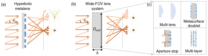
Figure 1: Wide-FOV lens systems. (a,b) Schematics of (a) a metalens with a hyperbolic phase profile and (b) a diffraction-limited lens system with a wide FOV. The former can have subwavelength thickness and produces a diffraction-limited focal spot at normal incidence but suffers from strong aberrations at oblique incidence. The latter achieves diffraction-limited focusing over a wide range of incident angles but requires a minimal thickness $h$. (c) Examples of systems that realize wide-FOV diffraction-limited focusing: cascade of multiple lenses, metasurface doublets, use of an aperture stop, and multi-layer metasurfaces.

One way to expand the FOV is to use the phase profile of an equivalent spherical lens [12] or a quadratic phase profile [19, 20, 21], which reduce off-axis aberrations. However, doing so introduces spherical aberration and defocus aberration, with a reduced effective aperture size, axial elongation, and a low Strehl ratio [12, 21, 22], so the focus is no longer diffraction-limited.

To achieve wide FOV with diffraction-limited focusing, one can use metasurface doublets [23, 24, 25, 26, 27, 28, 29, 30] or triplets [31] analogous to conventional multi-lens systems, add an aperture stop so incident light from different angles reach different regions of the metasurface [32, 33, 34, 35, 36, 37], or use inverse-designed multi-layer structures [38, 39]; these approaches are schematically illustrated in Fig. 1(b,c). Notably, all of these approaches involve a much thicker system where the overall thickness (e.g., separation between the aperture stop and the metasurface) plays a critical role. Meanwhile, miniaturization is an important consideration and motivation for metalenses. This points to the scientifically and technologically important questions: is there a fundamental trade-off between the FOV and the thickness of a metalens system, or lenses in general? If so, what is the minimal thickness allowed by physical laws?

Light propagating through disordered media exhibits an angular correlation called “memory effect” [40, 41, 42, 43, 44]: when the incident angle tilts, the transmitted wavefront stays invariant and tilts by the same amount if the input momentum tilt is smaller than roughly one over the medium thickness. Weakly scattering media like a diffuser exhibit a longer memory effect range [45], and thin layers like a metasurface also have a long memory effects range [46]. With angle-multiplexed volume holograms, it was found that a thicker hologram material is needed to store more pages of information at different angles [47, 48]. These phenomena suggest there may be an intrinsic relation between angular diversity and thickness in multi-channel systems including but not limited to lenses.

Bounds for metasurfaces can provide valuable physical insights and guidance for future designs. Shrestha et al. [49] and Presutti et al. [50] related the maximal operational bandwidth of achromatic metalenses to the numerical aperture (NA), lens diameter, and thickness, which was generalized to wide-FOV operation by Shastri et al. [51] and diffractive lenses by Engelberg et al. [52]. Shastri et al. investigated the relation between absorber efficiency and its omnidirectionality [53], Gigli et al. analyzed the limitations of Huygens’ metasurfaces due to nonlocal interactions [54], Chung et al. determined the upper bounds on the efficiencies of unit-cell-based high-NA metalenses [55], Yang et al. quantified the relation between optical performance and design parameters for aperture-stop-based metalenses [37], and Martins et al. studied the trade-off between the resolution and FOV for doublet-based metalenses [30]. Each of these studies concerns one specific type of design. The power-concentration bound of Zhang et al [56] and the multi-functional bound of Shim et al [57] are more general, though they bound the performance rather than the device footprint. However, the relationship between thickness and angular diversity remains unknown.

In this work, we establish such relationship and apply it to wide-FOV metalenses. Given any desired angle-dependent response, we can write down its transmission matrix, measure its degree of nonlocality (as encapsulated in the lateral spreading of incident waves encoded in the transmission matrix), from which we determine the minimal device thickness. This is a new approach for establishing bounds, applicable across different designs including single-layer metasurfaces, cascaded metasurfaces, diffractive lenses, bulk metamaterials, thick volumetric structures, etc.

I Thickness bound via transmission matrix

The multi-channel transport through any linear system can be described by a transmission matrix. Consider monochromatic wave at angular frequency $\omega=2\pi c/\lambda$. The incoming wavefront can be written as a superposition of propagating waves at different angles and polarizations, as

$${\bf E}_{\rm in}({\bm{\rho}},z=0)=\sum_{a=1}^{N_{\rm in}}v_{a}\hat{e}_{a}e^{i{\bf k}_{\parallel}^{a}\cdot{\bm{\rho}}}w_{\rm in}(\bm{\rho}),$$ (2)

where ${\bm{\rho}}=(x,y)$ is the transverse coordinate; $\hat{e}_{a}$ and ${\bf k}_{\parallel}^{a}=(k_{x}^{a},k_{y}^{a})$ are the polarization state and the transverse wave number (momentum) of the $a$-th plane-wave input with amplitude $v_{a}$; $z=0$ is the front surface of the lens, and $w_{\rm in}(\bm{\rho})=1$ for $|\bm{\rho}|<D_{\rm in}/2$ (zero otherwise) is a window function that describes an aperture that blocks incident light beyond entrance diameter $D_{\rm in}$. The wave number ${\bf k}_{\parallel}^{a}$ is restricted to propagating waves within the angular FOV, with $|{\bf k}_{\parallel}^{a}|<(\omega/c)\sin({\rm FOV/2})$. Since the input is band-limited in space due to the entrance aperture, a discrete sampling of ${\bf k}_{\parallel}^{a}$ with $2\pi/D_{\rm in}$ spacing at the Nyquist rate [58] is sufficient. Therefore, the number $N_{\rm in}$ of “input channels” is finite [59], and the incident wavefront is parameterized by a column vector ${\bm{v}}=[v_{1},\cdots,v_{N_{\rm in}}]^{\rm T}$. Similarly, the propagating part of the transmitted wave is a superposition of $N_{\rm out}$ output channels at different angles and polarizations,

$${\bf E}_{\rm t}({\bm{\rho}},z=h)=\sum_{b=1}^{N_{\rm out}}u_{b}\hat{e}_{b}e^{i{\bf k}_{\parallel}^{b}\cdot{\bm{\rho}}}w_{\rm out}(\bm{\rho}),$$ (3)

where $h$ is the thickness of the lens system, and the window function $w_{\rm out}(\bm{\rho})=1$ for $|\bm{\rho}|<D_{\rm out}/2$ blocks transmitted light beyond an output aperture with diameter $D_{\rm out}$. The transmitted wavefront is parameterized by column vector ${\bm{u}}=[u_{1},\cdots,u_{N_{\rm out}}]^{\rm T}$. Normalization prefactors are ignored in Eqs. (2)–(3) for simplicity.

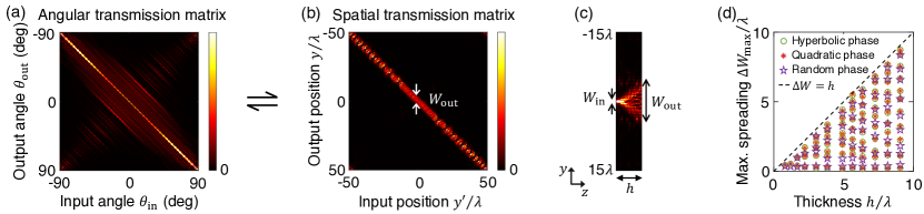
Figure 2: Transmission matrix and its relation to nonlocality and device thickness $h$. (a,b) The same transmission matrix in angular basis $|t(k_{y},k_{y}^{\prime})|^{2}$ and in spatial basis $|t(y,y^{\prime})|^{2}$, for a hyperbolic metalens with diameter $D=100\lambda$, NA = 0.45, thickness $h=4.2\lambda$, index contrast = 0.4, without a substrate ($n_{\rm in}=1$). The axes in (a) are linearly spaced in $k_{y}=(\omega/c)\sin{\theta_{\rm out}}$ and $k_{y}^{\prime}=(\omega/c)\sin{\theta_{\rm in}}$. (c) Intensity profile inside the metasurface for a localized input at $y^{\prime}=0$, corresponding to the middle column of the spatial transmission matrix. The lateral spreading $\Delta W=W_{\rm out}-W_{\rm in}$ quantifies the degree of nonlocality. (d) Maximal lateral spreading $\Delta W_{\rm max}\equiv\max_{y^{\prime}}\Delta W(y^{\prime})$ computed from $t(y,y^{\prime})$, for random metasurfaces and standard metasurfaces with varying parameters and thicknesses. The data reveal an empirical inequality $\Delta W_{\rm max}<h$, which places a lower bound on the thickness of a device that realizes the corresponding transmission matrix.

The input and the output must be related through a linear transformation, so we can write

$$u_{b}=\sum_{a=1}^{N_{\rm in}}t_{ba}v_{a},$$ (4)

or ${\bm{u}}={\bf t}{\bm{v}}$, where ${\bf t}$ is the transmission matrix [60, 61, 62]. The transmission matrix describes the exact wave transport through any linear system, regardless of the complexity of the structure and its material compositions.

For simplicity, in the examples below we consider the transverse magnetic (TM) waves of 2D systems where we only need to consider the $\hat{x}$ polarization ${\bf E}=E_{x}(y,z)\hat{x}$, with the transverse coordinate $\rho=y$ and the transverse momentum $k_{y}$ both being scalars. We compute the transmission matrix with full-wave simulations using the recently proposed augmented partial factorization method [22] implemented in the open-source software MESTI [63]. Figure 2(a) shows the squared amplitude of the transmission matrix for a 2D metalens designed to exhibit the hyperbolic phase profile in Eq. (1) at normal incidence. We informally express such transmission matrix in angular basis as $t(k_{y},k_{y}^{\prime})$ where $k_{y}^{\prime}=k_{y}^{a}=(\omega/c)\sin\theta_{\rm in}$ is the transverse momentum of the input and $k_{y}=k_{y}^{b}=(\omega/c)\sin\theta_{\rm out}$ is that of the output.

Each windowed plane-wave input or output is itself a superposition of spatially-localized waves, so we can convert the transmission matrix from the angular basis to a spatial basis with no change in its information content. Informally, such a change of basis is described by a Fourier transform $F$ on the input side and an inverse Fourier transform $F^{-1}$ on the output side [64], as

$$t(y,y^{\prime})=F^{-1}t(k_{y},k_{y}^{\prime})F.$$ (5)

A formal derivation is provided in the Supplementary Materials. Intuitively, $t(y,y^{\prime})$ gives the output at position $y$ given a localized incident wave focused at $y^{\prime}$; it has also been called the “discrete-space impulse response” [65]. Its off-diagonal elements capture nonlocal couplings between different elements of a metasurface, which are commonly ignored in conventional metasurface designs but play a critical role for angular diversity. Figure 2(b) shows the transmission matrix of Fig. 2(a) in spatial basis.

The spatial transmission matrix $t(y,y^{\prime})$ provides a measure of the nonlocality and an intuitive link to the system thickness $h$. It is expected that given a thicker device, incident light at $z=0$ can potentially spread more laterally when it reaches the other side at $z=h$. The extent of such a lateral spreading $\Delta W$ is the difference between the width of the output and that of the input,

$$\Delta W(y^{\prime})=W_{\rm out}(y^{\prime})-W_{\rm in},$$ (6)

as indicated in Fig. 2(c) on a numerically computed intensity profile with a localized incident wave. Such a lateral spreading $\Delta W$ quantifies the strength of nonlocal couplings. The output width $W_{\rm out}$ is also the vertical width of the near-diagonal elements of the spatial transmission matrix $t(y,y^{\prime})$, as indicated in Fig. 2(b).

To quantify the transverse widths, we use the inverse participation ratio (IPR) [66], with

$$W_{\rm out}(y^{\prime})=\frac{\left[\int\left|t(y,y^{\prime})\right|^{2}dy\right]^{2}}{\int\left|t(y,y^{\prime})\right|^{4}dy}.$$ (7)

For rectangular functions, the IPR equals the width of the function. The width of the input is similarly defined: in the spatial basis, each input consists of plane waves with momenta $|k_{y}^{\prime}|<(\omega/c)\sin({\rm FOV/2})$ that make up a sinc profile in space, whose IPR is $W_{\rm in}=3\lambda/[4\sin({\rm FOV/2})]$.

The nonlocal lateral spreading $\Delta W(y^{\prime})$ depends on the location $y^{\prime}$ of illumination. Since we want to relate lateral spreading to the device footprint which is typically measured by the thickness at its thickest part, below we will consider the maximal lateral spreading across the surface,

$$\Delta W_{\rm max}\equiv\max_{y^{\prime}}\Delta W(y^{\prime}).$$ (8)

Figure 2(d) shows the maximal spreading $\Delta W_{\rm max}$ as a function of thickness $h$, calculated from full-wave simulations using MESTI [63]. Here we consider metasurfaces designed to have the hyperbolic phase profile of Eq. (1) at normal incidence, metasurfaces with a quadratic phase profile [19, 20, 21] at normal incidence, and metasurfaces with random phase profiles. These data points cover NA from 0.1 to 0.9, index contrasts from 0.1 to 2, using diameter $D_{\rm out}=100\lambda$, with the full FOV $=180^{\circ}$. From these data, we observe an empirical inequality

$$\Delta W_{\rm max}<h,$$ (9)

as intuitively expected. This relation provides a quantitative link between the angle-dependent response of a system and its thickness.

Note that while higher index contrasts allow a $2\pi$ phase shift to be realized with thinner metasurfaces, such higher index contrasts do not lower the minimum thickness governed by Eq. (9). The systems considered in Fig. 2(d) have no substrate and use the full FOV; Figures S1–S2 in the Supplementary Materials further show that Eq. (9) also holds for metasurfaces sitting on a substrate or when a reduced FOV is considered. In 2D, the ratio between minimal thickness and our definition of the lateral spreading happens to be roughly 1, independent of index contrast and substrate index; we expect a similar relation in 3D, likely with a slightly different ratio.

We emphasize that even though Eq. (9) follows intuition and is found to be valid across a wide range of systems considered above, it remains empirical. In particular, in the presence of guided resonances [67, 68], it is possible for the incident wave from free space to be partially converted to a guided wave and then radiate out to the free space after some in-plane propagation, enabling the lateral spreading $\Delta W$ to exceed the thickness $h$; this is likely the case with resonance-based space-squeezing systems [69, 70, 71]. Indeed, we have found that Eq. (9) may be violated within a narrow angular range near that of a guided resonance. It is possible to extend the angular range by stacking multiple resonances [71] or by using guided resonances on a flat band [72, 73], but doing so restricts the degrees of freedom for further designs. In the following, we assume Eq. (9) is valid, which implicitly excludes broad-angle resonant effects.

Given the angle-dependent response of a system described by $t(k_{y},k_{y}^{\prime})$, Eqs. (5)–(9) quantify its degree of nonlocality and the minimal thickness such a system must have. This formalism applies to different nonlocal systems. Below, we use this formalism to establish a thickness bound for wide-FOV lenses.

II Thickness bound for wide-FOV lenses

II.1 Transmission matrix of an ideal wide-FOV lens

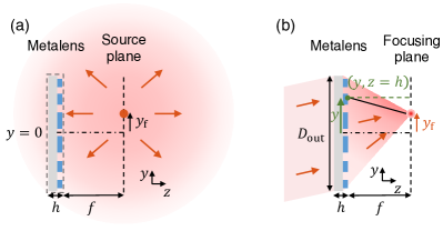
Figure 3: Schematics for determining the field transmitted through an ideal metalens. (a) Outgoing field from a point source located at the focal spot $(y=y_{\rm f},z=h+f)$. (b) To ideally focus light to such focal spot, the transmitted field across the back aperture $D_{\rm out}$ should be proportional to the complex conjugation of the radiated field in (a), given by the distance $r=\sqrt{f^{2}+(y-y_{\rm f})^{2}}$ between a point $(y,h)$ on the back of the metalens to the focal spot $(y_{\rm f},h+f)$.

To ideally focus a windowed (within $|y^{\prime}|<D_{\rm in}/2$) plane wave $E_{x}^{a}(y^{\prime},z=0)=E_{0}e^{ik_{y}^{\prime}y^{\prime}}$ incident from angle $\theta_{\rm in}$ to point ${\bf r}_{\rm f}(\theta_{\rm in})=(y=y_{\rm f}(\theta_{\rm in}),z=h+f)$ on the focal plane, the field on the back surface of a metalens should be proportional to the conjugation of the field radiated from a point source at the focal spot to the back surface, as illustrated in Fig. 3. Here we consider such ideal transmitted field across the entire back aperture of the lens within $|y|<D_{\rm out}/2$, independent of the incident angle [74]. The radiated field from a point source in 2D is proportional to $e^{ikr}/\sqrt{r}$, and the distance is $r=\sqrt{f^{2}+(y-y_{f})^{2}}$, so the ideal field on the back surface of a metalens is

$$E_{x}^{a}(y,z=h)=\begin{cases}A(\theta_{\rm in})\frac{e^{i\phi_{\rm out}^{\rm ideal}(y,\theta_{\rm in})}}{[f^{2}+(y-y_{\rm f})^{2}]^{{1}/{4}}}&\text{for }|y|<\frac{D_{\rm out}}{2}\\ 0&\text{otherwise}\end{cases},$$ (10)

where $A(\theta_{\rm in})$ is a constant amplitude, and the ideal phase distribution on the back of the metalens is [17, 9, 33]

$$\phi_{\rm out}^{\rm ideal}(y,\theta_{\rm in})=\psi(\theta_{\rm in})-\frac{2\pi}{\lambda}\sqrt{f^{2}+\left[y-y_{\rm f}(\theta_{\rm in})\right]^{2}}.$$ (11)

A global phase does not affect focusing, so we include a spatially-constant (but can be angle-dependent) phase function $\psi(\theta_{\rm in})$. For the focal spot position, we consider $y_{\rm f}(\theta_{\rm in})=f\tan\theta_{\rm in}$, such that the chief ray going through the lens center remains straight. A lens system that realizes this angle-dependent phase shift profile $\Delta\phi_{\rm ideal}(y,\theta_{\rm in})=\phi_{\rm out}^{\rm ideal}(y,\theta_{\rm in})-\phi_{\rm in}(y,\theta_{\rm in})$ within the desired $|\theta_{\rm in}|<{\rm FOV}/2$ will achieve diffraction-limited focusing with no aberration, where $\phi_{\rm in}(y,\theta_{\rm in})=(\omega/c)\sin{\theta_{\rm in}}y$ is the phase profile of the incident light.

We project the ideal output field in Eq. (10) onto a set of flux-orthogonal windowed plane-wave basis to get the angular transmission matrix $t(k_{y},k_{y}^{\prime})$, as

$$t_{ba}=\sqrt{\frac{k_{z}^{b}}{D_{\rm out}}}\int_{-\frac{D_{\rm out}}{2}}^{\frac{D_{\rm out}}{2}}E_{x}^{a}(y,z=h)e^{-ik_{y}^{b}y}dy,$$ (12)

where $k_{y}^{a}=a(2\pi/D_{\rm in})$ with $a\in\mathbb{Z}$ and $|k_{y}^{a}|<(\omega/c)\sin{(\rm FOV/2)}$, $k_{y}^{b}=b(2\pi/D_{\rm out})$ with $b\in\mathbb{Z}$ and $|k_{y}^{b}|<\omega/c$, and $(k_{y}^{a})^{2}+(k_{z}^{a})^{2}=(k_{y}^{b})^{2}+(k_{z}^{b})^{2}=(\omega/c)^{2}$. The spatial transmission matrix $t(y,y^{\prime})$ is then given by

$$t(y,y^{\prime})=\frac{1}{\sqrt{D_{\rm in}D_{\rm out}}}\sum_{b}\sum_{a}\sqrt{\frac{k_{z}^{a}}{k_{z}^{b}}}e^{ik_{y}^{b}y}t_{ba}e^{-ik_{y}^{a}y^{\prime}},$$ (13)

where $|y|<D_{\rm out}/2$ and $|y^{\prime}|<D_{\rm in}/2$. Detailed derivations and implementations of Eqs. (12)–(13) are given in Supplementary Sec. 2. From $t(y,y^{\prime})$, we obtain the lateral spreading $\Delta W(y^{\prime})$.

II.2 Thickness bound

Figure 4(a–c) plots $\Delta\phi_{\rm ideal}(y,\theta_{\rm in})$, the corresponding transmission matrix in spatial basis, and $\Delta W(y^{\prime})$ for a lens with output diameter $D_{\rm out}=400\lambda$, ${\rm NA}=\sin(\arctan(D_{\rm out}/(2f)))=0.45$ [75], ${\rm FOV}=80^{\circ}$. Here, the global phase $\psi(\theta_{\rm in})=\frac{2\pi}{\lambda}\sqrt{f^{2}+y_{\rm f}(\theta_{\rm in})^{2}}$ is chosen such that $\Delta\phi_{\rm ideal}(y=0,\theta_{\rm in})=0$. Note that unlike in Fig. 2(b), here $\Delta W(y^{\prime})$ depends strongly on the position $y^{\prime}$. An input focused at $y^{\prime}=0$ is a superposition of plane waves with different angles that constructively interfere at $y^{\prime}=0$, and since the phase shift $\Delta\phi_{\rm ideal}(y=0,\theta_{\rm in})=0$ is angle-independent there, the transmitted plane waves at different angles still interfere constructively at the output $y=0$, with no lateral spreading, so $\Delta W(y^{\prime}=0)\approx 0$. This is analogous to a transform-limited pulse (where its phase is aligned across different frequencies to yield the smallest possible pulse duration) propagating through a dispersion-free medium such that the outgoing pulse is still transform limited with no stretching, but applied to the space-angle Fourier pair instead of the time-frequency Fourier pair. However, away from the lens center, the phase shift $\Delta\phi_{\rm ideal}(y\neq 0,\theta_{\rm in})$ exhibits strong angle dependence as shown in Fig. 4(a), resulting in significant lateral spreading as shown in Fig. 4(b–c); this is analogous to pulses that propagate through a medium with strong dispersion and get significantly stretched.

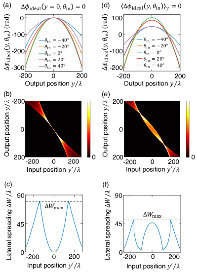
Figure 4: Angle-dependent phase shift and lateral spreading of an ideal large-FOV lens. (a–c) The incident-angle-dependent phase-shift profiles, spatial transmission matrix $\left|t(y,y^{\prime})\right|^{2}$, and lateral spreading $\Delta W(y^{\prime})$ respectively for an ideal large-FOV lens with the global phase $\psi(\theta_{\rm in})$ chosen such that $\Delta\phi_{\rm ideal}(y=0,\theta_{\rm in})=0$; this choice minimizes the angle dependence of the phase shift at $y=0$, which minimizes $\Delta W(y^{\prime}=0)$. (d–f) Corresponding plots with $\psi(\theta_{\rm in})=\psi_{0}(\theta_{\rm in})$ in Eq. (15), chosen such that $\langle\Delta\phi_{\rm ideal}(y,\theta_{\rm in})\rangle_{y}=0$ which minimizes $\Delta W_{\rm max}$ and therefore minimizes the thickness bound. Lens parameters: diameter $D_{\rm out}=400\lambda$, ${\rm NA}=0.45$, ${\rm FOV}=80^{\circ}$, with $y_{\rm f}(\theta_{\rm in})=f\tan\theta_{\rm in}$.

In the above example, $\Delta W_{\rm max}\equiv\max_{y^{\prime}}\Delta W(y^{\prime})\approx 80\lambda$. Through Eq. (9), we can then conclude that such a lens must be at least $80\lambda$ thick, regardless of how the lens is designed. This $80\lambda$ is the axial distance light must propagate in order to accumulate the desired angle-dependent phase shift and the associated lateral spreading. Recall that $\Delta W$ is also a measure of nonlocality, so the unavoidable lateral spreading here indicates that aberration-free wide-FOV lenses must be nonlocal.

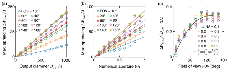
Figure 5: Dependence of the optimized maximal lateral spreading $\Delta W_{\rm max}$ on the parameters of an aberration-free wide-FOV lens. (a) $\Delta W_{\rm max}$ as a function of the output diameter $D_{\rm out}$ when ${\rm NA}=0.7$. (b) $\Delta W_{\rm max}$ as a function of the numerical aperture NA when $D_{\rm out}=300\lambda$. Symbols are the maximal spreading of such lenses, and solid lines are linear fits. (c) $\Delta W_{\rm max}/(D_{\rm out}\cdot{\rm NA})$ as a function of the FOV. Black solid line is Eq. (16).

This example uses one particular global phase function $\psi(\theta_{\rm in})=\frac{2\pi}{\lambda}\sqrt{f^{2}+y_{\rm f}(\theta_{\rm in})^{2}}$. Different $\psi(\theta_{\rm in})$ lead to different phase shifts $\Delta\phi_{\rm ideal}(y,\theta_{\rm in})=\phi_{\rm out}^{\rm ideal}(y,\theta_{\rm in})-\phi_{\rm in}(y,\theta_{\rm in})$, with different $\Delta W_{\rm max}$ and different minimal thickness. Since $\psi(\theta_{\rm in})$ does not affect the focusing quality, we can further lower the thickness bound by optimizing over $\psi(\theta_{\rm in})$ as follows.

II.3 Minimization of maximal spreading

To minimize $\Delta W_{\rm max}$ and the resulting thickness bound, we search for the function $\psi(\theta_{\rm in})$ that minimizes the maximal phase-shift difference among all possible pairs of incident angles across the whole surface,

$$\mathop{{\rm argmin}}\limits_{\psi(\theta_{\rm in})}\ \max_{y,\theta_{\rm in}^{i},\theta_{\rm in}^{j}}|\Delta\phi_{\rm ideal}(y,\theta_{\rm in}^{i};\psi)-\Delta\phi_{\rm ideal}(y,\theta_{\rm in}^{j};\psi)|^{2},$$ (14)

where $|y|<D_{\rm out}/2$ and $|\theta_{\rm in}^{i,j}|<{\rm FOV}/2$.

A sensible choice is $\psi(\theta_{\rm in})=\psi_{0}(\theta_{\rm in})$ with

$$\psi_{0}(\theta_{\rm in})=\frac{2\pi}{\lambda}\left\langle\sqrt{f^{2}+\left[y-y_{\rm f}(\theta_{\rm in})\right]^{2}}+y\sin{\theta_{\rm in}}\right\rangle_{y}$$ (15)

where $\langle\cdots\rangle_{y}$ denotes averaging over $y$ within $|y|<D_{\rm out}/2$. With this choice, the phase profiles at different incident angles are all centered around the same $y$-averaged phase, namely $\langle\Delta\phi_{\rm ideal}(y,\theta_{\rm in})\rangle_{y}=0$ for all $\theta_{\rm in}$, so the worst-case variation with respect to $\theta_{\rm in}$ is reduced. Figure 4(d–f) shows the resulting phase profile, spatial transmission matrix, and $\Delta W(y^{\prime})$ with this $\psi=\psi_{0}$. Indeed, we observe $\Delta W_{\rm max}$ to lower from $80\lambda$ to $50\lambda$ compared to the choice of $\Delta\phi_{\rm ideal}(y=0,\theta_{\rm in})=0$ in Fig. 4(c).

Eq. (14) is a convex problem [76], so its global minimum can be found with established algorithms. We use the CVX package [77, 78] to perform this convex optimization. Section 3 and Fig. S5 of Supplementary Materials show that the $\psi_{0}(\theta_{\rm in})$ in Eq. (15) is very close to the global optimum of Eq. (14), and the two give almost identical $\Delta W_{\rm max}$. Therefore, in the following we adopt the $\psi_{0}(\theta_{\rm in})$ in Eq. (15) to obtain the smallest-possible thickness bound.

One can potentially also vary the focal spot position $y_{\rm f}(\theta_{\rm in})$ to further minimize $\Delta W_{\rm max}$, since image distortions can be corrected by software. After optimizing over $y_{\rm f}$, we find that $y_{\rm f}(\theta_{\rm in})=f\tan{\theta_{\rm in}}$ already provides close-to-minimal $\Delta W_{\rm max}$.

II.4 Dependence on lens parameters

The above procedure can be applied to any wide-FOV lens. For example, we now know that the lens considered in Figure 4 must be at least $50\lambda$ thick regardless of its design. It is helpful to also know how such a minimal thickness depends on the lens parameters, so we carry out a systematic study here.

Supplementary Video 1 shows how the ideal transmission matrix in both bases evolve as the FOV increases. While increasing the FOV only adds more columns to the angular transmission matrix, doing so increases the variation of the phase shift with respect to the incident angle (i.e., increases the angular diversity), which changes the spatial transmission matrix and increases the lateral spreading (i.e., increases nonlocality). We also observe that the output profiles in $|t(y,y^{\prime})|^{2}$ develop two strong peaks at the edges as the FOV increases. The IPR in Eq. (7) is better suited for functions that are unimodal or close to rectangular. Therefore, when FOV $\geq 100^{\circ}$, we use the full width at half maximum (FWHM) instead to quantify $W_{\rm out}$; Figure S7 of the Supplementary Materials shows that the FWHM equals IPR for small FOV but is a better measure of the output width for large FOV.

Table 1: Metalenses with diffraction-limited focusing over a wide FOV^a

	Method	Exp./ Sim.	Output diameter $D_{\rm out}$($D_{\rm out}^{\rm eff}$)	Numerical aperture	FOV (air)	Strehl ratio	Total thickness	Thickness bound
Arbabi et al. [23]	Doublet	3D Exp.	(800 $\upmu$m)	0.49	$60^{\circ}$	$\gtrsim 0.9$	1 mm	92 $\upmu$m
Groever et al. [24]	Doublet	3D Exp.	(313 $\upmu$m)	0.44	$50^{\circ}$	$\gtrsim 0.8$	500 $\upmu$m	30 $\upmu$m
He et al. [25]	Doublet	3D Sim.	(400 $\upmu$m)	0.47	$60^{\circ}$	-	500 $\upmu$m	44 $\upmu$m
Li et al. [26]	Doublet	3D Sim.	(20 $\upmu$m)	0.45	$50^{\circ}$	$\gtrsim 0.5$	31.2 $\upmu$m	1.8 $\upmu$m
Tang et al. [27]	Doublet	3D Sim.	(30 $\upmu$m)	0.35	$40^{\circ}$	-	21.2 $\upmu$m	1.8 $\upmu$m
Kim et al. [28]	Doublet	3D Sim.	(300 $\upmu$m)	0.38	$60^{\circ}$	-	500 $\upmu$m	27 $\upmu$m
Huang et al. [29]	Doublet	3D Sim.	(5 $\upmu$m)	0.60	$60^{\circ}$	-	6.6 $\upmu$m	0.7 $\upmu$m
Engelberg et al. [32]	Aperture	3D Exp.	(1.35 mm)	0.20	$30^{\circ}$	-	3.36 mm	0.03 mm
Shalaginov et al. [33] Shalaginov et al. [33]	Aperture Aperture	3D Exp. 3D Sim.	(1 mm) (1 mm)	0.24 0.20	$\sim 180^{\circ}$ $\sim 180^{\circ}$	$\gtrsim 0.8$ $\gtrsim 0.8$	2 mm 3.9 mm	0.08 mm 0.07 mm
Fan et al. [34]	Aperture	3D Sim.	(20 $\upmu$m)	0.25	$170^{\circ}$	$\gtrsim 0.8$	$38.6\ \upmu$m	1.7 $\upmu$m
Zhang et al. [35]	Aperture	3D Exp.	(1 mm)	0.11	$\sim 180^{\circ}$	-	5.44 mm	0.04 mm
Yang et al. [36]	Aperture	3D Sim.	(100 $\upmu$m)	0.18	$\sim 180^{\circ}$	$\sim 0.64$	200 $\upmu$m	6 $\upmu$m
Lin et al. [38]	Multi-layer	2D Sim.	$23\lambda$	0.35	$40^{\circ}$	-	$1.5\lambda$	$1.4\lambda$
Lin et al. [39] Lin et al. [39] Lin et al. [39]	Multi-layer Multi-layer Multi-layer	2D Sim. 2D Sim. 3D Sim.	$50\lambda$ $125\lambda$ $50\lambda$	0.24 0.70 0.12	$60^{\circ}$ $80^{\circ}$ $16^{\circ}$	$\gtrsim 0.8$ $\gtrsim 0.8$ $\gtrsim 0.8$	$12\lambda$ $24\lambda$ $12\lambda$	$2.8\lambda$ $25\lambda$ $0.4\lambda$

• We note that the thickness bound here is directly from Eq. (17), which is an approximate expression and is obtained for 2D systems but suffices as an estimation. Refs. [23, 24, 25, 26, 27, 28, 29, 32, 33, 34, 35, 36] adopt a telecentric configuration where each incident angle fills an effective diameter $D_{\rm out}^{\rm eff}$ within the output aperture, which we use in place of $D_{\rm out}$ when evaluating their thickness bounds. Some works also correct the chromatic aberration: at 473 nm and 532 nm in Ref. [27], at 445 nm, 532 nm and 660 nm in Ref. [28], from 470 nm to 650 nm in Ref. [29], and from 1 to 1.2 $\upmu$m in Ref. [36]. Ref. [38] achieves diffraction-limited focusing for 7 angles within the FOV. Ref. [39] achieves diffraction-limited focusing for 19, 7 and 9 angles within the FOV and also corrects the chromatic aberration for 10, 4, and 5 frequencies within a 23% spectral bandwidth from up to down.

Next, we quantify the dependence on all lens parameters. Figure 5 plots the optimized maximal lateral spreading $\Delta W_{\rm max}$ as a function of the output diameter $D_{\rm out}$, NA and the FOV. As shown in Fig. 5(a), $\Delta W_{\rm max}$ grows linearly with $D_{\rm out}$ for different FOV. Figure 5(b) further shows that $\Delta W_{\rm max}$ also grows approximately linearly with the numerical aperture NA. Figure 5(a,b) fix ${\rm NA}=0.7$ and $D_{\rm out}=300\lambda$ respectively, while similar dependencies are observed for other lens parameters (Figs. S8–9 of Supplementary Materials). Dividing by $D_{\rm out}$ and NA, we obtain how $\Delta W_{\rm max}$ depends on the FOV, shown in Fig. 5(c). The angular range is governed by $\sin({\rm FOV}/2)$, but the functional dependence of $\Delta W_{\rm max}$ on the FOV is not simply $\sin({\rm FOV}/2)$; empirically, we find the function $\frac{1}{3}\sin(\frac{\pi}{2}\sin\frac{\rm FOV}{2})$ to provide a reasonable fit for the FOV dependence. These dependencies can be summarized as

$$\Delta W_{\rm max}\approx(\frac{1}{3}{\rm NA})D_{\rm out}\sin\left(\frac{\pi}{2}\sin\frac{\rm FOV}{2}\right).$$ (16)

Eq. (9) and Eq. (16) then tell us approximately how the thickness bound varies with the lens parameters,

$$h\gtrsim(\frac{1}{3}{\rm NA})D_{\rm out}\sin\left(\frac{\pi}{2}\sin\frac{\rm FOV}{2}\right).$$ (17)

This result makes intuitive sense, since increasing the NA, aperture size, and/or FOV will all lead to an increased phase-shift variation, which leads to the increased minimal thickness.

Any aberration-free wide-FOV lens system must have a transmission matrix described in Sec. II.1, so the above bound applies to any such system regardless of how the system is designed (barring unlikely broad-angle resonant effects). This result shows that to achieve large FOV with a wide output aperture, a single layer of subwavelength-thick metasurface is fundamentally not sufficient. Meanwhile, it also reveals room to make existing designs more compact, as we discuss below.

While the results above are obtained for 2D systems, we expect qualitatively similar results in 3D (possibly only with a slightly different prefactor) since the relation between angular diversity and lateral spreading and the relation between lateral spreading and thickness are both generic. Note that we use FOV to denote the range of incident angles from air. Equation (17) continues to hold in the presence of substrates, with the Snell’s law $\sin\frac{\rm FOV}{2}=n_{\rm in}\sin\frac{\rm FOV_{in}}{2}$ for ${\rm FOV}_{\rm in}$ in a substrate with refractive index $n_{\rm in}$, since we have shown in Fig. S1 that Eq. (9) holds in the presence of a substrate and since the ideal transmission matrix in Sec. II.1 is the same with or without a substrate.

Table 1 lists diffraction-limited wide-FOV metalens systems reported in the literature. All of them have total thickness consistent with Eq. (17). A few inverse-designed multi-layer structures [38, 39] have thickness close to the bound, suggesting that the bound is tight. Note that the second design in Ref. [39] has a slightly smaller thickness ($24\lambda$) than the bound ($25\lambda$), likely because it only optimizes for diffraction-limited focusing at a discrete set of angles. Existing metalenses based on doublets or aperture stops are substantially thicker than the bound, which is sensible since those systems have ample amount of free spaces not used for structural design.

Here we consider ideal aberration-free focusing for all incident angles within the FOV. Relaxing some of these conditions can relax the thickness bound; for example, if diffraction-limited focusing is not necessary, the quadratic phase profile [19, 20, 21] can eliminate the angle dependence of the phase profile. Meanwhile, achromatic wide-FOV lenses [31, 27, 28, 29, 39, 36] will be subject to additional constraints beyond nonlocality [51].

III Discussion

Due to the Fourier-transform duality between space and momentum, any multi-channel system with an angle-dependent response will necessarily require nonlocality and spatial spreading (exemplified in Fig. 4 and analogous to a pulse propagating through a dispersive medium under time-frequency duality), which is tied to the device thickness through Eq. (9). This relationship is not limited to wide-FOV lenses and establishes the intrinsic link between angular diversity and spatial footprint suggested in the introduction.

For example, one can readily use this approach to establish thickness bounds for other types of nonlocal metasurfaces such as retroreflectors [79] and photovoltaic concentrators [80, 81, 38, 82] where a wide angular range is also desirable. Note that concentrators are additionally subject to efficiency bounds arising from passivity and/or reciprocity [56].

These results can guide the design of future nonlocal metasurfaces, providing realistic targets for device dimensions. While multi-layer metasurfaces that reach Eq. (17) have not been experimentally realized yet, there are several realistic routes. A stacked triple-layer metalens has been reported [31]. Multi-layer structures have been realized with two-photon polymerization [83, 82, 84], or repeated deposition and patterning of 2D layers [85, 86, 87, 88]. Volumetric nanostructures may also be realized with deposition onto shrinking scaffolds [89]. Additionally, multi-level diffractive lenses can readily have thickness above 10 $\mu$m [90, 91].

Fundamental bounds like this are valuable as metasurface research evolves beyond single-layer local designs, as better control of light is achieved over wider ranges of angles, and with the continued push toward ultra-compact photonic devices. Future work can investigate designs incorporating broad-angle resonant responses. We also note that the transmission-matrix approach is versatile and can be used to establish other types of bounds beyond the device footprint.

References

- [1] Yu, N. et al. Light propagation with phase discontinuities: generalized laws of reflection and refraction. Science 334, 333–337 (2011).
- [2] Kildishev, A. V., Boltasseva, A. & Shalaev, V. M. Planar photonics with metasurfaces. Science 339, 1232009 (2013).
- [3] Yu, N. & Capasso, F. Flat optics with designer metasurfaces. Nat. Mater. 13, 139–150 (2014).
- [4] Chen, H.-T., Taylor, A. J. & Yu, N. A review of metasurfaces: physics and applications. Rep. Prog. Phy. 79, 076401 (2016).
- [5] Genevet, P., Capasso, F., Aieta, F., Khorasaninejad, M. & Devlin, R. Recent advances in planar optics: from plasmonic to dielectric metasurfaces. Optica 4, 139–152 (2017).
- [6] Hsiao, H.-H., Chu, C. H. & Tsai, D. P. Fundamentals and applications of metasurfaces. Small Methods 1, 1600064 (2017).
- [7] Kamali, S. M., Arbabi, E., Arbabi, A. & Faraon, A. A review of dielectric optical metasurfaces for wavefront control. Nanophotonics 7, 1041–1068 (2018).
- [8] Chen, W. T., Zhu, A. Y. & Capasso, F. Flat optics with dispersion-engineered metasurfaces. Nat. Rev. Mater. 5, 604–620 (2020).
- [9] Lalanne, P. & Chavel, P. Metalenses at visible wavelengths: past, present, perspectives. Laser Photonics Rev. 11, 1600295 (2017).
- [10] Khorasaninejad, M. & Capasso, F. Metalenses: Versatile multifunctional photonic components. Science 358, eaam8100 (2017).
- [11] Tseng, M. L. et al. Metalenses: advances and applications. Adv. Opt. Mater. 6, 1800554 (2018).
- [12] Liang, H. et al. High performance metalenses: numerical aperture, aberrations, chromaticity, and trade-offs. Optica 6, 1461–1470 (2019).
- [13] Kim, S.-J. et al. Dielectric metalens: properties and three-dimensional imaging applications. Sensors 21, 4584 (2021).
- [14] Hecht, E. Chapter 5.2: Lenses. In Optics, 5ed (Pearson Education Limited, 2017).
- [15] Aieta, F. et al. Aberration-free ultrathin flat lenses and axicons at telecom wavelengths based on plasmonic metasurfaces. Nano Lett. 12, 4932–4936 (2012).
- [16] Aieta, F., Genevet, P., Kats, M. & Capasso, F. Aberrations of flat lenses and aplanatic metasurfaces. Opt. Express 21, 31530–31539 (2013).
- [17] Kalvach, A. & Szabó, Z. Aberration-free flat lens design for a wide range of incident angles. J. Opt. Soc. Am. B 33, A66–A71 (2016).
- [18] Decker, M. et al. Imaging performance of polarization-insensitive metalenses. ACS Photonics 6, 1493–1499 (2019).
- [19] Pu, M., Li, X., Guo, Y., Ma, X. & Luo, X. Nanoapertures with ordered rotations: symmetry transformation and wide-angle flat lensing. Opt. Express 25, 31471–31477 (2017).
- [20] Martins, A. et al. On metalenses with arbitrarily wide field of view. ACS Photonics 7, 2073–2079 (2020).
- [21] Lassalle, E. et al. Imaging properties of large field-of-view quadratic metalenses and their applications to fingerprint detection. ACS Photonics 8, 1457–1468 (2021).
- [22] Lin, H.-C., Wang, Z. & Hsu, C. W. Full-wave solver for massively multi-channel optics using augmented partial factorization. arXiv:2205.07887 (2022).
- [23] Arbabi, A. et al. Miniature optical planar camera based on a wide-angle metasurface doublet corrected for monochromatic aberrations. Nat. Commun. 7, 13682 (2016).
- [24] Groever, B., Chen, W. T. & Capasso, F. Meta-lens doublet in the visible region. Nano Lett. 17, 4902–4907 (2017).
- [25] He, D. et al. Polarization-insensitive meta-lens doublet with large view field in the ultraviolet region. In 9th International Symposium on Advanced Optical Manufacturing and Testing Technologies: Meta-Surface-Wave and Planar Optics, 108411A (International Society for Optics and Photonics, 2019).
- [26] Li, Z. et al. Super-oscillatory metasurface doublet for sub-diffraction focusing with a large incident angle. Opt. Express 29, 9991–9999 (2021).
- [27] Tang, D., Chen, L., Liu, J. & Zhang, X. Achromatic metasurface doublet with a wide incident angle for light focusing. Opt. Express 28, 12209–12218 (2020).
- [28] Kim, C., Kim, S.-J. & Lee, B. Doublet metalens design for high numerical aperture and simultaneous correction of chromatic and monochromatic aberrations. Opt. Express 28, 18059–18076 (2020).
- [29] Huang, Z., Qin, M., Guo, X., Yang, C. & Li, S. Achromatic and wide-field metalens in the visible region. Opt. Express 29, 13542–13551 (2021).
- [30] Martins, A., Li, J., Borges, B.-H. V., Krauss, T. F. & Martins, E. R. Fundamental limits and design principles of doublet metalenses. Nanophotonics 11, 1187–1194 (2022).
- [31] Shrestha, S., Overvig, A. & Yu, N. Multi-element meta-lens systems for imaging. In 2019 Conference on Lasers and Electro-Optics (CLEO), paper FF2B.8 (2019).
- [32] Engelberg, J. et al. Near-IR wide-field-of-view Huygens metalens for outdoor imaging applications. Nanophotonics 9, 361–370 (2020).
- [33] Shalaginov, M. Y. et al. Single-element diffraction-limited fisheye metalens. Nano Lett. 20, 7429–7437 (2020).
- [34] Fan, C.-Y., Lin, C.-P. & Su, G.-D. J. Ultrawide-angle and high-efficiency metalens in hexagonal arrangement. Sci. Rep. 10, 15677 (2020).
- [35] Zhang, F. et al. Extreme-angle silicon infrared optics enabled by streamlined surfaces. Adv. Mater. 33, 2008157 (2021).
- [36] Yang, F. et al. Design of broadband and wide-field-of-view metalenses. Opt. Lett. 46, 5735–5738 (2021).
- [37] Yang, F. et al. Wide field-of-view flat lens: an analytical formalism. arXiv:2108.09295 (2021).
- [38] Lin, Z., Groever, B., Capasso, F., Rodriguez, A. W. & Lončar, M. Topology-optimized multilayered metaoptics. Phys. Rev. Appl. 9, 044030 (2018).
- [39] Lin, Z., Roques-Carmes, C., Christiansen, R. E., Soljačić, M. & Johnson, S. G. Computational inverse design for ultra-compact single-piece metalenses free of chromatic and angular aberration. Appl. Phys. Lett. 118, 041104 (2021).
- [40] Freund, I., Rosenbluh, M. & Feng, S. Memory effects in propagation of optical waves through disordered media. Phys. Rev. Lett. 61, 2328 (1988).
- [41] Berkovits, R., Kaveh, M. & Feng, S. Memory effect of waves in disordered systems: a real-space approach. Phys. Rev. B 40, 737 (1989).
- [42] Osnabrugge, G., Horstmeyer, R., Papadopoulos, I. N., Judkewitz, B. & Vellekoop, I. M. Generalized optical memory effect. Optica 4, 886–892 (2017).
- [43] Yılmaz, H. et al. Angular memory effect of transmission eigenchannels. Phys. Rev. Lett. 123, 203901 (2019).
- [44] Yılmaz, H., Kühmayer, M., Hsu, C. W., Rotter, S. & Cao, H. Customizing the angular memory effect for scattering media. Phys. Rev. X 11, 031010 (2021).
- [45] Schott, S., Bertolotti, J., Léger, J.-F., Bourdieu, L. & Gigan, S. Characterization of the angular memory effect of scattered light in biological tissues. Opt. Express 23, 13505–13516 (2015).
- [46] Jang, M. et al. Wavefront shaping with disorder-engineered metasurfaces. Nat. Photonics 12, 84–90 (2018).
- [47] Li, H.-Y. S. & Psaltis, D. Three-dimensional holographic disks. Appl. Opt. 33, 3764–3774 (1994).
- [48] Barbastathis, G. & Psaltis, D. Volume holographic multiplexing methods. In Holographic data storage, 21–62 (Springer, 2000).
- [49] Shrestha, S., Overvig, A. C., Lu, M., Stein, A. & Yu, N. Broadband achromatic dielectric metalenses. Light Sci. Appl. 7, 85 (2018).
- [50] Presutti, F. & Monticone, F. Focusing on bandwidth: achromatic metalens limits. Optica 7, 624–631 (2020).
- [51] Shastri, K. & Monticone, F. Bandwidth bounds for wide-field-of-view dispersion-engineered achromatic metalenses. arXiv:2204.09154 (2022).
- [52] Engelberg, J. & Levy, U. Achromatic flat lens performance limits. Optica 8, 834–845 (2021).
- [53] Shastri, K. & Monticone, F. Existence of a fundamental tradeoff between absorptivity and omnidirectionality in metasurfaces. In 2021 Conference on Lasers and Electro-Optics (CLEO), paper JW1A.98 (2021).
- [54] Gigli, C. et al. Fundamental limitations of Huygens’ metasurfaces for optical beam shaping. Laser Photonics Rev. 15, 2000448 (2021).
- [55] Chung, H. & Miller, O. D. High-NA achromatic metalenses by inverse design. Opt. Express 28, 6945–6965 (2020).
- [56] Zhang, H., Hsu, C. W. & Miller, O. D. Scattering concentration bounds: brightness theorems for waves. Optica 6, 1321–1327 (2019).
- [57] Shim, H., Kuang, Z., Lin, Z. & Miller, O. D. Fundamental limits to multi-functional and tunable nanophotonic response. arXiv:2112.10816 (2021).
- [58] Landau, H. Sampling, data transmission, and the Nyquist rate. Proceedings of the IEEE 55, 1701–1706 (1967).
- [59] Miller, D. A. Waves, modes, communications, and optics: a tutorial. Adv. Opt. Photonics 11, 679–825 (2019).
- [60] Popoff, S. M. et al. Measuring the transmission matrix in optics: an approach to the study and control of light propagation in disordered media. Phys. Rev. Lett. 104, 100601 (2010).
- [61] Mosk, A. P., Lagendijk, A., Lerosey, G. & Fink, M. Controlling waves in space and time for imaging and focusing in complex media. Nat. Photonics 6, 283–292 (2012).
- [62] Rotter, S. & Gigan, S. Light fields in complex media: Mesoscopic scattering meets wave control. Rev. Mod. Phys. 89, 015005 (2017).
- [63] Lin, H.-C., Wang, Z. & Hsu, C. W. MESTI. https://github.com/complexphoton/MESTI.m.
- [64] Judkewitz, B., Horstmeyer, R., Vellekoop, I. M., Papadopoulos, I. N. & Yang, C. Translation correlations in anisotropically scattering media. Nat. Phys. 11, 684–689 (2015).
- [65] Torfeh, M. & Arbabi, A. Modeling metasurfaces using discrete-space impulse response technique. ACS Photonics 7, 941–950 (2020).
- [66] Yılmaz, H., Hsu, C. W., Yamilov, A. & Cao, H. Transverse localization of transmission eigenchannels. Nat. Photonics 13, 352–358 (2019).
- [67] Fan, S. & Joannopoulos, J. D. Analysis of guided resonances in photonic crystal slabs. Phys. Rev. B 65, 235112 (2002).
- [68] Gao, X. et al. Formation mechanism of guided resonances and bound states in the continuum in photonic crystal slabs. Sci. Rep. 6, 31908 (2016).
- [69] Reshef, O. et al. An optic to replace space and its application towards ultra-thin imaging systems. Nat. Commun. 12, 3512 (2021).
- [70] Guo, C., Wang, H. & Fan, S. Squeeze free space with nonlocal flat optics. Optica 7, 1133–1138 (2020).
- [71] Chen, A. & Monticone, F. Dielectric nonlocal metasurfaces for fully solid-state ultrathin optical systems. ACS Photonics 8, 1439–1447 (2021).
- [72] Leykam, D., Andreanov, A. & Flach, S. Artificial flat band systems: from lattice models to experiments. Advances in Physics: X 3, 1473052 (2018).
- [73] Leykam, D. & Flach, S. Perspective: Photonic flatbands. APL Photonics 3, 070901 (2018).
- [74] The angular distribution of the output depends on the incident angle, so the lens is not telecentric.
- [75] We define NA based on normal incidence.
- [76] Boyd, S., Boyd, S. P. & Vandenberghe, L. Convex optimization (Cambridge university press, 2004).
- [77] Grant, M. & Boyd, S. CVX: Matlab software for disciplined convex programming, version 2.1. http://cvxr.com/cvx (2014).
- [78] Grant, M. & Boyd, S. Graph implementations for nonsmooth convex programs. In Blondel, V., Boyd, S. & Kimura, H. (eds.) Recent Advances in Learning and Control, Lecture Notes in Control and Information Sciences, 95–110 (Springer-Verlag Limited, 2008).
- [79] Arbabi, A., Arbabi, E., Horie, Y., Kamali, S. M. & Faraon, A. Planar metasurface retroreflector. Nat. Photonics 11, 415–420 (2017).
- [80] Price, J. S., Sheng, X., Meulblok, B. M., Rogers, J. A. & Giebink, N. C. Wide-angle planar microtracking for quasi-static microcell concentrating photovoltaics. Nat. Commun. 6, 6223 (2015).
- [81] Shameli, M. A. & Yousefi, L. Absorption enhancement in thin-film solar cells using an integrated metasurface lens. J. Opt. Soc. Am. B 35, 223–230 (2018).
- [82] Roques-Carmes, C. et al. Towards 3D-printed inverse-designed metaoptics. ACS Photonics 9, 43–51 (2022).
- [83] Christiansen, R. E. et al. Fullwave maxwell inverse design of axisymmetric, tunable, and multi-scale multi-wavelength metalenses. Opt. Express 28, 33854–33868 (2020).
- [84] Roberts, G., Ballew, C., Foo, I., Hon, P. & Faraon, A. Experimental demonstration of 3D inverse designed metaoptics in mid-infrared. In 2022 Conference on Lasers and Electro-Optics (CLEO), paper FW5H.2 (2022).
- [85] Sherwood-Droz, N. & Lipson, M. Scalable 3D dense integration of photonics on bulk silicon. Opt. Express 19, 17758–17765 (2011).
- [86] Zhou, Y. et al. Multilayer noninteracting dielectric metasurfaces for multiwavelength metaoptics. Nano Lett. 18, 7529–7537 (2018).
- [87] Mansouree, M. et al. Multifunctional 2.5D metastructures enabled by adjoint optimization. Optica 7, 77–84 (2020).
- [88] Camayd-Muñoz, P., Ballew, C., Roberts, G. & Faraon, A. Multifunctional volumetric meta-optics for color and polarization image sensors. Optica 7, 280–283 (2020).
- [89] Oran, D. et al. 3D nanofabrication by volumetric deposition and controlled shrinkage of patterned scaffolds. Science 362, 1281–1285 (2018).
- [90] Meem, M. et al. Broadband lightweight flat lenses for long-wave infrared imaging. Proc. Nati. Acad. Sci. U.S.A. 116, 21375–21378 (2019).
- [91] Meem, M. et al. Imaging from the visible to the long-wave infrared wavelengths via an inverse-designed flat lens. Opt. Express 29, 20715–20723 (2021).