$Sp(2N)$ Yang-Mills theories on the lattice: scale setting and topology

Abstract

We study Yang-Mills lattice theories with $Sp(N_{c})$ gauge group, with $N_{c}=2N$, for $N=1,\,\cdots,\,4$. We show that if we divide the renormalised couplings appearing in the Wilson flow by the quadratic Casimir $C_{2}(F)$ of the $Sp(N_{c})$ group, then the resulting quantities display a good agreement among all values of $N_{c}$ considered, over a finite interval in flow time. We use this scaled version of the Wilson flow as a scale-setting procedure, compute the topological susceptibility of the $Sp(N_{c})$ theories, and extrapolate the results to the continuum limit for each $N_{c}$.

I Introduction

Lattice studies of $Sp(N_{c}=2N)$ gauge theories aim at quantitatively appraising, in the strong coupling regime, what are their distinctive features in respect to theories based upon $SU(N_{c})$ gauge groups. For example, a long list of recent investigations of the $SU(2)\sim Sp(2)$ theories Hietanen:2014xca ; Detmold:2014kba ; Arthur:2016dir ; Arthur:2016ozw ; Pica:2016zst ; Lee:2017uvl ; Drach:2017btk ; Drach:2020wux ; Drach:2021uhl , and of the $Sp(2N)$ theories for $N>1$ Bennett:2017kga ; Lee:2018ztv ; Bennett:2019jzz ; Bennett:2019cxd ; Bennett:2020hqd ; Bennett:2020qtj ; Bennett:2022yfa ; AS , are motivated by their paradigm changing potential for applications in contemporary high energy physics.

Prominently, enhanced global symmetry and symmetry breaking patterns arise in $Sp(2N)$ theories in the presence of matter fields. This feature is exploited in new-physics model-building exercises such as in the minimal model in Ref. Barnard:2013zea , which combines a composite Higgs model (CHM)— in which the Higgs fields originate as pseudo-Nambu-Goldstone bosons (PNGBs) in a new strongly coupled sector Kaplan:1983fs ; Georgi:1984af ; Dugan:1984hq —with partial top compositeness Kaplan:1991dc . For recent reviews see Refs. Panico:2015jxa ; Witzel:2019jbe ; Cacciapaglia:2020kgq , and the summary tables in Refs. Ferretti:2013kya ; Ferretti:2016upr ; Cacciapaglia:2019bqz . In the different context of dark matter models emerging from strongly-coupled dynamics Hochberg:2014dra ; Hochberg:2014kqa ; Hochberg:2015vrg ; Kondo:2022lgg , $Sp(2N)$ gauge theories have also been attracting increasing interest Bernal:2017mqb ; Berlin:2018tvf ; Bernal:2019uqr ; Cai:2020njb ; Tsai:2020vpi ; Maas:2021gbf ; Zierler:2021cfa ; Kulkarni:2022bvh .

There are more general, theoretical reasons to study $Sp(2N)$ gauge theories. Pioneering studies of the pure gauge cases Holland:2003kg aimed at qualifying the role of the centre symmetry in the confinement/deconfinement transition at finite temperature. In the light of the conjectured existence of dualities between large-$N_{c}$ gauge theories and theories of gravity in higher dimension Maldacena:1997re ; Gubser:1998bc ; Witten:1998qj ; Aharony:1999ti , the appeal of $Sp(N_{c})$ theories derives from the common features that they share with $SU(N_{c})$ theories. For example, extensive studies of the spectrum of glueballs and strings confirm that universal features emerge at large $N_{c}$, common to $SU(N_{c})$, $Sp(N_{c})$, and $SO(N_{c})$ theories Lucini:2001ej ; Lucini:2004my ; Lucini:2010nv ; Lucini:2012gg ; Athenodorou:2015nba ; Lau:2017aom ; Hong:2017suj ; Yamanaka:2021xqh ; Hernandez:2020tbc ; Athenodorou:2021qvs ; Bonanno:2022yjr ; Bennett:2020hqd ; Bennett:2020qtj .

The topological susceptibility, $\chi$ (to be defined in the body of the paper), plays a central role in our understanding of QCD, for several intercorrelated reasons of historical significance. It enters the Witten-Veneziano formula Witten:1979vv ; Veneziano:1979ec for the large-$N_{c}$ behaviour of the mass of the $\eta^{\prime}$ meson, and the solution to the $U(1)_{A}$ problem. Allowing the gauge coupling to be complex, and expanding in powers of (small) $\theta$, $\chi$ appears as the coefficient at $O(\theta^{2})$ in the free energy. Indirectly, it might hence have implications for the strong-CP problem, for the physics of putative new particles such as the axion, and for the electric dipole moments of hadrons. Many interesting lattice calculations of $\chi$ exist—see Refs. Lucini:2001ej ; DelDebbio:2002xa ; Lucini:2004yh ; DelDebbio:2004ns ; Luscher:2010ik ; Panagopoulos:2011rb ; Bonati:2015sqt ; Bonanno:2020hht ; Ce:2016awn ; Bonati:2016tvi ; Alexandrou:2017hqw ; Borsanyi:2021gqg ; Cossu:2021bgn ; Athenodorou:2021qvs ; Teper:2022mmj , and Tables 1 and 2 of the review in Ref. Vicari:2008jw .

Accounting for $\chi$ might provide new insight in the role of instantons and other non-perturbative objects. A precise knowledge of $\chi$ might have unexpectedly important consequences also in the aforementioned subfield encompassing modern phenomenological applications of strongly-coupled $Sp(N_{c})$ theories—models of composite Higgs, partial top compositeness, dark matter, or even early universe physics. In general, precise calculations of $\chi$ might sharpen our understanding both of commonalities and differences between $Sp(N_{c})$ and $SU(N_{c})$ theories, starting in the Yang-Mills (pure gauge) theories.

Motivated by such considerations, and as an important step in the programme of study of $Sp(N_{c})$ lattice gauge theories conducted by our collaboration, in this paper we compute the topological susceptibility of $Sp(N_{c})$ Yang-Mills theories for $N_{c}\leq 8$. We made available preliminary results in contributions to Conference Proceedings Lucini:2021xke ; Bennett:2021mbw , but this analysis is much improved, and based on larger statistics. In a dedicated publication, we compare our results for $Sp(N_{c})$ with the $SU(N_{c})$ literature, and discuss the large-$N_{c}$ extrapolation Bennett:2022gdz .

The paper is organised as follows. In Sect. II we define the lattice theories of interest. In Sect. III we discuss how to use the gradient flow and its lattice implementation, the Wilson flow Luscher:2010iy ; Luscher:2013vga , as a scale setting procedure, and define the topological charge and susceptibility. Sect. IV is the main body of the paper, in which we present our numerical results. We conclude with the summary in Sect. V. We relegate some useful details to Appendix A.

II $Sp(2N)$ Yang-Mills theories

We define the continuum $Sp(2N)$ gauge theories, in $4$-dimensional Euclidean space, in terms of the action

$$S_{\mathrm{YM}}\equiv-\frac{1}{2g_{0}^{2}}\int\mathrm{d}^{4}x\,{\rm Tr\,}F_{\mu\nu}F^{\mu\nu}~{},$$ (1)

where $g_{0}$ is the gauge coupling, $F_{\mu\nu}\equiv\sum_{A}F_{\mu\nu}^{A}\tau^{A}$, with

$$F_{\mu\nu}^{A}=\partial_{\mu}A_{\nu}^{A}-\partial_{\nu}A_{\mu}^{A}+f^{ABC}A_{\mu}^{B}A_{\nu}^{C}\,,$$ (2)

and the trace is over the color index on the fundamental representation, while $A=1,\cdots,N(2N+1)$. The Hermitian matrices $\tau^{A}\in\mathbb{C}^{2N\times 2N}$ are the generators of the algebra associated to the Lie group $Sp(2N)$ in the fundamental representation. They satisfy the relations

$$\left[\tau^{A},\,\tau^{B}\right]=\dot{\imath}f^{ABC}\tau^{C}\,,$$ (3)

and are normalised according to ${\rm Tr\,}\left(\tau^{A}\tau^{B}\right)=\frac{1}{2}\delta^{AB}$.

The configuration space of this theory can be partitioned into sectors, characterised by the value of the topological charge $Q$, defined as follows:

$$Q\equiv\int\mathrm{d}^{4}x~{}q(x)\,,$$ (4)

where

$$q(x)\equiv\frac{1}{32\pi^{2}}\epsilon^{\mu\nu\rho\sigma}\,\mathrm{Tr}~{}F_{\mu\nu}(x)F_{\rho\sigma}(x)\,.$$ (5)

The topological susceptibility, $\chi$, is defined as

$$\chi\equiv\int\mathrm{d}^{4}x~{}\langle q(x)q(0)\rangle.$$ (6)

The possible values of $Q$ belong to the third homotopy group of the gauge group. Since $Sp(2N)$ is compact, connected and simple, one finds that

$$\pi_{3}(Sp(2N))=\mathbb{Z}\,,$$ (7)

as in the case of $SU(N_{c})$ gauge theories.

II.1 The lattice

A lattice regularisation of the theory defined in Eq. (1) allows to characterise quantitatively its non-perturbative features. We adopt a $4$-dimensional Euclidean hypercubic lattice $\Lambda$, with lattice spacing $a$. The sites of the lattice are denoted by their Cartesian coordinates $x=\left\{x_{\mu}\right\}$ and the links by $(x,\,\mu)$, where $\mu=0,\,\cdots,\,3$ and $x_{\mu}=n_{\mu}a$. For a lattice of length $L_{\mu}$ in the $\mu$ directions, with $n_{\mu}=0,\,\cdots,\,L_{\mu}/a-1$, the total number of sites is thus $V_{4}/a^{4}=L_{0}L_{1}L_{2}L_{3}/a^{4}$. The lattices used in our calculations are isotropic in the four directions, $L_{\mu}=L$, and we impose periodic boundary conditions in all directions. The elementary degrees of freedom of the theory are called link variables, and defined as

$$U_{\mu}(x)\equiv\exp\left(\dot{\imath}\int_{x}^{x+\hat{\mu}}\mathrm{d}\lambda^{\mu}\tau^{A}A_{\mu}^{A}(\lambda)\right)\,,$$ (8)

where $\hat{\mu}$ is the unit vector in direction $\mu$. The link variables are $2N\times 2N$ matrices that, under the action of a gauge transformation $g(x)\in Sp(2N)$, transform as

$$U_{\mu}(x)\rightarrow g(x)U_{\mu}(x)g^{\dagger}(x+\hat{\mu})\,.$$ (9)

The trace of a path-ordered product of link variables defined along a closed lattice path is hence gauge invariant.

The simplest such closed path on the lattice defines the elementary plaquette $\mathcal{P}_{\mu\nu}$:

$$\mathcal{P}_{\mu\nu}(x)\equiv U_{\mu}(x)U_{\nu}(x+\hat{\mu})U^{\dagger}_{\mu}(x+\hat{\nu})U^{\dagger}_{\nu}(x)\,,$$ (10)

and is used to define the Wilson action $S_{\mathrm{W}}$ of the lattice gauge theory (LGT):

$$S_{\mathrm{W}}\equiv\beta\sum_{x}\sum_{\mu<\nu}\left(1-\frac{1}{2N}\Re{\rm Tr\,}\mathcal{P}_{\mu\nu}\right)\,,$$ (11)

where the inverse coupling $\beta$ is defined as

$$\beta\equiv\frac{4N}{g_{0}^{2}}\,.$$ (12)

Another operator that is useful in lattice calculations is the clover-leaf plaquette operator, defined as Sheikholeslami:1985ij ; Hasenbusch:2002ai

$$\mathcal{C}_{\mu\nu}(x) \equiv \frac{1}{8}\left\{\frac{}{}U_{\mu}(x)U_{\nu}(x+\hat{\mu})U^{\dagger}_{\mu}(x+\hat{\nu})U_{\nu}^{\dagger}(x)+U_{\nu}(x)U^{\dagger}_{\mu}(x+\hat{\nu}-\hat{\mu})U^{\dagger}_{\nu}(x-\hat{\mu})U_{\mu}(x-\hat{\mu})\,+\right.$$

$$\left.+\,U^{\dagger}_{\mu}(x-\hat{\mu})U^{\dagger}_{\nu}(x-\hat{\nu}-\hat{\mu})U_{\mu}(x-\hat{\nu}-\hat{\mu})U_{\nu}(x-\hat{\nu})+U^{\dagger}_{\nu}(x-\hat{\nu})U_{\mu}(x-\hat{\nu})U_{\mu}(x-\hat{\nu}+\hat{\mu})U_{\mu}^{\dagger}(x)-\textrm{h.c.}\frac{}{}\right\}\,.$$

This operator is used in the literature as a way to improve the Yang-Mills lattice action, particularly in the presence of fermions. In the context of this paper, it serves two purposes: we use it to test the regularisation dependence of our scale-setting procedure, but also in the definition of the lattice counterparts of $Q$ and $\chi$.

Vacuum expectation values of operators $\mathcal{O}(U_{\mu})$ built of link variables are formally defined as ensemble averages:

$$\langle{\cal O}\rangle\equiv\frac{\int\mathcal{D}U_{\mu}e^{-S_{\mathrm{W}}}\mathcal{O}(U_{\mu})}{Z(\beta)}~{},$$ (14)

where $\mathcal{D}U_{\mu}\equiv\prod_{x,\mu}\mathrm{d}U_{\mu}(x)$, $\mathrm{d}U_{\mu}(x)$ being the Haar measure on $Sp(2N)$, while

$$Z(\beta)\equiv\int\mathcal{D}U_{\mu}~{}e^{-S_{\mathrm{W}}}\,$$ (15)

is the partition function of the system.

For a given value of $\beta$ and $L/a$, ensembles are generated by a Markovian process that updates the values of the link variables in a configuration. The update algorithm must respect detailed balance and have equilibrium distribution $e^{-S_{\mathrm{W}}}$. An update of all the links of the lattice is called a lattice sweep. It is customary to repeat the update process, subsequent configurations $i$ and $i+1$ in the ensemble being separated by a fixed number $N_{\rm sw}$ of sweeps. The ensemble average takes the simpler form

$$\langle\mathcal{O}\rangle=\lim_{M\rightarrow\infty}\sum_{i=1}^{M}\mathcal{O}_{i}\,,$$ (16)

with $\mathcal{O}_{i}$ the observable $\mathcal{O}$ evaluated on configuration $i$. The algorithm we adopt combines local heat bath (HB) and over-relaxation (OR) updates, implemented in an openly-available hirep-repo adaptation of the HiRep code DelDebbio:2008zf to $Sp(2N)$ groups Bennett:2020qtj .

The discretised topological charge density can be defined in several different ways Campostrini:1989dh ; Alexandrou:2017hqw , that differ by terms proportional to a power of $a$. For the body of this paper, we use the clover-leaf discretisation,

$$q_{L}(x)\equiv\frac{1}{32\pi^{2}}\epsilon^{\mu\nu\rho\sigma}\mathrm{Tr}~{}\mathcal{C}_{\mu\nu}(x)\mathcal{C}_{\rho\sigma}(x)~{}.$$ (17)

Both clover-leaf and elementary plaquette definitions of $q_{L}(x)$—the latter obtained by replacing $\mathcal{C}_{\mu\nu}(x)$ with $\mathcal{P}_{\mu\nu}$ in Eq. (17)—converge to $q(x)$ in Eq. (5), as $a\rightarrow 0$. But the clover-leaf definition treats all lattice directions symmetrically. The (lattice) topological charge is thus

$$Q_{L}=\sum_{x}q_{L}(x)\,,$$ (18)

and its susceptibility is

$$\chi_{L}=\sum_{x}\langle q_{L}(x)q_{L}(0)\rangle\,.$$ (19)

Estimates of physical quantities obtained for given values of $\beta$ and $L/a$ are affected by several types of systematic errors. Finite size (or volume) effects arise when probing the system over physical distances that are not much smaller than $L$. This systematic error becomes insignificant if an increase in $L/a$ has an effect that is smaller than statistical fluctuations. Studies of the topology in $SU(N_{c})$ gauge theories show that finite size effects are negligible provided $\sqrt{\sigma}L\mathrel{\raisebox{-2.58334pt}{$\stackrel{{\scriptstyle\textstyle>}}{{\sim}}$}}3$, where $\sigma$ is the string tension—see, e.g., Figs. 3 and 4 of Ref. Bonati:2016tvi . We use earlier analysis of the $Sp(N_{c})$ spectrum Bennett:2020qtj to identify regions of parameter space satisfying this condition.

The evaluation of $\chi$ via lattice methods is particularly challenging, affected by specific systematic effects. First, the configuration space of the lattice theory is simply connected. Topological sectors, and discrete topological charges, are recovered only in the vicinity of the continuum limit Luscher:1981zq , while $Q_{L}$ is not integer, which affects $\chi_{L}$.

Second, it is challenging to control the continuum extrapolation. $\chi_{L}$ is particularly sensitive to discretisation effects, quantum UV fluctuations yielding both additive and multiplicative renormalisation Campostrini:1989dh ; Alexandrou:2017hqw ; Vicari:2008jw . We extract $\chi_{L}$ from Wilson-flowed configurations, as we describe in Sec. III, hence adopting a scale-setting procedure that is also used to smoothen out such divergences.

Third, the evaluation of $\chi_{L}$ in $SU(N_{c})$ theories is hindered by the divergence of the integrated autocorrelation time $\tau_{Q}N_{sw}$, as $a\rightarrow 0$ DelDebbio:2002xa . This phenomenon, known as topological freezing, descends from the intrinsic difficulty of evolving with a local update algorithm a global property such as the topological charge. We expect the same challenge to arise in $Sp(2N)$ theories. Several ideas have been put forward to overcome topological freezing Luscher:2011kk ; Cossu:2021bgn ; Bonanno:2020hht ; Borsanyi:2021gqg ; Endres:2015yca ; Luscher:2017cjh , but we defer their use to future high precision studies. Here, we limit ourselves to monitoring the values of $\tau_{Q}$, and discarding compromised ensembles.

III Scale setting and Topology

The definition of the continuum limit requires the implementation of a scale-setting procedure. A scale is introduced by selecting a dimensional quantity that can (in principle) be measured both in the physical limit and on the lattice. All physical quantities $\langle{\cal O}\rangle$ are expressed in terms of such scale, and measurements are repeated by varying the lattice parameters (in the present case, $\beta$). The extrapolation towards $a\rightarrow 0$ yields then a finite value of $\langle{\cal O}\rangle$, in the chosen units.

The string tension, $\sigma$, of Yang-Mills theories is defined as the coefficient of the linear term of the potential between an infinitely massive, static pair of fermion and anti-fermion transforming in the fundamental representation, in the regime of asymptotically large separation. On the lattice, it can be extracted from the asymptotic behaviour of appropriately defined 2-points correlators in Euclidean time. Thanks to its direct physical interpretation, $\sigma$ is often used for scale-setting in studies of the properties of the confining phase of pure gauge theories—see, e.g., Refs. Lucini:2001ej ; DelDebbio:2002xa ; Bonati:2016tvi ; Bonanno:2020hht ; Athenodorou:2021qvs ; Bennett:2022gdz . However, it suffers from the effect of both systematic and statistical errors, that limit the precision of its measurement. Most importantly, the definition of $\sigma$ is problematic in the presence of string breaking effects, which would emerge in the presence of matter fields. In this paper we adopt an alternative strategy, which could be adapted to more general gauge theories with fermionic matter field content. We will return to using $\sigma$ to set the scale for the topological susceptibility in Ref. Bennett:2022gdz , as it will help in the comparison with measurements of $\chi$ in $SU(N_{c})$ Yang-Mills theories.

The gradient flow $B_{\mu}(x,\,t)$ Luscher:2010iy ; Luscher:2013vga is defined unambiguously in the continuum as on the lattice, with or without matter fields, and it can be determined precisely from simple averages of lattice observables. It is introduced as the solution to the differential equation

$$\frac{\mathrm{d}B_{\mu}(x,\,t)}{\mathrm{d}t}=D_{\nu}G_{\nu\mu}(x,\,t)\,,$$ (20)

with boundary conditions $B_{\mu}(x,\,0)=A_{\mu}(x)$. The independent variable $t$ is known as flow time, while $D_{\mu}\equiv\partial_{\mu}+\left[B_{\mu},\,\cdot\,\right]$, with

$$G_{\mu\nu}(t)=\left[D_{\mu},\,D_{\nu}\right]\,.$$ (21)

The defining properties of the gradient flow make it suitable as a smoothening procedure for UV fluctuations. Since $\tfrac{d}{dt}S_{\mathrm{YM}}\leq 0$, a representative configuration $A_{\mu}(x)$ at $t=0$ is driven, along the flow, towards a classical configuration. In the perturbative regime, the flow equation can be shown, at leading order in $g_{0}$, to generate a Gaussian smoothening operation with mean-square radius $\sqrt{8t}$. As a consequence, short-distance singularities in correlation functions of operators at $t>0$ are eliminated.

The renormalised coupling $\alpha$ at scale $\mu=1/\sqrt{8t}$ is

$$\alpha(\mu)\equiv k_{\alpha}t^{2}\langle E(t)\rangle\equiv k_{\alpha}\mathcal{E}(t)~{},$$ (22)

where $k_{\alpha}$ is a (perturbatively) calculable constant, and

$$E(t)\equiv\frac{1}{2}\mathrm{Tr}\,G_{\mu\nu}(t)G_{\mu\nu}(t)\,.$$ (23)

The evolution of $\alpha(1/\sqrt{8t})$ defines implicitly the scale $1/\sqrt{8t_{0}}$ of the system, by the requirement

$$\left.\mathcal{E}(t)\right|_{t=t_{0}}=\mathcal{E}_{0}\,,$$ (24)

where $\mathcal{E}_{0}$ is a reference value, chosen for convenience.

Alternatively, one defines the observable Borsanyi:2012zs

$${\cal W}(t)\equiv t\frac{d}{dt}\left\{t^{2}\langle\mathcal{E}(t)\rangle\right\}\,,$$ (25)

and the scale $w_{0}$ is defined implicitly from

$$\left.{\cal W}(t)\right|_{t=w_{0}^{2}}=\mathcal{W}_{0}\,,$$ (26)

where again $\mathcal{W}_{0}$ is a reference constant value. While $\mathcal{E}(t)$ is expected to be sensitive to the fluctuations of the gauge configurations on scales down to $1/\sqrt{t_{0}}$, ${\cal W}(t)$ only depends on fluctuations around $1/\sqrt{t_{0}}$.

We will compute the value of $t_{0}$ and $w_{0}$ in $Sp(N_{c})$ theories for different values of $N_{c}$, with the implicit intention of exploring the $N_{c}\rightarrow\infty$ limit at constant ’t Hooft coupling $\lambda\equiv 4\pi N_{c}\alpha$. From the perturbative relation between $\mathcal{E}(t)$ and the gradient flow coupling Luscher:2010iy , we obtain the leading-order expression

$$\mathcal{E}(t)=\frac{3\lambda}{64\pi^{2}}~{}C_{2}(F)\,,$$ (27)

with $C_{2}(F)=\tfrac{N_{c}+1}{4}$, the quadratic Casimir operator of the fundamental representation of $Sp(N_{c})$. In order to compare different $Sp(N_{c})$ theories, we scale $\mathcal{E}_{0}$ and $\mathcal{W}_{0}$ according to the following relations:

$$\mathcal{E}_{0}(N_{c})=c_{e}C_{2}(F),\quad\mathcal{W}_{0}(N_{c})=c_{w}C_{2}(F)\,,$$ (28)

where $c_{e}$ and $c_{w}$ are constants. From Eq. (27), leading-order perturbation theory gives

$$c_{e}=\frac{3\lambda}{64\pi^{2}}\,,$$ (29)

showing that $c_{e}$ determines the fixed-$\lambda$ trajectory along which to take the $N_{c}\rightarrow\infty$ limit. Whether the scaling law in Eq. (28) holds outside of the domain of validity of perturbation theory is a question we return to in Sec. IV.

III.1 The Wilson flow

The lattice incarnation of the gradient flow is based on the Wilson action ${S}_{W}$ in Eq. (11), and is known as the Wilson flow. $V_{\mu}(x,\,t)$ is defined by solving

$$\frac{\partial V_{\mu}(x,\,t)}{\partial t}=-g_{0}^{2}\left\{\partial_{x,\,\mu}S^{\mathrm{flow}}\left[V_{\mu}\right]\right\}V_{\mu}(x,\,t)\,,$$ (30)

where $V_{\mu}(x,\,0)=U_{\mu}(x)$. The properties of the Wilson flow are naturally inherited from the continuum formulation. Moreover, a numerical integration can be set up to obtain $V_{\mu}(x,\,t)$ from $U_{\mu}(x)$ explicitly, using for example a Runge-Kutta integration scheme, as detailed in Ref. Luscher:2010iy . Observables can then be constructed from $V_{\mu}(x,\,t)$.

To use the Wilson flow as a scale setting procedure requires the computation of $\mathcal{E}(t)$ or $\mathcal{W}(t)$, for which purpose two alternative lattice discretisations of $G_{\mu\nu}(t)$ can be used. One is the elementary plaquette operator defined in Eq. (10), computed from $V_{\mu}(t)$. The other is the four-plaquette clover-leaf in Eq. (II.1). By comparing numerically the values of $\mathcal{E}(t)$ and $\mathcal{W}(t)$, as well as the two different discretisations, we can assess the magnitude of discretisation errors in approaching the continuum limit.

III.2 Topological susceptibility on the lattice

As anticipated in Section II, we compute the topological susceptibility on the lattice from Wilson-flowed configurations. At flow time $t$, the topological charge density can be obtained from

$$q_{L}(t,\,x)\equiv\frac{1}{32\pi^{2}}\epsilon^{\mu\nu\rho\sigma}\mathrm{Tr}~{}{\cal C}_{\mu\nu}(x,\,t){\cal C}_{\rho\sigma}(x,\,t)\,,$$ (31)

where ${\cal C}_{\mu\nu}(x,\,t)$ is the clover operator computed from $V_{\mu}(x,\,t)$. The topological charge is $Q_{L}(t)=\sum_{x}q_{L}(x,\,t)$.

On the lattice, the values of the topological charge are quasi-integers, affecting the measurement of $\chi_{L}$. Following Ref. Bonati:2016tvi , we reduce this systematical error by redefining $\tilde{Q}_{L}$ as follows:

$$\tilde{Q}_{L}(t)\equiv{\rm round}\left(\tilde{\alpha}\sum_{x}q_{L}(x,\,t)\right)\,,$$ (32)

where $\tilde{\alpha}$ is a numerical factor determined by minimising the $t$-dependent quantity

$$\Delta(\tilde{\alpha})=\left\langle\left[\tilde{\alpha}{Q}_{L}-{\rm round}\left(\tilde{\alpha}{Q}_{L}\right)\right]^{2}\right\rangle\,.$$ (33)

We will provide an illustrative example of the choice of numerical factor $\tilde{\alpha}\sim{\cal O}(1)$ when presenting our results. The topological susceptibility at flow time $t$ is then

$$\chi_{L}(t)a^{4}=\frac{1}{L^{4}}\left\langle\frac{}{}\tilde{Q}_{L}(t)^{2}\frac{}{}\right\rangle~{}.$$ (34)

IV Numerical results

Table 1: Ensembles used for scale setting. The first three columns show the bare parameters for each ensemble. $N_{\textrm{tot}}$ is the number of configurations, and we applied $N_{\textrm{sw}}$ lattice sweeps between two successive configurations. The measurement of the integrated autocorrelation time of the topological charge, $\tau_{Q}$, is discussed later in the paper.

$~{}~{}~{}N_{c}~{}~{}~{}$	$~{}~{}~{}L/a~{}~{}~{}$	$~{}~{}~{}\beta~{}~{}~{}$	$~{}~{}~{}N_{\textrm{sw}}~{}~{}~{}$	$N_{\textrm{tot}}$	$~{}~{}~{}\tau_{Q}~{}~{}~{}$
$2$	$20$	$2.55$	$50$	$3999$	$0.512(30)$
$2$	$24$	$2.60$	$100$	$3999$	$0.512(30)$
$2$	$32$	$2.65$	$100$	$4003$	$0.561(33)$
$2$	$32$	$2.70$	$100$	$4003$	$0.729(43)$
$4$	$20$	$7.7$	$50$	$4000$	$0.644(38)$
$4$	$20$	$7.72$	$50$	$4000$	$0.672(40)$
$4$	$20$	$7.76$	$50$	$4000$	$0.779(52)$
$4$	$20$	$7.78$	$40$	$4002$	$1.079(80)$
$4$	$20$	$7.80$	$80$	$4021$	$0.691(41)$
$4$	$20$	$7.85$	$70$	$4002$	$1.104(82)$
$4$	$24$	$8.2$	$3500$	$3898$	$0.550(33)$
$6$	$18$	$15.75$	$60$	$4000$	$0.848(57)$
$6$	$16$	$15.9$	$100$	$4006$	$0.959(64)$
$6$	$16$	$16.1$	$400$	$4011$	$1.170(87)$
$6$	$20$	$16.3$	$800$	$4001$	$1.47(12)$
$8$	$16$	$26.5$	$600$	$3924$	$0.617(37)$
$8$	$16$	$26.7$	$400$	$4061$	$1.27(10)$
$8$	$16$	$27.0$	$1200$	$3887$	$1.50(13)$
$8$	$16$	$27.2$	$3000$	$4107$	$1.245(99)$

We generated and stored ensembles of thermalised configurations for the set of bare parameters listed in the three left-most columns of Table 1. From a comparison with the results obtained for $\sigma$ in Ref. Bennett:2020qtj , we know that $\sqrt{\sigma}L\geq 3$ for all such ensembles, and neglect finite-volume effects. In the following, we present and discuss our numerical results for the scale-setting procedure, and for the topological susceptibility. All data presented, as well as underlying raw data, are available at Ref. datapackage , and the analysis code used to prepare the main figures and tables are shared at Ref. codepackage .

IV.1 Setting the scale

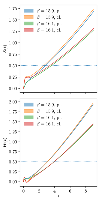
Figure 1: The quantities $\mathcal{E}(t)$ (top panel) and $\mathcal{W}(t)$ (bottom panel), defined in Eqs. (22) and (23), and in Eq. (25), respectively, in the $N_{c}=6$ ensembles with $\beta=15.9$ and $\beta=16.3$, as functions of the flow time $t$. Computations adopt the alternative choices of discretisation provided by the elementary plaquette (pl.) and the clover-leaf plaquette (cl.). The horizontal dashed line represents the choice ${\cal E}_{0}=0.5$, ${\cal W}_{0}=0.5$.

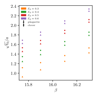
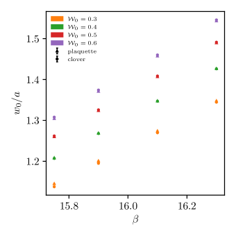
Figure 2: The gradient flow scales $\sqrt{t_{0}}/a$ (top panel) and $w_{0}/a$ (bottom) in $Sp(6)$, for different choices of $\mathcal{E}_{0}$ or ${\cal W}_{0}$, as a function of $\beta$, and comparing plaquette and clover discretisation. In the case of $w_{0}/a$, the difference between discretisations is barely discernible over the statistical uncertainty.

Each configuration in the ensembles in Table 1 sets the initial conditions for the numerical integration of the Wilson flow, which obeys Eq. (30). Following Ref. Luscher:2010iy , we use a third-order Runge-Kutta integrator (implemented by HiRep hirep-repo ) to evaluate $V_{\mu}(x,\,t)$ in the range $0<t<t_{\text{max}}$, with $t_{\text{max}}$ such that $\sqrt{8t_{\text{max}}}\lesssim L/2$, to avoid large finite size effects.

Table 2: The gradient flow scale $\sqrt{t_{0}}/a$ for different choices of $\beta$ and $\mathcal{E}_{0}$, for $N_{c}=6$. We report the results for both the plaquette and clover discretisations.

$\beta$	$\mathcal{E}_{0}$	$\sqrt{t_{0}}/a$ (pl.)	$\sqrt{t_{0}}/a$ (cl.)
$15.75$	$0.3$	$0.92442(25)$	$1.11491(20)$
$15.9$	$0.3$	$1.07199(36)$	$1.22045(33)$
$16.1$	$0.3$	$1.24921(48)$	$1.36866(47)$
$16.3$	$0.3$	$1.42716(42)$	$1.52798(41)$
$15.75$	$0.4$	$1.24407(31)$	$1.34614(29)$
$15.9$	$0.4$	$1.38876(49)$	$1.47758(49)$
$16.1$	$0.4$	$1.58507(71)$	$1.66099(69)$
$16.3$	$0.4$	$1.79128(63)$	$1.85737(60)$
$15.75$	$0.5$	$1.45355(39)$	$1.53196(37)$
$15.9$	$0.5$	$1.61449(63)$	$1.68380(63)$
$16.1$	$0.5$	$1.83487(92)$	$1.89487(89)$
$16.3$	$0.5$	$2.06770(82)$	$2.12034(78)$
$15.75$	$0.6$	$1.62169(46)$	$1.68890(44)$
$15.9$	$0.6$	$1.79810(76)$	$1.85783(76)$
$16.1$	$0.6$	$2.0401(11)$	$2.0920(11)$
$16.3$	$0.6$	$2.2960(10)$	$2.34178(95)$

Table 3: The gradient flow scale $w_{0}/a$ for different choices of $\beta$ and $\mathcal{W}_{0}$, for $N_{c}=6$. We report the results for both the plaquette and clover discretisations.

$\beta$	$\mathcal{W}_{0}$	$w_{0}/a$ (pl.)	$w_{0}/a$ (cl.)
$15.75$	$0.3$	$1.14525(18)$	$1.13768(17)$
$15.9$	$0.3$	$1.20091(29)$	$1.19500(29)$
$16.1$	$0.3$	$1.27407(40)$	$1.26968(38)$
$16.3$	$0.3$	$1.34793(34)$	$1.34454(32)$
$15.75$	$0.4$	$1.20835(21)$	$1.20698(20)$
$15.9$	$0.4$	$1.26876(33)$	$1.26784(33)$
$16.1$	$0.4$	$1.34754(46)$	$1.34701(44)$
$16.3$	$0.4$	$1.42652(39)$	$1.42624(37)$
$15.75$	$0.5$	$1.26030(23)$	$1.26195(22)$
$15.9$	$0.5$	$1.32419(37)$	$1.32572(37)$
$16.1$	$0.5$	$1.40712(51)$	$1.40852(48)$
$16.3$	$0.5$	$1.48995(43)$	$1.49123(41)$
$15.75$	$0.6$	$1.30458(25)$	$1.30797(24)$
$15.9$	$0.6$	$1.37126(40)$	$1.37421(40)$
$16.1$	$0.6$	$1.45758(55)$	$1.46009(53)$
$16.3$	$0.6$	$1.54353(47)$	$1.54572(45)$

The quantity ${\cal E}(t)$ is obtained from the definitions in Eqs. (22) and (23), by computing $G_{\mu\nu}$ from $B_{\mu}$. We use two alternative discretised expressions for ${\cal E}(t)$, provided by the plaquette (pl.), ${\cal P}_{\mu\nu}$, or the clover-leaf (cl.), ${\cal C}_{\mu\nu}$. We then compute ${\cal W}(t)$ according to Eq. (25). The resampled results for ${\cal E}(t)$ and ${\cal W}(t)$, as functions of $t$, are displayed in the two panels of Fig. 1, in the case $N_{c}=6$, with $\beta=15.9$ and $\beta=16.3$ and for the two different discretizations (pl. and cl.). For each value of $t$, the vertical thickness of the curves represents the error of ${\cal E}(t)$ and ${\cal W}(t)$, computed by bootstrapping. The picture is qualitatively the same for other values of the bare parameters and is similar to the $SU(N_{c})$ case.

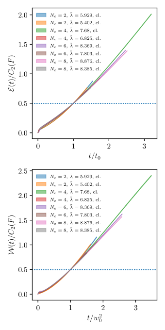
Figure 3: The quantities $\mathcal{E}(t)/C_{2}(F)$ (top panel) and $\mathcal{W}(t)/C_{2}(F)$ (bottom) computed with the clover-leaf plaquette discretisation of the flow equation on the available ensembles corresponding to the finest and coarsest available lattices, for each $N_{c}$, with $C_{2}(F)=(N_{c}+1)/4$, displayed as a function of the rescaled flow times $t/t_{0}$ and $t/w_{0}^{2}$. The figure adopts the choice $c_{e}=c_{w}=0.5$ (horizontal dashed line).

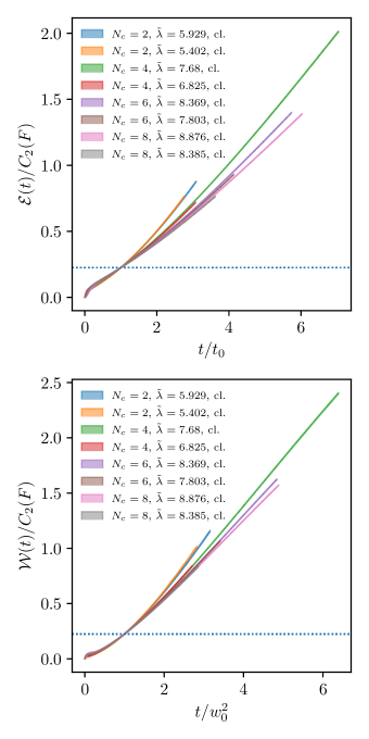
Figure 4: The quantities $\mathcal{E}(t)/C_{2}(F)$ (top panel) and $\mathcal{W}(t)/C_{2}(F)$ (bottom) computed with the clover-leaf plaquette discretisation of the flow equation on the available ensembles corresponding to the finest and coarsest lattices, for each $N_{c}$, with $C_{2}(F)=(N_{c}+1)/4$, displayed as a function of the rescaled flow times $t/t_{0}$ and $t/w_{0}^{2}$. The figure adopts the choice $c_{e}=c_{w}=0.225$ (horizontal dashed line).

From ${\cal E}(t)$ and ${\cal W}(t)$ we can extract the scales $t_{0}$ and $w_{0}$, according to the definitions in Eqs. (24) and (26), once we make a choice for the reference values ${\cal E}_{0}$ and ${\cal W}_{0}$. For illustrative purposes, the choices $\mathcal{E}_{0}=0.5$ and $\mathcal{W}_{0}=0.5$ are represented as horizontal dashed lines in the top and bottom panel of Fig. 1, though we do not use this choice in the analysis. The comparison between ${\cal E}(t)$ and ${\cal W}(t)$ provides a first assessment of the magnitude of discretisation effects in the calculation. For each ensemble, the difference between the curves corresponding to the plaquette and clover discretisations tends to a constant at large $t$. This difference is the smallest in the ensemble with the largest value of $\beta$—the closest to the continuum limit—and is smaller for ${\cal W}(t)$ than ${\cal E}(t)$, as anticipated in Section III.

A more refined assessment of discretisation effects can be obtained by studying the value of the scales $\sqrt{t_{0}}/a$ and $w_{0}/a$, obtained for a range of choices of ${\cal E}_{0}$ and ${\cal W}_{0}$, for each available ensemble, which we report in Tables 2 and 3, and display in Fig. 2 for $Sp(6)$. The difference between the plaquette and clover discretizsations becomes smaller as $\beta$ is increased. This difference has generally a smaller magnitude for the $w_{0}$ scale than for $\sqrt{t_{0}}$ scale. A similar picture emerges for $N_{c}=2$, $N_{c}=4$, and $N_{c}=8$. as reported in Appendix A. In view of these considerations, we adopt the clover discretisation in the following.

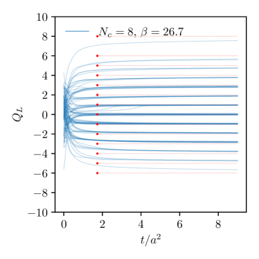
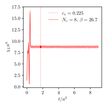
Figure 5: In the top panel, he topological charge $Q_{L}$ as a function of the flow time $t/a^{2}$, for the $100$ first configurations of the ensemble with $N_{c}=8$, $L/a=16$, and $\beta=26.7$. The values of $\tilde{Q}_{L}$ are also reported as red bullets at $t=t_{0}$, where $t_{0}$ is obtained from the choice $c_{e}=0.225$. In the bottom panel, the topological susceptibility $\chi_{L}(t)a^{4}$ as a function of the flow time $t$, with its $1$-$\sigma$ error band, for $N_{c}=8$, at $\beta=26.7$. The vertical dashed represents $t=t_{0}$, where $t_{0}$ is obtained from $c_{e}=c_{w}=0.225$. The value of $\chi_{L}(t=t_{0})a^{4}$ obtained at $t=t_{0}$ is depicted as a red bullet and reported in Table 4.

In Section III, we observed that the functions ${\cal E}(t)$ and ${\cal W}(t)$ obey perturbative relations that suggest the scaling bahaviour in Eq. (28). The numerical data we have collected allows to test the validity of these scaling relations outside of the domain of perturbation theory. We choose values of $\mathcal{E}_{0}$ and $\mathcal{W}_{0}$ for each value of $N_{c}$ according to Eq. (28), with fixed $c_{e}$ and $c_{w}$. The corresponding values of $t_{0}$ and $w_{0}$ are then used to scale also $t$.

The result of these operations, with the clover-leaf discretisation, and at each fixed value of $N_{c}$, for the ensembles with the smallest and the greatest values of $\beta$, are displayed in Fig. 3 for the choice $c_{e}=c_{w}=0.5$. The plots exhibit the same qualitative features for both ${\cal E}(t)/C_{2}(F)$ and ${\cal W}(t)/C_{2}(F)$ as functions of $t/t_{0}$ and $t/w_{0}^{2}$, respectively. We repeat the same process also for the choice $c_{e}=c_{w}=0.225$ (which would yield ${\cal E}_{0}=0.3$ for $SU(3)$), and display the results in Fig. 4. We labelled the curves by the conveniently defined discretised coupling

$$\tilde{\lambda} \equiv \frac{d_{G}}{\beta\left\langle\frac{\Re{\rm Tr\,}\mathcal{P}_{\mu\nu}}{2N}\right\rangle}\,,$$ (35)

where $d_{G}$ is the dimension of the group.

By construction, the rescaled flows corresponding to different values of $N_{c}$ coincide when $t/t_{0}=1$ (or $t/w_{0}^{2}=1$). What is interesting is that the curves agree (within uncertainties) over a sizeable range of $t$ around these points. This might indicate that the validity of the perturbative scaling in Eq. (28) holds also outside of the naive range of the perturbative regime. Small deviations from perfect scaling are nevertheless visible and might be ascribed to a combination of finite-$a$ and finite-$N_{c}$ effects.

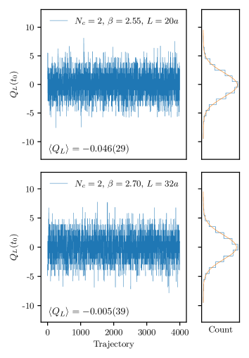
Figure 6: The topological charge $Q_{L}$ as a function of simulation time (trajectory) for the ensembles corresponding to the coarsest (top) and finest (bottom) lattice with $N_{c}=2$. The value of $Q_{L}$ is computed at $t=t_{0}$, where the value of $t_{0}$ is obtained from $c_{e}=0.225$. The average value of the topological charge along the trajectory is reported in the bottom left-hand side of plot. The side panel contains the cumulative histogram of the values of $Q_{L}(t_{0})$. The orange curve is a gaussian fit to the cumulative histogram.

IV.2 The topological charge

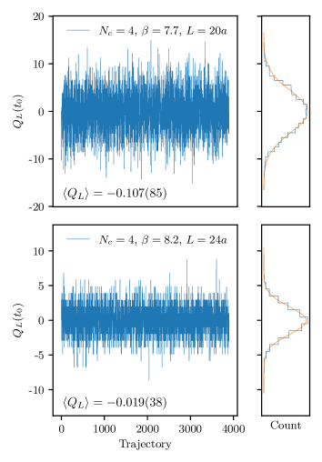
Figure 7: The topological charge $Q_{L}$ as a function of simulation time (trajectory) for the ensembles corresponding to the coarsest (top) and finest (bottom) lattice with $N_{c}=4$. The value of $Q_{L}$ is computed at $t=t_{0}$, where the value of $t_{0}$ is obtained from $c_{e}=0.225$. The average value of the topological charge along the trajectory is reported in the bottom left-hand side of plot. The side panel contains the cumulative histogram of the values of $Q_{L}(t_{0})$. The orange curve is a gaussian fit to the cumulative histogram.

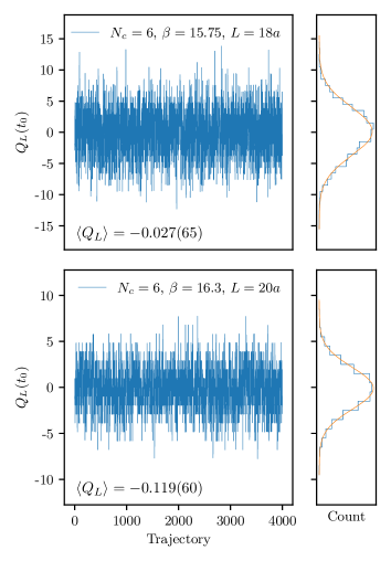
Figure 8: The topological charge $Q_{L}$ as a function of simulation time (trajectory) for the ensembles corresponding to the coarsest (top) and finest (bottom) lattice with $N_{c}=6$. The value of $Q_{L}$ is computed at $t=t_{0}$, where the value of $t_{0}$ is obtained from $c_{e}=0.225$. The average value of the topological charge along the trajectory is reported in the bottom left-hand side of plot. The side panel contains the cumulative histogram of the valuoThe orange curve is a gaussian fit to the cumulative histogram. es of $Q_{L}(t_{0})$.

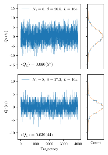
Figure 9: The topological charge $Q_{L}$ as a function of simulation time (trajectory) for the ensembles corresponding to the coarsest (top) and finest (bottom) lattice with $N_{c}=8$. The value of $Q_{L}$ is computed at $t=t_{0}$, where the value of $t_{0}$ is obtained from $c_{e}=0.225$. The average value of the topological charge along the trajectory is reported in the bottom left-hand side of plot. The side panel contains the cumulative histogram of the values of $Q_{L}(t_{0})$. The orange curve is a gaussian fit to the cumulative histogram.

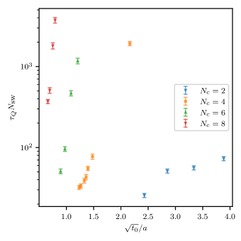
Figure 10: The integrated autocorrelation time $\tau_{Q}$ multiplied by the number of sweeps $N_{\rm sw}$, as a function of the scale $\sqrt{t_{0}}/a$, for $c_{e}=0.225$ for $N_{c}=2$, $4$, $6$, $8$.

The quantity $Q_{L}(t)$ is computed from Wilson-flowed configurations at flow time $t$, using Eq. (31), as implemented by HiRep hirep-repo . Fig. 5 is compiled with the first 100 configurations of the ensemble with $N_{c}=8$ and $\beta=26.7$. Integer values for $Q_{L}(t)$ are only obtained for $a\rightarrow 0$. At non-zero $a$, the quantity $Q_{L}(t)$ tends, at large $t$, towards quasi-integer values. The integer-valued topological charge $\tilde{Q}_{L}$ is instead obtained for a finite value of $t$, according to Eq. (32). The values of $\tilde{Q}_{L}$ are displayed in Fig. 5 as red bullets, and for the value of $t=t_{0}$ identified with the choice $c_{e}=0.225$. Effectively this definition of $\tilde{Q}_{L}$ optimises and expedites the convergence towards the physical, discrete values of the topological charge. Similar conclusions hold for other values of the bare parameters, though we do not report further details here. In the following, we will compute $\tilde{Q}_{L}$ for every configuration of every ensemble at both $c_{e}=0.225$ and $c_{e}=0.5$.

Simulation histories of $Q_{L}$ for the ensembles with the finest and coarsest lattice are displayed in Figs. 6, 7, 8, and 9, for $N_{c}=2,\,4,\,6,\,8,$ respectively. The frequency histogram for the values of $Q_{L}$ is also reported, in each case, and is consistent with a Gaussian, symmetric distribution around $Q_{L}=0$.

The magnitude of autocorrelations can be evaluated using the Madras-Sokal windowing algorithm Madras:1988ei on the simulation history of either $Q_{L}$ or $\tilde{Q}_{L}$. For our ensembles, we found no significant difference to arise between the two, and no visible dependence on the choice of $c_{e}$. We thus compute $\tau_{Q}$ at $t=t_{0}$, for $c_{e}=0.225$. The behaviour of the logarithm of $\tau_{Q}N_{sw}$ as a function of $\beta$ is displayed in Fig. 10 and reported in Table 1. On the basis of known results obtained for $SU(N_{c})$ gauge groups, $\ln\tau_{Q}N_{sw}$ is expected to be linearly diverging as $\beta\rightarrow\infty$ DelDebbio:2002xa , and indeed this is consistent with what we find.

Table 4: Topological susceptibilities $\chi_{L}t_{0}^{2}$ and $\chi_{L}w_{0}^{4}$, with $c_{e}=c_{w}=0.225$, and the string tensions $\sigma t_{0}$ and $\sigma w_{0}^{2}$, for all available ensembles. These results are displayed as a function of $a^{2}/{t_{0}}$ and $a^{2}/w_{0}^{2}$ in Figure 11.

$N_{c}$	$\beta$	$\sigma t_{0}$	$\chi_{L}t_{0}^{2}\cdot 10^{4}$	$\sigma w_{0}^{2}$	$\chi_{L}w_{0}^{4}\cdot 10^{4}$
$2$	$2.55$	$0.11440(93)$	$6.69(16)$	$0.11164(92)$	$6.40(15)$
$2$	$2.6$	$0.1120(11)$	$6.39(12)$	$0.1090(10)$	$6.07(14)$
$2$	$2.65$	$0.1120(20)$	$6.55(14)$	$0.1092(19)$	$6.21(14)$
$2$	$2.7$	$0.1097(18)$	$6.17(14)$	$0.1070(18)$	$5.87(17)$
$4$	$7.7$	$0.1029(24)$	$5.19(12)$	$0.1127(26)$	$6.47(15)$
$4$	$7.72$	$0.1035(28)$	$5.52(12)$	$0.1138(31)$	$6.80(16)$
$4$	$7.76$	$0.0987(29)$	$5.50(11)$	$0.1087(32)$	$6.71(16)$
$4$	$7.78$	$0.1028(29)$	$5.29(15)$	$0.1136(32)$	$6.44(15)$
$4$	$7.8$	$0.0988(23)$	$5.06(12)$	$0.1093(26)$	$6.16(15)$
$4$	$7.85$	$0.1013(14)$	$5.18(13)$	$0.1125(16)$	$6.40(16)$
$4$	$8.2$	$0.1036(16)$	$4.79(12)$	$0.1171(18)$	$6.11(15)$
$6$	$15.75$	$0.0972(12)$	$4.61(12)$	$0.1146(15)$	$6.36(15)$
$6$	$15.9$	$0.0988(13)$	$4.244(93)$	$0.1177(15)$	$5.98(13)$
$6$	$16.1$	$0.0947(16)$	$4.19(10)$	$0.1138(20)$	$6.06(15)$
$6$	$16.3$	$0.0955(33)$	$3.85(10)$	$0.1153(40)$	$5.61(15)$
$8$	$26.5$	$0.0953(13)$	$4.146(78)$	$0.1170(16)$	$6.27(11)$
$8$	$26.7$	$0.0954(26)$	$4.03(11)$	$0.1181(32)$	$6.16(17)$
$8$	$27.0$	$0.0942(14)$	$3.99(10)$	$0.1177(17)$	$6.23(18)$
$8$	$27.2$	$0.0905(13)$	$3.606(90)$	$0.1138(17)$	$5.72(18)$

Table 5: Topological susceptibilities $\chi_{L}t_{0}^{2}$ and $\chi_{L}w_{0}^{4}$, with $c_{e}=c_{w}=0.5$, and the string tensions $\sigma t_{0}$ and $\sigma w_{0}^{2}$, for all available ensembles. These results are displayed as a function of $a^{2}/{t_{0}}$ and $a^{2}/w_{0}^{2}$ in Figure 11.

$N_{c}$	$\beta$	$\sigma t_{0}$	$\chi_{L}t_{0}^{2}\cdot 10^{3}$	$\sigma w_{0}^{2}$	$\chi_{L}w_{0}^{4}\cdot 10^{3}$
$2$	$2.55$	$0.2289(19)$	$2.547(58)$	$0.1956(16)$	$1.881(47)$
$2$	$2.6$	$0.2235(21)$	$2.448(49)$	$0.1907(18)$	$1.789(35)$
$2$	$2.65$	$0.2233(39)$	$2.527(60)$	$0.1902(33)$	$1.840(40)$
$2$	$2.7$	$0.2186(37)$	$2.388(63)$	$0.1861(31)$	$1.736(45)$
$4$	$7.7$	$0.2265(52)$	$2.510(60)$	$0.2070(47)$	$2.100(51)$
$4$	$7.72$	$0.2281(62)$	$2.669(76)$	$0.2087(56)$	$2.246(56)$
$4$	$7.76$	$0.2178(63)$	$2.647(59)$	$0.1992(58)$	$2.225(46)$
$4$	$7.78$	$0.2271(64)$	$2.556(61)$	$0.2080(59)$	$2.137(57)$
$4$	$7.8$	$0.2186(51)$	$2.430(53)$	$0.2001(47)$	$2.040(48)$
$4$	$7.85$	$0.2246(31)$	$2.507(67)$	$0.2060(29)$	$2.113(53)$
$4$	$8.2$	$0.2323(36)$	$2.399(62)$	$0.2146(33)$	$2.055(47)$
$6$	$15.75$	$0.2261(29)$	$2.468(49)$	$0.2147(28)$	$2.221(50)$
$6$	$15.9$	$0.2313(30)$	$2.317(53)$	$0.2208(29)$	$2.103(47)$
$6$	$16.1$	$0.2230(38)$	$2.310(56)$	$0.2136(37)$	$2.126(53)$
$6$	$16.3$	$0.2254(78)$	$2.137(56)$	$0.2162(75)$	$1.975(60)$
$8$	$26.5$	$0.2285(31)$	$2.380(49)$	$0.2220(30)$	$2.248(45)$
$8$	$26.7$	$0.2301(63)$	$2.345(70)$	$0.2243(61)$	$2.230(65)$
$8$	$27.0$	$0.2285(33)$	$2.351(76)$	$0.2236(32)$	$2.244(66)$
$8$	$27.2$	$0.2204(32)$	$2.149(64)$	$0.2161(32)$	$2.057(51)$

The topological susceptibility in lattice units $\chi_{L}(t)a^{4}$ was computed for each ensemble separately, using Eq. (34). The effect of the rounding procedure, Eq. (32), on the topological susceptibility, is displayed in Figure 5, where $\chi_{L}(t)a^{4}$ is plotted as a function of the flow time $t/a^{2}$. For sufficiently large values of the flow time, $\chi_{L}(t)a^{4}$ is compatible with a constant within errors. The value of $\chi_{L}t_{0}^{2}$ computed at the scale $t_{0}$, obtained from $c_{e}=w_{e}=0.225$, is displayed as a red bullet. We report the results for the choices $c_{e}=c_{w}=0.225$ and $c_{e}=c_{w}=0.5$, in Tables 4 and 5, respectively. For convenience, we also report the values of $\sigma t_{0}$ and $\sigma w_{0}^{2}$, which are taken from Ref. Bennett:2020qtj , except for $\beta=2.55$, $2.65$ for $N_{c}=2$, and $\beta=7.72$, $7.76$, $7.78$ and $7.80$ for $N_{c}=4$, which we computed anew.

Table 6: Continuum limit extrapolations obtained from the best fit of Eq. (36) for the topological susceptibility in $Sp(N_{c})$ Yang-Mills theories with $N_{c}=2,\,4,\,6,\,8$. We present four alternative ways of setting the scale: we measure $\chi t_{0}^{2}(a=0)$ (top section of the table) and $\chi w_{0}^{4}(a=0)$ (bottom), and adopt as reference values either $c_{e}=0.225=c_{w}$ (left section of the table) or $c_{e}=0.5=c_{w}$ (right). The best-fit curves are displayed as dashed lines in Figure 11, for each value of $N_{c}$, along with the individual measurements.

$N_{c}$	$\chi_{L}t_{0}^{2}(a=0)$	$\tilde{\mathcal{X}}^{2}$	$\chi_{L}t_{0}^{2}(a=0)$	$\tilde{\mathcal{X}}^{2}$
	$c_{e}=0.225$		$c_{e}=0.5$
$2$	$0.000600(22)$	$1.47$	$0.002353(93)$	$1.29$
$4$	$0.000452(17)$	$2.18$	$0.002305(90)$	$1.89$
$6$	$0.000315(23)$	$1.08$	$0.00185(11)$	$1.02$
$8$	$0.000303(23)$	$2.32$	$0.00194(15)$	$1.39$
$N_{c}$	$\chi_{L}w_{0}^{4}(a=0)$	$\tilde{\mathcal{X}}^{2}$	$\chi_{L}w_{0}^{4}(a=0)$	$\tilde{\mathcal{X}}^{2}$
	$c_{w}=0.225$		$c_{w}=0.5$
$2$	$0.000572(24)$	$1.16$	$0.001698(69)$	$1.50$
$4$	$0.000584(22)$	$1.63$	$0.001991(69)$	$2.14$
$6$	$0.000503(32)$	$1.39$	$0.00180(12)$	$1.13$
$8$	$0.000535(39)$	$1.41$	$0.00189(13)$	$1.80$

Our final results are the extrapolations towards the continuum limit of $\chi_{L}t_{0}^{2}$ for each of the $Sp(N_{c})$ Yang-Mills theories. We obtain these by assuming the following functional dependence:

$$\chi_{L}(a)t_{0}^{2}=\chi_{L}(a=0)t_{0}^{2}+c_{1}\frac{a^{2}}{t_{0}}\,,$$ (36)

for each value of $N_{c}$, separately. The results of this extrapolation are reported in Table 6 (and displayed in Fig. 11) for $c_{e}=0.225$ and $c_{e}=0.5$, respectively. For completeness, we also report in the same Table 6 and Fig. 11 also the extrapolation of $\chi_{L}w_{0}^{2}$, obtained with a similar fitting function which includes one correction term ${\cal O}\left(\frac{a^{2}}{w_{0}^{2}}\right)$. The uncertainty on the extrapolated values are obtained from the maximum likelihood analysis by including statistical uncertainties only. Ref. Ce:2016awn , which reports $\chi t_{0}^{2}$ for $SU(N_{c})$ with $N_{c}=3,\,4,\,5,\,6$, present the results in units of $t_{0}$, and for the choice $c_{e}=0.225$. Unfortunately, a direct comparison is not possible, as the authors of Ref. Ce:2016awn did not report on the common $SU(2)\sim Sp(2)$ case. We will return to the comparison of the topological susceptibility in $Sp(N_{c})$ and $SU(N_{c})$ theories in a companion publication Bennett:2022gdz .

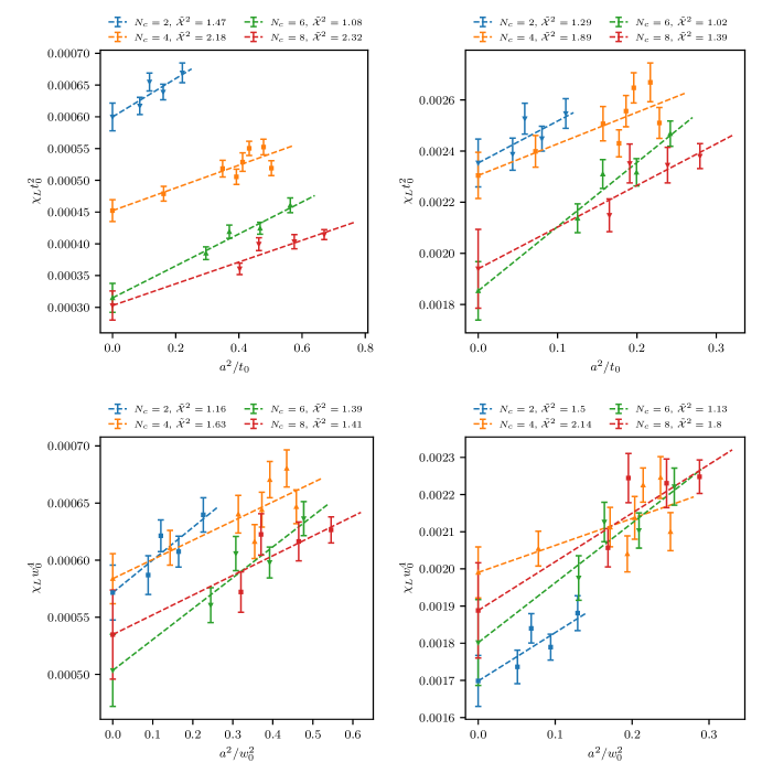
Figure 11: Topological susceptibility per unit volume $\chi_{L}t_{0}^{2}$ as a function of $a^{2}/t_{0}$ (top panels) and $\chi_{L}w_{0}^{4}$ as a function of $a^{2}/w_{0}^{2}$ (bottom), in $Sp(N_{c})$ Yang-Mills theories with $N_{c}=2,\,4,\,6,\,8$. We adopt reference values $c_{e}=c_{w}=0.225$ (left panels) and $c_{e}=c_{w}=0.5$ (right). Our continuum extrapolations are represented as dashed lines. The results are reported in Table 6.

V Summary and discussion

We studied the four-dimensional Yang-Mills theories with group $Sp(N_{c})$, for $N_{c}=2,\,4,\,6,\,8$, by means of lattice numerical techniques. We used the Wilson flow as a scale-setting procedure. We showed that lattice artefacts are reduced by adopting the clover-leaf plaquette discretisation. We also found that by simultaneously rescaling $\mathcal{E}(t)$ (or alternatively $\mathcal{W}(t)$), the reference value of $\mathcal{E}_{0}$ (or alternatively $\mathcal{W}_{0}$), and $t_{0}/a^{2}$ (or alternatively $w_{0}/a$), the Wilson flows for different gauge groups agree (within numerical errors) over a non-trivial range of $t$. The proposed rescaling is based upon the group-factor dependence of the leading-order perturbative evaluation of $\mathcal{E}(t)$, indicating that the suppression of sub-leading corrections that differentiate the groups holds also non-perturbatively, over a finite range of flow time $t$.

We then computed the topological susceptibility from our lattice ensembles, expressed it in units of the Wilson flow scale $t_{0}$ ($w_{0}$), and performed the continuum extrapolation for the four gauge groups. We summarise in Table 6 our results for the continuum extrapolation of $\chi t_{0}^{2}$ and $\chi w_{0}^{4}$ for two different choices of reference values for $\mathcal{E}_{0}$ and $\mathcal{W}_{0}$. In a companion paper Bennett:2022gdz , we present our extrapolation of the measurement of the topological susceptibility towards the large-$N_{c}$ limit (in units of the string tension), and discuss how to compare it with the analogous calculations performed for $SU(N_{c})$ Yang-Mills theories.

Appendix A Scale setting data for $N_{c}=2$, $4$, $8$

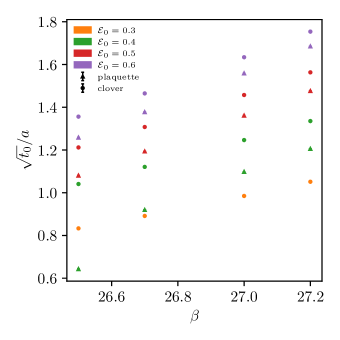
Figure 16: The gradient flow scale $\sqrt{t_{0}}/a$ in $Sp(8)$, for different choices of $\mathcal{E}_{0}$, as a function of $\beta$, and comparing plaquette and clover discretisation.

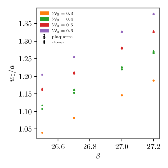
Figure 17: The gradient flow scale ${w_{0}}/a$ in $Sp(8)$, for different choices of $\mathcal{W}_{0}$, as a function of $\beta$, and comparing plaquette and clover discretisation.

In this Appendix, we report the intermediate results of the scale-setting procedure for the $Sp(2)$, $Sp(4)$, and $Sp(8)$ Yang-Mills theories. The presentation mirrors the one for the $Sp(6)$ theory, in the main body of the paper. Tables 7 and 8 present our results for $t_{0}/a^{2}$ and $w_{0}/a$, respectively, for various choices of reference values $\mathcal{E}_{0}$ and $\mathcal{W}_{0}$, for $N_{c}=2$. We tabulate the results for both the plaquette and clover discretisations. Tables 9 and 10 list the same information, but for $Sp(4)$, while Tables 11 and 12 refer to $Sp(8)$. Cases in which Eqs. (24) or (26) do not admit a solution, because of extreme choices of ${\cal E}_{0}$ or ${\cal W}_{0}$, are left blank. The information in Tables 7-12 is also graphically displayed in Figs. 12–17, and available in machine-readable form in Ref. datapackage .

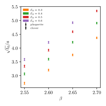
Figure 12: The gradient flow scale $\sqrt{t_{0}}/a$ in $Sp(2)$, for different choices of $\mathcal{E}_{0}$, as a function of $\beta$, and comparing plaquette and clover discretisation.

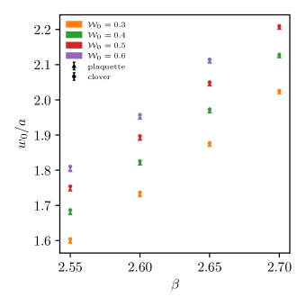
Figure 13: The gradient flow scale ${w_{0}}/a$ in $Sp(2)$, for different choices of $\mathcal{W}_{0}$, as a function of $\beta$, and comparing plaquette and clover discretisation.

Table 7: The gradient flow scale $\sqrt{t_{0}}/a$ for different choices of $\mathcal{E}_{0}$ and $\beta$, for $N_{c}=2$. We report the results for both the plaquette and clover discretisations.

$\beta$	$\mathcal{E}_{0}$	$\sqrt{t_{0}}/a$ (pl.)	$\sqrt{t_{0}}/a$ (cl.)
$2.55$	$0.3$	$2.6989(30)$	$2.7489(29)$
$2.60$	$0.3$	$3.1810(33)$	$3.2244(32)$
$2.65$	$0.3$	$3.7340(29)$	$3.7714(30)$
$2.70$	$0.3$	$4.3570(48)$	$4.3900(46)$
$2.55$	$0.4$	$3.0384(36)$	$3.0883(34)$
$2.60$	$0.4$	$3.5774(40)$	$3.6209(38)$
$2.65$	$0.4$	$4.1958(36)$	$4.2335(36)$
$2.70$	$0.4$	$4.8929(57)$	$4.9263(55)$
$2.55$	$0.5$	$3.3189(41)$	$3.3694(40)$
$2.60$	$0.5$	$3.9040(46)$	$3.9484(43)$
$2.65$	$0.5$	$4.5761(41)$	$4.6146(41)$
$2.70$	$0.5$	$5.3333(66)$	$5.3680(64)$
$2.55$	$0.6$	$3.5614(47)$	$3.6131(45)$
$2.60$	$0.6$	$4.1864(51)$	$4.2320(48)$
$2.65$	$0.6$	$4.9040(46)$	$4.9438(46)$
$2.70$	$0.6$	$-$	$-$

Table 8: The gradient flow scale $w_{0}/a$ for different choices of $\mathcal{W}_{0}$ as a function of $\beta$, for $N_{c}=2$. We report the results for both the plaquette and clover discretisations.

$\beta$	$\mathcal{W}_{0}$	$w_{0}/a$ (pl.)	$w_{0}/a$ (cl.)
$2.55$	$0.3$	$1.5961(11)$	$1.6046(10)$
$2.60$	$0.3$	$1.7292(11)$	$1.7366(10)$
$2.65$	$0.3$	$1.87188(92)$	$1.87785(90)$
$2.70$	$0.3$	$2.0210(14)$	$2.0260(13)$
$2.55$	$0.4$	$1.6776(12)$	$1.6868(11)$
$2.60$	$0.4$	$1.8185(13)$	$1.8260(12)$
$2.65$	$0.4$	$1.9669(10)$	$1.9732(10)$
$2.70$	$0.4$	$2.1235(16)$	$2.1287(15)$
$2.55$	$0.5$	$1.7448(13)$	$1.7541(13)$
$2.60$	$0.5$	$1.8889(14)$	$1.8973(13)$
$2.65$	$0.5$	$2.0435(11)$	$2.0502(11)$
$2.70$	$0.5$	$2.2045(18)$	$2.2102(16)$
$2.55$	$0.6$	$1.8002(15)$	$1.8104(14)$
$2.60$	$0.6$	$1.9487(14)$	$1.9576(14)$
$2.65$	$0.6$	$2.1082(13)$	$2.1151(12)$
$2.70$	$0.6$	$-$	$-$

Table 9: The gradient flow scale $\sqrt{t_{0}}/a$ for different choices of $\mathcal{E}_{0}$ and $\beta$, for $N_{c}=4$. We report the results for both the plaquette and clover discretisations.

$\beta$	$\mathcal{E}_{0}$	$\sqrt{t_{0}}/a$ (pl.)	$\sqrt{t_{0}}/a$ (cl.)
$7.7$	$0.3$	$1.37620(40)$	$1.46197(40)$
$7.72$	$0.3$	$1.41690(43)$	$1.49953(42)$
$7.76$	$0.3$	$1.49948(50)$	$1.57652(50)$
$7.78$	$0.3$	$1.54145(54)$	$1.61595(53)$
$7.80$	$0.3$	$1.58361(60)$	$1.65573(57)$
$7.85$	$0.3$	$1.68978(70)$	$1.75659(67)$
$7.7$	$0.4$	$1.62985(53)$	$1.69845(52)$
$7.72$	$0.4$	$1.67629(55)$	$1.74253(55)$
$7.76$	$0.4$	$1.77067(65)$	$1.83274(65)$
$7.78$	$0.4$	$1.81913(70)$	$1.87920(70)$
$7.80$	$0.4$	$1.86744(78)$	$1.92574(75)$
$7.85$	$0.4$	$1.99001(92)$	$2.04422(88)$
$7.7$	$0.5$	$1.82938(63)$	$1.89073(62)$
$7.72$	$0.5$	$1.88069(66)$	$1.94002(66)$
$7.76$	$0.5$	$1.98496(78)$	$2.04067(77)$
$7.78$	$0.5$	$2.03884(84)$	$2.09278(84)$
$7.80$	$0.5$	$2.09229(94)$	$2.14469(91)$
$7.85$	$0.5$	$2.2286(11)$	$2.2774(11)$
$7.7$	$0.6$	$1.99738(73)$	$2.05499(71)$
$7.72$	$0.6$	$2.05290(76)$	$2.10871(76)$
$7.76$	$0.6$	$2.16562(90)$	$2.21813(89)$
$7.78$	$0.6$	$2.22422(97)$	$2.27504(97)$
$7.80$	$0.6$	$2.2821(11)$	$2.3315(10)$
$7.85$	$0.6$	$2.4302(13)$	$2.4762(12)$

Table 10: The gradient flow scale $w_{0}/a$ for different choices of $\mathcal{W}_{0}$ as a function of $\beta$, for $N_{c}=4$. We report the results for both the plaquette and clover discretisations.

$\beta$	$\mathcal{W}_{0}$	$w_{0}/a$ (pl.)	$w_{0}/a$ (cl.)
$7.7$	$0.3$	$1.22784(24)$	$1.23049(24)$
$7.72$	$0.3$	$1.24453(25)$	$1.24707(25)$
$7.76$	$0.3$	$1.27680(29)$	$1.27933(28)$
$7.78$	$0.3$	$1.29372(31)$	$1.29613(30)$
$7.80$	$0.3$	$1.30975(34)$	$1.31216(32)$
$7.85$	$0.3$	$1.35073(39)$	$1.35299(37)$
$7.7$	$0.4$	$1.29494(27)$	$1.30037(27)$
$7.72$	$0.4$	$1.31252(28)$	$1.31777(28)$
$7.76$	$0.4$	$1.34674(33)$	$1.35169(32)$
$7.78$	$0.4$	$1.36470(35)$	$1.36940(34)$
$7.80$	$0.4$	$1.38167(38)$	$1.38628(37)$
$7.85$	$0.4$	$1.42523(44)$	$1.42944(42)$
$7.7$	$0.5$	$1.34954(30)$	$1.35640(29)$
$7.72$	$0.5$	$1.36784(31)$	$1.37449(30)$
$7.76$	$0.5$	$1.40345(36)$	$1.40970(35)$
$7.78$	$0.5$	$1.42221(38)$	$1.42816(38)$
$7.80$	$0.5$	$1.43994(41)$	$1.44572(40)$
$7.85$	$0.5$	$1.48552(49)$	$1.49076(47)$
$7.7$	$0.6$	$1.39593(33)$	$1.40365(32)$
$7.72$	$0.6$	$1.41485(33)$	$1.42232(33)$
$7.76$	$0.6$	$1.45159(39)$	$1.45864(38)$
$7.78$	$0.6$	$1.47110(42)$	$1.47776(41)$
$7.80$	$0.6$	$1.48942(44)$	$1.49585(44)$
$7.85$	$0.6$	$1.53659(53)$	$1.54244(51)$

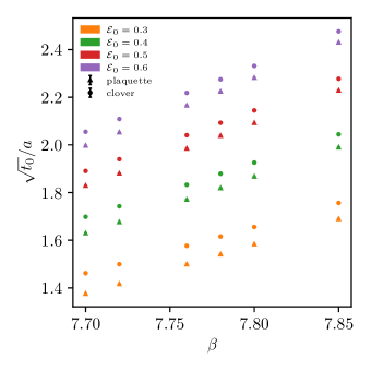
Figure 14: The gradient flow scale $\sqrt{t_{0}}/a$ in $Sp(4)$, for different choices of $\mathcal{E}_{0}$, as a function of $\beta$, and comparing plaquette and clover discretisation.

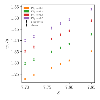
Figure 15: The gradient flow scale ${w_{0}}/a$ in $Sp(4)$, for different choices of $\mathcal{W}_{0}$, as a function of $\beta$, and comparing plaquette and clover discretisation.

Table 11: The gradient flow scale $\sqrt{t_{0}}/a$ for different choices of $\mathcal{E}_{0}$ and $\beta$, for $N_{c}=8$. We report the results for both the plaquette and clover discretisations.

$\beta$	$\mathcal{E}_{0}$	$\sqrt{t_{0}}/a$ (pl.)	$\sqrt{t_{0}}/a$ (cl.)
$26.5$	$0.3$	$-$	$-$
$26.7$	$0.3$	$-$	$-$
$27.0$	$0.3$	$-$	$-$
$27.2$	$0.3$	$-$	$-$
$26.5$	$0.4$	$0.6428(11)$	$1.04083(17)$
$26.7$	$0.4$	$0.91955(26)$	$1.12079(20)$
$27.0$	$0.4$	$1.09768(30)$	$1.24650(27)$
$27.2$	$0.4$	$1.20530(34)$	$1.33540(35)$
$26.5$	$0.5$	$1.08015(25)$	$1.21190(23)$
$26.7$	$0.5$	$1.19344(27)$	$1.30764(27)$
$27.0$	$0.5$	$1.36119(40)$	$1.45737(38)$
$27.2$	$0.5$	$1.47602(46)$	$1.56329(49)$
$26.5$	$0.6$	$1.25801(30)$	$1.35615(28)$
$26.7$	$0.6$	$1.37719(33)$	$1.46475(34)$
$27.0$	$0.6$	$1.55864(49)$	$1.63417(47)$
$27.2$	$0.6$	$1.68496(57)$	$1.75412(61)$

Table 12: The gradient flow scale $w_{0}/a$ for different choices of $\mathcal{W}_{0}$ as a function of $\beta$, for $N_{c}=8$. We report the results for both the plaquette and clover discretisations.

$\beta$	$\mathcal{W}_{0}$	$w_{0}/a$ (pl.)	$w_{0}/a$ (cl.)
$26.5$	$0.3$	$-$	$-$
$26.7$	$0.3$	$-$	$-$
$27.0$	$0.3$	$-$	$-$
$27.2$	$0.3$	$-$	$-$
$26.5$	$0.4$	$1.11790(16)$	$1.10726(15)$
$26.7$	$0.4$	$1.16124(17)$	$1.15275(18)$
$27.0$	$0.4$	$1.22617(25)$	$1.21983(24)$
$27.2$	$0.4$	$1.27059(28)$	$1.26524(30)$
$26.5$	$0.5$	$1.16496(18)$	$1.16048(17)$
$26.7$	$0.5$	$1.21151(19)$	$1.20807(20)$
$27.0$	$0.5$	$1.28068(28)$	$1.27826(27)$
$27.2$	$0.5$	$1.32779(31)$	$1.32582(34)$
$26.5$	$0.6$	$1.20570(19)$	$1.20466(18)$
$26.7$	$0.6$	$1.25467(21)$	$1.25407(22)$
$27.0$	$0.6$	$1.32710(31)$	$1.32690(29)$
$27.2$	$0.6$	$1.37632(34)$	$1.37627(37)$

References

- (1) A. Hietanen, R. Lewis, C. Pica and F. Sannino, “Fundamental Composite Higgs Dynamics on the Lattice: SU(2) with Two Flavors,” JHEP 1407, 116 (2014) doi:10.1007/JHEP07(2014)116 [arXiv:1404.2794 [hep-lat]].
- (2) W. Detmold, M. McCullough and A. Pochinsky, “Dark nuclei. II. Nuclear spectroscopy in two-color QCD,” Phys. Rev. D 90, no. 11, 114506 (2014) doi:10.1103/PhysRevD.90.114506 [arXiv:1406.4116 [hep-lat]].
- (3) R. Arthur, V. Drach, M. Hansen, A. Hietanen, C. Pica and F. Sannino, “SU(2) gauge theory with two fundamental flavors: A minimal template for model building,” Phys. Rev. D 94, no. 9, 094507 (2016) doi:10.1103/PhysRevD.94.094507 [arXiv:1602.06559 [hep-lat]].
- (4) R. Arthur, V. Drach, A. Hietanen, C. Pica and F. Sannino, “ Gauge Theory with Two Fundamental Flavours: Scalar and Pseudoscalar Spectrum,” arXiv:1607.06654 [hep-lat].
- (5) C. Pica, V. Drach, M. Hansen and F. Sannino, “Composite Higgs Dynamics on the Lattice,” EPJ Web Conf. 137, 10005 (2017) doi:10.1051/epjconf/201713710005 [arXiv:1612.09336 [hep-lat]].
- (6) J. W. Lee, B. Lucini and M. Piai, “Symmetry restoration at high-temperature in two-color and two-flavor lattice gauge theories,” JHEP 1704, 036 (2017) doi:10.1007/JHEP04(2017)036 [arXiv:1701.03228 [hep-lat]].
- (7) V. Drach, T. Janowski and C. Pica, “Update on SU(2) gauge theory with NF = 2 fundamental flavours,” EPJ Web Conf. 175, 08020 (2018) doi:10.1051/epjconf/201817508020 [arXiv:1710.07218 [hep-lat]].
- (8) V. Drach, T. Janowski, C. Pica and S. Prelovsek, “Scattering of Goldstone Bosons and resonance production in a Composite Higgs model on the lattice,” JHEP 04, 117 (2021) doi:10.1007/JHEP04(2021)117 [arXiv:2012.09761 [hep-lat]].
- (9) V. Drach, P. Fritzsch, A. Rago and F. Romero-López, “Singlet channel scattering in a Composite Higgs model on the lattice,” [arXiv:2107.09974 [hep-lat]].
- (10) E. Bennett, D. K. Hong, J. W. Lee, C.-J. D. Lin, B. Lucini, M. Piai and D. Vadacchino, “Sp(4) gauge theory on the lattice: towards SU(4)/Sp(4) composite Higgs (and beyond),” JHEP 1803, 185 (2018) doi:10.1007/JHEP03(2018)185 [arXiv:1712.04220 [hep-lat]].
- (11) J. W. Lee, E. Bennett, D. K. Hong, C. J. D. Lin, B. Lucini, M. Piai and D. Vadacchino, “Progress in the lattice simulations of Sp(2) gauge theories,” PoS LATTICE 2018, 192 (2018) doi:10.22323/1.334.0192 [arXiv:1811.00276 [hep-lat]].
- (12) E. Bennett, D. K. Hong, J. W. Lee, C. J. D. Lin, B. Lucini, M. Piai and D. Vadacchino, “Sp(4) gauge theories on the lattice: dynamical fundamental fermions,” JHEP 12 (2019), 053 doi:10.1007/JHEP12(2019)053 [arXiv:1909.12662 [hep-lat]].
- (13) E. Bennett, D. K. Hong, J. W. Lee, C. J. D. Lin, B. Lucini, M. Mesiti, M. Piai, J. Rantaharju and D. Vadacchino, “ gauge theories on the lattice: quenched fundamental and antisymmetric fermions,” Phys. Rev. D 101 (2020) no.7, 074516 doi:10.1103/PhysRevD.101.074516 [arXiv:1912.06505 [hep-lat]].
- (14) E. Bennett, J. Holligan, D. K. Hong, J. W. Lee, C. J. D. Lin, B. Lucini, M. Piai and D. Vadacchino, “Color dependence of tensor and scalar glueball masses in Yang-Mills theories,” Phys. Rev. D 102, no.1, 011501 (2020) doi:10.1103/PhysRevD.102.011501 [arXiv:2004.11063 [hep-lat]].
- (15) E. Bennett, J. Holligan, D. K. Hong, J. W. Lee, C. J. D. Lin, B. Lucini, M. Piai and D. Vadacchino, “Glueballs and strings in Yang-Mills theories,” Phys. Rev. D 103 (2021) no.5, 054509 doi:10.1103/PhysRevD.103.054509 [arXiv:2010.15781 [hep-lat]].
- (16) E. Bennett, D. K. Hong, H. Hsiao, J. W. Lee, C. J. D. Lin, B. Lucini, M. Mesiti, M. Piai and D. Vadacchino, “Lattice studies of the gauge theory with two fundamental and three antisymmetric Dirac fermions,” [arXiv:2202.05516 [hep-lat]].
- (17) E. Bennett, D. K. Hong, H. Hsiao, J. W. Lee, C. J. D. Lin, B. Lucini, M. Piai, and D. Vadacchino, “Sp(4) theories on the lattice: dynamical antisymmetric fermions,” in preparation.
- (18) J. Barnard, T. Gherghetta and T. S. Ray, “UV descriptions of composite Higgs models without elementary scalars,” JHEP 1402, 002 (2014) doi:10.1007/JHEP02(2014)002 [arXiv:1311.6562 [hep-ph]].
- (19) D. B. Kaplan and H. Georgi, “SU(2) x U(1) Breaking by Vacuum Misalignment,” Phys. Lett. B 136, 183-186 (1984) doi:10.1016/0370-2693(84)91177-8
- (20) H. Georgi and D. B. Kaplan, “Composite Higgs and Custodial SU(2),” Phys. Lett. 145B, 216 (1984). doi:10.1016/0370-2693(84)90341-1
- (21) M. J. Dugan, H. Georgi and D. B. Kaplan, “Anatomy of a Composite Higgs Model,” Nucl. Phys. B 254, 299 (1985). doi:10.1016/0550-3213(85)90221-4
- (22) D. B. Kaplan, “Flavor at SSC energies: A New mechanism for dynamically generated fermion masses,” Nucl. Phys. B 365 (1991), 259-278 doi:10.1016/S0550-3213(05)80021-5
- (23) G. Panico and A. Wulzer, “The Composite Nambu-Goldstone Higgs,” Lect. Notes Phys. 913, pp.1 (2016) doi:10.1007/978-3-319-22617-0 [arXiv:1506.01961 [hep-ph]].
- (24) O. Witzel, “Review on Composite Higgs Models,” PoS LATTICE 2018, 006 (2019) doi:10.22323/1.334.0006 [arXiv:1901.08216 [hep-lat]].
- (25) G. Cacciapaglia, C. Pica and F. Sannino, “Fundamental Composite Dynamics: A Review,” Phys. Rept. 877, 1-70 (2020) doi:10.1016/j.physrep.2020.07.002 [arXiv:2002.04914 [hep-ph]].
- (26) G. Ferretti and D. Karateev, “Fermionic UV completions of Composite Higgs models,” JHEP 03, 077 (2014) doi:10.1007/JHEP03(2014)077 [arXiv:1312.5330 [hep-ph]].
- (27) G. Ferretti, “Gauge theories of Partial Compositeness: Scenarios for Run-II of the LHC,” JHEP 06, 107 (2016) doi:10.1007/JHEP06(2016)107 [arXiv:1604.06467 [hep-ph]].
- (28) G. Cacciapaglia, G. Ferretti, T. Flacke and H. Serôdio, “Light scalars in composite Higgs models,” Front. Phys. 7, 22 (2019) doi:10.3389/fphy.2019.00022 [arXiv:1902.06890 [hep-ph]].
- (29) Y. Hochberg, E. Kuflik, T. Volansky and J. G. Wacker, “Mechanism for Thermal Relic Dark Matter of Strongly Interacting Massive Particles,” Phys. Rev. Lett. 113, 171301 (2014) doi:10.1103/PhysRevLett.113.171301 [arXiv:1402.5143 [hep-ph]].
- (30) Y. Hochberg, E. Kuflik, H. Murayama, T. Volansky and J. G. Wacker, “Model for Thermal Relic Dark Matter of Strongly Interacting Massive Particles,” Phys. Rev. Lett. 115, no.2, 021301 (2015) doi:10.1103/PhysRevLett.115.021301 [arXiv:1411.3727 [hep-ph]].
- (31) Y. Hochberg, E. Kuflik and H. Murayama, “SIMP Spectroscopy,” JHEP 05, 090 (2016) doi:10.1007/JHEP05(2016)090 [arXiv:1512.07917 [hep-ph]].
- (32) D. Kondo, R. McGehee, T. Melia and H. Murayama, [arXiv:2205.08088 [hep-ph]].
- (33) N. Bernal, X. Chu and J. Pradler, “Simply split strongly interacting massive particles,” Phys. Rev. D 95, no.11, 115023 (2017) doi:10.1103/PhysRevD.95.115023 [arXiv:1702.04906 [hep-ph]].
- (34) A. Berlin, N. Blinov, S. Gori, P. Schuster and N. Toro, “Cosmology and Accelerator Tests of Strongly Interacting Dark Matter,” Phys. Rev. D 97, no.5, 055033 (2018) doi:10.1103/PhysRevD.97.055033 [arXiv:1801.05805 [hep-ph]].
- (35) N. Bernal, X. Chu, S. Kulkarni and J. Pradler, “Self-interacting dark matter without prejudice,” Phys. Rev. D 101, no.5, 055044 (2020) doi:10.1103/PhysRevD.101.055044 [arXiv:1912.06681 [hep-ph]].
- (36) H. Cai and G. Cacciapaglia, “Singlet dark matter in the SU(6)/SO(6) composite Higgs model,” Phys. Rev. D 103, no.5, 055002 (2021) doi:10.1103/PhysRevD.103.055002 [arXiv:2007.04338 [hep-ph]].
- (37) Y. D. Tsai, R. McGehee and H. Murayama, “Resonant Self-Interacting Dark Matter from Dark QCD,” [arXiv:2008.08608 [hep-ph]].
- (38) A. Maas and F. Zierler, “Strong isospin breaking in Sp(4) gauge theory,” [arXiv:2109.14377 [hep-lat]].
- (39) F. Zierler and A. Maas, “ SIMP Dark Matter on the Lattice,” PoS LHCP2021, 162 (2021) doi:10.22323/1.397.0162
- (40) S. Kulkarni, A. Maas, S. Mee, M. Nikolic, J. Pradler and F. Zierler, “Low-energy effective description of dark theories,” [arXiv:2202.05191 [hep-ph]].
- (41) K. Holland, M. Pepe and U. J. Wiese, “The Deconfinement phase transition of Sp(2) and Sp(3) Yang-Mills theories in (2+1)-dimensions and (3+1)-dimensions,” Nucl. Phys. B 694, 35-58 (2004) doi:10.1016/j.nuclphysb.2004.06.026 [arXiv:hep-lat/0312022 [hep-lat]].
- (42) J. M. Maldacena, “The Large N limit of superconformal field theories and supergravity,” Int. J. Theor. Phys. 38, 1113 (1999) [Adv. Theor. Math. Phys. 2, 231 (1998)] doi:10.1023/A:1026654312961, 10.4310/ATMP.1998.v2.n2.a1 [hep-th/9711200].
- (43) S. S. Gubser, I. R. Klebanov and A. M. Polyakov, “Gauge theory correlators from noncritical string theory,” Phys. Lett. B 428, 105 (1998) doi:10.1016/S0370-2693(98)00377-3 [hep-th/9802109].
- (44) E. Witten, “Anti-de Sitter space and holography,” Adv. Theor. Math. Phys. 2, 253 (1998) doi:10.4310/ATMP.1998.v2.n2.a2 [hep-th/9802150].
- (45) O. Aharony, S. S. Gubser, J. M. Maldacena, H. Ooguri and Y. Oz, “Large N field theories, string theory and gravity,” Phys. Rept. 323, 183 (2000) doi:10.1016/S0370-1573(99)00083-6 [hep-th/9905111].
- (46) B. Lucini and M. Teper, “SU(N) gauge theories in four-dimensions: Exploring the approach to N = infinity,” JHEP 06 (2001), 050 doi:10.1088/1126-6708/2001/06/050 [arXiv:hep-lat/0103027 [hep-lat]].
- (47) B. Lucini, M. Teper and U. Wenger, “Glueballs and k-strings in SU(N) gauge theories: Calculations with improved operators,” JHEP 06, 012 (2004) doi:10.1088/1126-6708/2004/06/012 [arXiv:hep-lat/0404008 [hep-lat]].
- (48) B. Lucini, A. Rago and E. Rinaldi, “Glueball masses in the large N limit,” JHEP 08 (2010), 119 doi:10.1007/JHEP08(2010)119 [arXiv:1007.3879 [hep-lat]].
- (49) B. Lucini and M. Panero, “SU(N) gauge theories at large N,” Phys. Rept. 526, 93-163 (2013) doi:10.1016/j.physrep.2013.01.001 [arXiv:1210.4997 [hep-th]].
- (50) A. Athenodorou, R. Lau and M. Teper, “On the weak N -dependence of SO(N) and SU(N) gauge theories in 2+1 dimensions,” Phys. Lett. B 749, 448-453 (2015) doi:10.1016/j.physletb.2015.08.023 [arXiv:1504.08126 [hep-lat]].
- (51) R. Lau and M. Teper, “SO(N) gauge theories in 2 + 1 dimensions: glueball spectra and confinement,” JHEP 10, 022 (2017) doi:10.1007/JHEP10(2017)022 [arXiv:1701.06941 [hep-lat]].
- (52) D. K. Hong, J. W. Lee, B. Lucini, M. Piai and D. Vadacchino, “Casimir scaling and Yang–Mills glueballs,” Phys. Lett. B 775, 89-93 (2017) doi:10.1016/j.physletb.2017.10.050 [arXiv:1705.00286 [hep-th]].
- (53) N. Yamanaka, A. Nakamura and M. Wakayama, “Interglueball potential in lattice SU(N) gauge theories,” [arXiv:2110.04521 [hep-lat]].
- (54) P. Hernández and F. Romero-López, “The large limit of QCD on the lattice,” Eur. Phys. J. A 57, no.2, 52 (2021) doi:10.1140/epja/s10050-021-00374-2 [arXiv:2012.03331 [hep-lat]].
- (55) A. Athenodorou and M. Teper, “SU(N) gauge theories in 3+1 dimensions: glueball spectrum, string tensions and topology,” [arXiv:2106.00364 [hep-lat]].
- (56) C. Bonanno, M. D’Elia, B. Lucini and D. Vadacchino, “Towards glueball masses of large- pure-gauge theories without topological freezing,” [arXiv:2205.06190 [hep-lat]].
- (57) E. Witten, “Current Algebra Theorems for the U(1) Goldstone Boson,” Nucl. Phys. B 156, 269-283 (1979) doi:10.1016/0550-3213(79)90031-2
- (58) G. Veneziano, “U(1) Without Instantons,” Nucl. Phys. B 159, 213-224 (1979) doi:10.1016/0550-3213(79)90332-8
- (59) L. Del Debbio, H. Panagopoulos and E. Vicari, “theta dependence of SU(N) gauge theories,” JHEP 08, 044 (2002) doi:10.1088/1126-6708/2002/08/044 [arXiv:hep-th/0204125 [hep-th]].
- (60) B. Lucini, M. Teper and U. Wenger, “Topology of SU(N) gauge theories at T =~ 0 and T =~ T(c),” Nucl. Phys. B 715 (2005), 461-482 doi:10.1016/j.nuclphysb.2005.02.037 [arXiv:hep-lat/0401028 [hep-lat]].
- (61) L. Del Debbio, L. Giusti and C. Pica, “Topological susceptibility in the SU(3) gauge theory,” Phys. Rev. Lett. 94, 032003 (2005) doi:10.1103/PhysRevLett.94.032003 [arXiv:hep-th/0407052 [hep-th]].
- (62) M. Luscher and F. Palombi, “Universality of the topological susceptibility in the SU(3) gauge theory,” JHEP 09, 110 (2010) doi:10.1007/JHEP09(2010)110 [arXiv:1008.0732 [hep-lat]].
- (63) H. Panagopoulos and E. Vicari, “The 4D SU(3) gauge theory with an imaginary term,” JHEP 11, 119 (2011) doi:10.1007/JHEP11(2011)119 [arXiv:1109.6815 [hep-lat]].
- (64) C. Bonati, M. D’Elia and A. Scapellato, “ dependence in Yang-Mills theory from analytic continuation,” Phys. Rev. D 93, no.2, 025028 (2016) doi:10.1103/PhysRevD.93.025028 [arXiv:1512.01544 [hep-lat]].
- (65) M. Cè, M. Garcίa Vera, L. Giusti and S. Schaefer, “The topological susceptibility in the large- limit of SU() Yang–Mills theory,” Phys. Lett. B 762, 232-236 (2016) doi:10.1016/j.physletb.2016.09.029 [arXiv:1607.05939 [hep-lat]].
- (66) C. Bonati, M. D’Elia, P. Rossi and E. Vicari, “ dependence of 4D gauge theories in the large- limit,” Phys. Rev. D 94, no.8, 085017 (2016) doi:10.1103/PhysRevD.94.085017 [arXiv:1607.06360 [hep-lat]].
- (67) C. Alexandrou, A. Athenodorou, K. Cichy, A. Dromard, E. Garcia-Ramos, K. Jansen, U. Wenger and F. Zimmermann, “Comparison of topological charge definitions in Lattice QCD,” Eur. Phys. J. C 80 (2020) no.5, 424 doi:10.1140/epjc/s10052-020-7984-9 [arXiv:1708.00696 [hep-lat]].
- (68) C. Bonanno, C. Bonati and M. D’Elia, “Large- Yang-Mills theories with milder topological freezing,” JHEP 03, 111 (2021) doi:10.1007/JHEP03(2021)111 [arXiv:2012.14000 [hep-lat]].
- (69) S. Borsanyi and D. Sexty, “Topological susceptibility of pure gauge theory using Density of States,” Phys. Lett. B 815, 136148 (2021) doi:10.1016/j.physletb.2021.136148 [arXiv:2101.03383 [hep-lat]].
- (70) G. Cossu, D. Lancastera, B. Lucini, R. Pellegrini and A. Rago, “Ergodic sampling of the topological charge using the density of states,” Eur. Phys. J. C 81, no.4, 375 (2021) doi:10.1140/epjc/s10052-021-09161-1 [arXiv:2102.03630 [hep-lat]].
- (71) M. Teper, “More methods for calculating the topological charge (density) of SU(N) lattice gauge fields in 3+1 dimensions,” [arXiv:2202.02528 [hep-lat]].
- (72) E. Vicari and H. Panagopoulos, “Theta dependence of SU(N) gauge theories in the presence of a topological term,” Phys. Rept. 470 (2009), 93-150 doi:10.1016/j.physrep.2008.10.001 [arXiv:0803.1593 [hep-th]].
- (73) B. Lucini, E. Bennett, J. Holligan, D. K. Hong, H. Hsiao, J. W. Lee, C. J. D. Lin, M. Mesiti, M. Piai and D. Vadacchino, “Sp(4) gauge theories and beyond the standard model physics,” [arXiv:2111.12125 [hep-lat]].
- (74) E. Bennett, J. Holligan, D. K. Hong, H. Hsiao, J. W. Lee, C. J. D. Lin, B. Lucini, M. Mesiti, M. Piai and D. Vadacchino, “Progress in lattice gauge theories,” [arXiv:2111.14544 [hep-lat]].
- (75) Bennett, D. K. Hong, J. W. Lee, C. J. D. Lin, B. Lucini, M. Piai and D. Vadacchino, “Color dependence of the topological susceptibility in Yang-Mills theories,” [arXiv:2205.09254 [hep-lat]].
- (76) M. Lüscher, “Properties and uses of the Wilson flow in lattice QCD,” JHEP 08, 071 (2010) [erratum: JHEP 03, 092 (2014)] doi:10.1007/JHEP08(2010)071 [arXiv:1006.4518 [hep-lat]].
- (77) M. Lüscher, “Future applications of the Yang-Mills gradient flow in lattice QCD,” PoS LATTICE2013, 016 (2014) doi:10.22323/1.187.0016 [arXiv:1308.5598 [hep-lat]].
- (78) B. Sheikholeslami and R. Wohlert, “Improved Continuum Limit Lattice Action for QCD with Wilson Fermions,” Nucl. Phys. B 259, 572 (1985) doi:10.1016/0550-3213(85)90002-1
- (79) M. Hasenbusch and K. Jansen, “Speeding up lattice QCD simulations with clover improved Wilson fermions,” Nucl. Phys. B 659, 299-320 (2003) doi:10.1016/S0550-3213(03)00227-X [arXiv:hep-lat/0211042 [hep-lat]].
- (80) https://github.com/sa2c/HiRep.
- (81) L. Del Debbio, A. Patella and C. Pica, “Higher representations on the lattice: Numerical simulations. SU(2) with adjoint fermions,” Phys. Rev. D 81 (2010), 094503 doi:10.1103/PhysRevD.81.094503 [arXiv:0805.2058 [hep-lat]].
- (82) M. Campostrini, A. Di Giacomo, H. Panagopoulos and E. Vicari, “Topological Charge, Renormalization and Cooling on the Lattice,” Nucl. Phys. B 329, 683-697 (1990) doi:10.1016/0550-3213(90)90077-Q
- (83) M. Luscher, “Topology of Lattice Gauge Fields,” Commun. Math. Phys. 85, 39 (1982) doi:10.1007/BF02029132
- (84) M. Luscher and S. Schaefer, “Lattice QCD without topology barriers,” JHEP 07, 036 (2011) doi:10.1007/JHEP07(2011)036 [arXiv:1105.4749 [hep-lat]].
- (85) M. G. Endres, R. C. Brower, W. Detmold, K. Orginos and A. V. Pochinsky, “Multiscale Monte Carlo equilibration: Pure Yang-Mills theory,” Phys. Rev. D 92, no.11, 114516 (2015) doi:10.1103/PhysRevD.92.114516 [arXiv:1510.04675 [hep-lat]].
- (86) M. Lüscher, “Stochastic locality and master-field simulations of very large lattices,” EPJ Web Conf. 175, 01002 (2018) doi:10.1051/epjconf/201817501002 [arXiv:1707.09758 [hep-lat]].
- (87) S. Borsanyi, S. Durr, Z. Fodor, C. Hoelbling, S. D. Katz, S. Krieg, T. Kurth, L. Lellouch, T. Lippert and C. McNeile, et al. “High-precision scale setting in lattice QCD,” JHEP 09 (2012), 010 doi:10.1007/JHEP09(2012)010 [arXiv:1203.4469 [hep-lat]].
- (88) E. Bennett, D. K. Hong, J. W. Lee, C. J. D. Lin, B. Lucini, M. Piai, and D. Vadacchino, “ Yang-Mills theories on the lattice: scale setting and topology—data release”, doi: https://doi.org/10.5281/zenodo.6678411
- (89) E. Bennett, D. K. Hong, J. W. Lee, C. J. D. Lin, B. Lucini, M. Piai, and D. Vadacchino, “ Yang-Mills theories on the lattice: scale setting and topology—analysis workflow”, doi: https://doi.org/10.5281/zenodo.6685967
- (90) N. Madras and A. D. Sokal, “The Pivot algorithm: a highly efficient Monte Carlo method for selfavoiding walk,” J. Statist. Phys. 50, 109-186 (1988) doi:10.1007/BF01022990