Self radiation force on a moving monopolar source

Abstract

The radiation force exerted on an object by an acoustic wave is a widely studied phenomenon since the early work of Rayleigh, Langevin and Brillouin and has led in the last decade to tremendous developments for acoustic micromanipulation. Despite extensive work on this phenomenon, the expressions of the acoustic radiation force applied on a particle have so far been derived only for a steady particle, hence neglecting the effect of its displacement on the radiated wave. In this work we study the acoustic radiation force exerted on a monopolar source translating at a constant velocity small compared to the sound speed. We demonstrate that the asymmetry of the emitted field resulting from Doppler effect induces a radiation force on the source opposite to its motion.

1 Introduction

Since the seminal work by Rayleigh (1902, 1905) and Langevin (work reported later by Biquard (1932a, b)), much effort has been devoted to the derivation of theoretical expressions of the acoustic radiation force exerted by an acoustic wave on a particle. Brillouin (1925b, a) was the first to recognize the tensorial nature of the acoustic radiation force, which is not necessarily orthogonal to the insonified interface. Later on, King (1934) derived an expression of the axial acoustic radiation force exerted on a rigid spherical particle by a plane wave. This expression was extended to the case of a compressible fluid sphere and of an elastic particle by Yosika & Kawasima (1955) and Hasegawa & Yosika (1969) respectively. The case of an incident focused wave was treated by Embleton (1954) for a rigid particle and Chen & Apfel (1996) for an elastic particle. Later on, the more general case of the axial force exerted by a Bessel beam was addressed by Marston (2006, 2009).

In parallel, a general expression of the acoustic radiation force exerted by an arbitrary wavefield on a spherical particle in the Long Wavelength Regime (LWR i.e. when $ka\ll 1$ with $k$ the wavenumber and $a$ the particle radius) was obtained by Gork’ov (1962). It was shown up to 3rd order (in $ka$) that the radiation force is proportional to the gradient of an acoustic potential, which is proportional to the difference between the time-averaged potential and kinetic acoustic energy weighed respectively by the monopole and dipole scattering coefficients. This expression was extended to the 6th order by Sapozhnikov & Bailey (2013), which is necessary when the average potential and kinetic energy are uniform in space (e.g. for plane propagating waves). This expression was also extended by Doinikov (1997a, b, c) to consider the effect of the viscous and thermal boundary layers in some asymptotic limits (of the boundary layer size compared to the particle size) and in the general case by Settnes & Bruus (2012) and Karlsen & Bruus (2015). The case of nonspherical particles such as disks and spheroids was treated by Keller (1957) and Silva & Drinkwater (2018) respectively, while the case of transient acoustic fields was recently addressed by Wang et al. (2021). We can also note that some expression for the secondary radiation force (inter-particle force) have been derived by Silva & Bruus (2011). The specific case of the radiation force exerted on a vibrating bubble known as the primary Bjerkness force was treated separately by Bjerknes (1906), Blake (1949), Eller (1968) and Crum (1975). Indeed, bubbles have some specificity: owing to their strong compressibility compared to the surrounding liquid, their monopolar resonance appears in the LWR. Hence bubbles can be attracted to the nodes or anti-nodes of a standing wave depending whether they are forced below or above their monopolar resonance frequency (see Eller (1968)).

Recently, there have been some renewed interest in the calculation of the acoustic radiation force with the development of selective acoustical tweezers (see Baudoin & Thomas (2020) for a review of the subject). Acoustical tweezers rely on the acoustic radiation force to move objects. To reach selectivity, i.e. the ability to manipulate a single object independently of other neighboring objects, it is necessary to localize the acoustic energy close to the target particle to only affect it (see e.g. Baresch et al. (2016), Baudoin et al. (2019),Baudoin et al. (2020)). Hence, such selectivity cannot be reached in the LWR. In addition, to calculate the restoring force (i.e. the force which brings back the particle toward the trap center), it is necessary to compute the radiation force when the particle is out-centered from the trap position. Yet, all the aforementioned expressions were either limited to the calculation of the radiation force for an axisymmetric configuration or to the LWR. To cope with this issue, general expressions of the radiation force exerted by an arbitrary incident field on a spherical particle, without restriction on the particle size compared to the wavelength, were obtained by Sapozhnikov & Bailey (2013) with an angular spectrum based method and by Silva (2011), and Baresch et al. (2013) with a multipole expansion method. The equivalence between the formula obtained with the different approaches was demonstrated by Gong & Baudoin (2021). Note also that some general expressions have been proposed to compute the acoustic radiation torque exerted by an arbitrary acoustic field on a particle of arbitrary size by Silva et al. (2012) and Gong & Baudoin (2020).

Yet, in all the theoretical developments mentioned so far, the calculation of the radiation force is made for a steady particle, hence neglecting the effect of its motion. Some account of the interaction between the oscillatory and translational motion of bubbles can be found in the literature. Following Saffman (1967), Benjamin & Ellis (1990) showed that even in an inviscid fluid, self-propulsion of a bubble can be achieved by nonlinear interactions between adjacent surface deformation modes. In their work however, the surface modes deformation are supposed to be known a priori. This work was extended later on by Mei & Zhou (1991) to account for the parametric excitation of surface modes by the isotropic volume mode and Feng & Leal (1995) who considered the direct coupling between translational motion, volume and shape modes. Finally, Doinikov (2004) obtained an expression of this coupling whatever the shape modes, their natural frequency, and the type of excitation (parametric forcing by the volume mode or direct excitation through externally induced pressure gradients at the surface of the bubble). In parallel it was also shown by Watanabe & Kukita (1993) and Doinikov (2002) that even if the bubble oscillations remain spherical, some complex coupling between volumetric oscillations and translational motion leading to erratic motion of the bubble can still occur when the bubble is excited by acoustic standing waves of high intensity. Finally, we can mention the work of Magnaudet & Legendre (1998) who computed how the viscous drag applied on a translating bubble is modified by its oscillation.

But none of these works considered the effect of the asymmetry of the acoustic wave radiated by a translating source on the acoustic radiation force. In this paper, we consider a monopolar source translating in a quiescent inviscid fluid at a constant velocity $U$ along a fixed axis and demonstrate that the asymmetry of the acoustic field due to Doppler effect (Figure 1) induces a self-induced radiation force on the source resisting its motion. This result is obtained by inserting the well known solution of the wavefield radiated by a moving monopolar source into a far-field integral expression of the radiation force exerted on a moving source, and finally computing this integral within the approximation of slow translating speed compared to the sound speed.

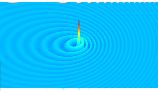
Figure 1: Sketch illustrating the asymmetry of the acoustic field synthesized by a translating monopolar source. The normalized field is calculated with eq. (21) and for the sake of illustration, the asymmetry is magnified by choosing a Mach number M = 0.5.

2 Wavefield radiated by a translating monopolar source

The first step to compute the self-induced radiation force exerted on a moving monopolar source is to compute the wavefield radiated by this source in a fixed reference frame. This classic calculation can be found in the acoustics textbook of Morse & Ingard (1968). In this first section, we recall the main steps of the derivation. Here we suppose the fluid to be inviscid.

2.1 Wave equation for a translating monopolar source

In acoustics, a monopolar source can be seen as a source of mass, whose strength is specified by the instantaneous mass flow rate $q(t)$ created by this source. In the following, the source is supposed to be periodic of period T. For a punctual source translating at a velocity $\mathbf{U}=U\mathbf{x}=Mc_{o}\,\mathbf{x}$ along a fixed axis $\mathbf{x}$, the mass and momentum conservation equations become:

$$\frac{\partial\rho}{\partial t}+\mathbf{\nabla}\cdot\left(\rho\mathbf{v}\right)=q(t)\delta(x-Mc_{0}t)\delta(y)\delta(z),$$ (1)

$$\frac{\partial\rho\mathbf{v}}{\partial t}+\mathbf{\nabla}\left(\rho\mathbf{v}\otimes\mathbf{v}\right)=\mathbf{\nabla}\bar{\bar{\sigma}},$$ (2)

with $\mathcal{R}=(O,(x,y,z),t)$ a Galilean reference frame, $M$ the mach number, $c_{o}$ the sound speed, $\rho$ the density, $\mathbf{v}$ the fluid velocity, $\bar{\bar{\sigma}}$ the stress tensor equal to $-p\bar{\bar{I}}$ for an inviscid fluid, $\bar{\bar{I}}$ the identity tensor and $p$ the pressure. If we (i) make the classic asymptotic development of equations (1) and (2) up to first order:

$$\rho=\rho_{0}+\epsilon\,\rho_{1}$$ (3a)

$$p=p_{0}+\epsilon\,p_{1}$$ (3b)

$$\mathbf{v}=\mathbf{v}_{o}+\epsilon\,\mathbf{v}_{1}$$ (3c)

with $\epsilon\ll 1$, and obtain the linearized mass and momentum balance:

$$\frac{\partial\rho_{1}}{\partial t}+\rho_{0}\mathbf{\nabla}\cdot\mathbf{v_{1}}=q(t)\delta(x-Mc_{0}t)\delta(y)\delta(z),$$ (4)

$$\rho_{0}\frac{\partial\mathbf{v_{1}}}{\partial t}=-\mathbf{\nabla}p_{1},$$ (5)

(ii) introduce the sound speed:

$$c_{0}^{2}=\left(\frac{\partial p}{\partial\rho}\right)_{s}=\frac{p_{1}}{\rho_{1}},$$ (6)

where $s$ is the entropy and (iii) combine the time derivative of equation (4) with the divergence of equation (5), we obtain the wave equation:

$$\Delta p_{1}-\frac{1}{c_{0}^{2}}\frac{\partial^{2}p_{1}}{\partial t^{2}}=-\frac{\partial}{\partial t}\left[q(t)\delta(x-Mc_{0}t)\delta(y)\delta(z)\right].$$ (7)

Note that to ease the resolution of this problem, it is convenient to introduce the velocity potential $\psi_{1}$ defined by $\mathbf{v_{1}}=-\frac{1}{\rho_{0}}\mathbf{\nabla}\psi_{1}$ such that $p_{1}=\frac{\partial\psi_{1}}{\partial t}$, which enables to suppress the time derivative in the rhs of equation (7):

$$\Delta\psi_{1}-\frac{1}{c_{0}^{2}}\frac{\partial^{2}\psi_{1}}{\partial t^{2}}=-q(t)\delta(x-Mc_{0}t)\delta(y)\delta(z),$$ (8)

and will make the future change of variables easier.

2.2 Resolution of the wave equation and Lorentz transformation

The solution of the wave equation (8) is well-known for a fixed monopolar source ($M=0$):

$$\psi_{1}(r,t)=\frac{q(t\pm r/c_{0})}{4\pi r},$$ (9)

with $r=\sqrt{x^{2}+y^{2}+z^{2}}$ the radial distance. To solve the problem for the moving source, the idea is to rewrite equation (8) in a reference frame wherein the source is fixed and the wave equation remains unchanged. This can be achieved by using the invariance of the wave equation by the Lorentz transformation, which is at the core of special relativity:

$$x^{\prime}=\gamma\left(x-Mc_{0}t\right)$$ (10a)

$$y^{\prime}=y$$ (10b)

$$z^{\prime}=z$$ (10c)

$$c_{0}t^{\prime}=\gamma\left(c_{0}t-Mx\right),$$ (10d)

where $\gamma$ defined by $\gamma^{-1}=\sqrt{1-M^{2}}$ is the ”Lorentz acoustic boost”. With this transformation, the wave equation (8) becomes:

$$\Delta^{\prime}\psi_{1}-\frac{1}{c_{0}^{2}}\frac{\partial^{2}\psi_{1}}{\partial t^{\prime 2}}=-q\left(\gamma(t^{\prime}+Mx^{\prime}/c)\right)\delta(x^{\prime}/\gamma)\delta(y^{\prime})\delta(z^{\prime}).$$ (11)

Since the rhs of equation (11) is null when $x^{\prime}\neq 0$ for all $t^{\prime}$ and using $\delta(x^{\prime}/\gamma)=\gamma\delta(x^{\prime})$, it comes:

$$\Delta^{\prime}\psi_{1}-\frac{1}{c_{0}^{2}}\frac{\partial^{2}\psi_{1}}{\partial t^{\prime 2}}=-\gamma q(\gamma t^{\prime})\delta(x^{\prime})\delta(y^{\prime})\delta(z^{\prime}).$$ (12)

If we now introduce a second set of variables:

$$x^{\prime\prime}=\gamma x^{\prime}$$ (13a)

$$y^{\prime\prime}=\gamma y^{\prime}$$ (13b)

$$z^{\prime\prime}=\gamma z^{\prime}$$ (13c)

$$c_{0}t^{\prime\prime}=\gamma c_{0}t^{\prime},$$ (13d)

the wave equation becomes:

$$\Delta^{\prime\prime}\psi_{1}-\frac{1}{c_{0}^{2}}\frac{\partial^{2}\psi_{1}}{\partial t^{\prime\prime 2}}=-\gamma^{2}q(t^{\prime\prime})\delta(x^{\prime\prime})\delta(y^{\prime\prime})\delta(z^{\prime\prime}),$$ (14)

which now resembles the static monopolar source problem and whose solution is:

$$\psi_{1}(r^{\prime\prime},t^{\prime\prime})=\gamma^{2}\frac{q(t^{\prime\prime}\pm r^{\prime\prime}/c_{0})}{4\pi r^{\prime\prime}}.$$ (15)

If we now perform the inverse transformations to obtain the potential as a function of $(x,y,z,t)$, we obtain:

$$\psi_{1}(r^{\prime},t^{\prime})=\gamma^{2}\frac{q(\gamma(t^{\prime}\pm r^{\prime}/c_{0}))}{4\pi\gamma r^{\prime}},$$ (16)

with:

$$\gamma(t^{\prime}\pm\frac{r^{\prime}}{c_{0}}) = \frac{\gamma}{c_{0}}\left[\gamma(c_{0}t-Mx)\pm\sqrt{[\gamma(x-Mc_{0}t)]^{2}+y^{2}+z^{2}}\right]$$ (17)

$$= t-\frac{M(x-Mc_{0}t)\pm\sqrt{(x-Mc_{0}t)^{2}+(y^{2}+z^{2})(1-M^{2})}}{c_{0}(1-M^{2})},$$ (18)

If we introduce the distance $R_{\pm}$ between the emission and the observation points:

$$R_{\pm}=\frac{M(x-Mc_{0}t)\pm R_{1}}{1-M^{2}},$$ (19)

with

$$R_{1}=\sqrt{(x-Mc_{0}t)^{2}+(y^{2}+z^{2})(1-M^{2})},$$ (20)

then the solution becomes:

$$\boxed{\psi_{1}(r,t)=\frac{q(t-R/c_{0})}{4\pi R_{1}},}$$ (21)

with $R=R_{+}$ in the subsonic case ($M<1$).

3 Integral expression of the radiation stress in the far field

The next step is to derive a far-field integral expression of the radiation stress exerted on a moving source. Indeed in acoustics, a monopolar point source constitutes a far-field approximation of a real source of finite extent and hence the above expressions are only valid in the far field.

Figure 2: $\mathcal{S}$ represents the source surface, varying over time. The surface $\mathcal{S_{\infty}}$ is centered on the source and moves with it at the velocity $\mathbf{U}$ in $\mathcal{R}$. $\mathcal{R}^{*}$ is the frame of the source.

3.1 Far field expression of the radiation force for a moving source

The acoustic radiation stress exerted on an object of surface $\mathcal{S}(t)$ is by definition the time average of the surface integral of the stress exerted by the acoustic wave on its surface:

$$\left<\mathbf{F}_{\text{rad}}\right>=\left<\iint_{\mathcal{S}(t)}\bar{\bar{\sigma}}\mathbf{n}dS\right>,$$ (22)

where $\left<f\right>=\frac{1}{T}\int_{t}^{t+T}f(t)dt$ is the time average of the function $f$ and T the period of the function $f(t)$. In general, there are two difficulties when computing this integral: (i) the surface of the object is vibrating and hence depends on time ($\mathcal{S}=\mathcal{S}(t)$) and (ii) an expression of the wave scattered by the object in the near field must be known. Hence generally this integral is converted into an integral over a closed surface at rest surrounding the object in the far field by using the divergence theorem and Reynolds transport theorem (see e.g. the review by Baudoin & Thomas (2020) for details of this process). Here an additional difficulty comes from the fact that the particle, in addition to its vibration, is translating at a constant velocity $U$. To solve this issue, we will transpose our integral of the stress on the surface of the object into an integral over a spherical surface $\mathcal{S_{\infty}}$ of radius $r_{\infty}\gg\lambda$, centered on the source, and hence translating at the velocity $\mathbf{U}$ in $\mathcal{R}$ (see Figure 2), with $\lambda=c_{0}/f$ the wavelength and $f$ the frequency. The volume between $\mathcal{S}$ and $\mathcal{S_{\infty}}$ is named $\mathcal{V}$. The integral of equation (2) over $\mathcal{V}$ gives:

$$\iiint_{\mathcal{V}}{\left[\frac{\partial\rho\mathbf{v}}{\partial t}+\mathbf{\nabla}\left(\rho\mathbf{v}\otimes\mathbf{v}-\bar{\bar{\sigma}}\right)\right]dV}=\mathbf{0}.$$ (23)

Using the divergence theorem, this volume integral turns into:

$$\iiint_{\mathcal{V}}{\frac{\partial\rho\mathbf{v}}{\partial t}dV}-\iint_{\mathcal{S}}\left(\rho\mathbf{v}\otimes\mathbf{v}-\bar{\bar{\sigma}}\right)\mathbf{n}dS+\iint_{\mathcal{S_{\infty}}}\left(\rho\mathbf{v}\otimes\mathbf{v}-\bar{\bar{\sigma}}\right)\mathbf{n_{\infty}}dS=\mathbf{0},$$ (24)

with $\mathbf{n}$ and $\mathbf{n_{\infty}}$ the outgoing normal vectors to the surface $\mathcal{S}$ and $\mathcal{S_{\infty}}$ respectively (see Figure 2). Another equation can be obtained by applying the Reynolds transport theorem to the momentum density $\rho\mathbf{v}$:

$$\frac{d}{dt}\iiint_{\mathcal{V}}{\rho\mathbf{v}dV}=\iiint_{\mathcal{V}}{\frac{\partial\rho\mathbf{v}}{\partial t}dV}-\iint_{\mathcal{S}}(\mathbf{v}\cdot\mathbf{n})\rho\mathbf{v}dS+\iint_{\mathcal{S_{\infty}}}(\mathbf{U}\cdot\mathbf{n_{\infty}})\rho\mathbf{v}dS,$$ (25)

since the surface $\mathcal{S}$ follows the object surface displacement (equal to the fluid displacement at the interface due to the continuity condition) and the surface $\mathcal{S_{\infty}}$ is translating at a constant velocity $\mathbf{v}$. If we study the steady regime, then:

$$\left<\frac{d}{dt}\iiint_{\mathcal{V}}{\rho\mathbf{v}dV}\right>=\mathbf{0}.$$ (26)

Finally, if we substract the time average of equation (25) to the time average of equation (24) and take into account (26), we obtain:

$$\left<\mathbf{F}_{\text{rad}}\right>=\left<\iint_{\mathcal{S_{\infty}}}\left(\bar{\bar{\sigma}}-\rho\mathbf{v}\otimes\mathbf{v}\right)\mathbf{n_{\infty}}dS\right>+\left<\iint_{\mathcal{S_{\infty}}}(\mathbf{U}\cdot\mathbf{n_{\infty}})\rho\mathbf{v}dS\right>.$$ (27)

3.2 Expression as a function of the first order acoustic field

In order to compute the previous integrals and since the time average of first order terms are equal to $\mathbf{0}$ for a periodic signal, we need to express the terms appearing in equation (27) up to second order. Here we suppose again that the fluid is inviscid and hence $\bar{\bar{\sigma}}=-p\bar{\bar{I}}$. If we push the asymptotic development up to second order:

$$\rho=\rho_{0}+\epsilon\rho_{1}+\epsilon^{2}\rho_{2}$$ (28a)

$$p=p_{0}+\epsilon p_{1}+\epsilon^{2}p_{2}$$ (28b)

$$\mathbf{v}=\epsilon\mathbf{v_{1}}+\epsilon^{2}\mathbf{v_{2}},$$ (28c)

the momentum balance (2) at second order in the volume $\mathcal{V}$ becomes:

$$\rho_{0}\frac{\partial\mathbf{v_{2}}}{\partial t}+\rho_{1}\frac{\partial\mathbf{v_{1}}}{\partial t}+\rho_{0}\left(\mathbf{v_{1}}\mathbf{\nabla}\mathbf{v_{1}}\right)=-\mathbf{\nabla}p_{2}.$$ (29)

If we take the time-average of this equation, we obtain:

$$\left<-\mathbf{\nabla}p_{2}\right>=\left<\rho_{1}\frac{\partial\mathbf{v_{1}}}{\partial t}+\rho_{0}\left(\mathbf{v_{1}}\mathbf{\nabla}\mathbf{v_{1}}\right)\right>,$$ (30)

since $\left<\frac{\partial\mathbf{v_{2}}}{\partial t}\right>=\mathbf{0}$ in the steady regime. From the first order momentum conservation (5), we have $\frac{\partial\mathbf{v_{1}}}{\partial t}=-\frac{1}{\rho_{0}}\nabla p_{1}$ and from the state equation (6) we have $\rho_{1}=p_{1}/c_{0}^{2}$ leading to:

$$\rho_{1}\frac{\partial\mathbf{v_{1}}}{\partial t}=-\frac{1}{2\rho_{0}c_{0}^{2}}\mathbf{\nabla}p_{1}^{2}.$$ (31)

And since the acoustic field is by definition irrotationnal:

$$\rho_{0}\left(\mathbf{v_{1}}\mathbf{\nabla}\mathbf{v_{1}}\right)=\frac{\rho_{0}}{2}\mathbf{\nabla}\mathbf{v_{1}}^{2}.$$ (32)

Finally, by replacing (31) and (32) in (30), we obtain:

$$\left<-\mathbf{\nabla}p_{2}\right>=\left<-\frac{1}{2\rho_{0}c_{0}^{2}}\mathbf{\nabla}p_{1}^{2}+\frac{\rho_{0}}{2}\mathbf{\nabla}\mathbf{v_{1}}^{2}\right>.$$ (33)

From this equation, we obtain the second order averaged stress tensor:

$$\left<\bar{\bar{\sigma}}_{2}\right>=-\left<p_{2}\bar{\bar{I}}\right>=\left<\left(\rho_{0}\frac{v_{1}^{2}}{2}-\frac{1}{\rho_{0}c_{0}^{2}}\frac{p_{1}^{2}}{2}\right)\bar{\bar{I}}\right>.$$ (34)

Then at second order, we have:

$$\left<\rho\mathbf{v}\otimes\mathbf{v}\right>=\left<\rho_{0}\mathbf{v_{1}}\otimes\mathbf{v_{1}}\right>$$ (35)

$$\left<\rho\mathbf{v}\right>=\left<\rho_{1}\mathbf{v_{1}}\right>,$$ (36)

so that if we replace equations (34), (35) and (36) in (27), we obtain the final expression of the radiation force as a function of the first order acoustic fields:

$$\boxed{\left<\mathbf{F}_{\text{rad}}\right>=\left<\iint_{\mathcal{S_{\infty}}}{\left[\left(\rho_{0}\frac{v_{1}^{2}}{2}-\frac{1}{\rho_{0}c_{0}^{2}}\frac{p_{1}^{2}}{2}\right)\bar{\bar{I}}-\rho_{0}\mathbf{v_{1}}\otimes\mathbf{v_{1}}\right]}\mathbf{n}dS\right>+\left<\iint_{\mathcal{S_{\infty}}}(\mathbf{U}\cdot\mathbf{n_{\infty}})\rho_{1}\mathbf{v_{1}}dS\right>.}$$ (37)

4 Expression of the radiation force for a slowly translating source

The final step is to compute this integral from the first order acoustic field.

4.1 Pressure, density and velocity fields at first order

The first step to compute equation (37) is to determine the pressure, density and velocity fields at first order from the expression of the velocity potential determined previously (equation (21)). First,

$$p_{1}=\frac{\partial\psi_{1}}{\partial t}=\frac{(1-\frac{1}{c_{0}}\frac{\partial R}{\partial t})q^{\prime}(t-R/c_{0})}{4\pi R_{1}}-\frac{q(t-R/c_{0})\frac{\partial R_{1}}{\partial t}}{4\pi R_{1}^{2}}.$$ (38)

Moreover, the coordinate of the velocity $v_{1i}$ along the direction $x_{i}=(x,y,z)$ is:

$$v_{1x_{i}}=-\frac{1}{\rho_{0}}\frac{\partial\psi_{1}}{\partial x_{i}}=-\frac{1}{\rho_{0}}\left(\frac{-\frac{1}{c_{0}}\frac{\partial R}{\partial x_{i}}q^{\prime}(t-R/c_{0})}{4\pi R_{1}}-\frac{q(t-R/c_{0})\frac{\partial R_{1}}{\partial x_{i}}}{4\pi R_{1}^{2}}\right).$$ (39)

Of course, we have: $\rho_{1}=p_{1}/c_{0}^{2}$. Here $R$ and $R_{1}$ are time and space dependent functions. To simplify the calculation of the derivatives and the force integral, we perform the change of variable corresponding to the Galilean transformation from $\mathcal{R}$ to $\mathcal{R}^{*}$:

$$x^{*}=x-Mc_{0}t$$ (40a)

$$y^{*}=y$$ (40b)

$$z^{*}=z$$ (40c)

$$t^{*}=t$$ (40d)

Figure 3: We make the change of variables corresponding to the Galilean transformation from $\mathcal{R}$ to $\mathcal{R}^{*}$ and then use the local spherical coordinates $(r^{*},\theta^{*},\varphi^{*})$.

$R_{1}$ and $R$ become:

$$R_{1}=\sqrt{{x^{*}}^{2}+({y^{*}}^{2}+{z^{*}}^{2})(1-M^{2})}\quad\text{and}\quad R=\frac{Mx^{*}+R_{1}}{1-M^{2}}.$$ (41)

The Jacobian matrix $J^{*}$ of this transformation is:

$$J^{*}=\begin{pmatrix}1&0&0&-Mc_{0}\\ 0&1&0&0\\ 0&0&1&0\\ 0&0&0&1\end{pmatrix}\quad\text{with}\quad\det J^{*}=1.$$ (42)

We use the spherical coordinates $(r^{*},\theta^{*},\varphi^{*})$ to compute the integral (see Figure 3 for the notations):

$$x^{*}=r^{*}\cos\theta^{*}$$ (43a)

$$y^{*}=r^{*}\sin\theta^{*}\cos\varphi^{*}$$ (43b)

$$z^{*}=r^{*}\sin\theta^{*}\sin\varphi^{*}.$$ (43c)

The key point in the following derivation of the self radiation force is that we consider $M\ll 1$, which means that the source translates at low velocity compared to the sound speed. This enables us to get simpler expressions of the pressure and velocity fields. First, we derive the expressions of $R_{1}$ and $R$ at the first order in $M$:

$$R_{1} =\sqrt{{r^{*}}^{2}-M^{2}({y^{*}}^{2}+{z^{*}}^{2})}=\sqrt{{r^{*}}^{2}-M^{2}{r^{*}}^{2}\sin^{2}\theta^{*}}$$

$$\simeq r^{*}\left(1-\frac{M^{2}}{2}\sin^{2}\theta^{*}\right)\simeq r^{*}+\mathcal{O}(M),$$ (44)

and

$$R\simeq\frac{Mx^{*}+r^{*}\left(1-\frac{M^{2}}{2}\sin^{2}\theta^{*}\right)}{1-M^{2}}\simeq r^{*}+Mx^{*}.$$ (45)

In order to get the velocity and the pressure fields at the first order in $M$, we compute at first the different time derivatives of $R_{1}$ and $R$:

$$\frac{\partial R}{\partial t}=\frac{\partial x^{*}}{\partial t}\frac{\partial R}{\partial x^{*}}+\frac{\partial t^{*}}{\partial t}\frac{\partial R}{\partial t^{*}}=-Mc_{0}\left(\frac{\partial r^{*}}{\partial x^{*}}+M\right),$$ (46)

with:

$$\frac{\partial r^{*}}{\partial x^{*}}=\frac{x^{*}}{r^{*}}=\cos\theta^{*}.$$ (47)

Hence we obtain:

$$\frac{\partial R}{\partial t}=-Mc_{0}\left(\cos\theta^{*}+M\right).$$ (48)

Then:

$$\frac{\partial R_{1}}{\partial t}=\frac{\partial x^{*}}{\partial t}\frac{\partial R_{1}}{\partial x^{*}}+\frac{\partial t^{*}}{\partial t}\frac{\partial R_{1}}{\partial t^{*}}=-Mc_{0}\cos\theta^{*}.$$ (49)

Finally, the acoustic pressure is:

$$p_{1}=\frac{\left[1+M\left(\cos\theta^{*}+M\right)\right]q^{\prime}(t-R/c_{0})}{4\pi r^{*}}+\frac{q(t-R/c_{0})(Mc_{0}\cos\theta^{*})}{4\pi{r^{*}}^{2}}.$$ (50)

We choose a sphere $\mathcal{S_{\infty}}$ with a radius $r_{\infty}$ huge compared to all the other lengths of the problem. We then write the acoustic pressure in the far field approximation. At first order in $M$ we obtain:

$$\boxed{p_{1}=\frac{1+M\cos\theta^{*}}{4\pi r^{*}}q^{\prime}(t-R/c_{0}).}$$ (51)

In order to derive the velocity field we compute the different space derivatives of $R_{1}$ and $R$:

$$\frac{\partial R}{\partial x}=\frac{\partial x^{*}}{\partial x}\frac{\partial R}{\partial x^{*}}=\cos\theta^{*}+M$$ (52a)

$$\frac{\partial R}{\partial y}=\frac{\partial y^{*}}{\partial y}\frac{\partial R}{\partial y^{*}}=\sin\theta^{*}\cos\varphi^{*}$$ (52b)

$$\frac{\partial R}{\partial z}=\frac{\partial z^{*}}{\partial z}\frac{\partial R}{\partial z^{*}}=\sin\theta^{*}\sin\varphi^{*},$$ (52c)

and

$$\frac{\partial R_{1}}{\partial xi}=\frac{x_{i}^{*}}{r^{*}}.$$ (53)

We obtain:

$$v_{1x^{*}}=\frac{1}{\rho_{0}c_{0}}\left(\frac{(\cos\theta^{*}+M)q^{\prime}(t-R/c_{0})}{4\pi r^{*}}+c_{0}\frac{q(t-R/c_{0})}{4\pi{r^{*}}^{2}}\frac{x^{*}}{r^{*}}\right)$$ (54a)

$$v_{1y^{*}}=\frac{1}{\rho_{0}c_{0}}\left(\frac{\sin\theta^{*}\cos\varphi^{*}q^{\prime}(t-R/c_{0})}{4\pi r^{*}}+c_{0}\frac{q(t-R/c_{0})}{4\pi{r^{*}}^{2}}\frac{y^{*}}{r^{*}}\right)$$ (54b)

$$v_{1z^{*}}=\frac{1}{\rho_{0}c_{0}}\left(\frac{\sin\theta^{*}\sin\varphi^{*}q^{\prime}(t-R/c_{0})}{4\pi r^{*}}+c_{0}\frac{q(t-R/c)}{4\pi{r^{*}}^{2}}\frac{z^{*}}{r^{*}}\right).$$ (54c)

We finally write the velocity field in the far field approximation:

$$v_{1x^{*}}=\frac{1}{\rho_{0}c_{0}}\frac{q^{\prime}(t-R/c_{0})}{4\pi r^{*}}(\cos\theta^{*}+M)$$ (55)

$$v_{1y^{*}}=\frac{1}{\rho_{0}c_{0}}\frac{q^{\prime}(t-R/c_{0})}{4\pi r^{*}}\sin\theta^{*}\cos\varphi^{*}$$ (56)

$$v_{1z^{*}}=\frac{1}{\rho_{0}c_{0}}\frac{q^{\prime}(t-R/c_{0})}{4\pi r^{*}}\sin\theta^{*}\sin\varphi^{*}.$$ (57)

4.2 Calculation of the integrals

With the change of variables (40d) and since the Jacobian of this change of variable is equal to 1, the integral expression of the radiation force (37) becomes:

$$\left<\mathbf{F}_{\text{rad}}\right>=\left<\iint_{\mathcal{S_{\infty}}^{*}}{\left[\left(\rho_{0}\frac{v_{1}^{2}}{2}-\frac{1}{\rho_{0}c_{0}^{2}}\frac{p_{1}^{2}}{2}\right)\bar{\bar{I}}-\rho_{0}\mathbf{v_{1}}\otimes\mathbf{v_{1}}\right]}\mathbf{n^{*}}dS^{*}\right>+\left<\iint_{\mathcal{S_{\infty}}^{*}}{U}\cdot\mathbf{n_{\infty}}^{*})\rho_{1}\mathbf{v_{1}}dS^{*}\right>,$$ (58)

with $\mathcal{S_{\infty}}^{*}$ the surface defined by $r^{*}=r_{\infty}^{*}$ a constant radius, the infinitesimal element of surface $dS^{*}={r_{\infty}^{*}}^{2}\sin\theta^{*}d\theta^{*}d\varphi^{*}$, $\theta^{*}\in\left[0,\pi\right]$ and $\varphi^{*}\in\left[0,2\pi\right]$. Finally, $\mathbf{n^{*}}=\mathbf{n_{\infty}}^{*}=\mathbf{e_{r}^{*}}$, with $(\mathbf{e_{r}^{*}},\mathbf{e_{\theta}^{*}},\mathbf{e_{\varphi}^{*}})$ the spherical coordinates unit vector of $\mathcal{R}^{*}$. Since we have already expressed the pressure, velocity and density fields as a function of the spherical coordinates $(r^{*},\,\theta^{*},\,\varphi^{*})$, we can now compute integral (58). In the following paragraphs, we compute separately each term of this integral.

4.2.1 Potential energy term

$$\left<\iint_{\mathcal{S_{\infty}}^{*}}{\frac{1}{\rho_{0}c_{0}^{2}}\frac{p_{1}^{2}}{2}}\mathbf{n^{*}}dS^{*}\right>$$

$$=\left<\frac{1}{2\rho_{0}c_{0}^{2}}\int_{\varphi^{*}=0}^{2\pi}\int_{\theta^{*}=0}^{\pi}{\left[\left(\frac{1+M\cos\theta^{*}}{4\pi{r_{\infty}^{*}}}\right)q^{\prime}(t-R/c_{0})\right]^{2}}\mathbf{e_{r}^{*}}{r_{\infty}^{*}}^{2}\sin\theta^{*}d\theta^{*}d\varphi^{*}\right>$$ (59)

The integration over $\varphi^{*}$ along the $y^{*}$ and $z^{*}$ axis is null. Hence only the term along $x^{*}$ remains:

$$\left<\iint_{\mathcal{S_{\infty}}^{*}}{\frac{1}{\rho_{0}c_{0}^{2}}\frac{p_{1}^{2}}{2}}\mathbf{n^{*}}dS^{*}\right>=\left<\frac{\pi}{\rho_{0}c_{0}^{2}}\int_{0}^{\pi}{\left[\left(\frac{1+M\cos\theta^{*}}{4\pi{r_{\infty}^{*}}}\right)q^{\prime}(t-R/c_{0})\right]^{2}}\cos\theta^{*}\sin\theta^{*}d\theta^{*}\mathbf{x}\right>.$$ (60)

If we swap the time and space integrals and since the function $q(t)$ is periodic, we obtain:

$$\left<\iint_{\mathcal{S_{\infty}}^{*}}{\frac{1}{\rho_{0}c_{0}^{2}}\frac{p_{1}^{2}}{2}}\mathbf{n^{*}}dS^{*}\right>=\frac{\left<q^{\prime}(t)^{2}\right>}{16\pi\rho_{0}c_{0}^{2}}\int_{0}^{\pi}{\left(1+M\cos\theta^{*}\right)^{2}}\cos\theta^{*}\sin\theta^{*}d\theta^{*}\mathbf{x}.$$ (61)

Since the last integral is equal to $4M/3$, we obtain:

$$\boxed{\left<\iint_{\mathcal{S_{\infty}}^{*}}{\frac{1}{\rho_{0}c_{0}^{2}}\frac{p_{1}^{2}}{2}}\mathbf{n^{*}}dS^{*}\right>=\frac{\left<q^{\prime 2}\right>M}{12\pi\rho_{0}c_{0}^{2}}\mathbf{x}.}$$ (62)

4.2.2 Kinetic energy term

$$\left<\iint_{\mathcal{S_{\infty}}^{*}}{\rho_{0}\frac{v_{1}^{2}}{2}}\mathbf{n^{*}}dS^{*}\right>$$

$$=\left<\frac{1}{2\rho_{0}c_{0}^{2}}\int_{\varphi^{*}=0}^{2\pi}\int_{\theta^{*}=0}^{\pi}{\left(\frac{q^{\prime}(t-R/c_{0})}{4\pi{r_{\infty}^{*}}}\right)^{2}\left((\cos\theta^{*}+M)^{2}+\sin^{2}\theta^{*}\right)}\mathbf{e_{r}^{*}}{r_{\infty}^{*}}^{2}\sin\theta^{*}d\theta^{*}d\varphi^{*}\right>$$ (63)

Using the same arguments than previously we have:

$$\left<\iint_{\mathcal{S_{\infty}}^{*}}{\rho_{0}\frac{v_{1}^{2}}{2}}\mathbf{n^{*}}dS^{*}\right>=\frac{\left<q^{\prime 2}\right>}{16\pi\rho_{0}c_{0}^{2}}\int_{0}^{\pi}{\left(1+2M\cos\theta^{*}+M^{2}\right)}\cos\theta^{*}\sin\theta^{*}d\theta^{*}\mathbf{x}$$ (64)

Since the last integral is equal to $4M/3$, we obtain:

$$\boxed{\left<\iint_{\mathcal{S_{\infty}}^{*}}{\rho_{0}\frac{v_{1}^{2}}{2}}\mathbf{n^{*}}dS^{*}\right>=\frac{\left<q^{\prime 2}\right>M}{12\pi\rho_{0}c_{0}^{2}}\mathbf{x}}$$ (65)

4.2.3 Convective term

Due to the symmetry of the problem (invariance by rotation over $\varphi^{*}$ angle), no force can exist along $\mathbf{y}$ and $\mathbf{z}$ directions. Hence, we only need to compute the following components of $\mathbf{v_{1}}\otimes\mathbf{v_{1}}$:

$$(v_{1x^{*}}^{2})\mathbf{x}\otimes\mathbf{x}+(v_{1x^{*}}v_{1y^{*}})\mathbf{x}\otimes\mathbf{y}+(v_{1x^{*}}v_{1z^{*}})\mathbf{x}\otimes\mathbf{z}$$ (66)

Then due to the dependence of these terms over $\varphi^{*}$ given in equations (55) to (57) and since $\mathbf{e_{r}^{*}}=\cos\theta^{*}\mathbf{x}+\sin\theta^{*}\cos\varphi^{*}\mathbf{y}+\sin\theta^{*}\sin\varphi^{*}\mathbf{y}$, we obtain:

$$\left<\iint_{\mathcal{S_{\infty}}^{*}}{\left[\rho_{0}\mathbf{v_{1}}\otimes\mathbf{v_{1}}\right]}\mathbf{n^{*}}dS^{*}\right>$$

$$=\frac{\left<q^{\prime 2}\right>}{8\pi\rho_{0}c_{0}^{2}}\int_{0}^{\pi}{\left[\left(\cos\theta^{*}+M\right)^{2}\cos\theta^{*}+\left(\cos\theta^{*}+M\right){\sin\theta^{*}}^{2}\right]\sin\theta^{*}d\theta^{*}}\mathbf{x}$$ (67)

The integral term is equal to $8M/3$, so that:

$$\boxed{\left<\iint_{\mathcal{S_{\infty}}^{*}}{\left[\rho_{0}\mathbf{v_{1}}\otimes\mathbf{v_{1}}\right]}\mathbf{n^{*}}dS^{*}\right>=\frac{\left<q^{\prime 2}\right>M}{3\pi\rho_{0}c_{0}^{2}}\mathbf{x}}$$ (68)

4.2.4 Source translation term

The term due the translation of the sphere $\mathcal{S_{\infty}}$ is:

$$\left<\iint_{\mathcal{S_{\infty}}^{*}}(\mathbf{U}\cdot\mathbf{n_{\infty}^{*}})\rho_{1}\mathbf{v_{1}}dS^{*}\right>=\frac{M\left<q^{\prime 2}\right>}{8\pi\rho_{0}c_{0}^{2}}\int_{0}^{\pi}(1+M\cos\theta^{*})(\cos\theta^{*}+M)\cos\theta^{*}\sin\theta^{*}d\theta^{*}\mathbf{x}$$

Since at leading order, the last integral is equal to $2/3$, we finally obtain:

$$\boxed{\left<\iint_{\mathcal{S_{\infty}}^{*}}(\mathbf{U}\cdot\mathbf{n_{\infty}})\rho_{1}\mathbf{v_{1}}dS^{*}\right>=\frac{\left<q^{\prime 2}\right>M}{12\pi\rho_{0}c^{2}}\mathbf{x}}$$ (69)

5 Final expression of the self radiation force and discussion

5.1 Final expression of the self-radiation force

If we now replace (62), (65), (68) and (69) in (58), we obtain the final expression of the self acoustic radiation force exerted on a monopolar source:

$$\boxed{\left<\mathbf{F}_{\text{rad}}\right>=-\frac{\left<q^{\prime 2}\right>M}{4\pi\rho_{0}c_{0}^{2}}\mathbf{x}.}$$ (70)

There are many interesting things to notice in the above calculations and final expression. First, we see that the potential and kinetic energy terms cancel at leading order in M, so that the self radiation force is solely due to the convective and translation terms. Second, the radiation force is proportional to the radiated intensity, and inversely proportional to the sound speed square, which is classical in radiation force calculations. In addition, here the self-radiation force is proportional to the hydrodynamic Mach number $M$, which is expected since the force results from the asymmetry of the radiated field due to the translation of the source. Finally and most importantly $\left<\mathbf{F}_{\text{rad}}\right>\cdot\mathbf{U}$ is always negative, which means that this force always slows down the movement of the bubble.

5.2 An example of a monopolar oscillator: a vibrating bubble

In the following section, we estimate this force for a translating and oscillating bubble in a liquid, which constitutes one example of acoustic monopolar source. Indeed, bubbles are exceptional resonators, which exhibit strong monopolar resonances in the long wavelength regime. Let’s consider a spherical bubble of mean radius $r_{b}$ in a liquid of density $\rho_{0}$ and sound speed $c_{0}$ vibrating periodically at its resonance frequency, called the Minnaert frequency:

$$\omega_{M}=\frac{1}{r_{b}}\sqrt{\frac{3\gamma p_{0}}{\rho_{0}}},$$ (71)

with $\gamma$ the heat capacity ratio of the gas in the bubble and $p_{0}$ the pressure of the surrounding fluid. At resonance, $\lambda/r_{b}=\frac{2\pi c_{0}}{\omega_{M}r_{b}}=2\pi c_{0}\sqrt{\frac{\rho_{0}}{3\gamma p_{0}}}\gg 1$ (of the order of $5\times 10^{2}$ for an air bubble in water). Since the bubble is very small compared to the wavelength in this case, it can be considered as a point source a few wavelengths away from the bubble surface. The oscillation of this bubble creates a periodic mass flux $q(t)=Q\cos(\omega_{M}t)$, whose magnitude $Q$ is basically equal to the surface of the bubble $4\pi r_{b}^{2}$, times the surrounding liquid mass density $\rho_{0}$, times the amplitude of the oscillations $\alpha r_{b}$ (where $\alpha$ designates a dimensionless parameter fixing the magnitude of the bubble oscillation), times the pulsation $\omega_{b}$:

$$Q\sim 4\pi r_{b}^{2}\rho_{0}\alpha r_{b}\frac{1}{r_{b}}\sqrt{\frac{3\gamma p_{0}}{\rho_{0}}}=4\pi r_{b}^{2}\alpha\sqrt{3\gamma p_{0}\rho_{0}}.$$ (72)

Consequently, we have:

$$\left<q^{\prime 2}\right>\sim\frac{1}{2}\omega_{M}^{2}Q^{2}=72(\pi\gamma p_{0}\alpha r_{b})^{2},$$ (73)

and:

$$|\left<\mathbf{F}_{\text{rad}}\right>|=\frac{\left<q^{\prime 2}\right>}{4\pi\rho_{0}c_{0}^{3}}U\sim\frac{18\pi\gamma^{2}p_{0}^{2}\alpha^{2}r_{b}^{2}}{\rho_{0}c_{0}^{3}}U.$$ (74)

For small bubbles, it is interesting to compare this radiation force to the Stokes drag:

$$|\mathbf{F}_{\text{Sto}}|=C\pi\mu r_{b}U,$$ (75)

with $C=4$ for a bubble in a pure liquid moving at low Reynolds number, $C=6$ if the surface is polluted so that the slip boundary condition is turned into a no slip boundary condition (see e.g. the book Kim & Karilla (2005)) and $C=12$ for an undeformed bubble at large Reynolds numbers (see Moore (1963)). If we compare equation (74) to (75), we obtain:

$$\frac{|\left<\mathbf{F}_{\text{rad}}\right>|}{|\mathbf{F}_{\text{Sto}}|}\sim=\frac{18}{C}\frac{\gamma^{2}p_{0}^{2}\alpha^{2}}{\mu\rho_{0}c_{0}^{3}}r_{b}.$$ (76)

For a bubble rising in water at ambient temperature and pressure, we have $\rho_{0}\sim$$1\text{\times}{10}^{3}\text{\,}\mathrm{kg}\text{\,}{\mathrm{m}}^{-3}$, $\mu\sim$$1\text{\times}{10}^{-3}\text{\,}\mathrm{Pa}\text{\,}\mathrm{s}$, $c_{0}\sim$$1.5\text{\times}{10}^{3}\text{\,}\mathrm{m}\text{\,}{\mathrm{s}}^{-1}$, $\gamma\sim$1.4$$, $p_{0}=$$1\text{\times}{10}^{5}\text{\,}\mathrm{Pa}$, so that with $\alpha\sim 0.5$, we obtain:

$$\frac{|\left<\mathbf{F}_{\text{rad}}\right>|}{|\mathbf{F}_{\text{Sto}}|}\sim 7r_{b}.$$ (77)

Hence, the self radiation force would be small compared to the Stokes drag for a millimetric bubble. However the self radiation force could become significant in cryogenic liquids such as liquid nitrogen or superfluid helium. In liquid nitrogen at $T\simeq$77\text{\,}\mathrm{K}$$, $\rho_{0}=$$8\text{\times}{10}^{2}\text{\,}\mathrm{kg}\text{\,}{\mathrm{m}}^{-3}$, $\mu=$$2\text{\times}{10}^{-4}\text{\,}\mathrm{Pa}\text{\,}\mathrm{s}$, $c_{0}=$$8\text{\times}{10}^{2}\text{\,}\mathrm{m}\text{\,}{\mathrm{s}}^{-1}$, $\gamma\sim$1$$, $p_{0}=$$1\text{\times}{10}^{5}\text{\,}\mathrm{Pa}$, so that for $\alpha\sim 0.5$ we obtain:

$$\frac{|\left<\mathbf{F}_{\text{rad}}\right>|}{|\mathbf{F}_{\text{Sto}}|}\sim 140r_{b},$$ (78)

which means that for a bubble of a few millimeters in radius, the two phenomena would be of the same orders of magnitude. Note first that this calculation constitutes a rough comparison of the radiation force and Stokes drag since (i) for large bubble oscillations, the bubble dynamics becomes nonlinear, and (ii) the Stokes drag is also modified by the bubble oscillations as demonstrated by Magnaudet & Legendre (1998). Note also that the case of bubbles moving in a liquid constitutes just one possibility over the many configurations covered by equation (70) since the above theory applies for an arbitrary monopolar source moving in an arbitrary fluid as soon as (i) the monopolar source emits a signal in the long wavelength regime and (ii) that the source is moving at low speed compared to the sound speed.

6 Conclusion

In this paper, we calculated the theoretical expression of the radiation force exerted on a translating monopolar source by its own acoustic field. We showed that the asymmetry of the radiated field due to the motion of the source creates a self-induced radiation force opposite to its motion. This first calculation opens many perspectives to calculate this effect for different types of sources, beyond the long wavelength regime and potentially unveil situations wherein this force is strong and could be in the opposite direction leading to a propulsive force, and hence with a scatterer surfing on its own acoustic field.

Declaration of Interests

The authors report no conflict of interest.

References

• Baresch et al. (2013) Baresch, Diego, Thomas, Jean-Louis & Marchiano, Régis 2013 Three-dimensional acoustic radiation force on an arbitrarily located elastic sphere. J. Acoust. Soc. Am. 133 (1), 25–36.
• Baresch et al. (2016) Baresch, Diego, Thomas, Jean-Louis & Marchiano, Régis 2016 Observation of a single-beam gradient force acoustical trap for elastic particles: acoustical tweezers. Phys. Rev. lett. 116 (2), 024301.
• Baudoin et al. (2019) Baudoin, M., Gerbedoen, J.-C., Riaud, A., Bou Matar, O., Smagin, N. & Thomas, J.-L. 2019 Folding a focalized acoustical vortex on a flat holographic transducer: miniaturized selective acoustical tweezers. Sci. Adv. 5, eaav1967.
• Baudoin & Thomas (2020) Baudoin, Michael & Thomas, J-L 2020 Acoustic tweezers for particle and fluid micromanipulation. Annu. Rev. Fluid Mech. 52, 205–234.
• Baudoin et al. (2020) Baudoin, M., Thomas, J.-L., Sahely, R. Al, Gerbedoen, J.-C., Gong, Z., Sivery, A., Matar, O., Smagin, N., Favreau, P. & Vlandas, A. 2020 Spatially selective manipulation of cells with single-beam acoustical tweezers. Nat. Commu. 11, 4244.
• Benjamin & Ellis (1990) Benjamin, T.B. & Ellis, A.T. 1990 Self-propulstion of asymmetrically vibrating bubbles. J. Fluid Mech. 212, 65–80.
• Biquard (1932a) Biquard, P. 1932a Les ondes ultra-sonores. Rev. D’Acous. 1, 93–109.
• Biquard (1932b) Biquard, P. 1932b Les ondes ultra-sonores ii. Rev. D’Acous. 1, 315–355.
• Bjerknes (1906) Bjerknes, V.F. 1906 Fields of force. New York: Columbia University Press.
• Blake (1949) Blake, F.G. 1949 Bjerknes forces in stationary sound fields. J. Acoust. Soc. Am. 21 (5), 551.
• Brillouin (1925a) Brillouin, L. 1925a Les tensions de radiation; leur interprétation en mécanique classique et en relativité. J. Phys. Radium 6, 337–353.
• Brillouin (1925b) Brillouin, L. 1925b Sur les tensions de radiation. Ann. Phys. 4, 528–86.
• Chen & Apfel (1996) Chen, X. & Apfel, R.E. 1996 Radiation force on a spherical object in the field of a focused cylindrical transducer. J. Acoust. Soc. Am. 101, 2443–2447.
• Crum (1975) Crum, L.A. 1975 Bjerknes forces on bubbles in a stationary sound field. J. Acoust. Soc. Am. 57, 1363.
• Doinikov (1997a) Doinikov, A.A. 1997a Acoustic radiation force on a spherical particle in a viscous heat-conducting fluid. i. general formula. J. Acoust. Soc. Am. 101, 713–721.
• Doinikov (1997b) Doinikov, A.A. 1997b Acoustic radiation force on a spherical particle in a viscous heat-conducting fluid. ii. force on a rigid sphere. J. Acoust. Soc. Am. 101, 722–730.
• Doinikov (1997c) Doinikov, A.A. 1997c Acoustic radiation force on a spherical particle in a viscous heat-conducting fluid. iii. force on a liquid drop. J. Acoust. Soc. Am. 101, 731–740.
• Doinikov (2002) Doinikov, A.A. 2002 Translation motion of a spherical bubble in an acoustic standing wave of high intensity. Phys. Fluids 14, 1420–1425.
• Doinikov (2004) Doinikov, A.A. 2004 Translation motion of a bubble undergoing shape oscillations. J. Fluid Mech. 501, 1–24.
• Eller (1968) Eller, A. 1968 Force on a bubble in a standing acoustic wave. J. Acoust. Soc. Am. 43, 170–171.
• Embleton (1954) Embleton, T.W.F. 1954 Mean force on a sphere in a spherical sound field. J. Acoust. Soc. Am. 26, 40–45.
• Feng & Leal (1995) Feng, Z.C. & Leal, L.G. 1995 Translational instability of a bubble undergoing shape oscillations. Phys. Fluids 7, 1325–1336.
• Gong & Baudoin (2020) Gong, Z. & Baudoin, M. 2020 Radiation torque on a particle in a fluid: an angular spectrum based compact expression. J. Acoust. Soc. Am. 148 (5), 3131–3140.
• Gong & Baudoin (2021) Gong, Z. & Baudoin, M. 2021 Equivalence between angular spectrum-based and multipole expansion-based formulas of the acoustic radiation force and torque. J. Acoust. Soc. Am. 149 (5), 3469–3482.
• Gork’ov (1962) Gork’ov, L.P. 1962 On the forces acting on a small particle in an acoustic field in an ideal fluid. Sov. Phys. Dokl 6, 773–775.
• Hasegawa & Yosika (1969) Hasegawa, T. & Yosika, K 1969 Acoustic radiation pressure on a solide elastic sphere. J. Acoust. Soc. Am. 46, 1119–1143.
• Karlsen & Bruus (2015) Karlsen, J.T. & Bruus, M. 2015 Forces acting on a small particle in a thermoviscous fluid. Phys. Rev. E 92, 043010.
• Keller (1957) Keller, J.B. 1957 Acoustic torques and forces on disks. J. Acoust. Soc. Am. 29, 1085.
• Kim & Karilla (2005) Kim, S. & Karilla, S. 2005 Microhydrodynamics. Mineola: Dover Publications.
• King (1934) King, Louis Vessot 1934 On the acoustic radiation pressure on spheres. Proc. R. Soc. London 147 (861), 212–240.
• Magnaudet & Legendre (1998) Magnaudet, J. & Legendre, D. 1998 The viscous drag force on a spherical bubble with a time-dependant radius. Phys. Fluids 10, 550–554.
• Marston (2009) Marston, P.L. 2009 Radiation force of a helicoidal bessel beam on a sphere. J. Acoust. Soc. Am. 120, 3539–3547.
• Marston (2006) Marston, Philip L 2006 Axial radiation force of a bessel beam on a sphere and direction reversal of the force. J. Acoust. Soc. Am. 120 (6), 3518–3524.
• Mei & Zhou (1991) Mei, C.C. & Zhou, X. 1991 Parametric resonance of a spherical bubble. J. Fluid Mech. 229, 29–50.
• Moore (1963) Moore, D.W. 1963 The boundary layer on a spherical gas bubble. J. Fluid Mech. 16, 161–176.
• Morse & Ingard (1968) Morse, P.M. & Ingard, K.U. 1968 Theoretical acoustics. New York: McGraw-Hill book company.
• Rayleigh (1902) Rayleigh, L. 1902 On the pressure of vibration. Philos. Mag. 3, 338–346.
• Rayleigh (1905) Rayleigh, L. 1905 On the momentum and pressure of gaseous vibrations, and on the connection with the virial theorem. Philos. Mag. 10, 366–374.
• Saffman (1967) Saffman, P.G. 1967 The self-propulsion of a deformable body in a perfect fluid. J. Fluid Mech. 28, 385–389.
• Sapozhnikov & Bailey (2013) Sapozhnikov, Oleg A & Bailey, Michael R 2013 Radiation force of an arbitrary acoustic beam on an elastic sphere in a fluid. J. Acoust. Soc. Am. 133 (2), 661–676.
• Settnes & Bruus (2012) Settnes, M. & Bruus, M. 2012 Forces acting on a small particle in an acoustical field in a viscous fluid. Phys. Rev. E 85, 016327.
• Silva & Bruus (2011) Silva, G.T. & Bruus, H. 2011 Acoustic interaction forces between small particles in an ideal fluid. Phys. Rev. E 90, 063007.
• Silva & Drinkwater (2018) Silva, G.T. & Drinkwater, B. 2018 Acoustic torques and forces on disks. J. Acoust. Soc. Am. Exp. Lett. 144 (5), EL452–EL459.
• Silva et al. (2012) Silva, G., Lobo, T. & Mitri, F. 2012 Radiation torque produced by an arbitrary acoustic wave. Europhys. Lett. 97 (5), 54003.
• Silva (2011) Silva, Glauber T 2011 An expression for the radiation force exerted by an acoustic beam with arbitrary wavefront (l). J. Acoust. Soc. Am. 130 (6), 3541–3544.
• Wang et al. (2021) Wang, Q., Riaud, A., Zhou, J., Gong, Z. & Baudoin, M. 2021 Acoustic radiation force on small spheres due to transient acoustic fields. Phys. Rev. Appl. p. 044034.
• Watanabe & Kukita (1993) Watanabe, T. & Kukita, Y. 1993 Translation and radial motions of a bubble in an acoustic standing wave field. Phys. Fluids A 5, 2682–2688.
• Yosika & Kawasima (1955) Yosika, K. & Kawasima, Y. 1955 Acoustic radiation pressure on a compressible sphere. Acustica 5, 167–173.