Consistent Interpolating Ensembles
via the Manifold-Hilbert Kernel

Abstract

Recent research in the theory of overparametrized learning has sought to establish generalization guarantees in the interpolating regime. Such results have been established for a few common classes of methods, but so far not for ensemble methods. We devise an ensemble classification method that simultaneously interpolates the training data, and is consistent for a broad class of data distributions. To this end, we define the manifold-Hilbert kernel for data distributed on a Riemannian manifold. We prove that kernel smoothing regression and classification using the manifold-Hilbert kernel are weakly consistent in the setting of [19]. For the sphere, we show that the manifold-Hilbert kernel can be realized as a weighted random partition kernel, which arises as an infinite ensemble of partition-based classifiers.

1 Introduction

Ensemble methods are among the most often applied learning algorithms, yet their theoretical properties have not been fully understood [11]. Based on empirical evidence, [40] conjectured that interpolation of the training data plays a key role in explaining the success of AdaBoost and random forests. However, while a few classes of learning methods have been analyzed in the interpolating regime [5, 3], ensembles have not.

Towards developing the theory of interpolating ensembles, we examine an ensemble classification method for data distributed on the sphere, and show that this classifier interpolates the training data and is consistent for a broad class of data distributions. To show this result, we develop two additional contributions that may be of independent interest. First, for data distributed on a Riemannian manifold $M$, we introduce the manifold-Hilbert kernel $K^{\mathcal{H}}_{M}$, a manifold extension of the Hilbert kernel [37]. Under the same setting as [19], we prove that kernel smoothing regression with $K^{\mathcal{H}}_{M}$ is weakly consistent while interpolating the training data. Consequently, the classifier obtained by taking the sign of the kernel smoothing estimate has zero training error and is consistent.

Second, we introduce a class of kernels called weighted random partition kernels. These are kernels that can be realized as an infinite, weighted ensemble of partition-based histogram classifiers. Our main result is established by showing that when $M=\mathbb{S}^{d}$, the $d$-dimensional sphere, the manifold-Hilbert kernel is a weighted random partition kernel. In particular, we show that on the sphere, the manifold-Hilbert kernel is a weighted ensemble based on random hyperplane arrangements. This implies that the kernel smoothing classifier is a consistent, interpolating ensemble on $\mathbb{S}^{d}$. To our knowledge, this is the first demonstration of an interpolating ensemble method that is consistent for a broad class of distributions in arbitrary dimensions.

1.1 Problem statement

Consider the problem of binary classification on a Riemannian manifold $M$. Let $(X,Y)$ be random variables jointly distributed on $M\times\{\pm 1\}$. Let $D^{n}:=\{(X_{i},Y_{i})\}_{i=1}^{n}$ be the (random) training data consisting of $n$ i.i.d copies of $X,Y$. A classifier, i.e., a mapping from $D^{n}$ to a function $\widehat{f}(\bullet\|D^{n}):M\to\{\pm 1\}$, has the interpolating-consistent property if, when $X$ has a continuous distribution, both of the following hold: 1) $\widehat{f}(X_{i}\|D^{n})=Y_{i},\,\mbox{for all $i\in\{1,\dots,n\}$}$, and 2)

$$\Pr\{\widehat{f}(X\|D^{n})\neq Y\}\to\inf_{{f:M\to\{\pm 1\}\,\,\mathrm{measurable}}}\Pr\{f(X)\neq Y\}\quad\mbox{in probability as $n\to\infty$.}$$ (1)

Our goal is to find an interpolating-consistent ensemble of histogram classifiers, to be defined below.

A partition on $M$, denoted by $\mathcal{P}$, is a set of subsets of $M$ such that $P\cap P^{\prime}=\emptyset$ for all $P,P^{\prime}\in\mathcal{P}$ and $M=\bigcup_{P\in\mathcal{P}}P$. Given $x\in M$, let $\mathcal{P}[x]$ denote the unique element $P\in\mathcal{P}$ such that $x\in P$. The set of all partitions on a space $M$ is denoted $\mathtt{Part}(M)$. The histogram classifier with respect to $D^{n}$ over $\mathcal{P}$ is the sign of the function $\widehat{h}(\bullet\|D^{n},\mathcal{P}):M\to\mathbb{R}$ given by

$$\widehat{h}(x\|D^{n},\mathcal{P}):=\sum_{i=1}^{n}Y_{i}\cdot\mathbb{I}\{x\in\mathcal{P}[X_{i}]\},$$ (2)

where $\mathbb{I}$ is the indicator function.

Definition 1.1.

A weighted random partition (WRP) over $M$ is a 3-tuple $(\Theta,\mathfrak{P},\alpha)$ consisting of (i) parameter space of partitions: a set $\Theta$ where $\mathcal{P}_{\theta}\in\mathtt{Part}(M)$ for each $\theta\in\Theta$, (ii) random partitions: a probability measure $\mathfrak{P}$ on $\Theta$, and (iii) weights: a nonnegative function $\alpha:\Theta\to\mathbb{R}_{\geq 0}$.

Example 1.2 (Regular partition of the $d$-cube).

Let $M=[0,1]^{d}$ and $\Theta=\{1,2\dots\}=:\mathbb{N}_{+}$. For each $n\in\mathbb{N}_{+}$, denote by $\mathcal{P}_{n}$ the regular partition of $M$ into $n^{d}$ $d$-cubes of side length $1/n$. For any probability mass function $\mathfrak{P}$ on $\mathbb{N}_{+}$ and weights $\alpha:\mathbb{N}_{+}\to\mathbb{R}_{\geq 0}$, the 3-tuple $(\Theta,\mathfrak{P},\alpha)$ is a WRP.

Below, WRPs will be denoted with 2-letter names in the sans-serif font, e.g., “${\mathsf{rp}}$” for a generic WRP, and “${\mathsf{ha}}$” for the weighted hyperplane arrangement random partition (Definition 5.1). The weighted random partition kernel associated to ${\mathsf{rp}}=(\Theta,\mathfrak{P},\alpha)$ is defined as

$$K^{\mathsf{rp}}_{M}:M\times M\to\mathbb{R}_{\geq 0}\cup\{\infty\},\quad K^{\mathsf{rp}}_{M}(x,z):=\mathbb{E}_{\theta\sim\mathfrak{P}}[\alpha(\theta)\mathbb{I}\{x\in\mathcal{P}_{\theta}[z]\}].$$ (3)

When $\alpha\equiv 1$, we recover the notion of unweighted random partition kernel introduced in [18]. Note that the kernel is symmetric since $\mathbb{I}\{x\in\mathcal{P}_{\theta}[z]\}=\mathbb{I}\{z\in\mathcal{P}_{\theta}[x]\}$. If $K^{\mathsf{rp}}_{M}<\infty$, then $K^{\mathsf{rp}}_{M}$ is a positive definite (PD) kernel. When $K^{\mathsf{rp}}_{M}$ can evaluate to $\infty$, the definition of a PD kernel is not applicable since the positive definite property is defined only for to kernels taking finite values [9].

Let $\mathtt{sgn}:\mathbb{R}\cup\{\pm\infty\}\to\{\pm 1\}$ be the sign function. For a WRP, define the weighted infinite-ensemble

$$\widehat{u}(x\|D^{n},K^{\mathsf{rp}}_{M}):=\sum_{i=1}^{n}Y_{i}\cdot K^{\mathsf{rp}}_{M}(x,X_{i})=\mathbb{E}_{\theta\sim\mathfrak{P}}[\alpha(\theta)\widehat{h}(x\|D^{n},\mathcal{P}_{\theta})].$$ (4)

Note that the equality on the right follows immediately from linearity of the expectation and the definition of $\widehat{h}(\bullet\|D^{n},\mathcal{P}_{\theta})]$ in Equation (2).

Main problem. Find a WRP such that $\mathtt{sgn}(\widehat{u}(\bullet\|D^{n},K^{\mathsf{rp}}_{M}))$ has the interpolating-consistent property.

1.2 Outline of approach and contributions

In the regression setting, we have $(X,Y)$ jointly distributed on $M\times\mathbb{R}$. Let $m(x):=\mathbb{E}[Y|X=x]$. Recall from [7, Equation (7)] the definition of the kernel smoothing estimator with a so-called singular kernel $K:M\times M\to[0,+\infty]$:

$$\widehat{m}(x\|D^{n},K):=\begin{cases}Y_{i}&:\exists i\in[n]\mbox{ such that }x=X_{i}\\ \frac{\sum_{i=1}^{n}Y_{i}K(x,X_{i})}{\sum_{j=1}^{n}K(x,X_{j})}&:\sum_{j=1}^{n}K(x,X_{j})>0\\ 0&:\mbox{otherwise.}\end{cases}$$ (5)

We note that Equation (5) is referred as the Nadaraya-Watson estimate in [7]. Now, we simply write $\widehat{m}_{n}(x)$ instead of $\widehat{m}(x\|D^{n},K)$ when there is no ambiguity. Similarly, we write $\widehat{u}_{n}(x)$ instead of $\widehat{u}(x\|D^{n},K)$ from earlier. Note that $\mathtt{sgn}(\widehat{m}_{n}(x))=\mathtt{sgn}(\widehat{u}_{n}(x))$ if $\sum_{j=1}^{n}K(x,X_{j})>0$.

Observe that $\widehat{m}_{n}$ is interpolating by construction. Let $\mu_{X}$ denote the marginal distribution of $X$. The $L_{1}$-error of $\widehat{m}_{n}$ in approximating $m$ is $J_{n}:=\int_{M}|\widehat{m}_{n}(x)-m(x)|\mu_{X}(dx)$. For $M=\mathbb{R}^{d}$ and the Hilbert kernel defined by $K^{\mathcal{H}}_{\mathbb{R}^{d}}(x,z):=\|x-z\|^{-d}$, [19] proved $L_{1}$-consistency for regression: $J_{n}\to 0$ in probability when $Y$ is bounded and $X$ is continuously distributed.

Our contributions. Our primary contribution is to demonstrate an ensemble method with the consistent-interpolating property. Toward this end, in Section 3, we introduce the manifold-Hilbert kernel $K^{\mathcal{H}}_{M}$ on a Riemannian manifold $M$. When show that when $M$ is complete, connected, and smooth, kernel smoothing regression with $K^{\mathcal{H}}_{M}$ has the same consistency guarantee (Theorem 3.2) as $K^{\mathcal{H}}_{\mathbb{R}^{d}}$ mentioned in the preceding paragraph. In Section 5, we consider the case when $M=\mathbb{S}^{d}$, and show that the manifold-Hilbert kernel $K^{\mathcal{H}}_{\mathbb{S}^{d}}$ is a weighted random partition kernel (Proposition 5.2).

[19, Section 7] observed that the $L_{1}$-consistency of $\widehat{m}_{n}$ for regression implies the consistency for classification of $\mathtt{sgn}\circ\widehat{u}_{n}$. Furthermore, $\widehat{m}_{n}$ is interpolating for regression implies that $\mathtt{sgn}\circ\widehat{u}_{n}$ is interpolating for classification. These observations together with our results demonstrate the existence of a weighted infinite-ensemble classifier with the interpolating-consistent property.

1.3 Related work

Kernel regression. Kernel smoothing regression, or simply kernel regression, is an interpolator when the kernel used is singular, a fact known to [37] in shepard1968two. [19] showed that kernel regression with the Hilbert kernel is interpolating and weakly consistent for data with a density and bounded labels. Using singular kernels with compact support, [7] showed that minimax optimality can be achieved under additional distributional assumptions.

Random forests. [40] proposed that interpolation may be a key mechanism for the success of random forests and gave a compelling intuitive rationale. [5] studied empirically the double descent phenomenon in random forests by considering the generalization performance past the interpolation threshold. The PERT variant of random forests, introduced by [17], provably interpolates in 1-dimension. [6] pose as an interesting question whether the result of [17] extends to higher dimension. Many work have established consistency of random forest and its variants under different settings [13, 10, 36]. However, none of these work addressed interpolation.

Boosting. For classification under the noiseless setting (i.e., the Bayes error is zero), AdaBoost is interpolating and consistent (see [23, first paragraph of Chapter 12]). However, this setting is too restrictive and the result does not answer if consistency is possible when fitting the noise. [4] proved that AdaBoost with early stopping is universally consistent, however without the interpolation guarantee. To the best of our knowledge, whether AdaBoost or any other variant of boosting can be interpolating and consistent remains open.

Random partition kernels. [14, 25] studied infinite ensembles of simplified variants of random forest and connections to certain kernels. [18] formalized this connection and coined the term random partition kernel. [35] further developed the theory of random forest kernels and obtained upper bounds on the rate of convergence. However, it is not clear if these variants of random forests are interpolating.

Previously defined (unweighted) random partition kernels are bounded, and thus cannot be singular. On the other hand, the manifold-Hilbert kernel is always singular. To bridge between ensemble methods and theory on interpolating kernel smoothing regression, we propose weighted random partitions (Definition 1.1), whose associated kernel (Equation 3) can be singular.

Learning on Riemannian manifolds. Strong consistency of a kernel-based classification method on manifolds has been established by [29]. However, the result requires the kernel to be bounded and thus the method is not guaranteed to be interpolating. See [22] for a review of theoretical results regarding kernels on Riemannian manifolds.

Beyond kernel methods, other classical methods for Euclidean data have been extended to Riemannian manifolds, e.g., regression [38], classification [41], and dimensionality reduction and clustering [42][31]. To the best of our knowledge, no previous works have demonstrated an interpolating-consistent classifiers on manifolds other than $\mathbb{R}^{d}$.

In many applications, the data naturally belong to a Riemannian manifold. Spherical data arise from a range of disciplines in natural sciences. See the influential textbook by [30, Ch.1§4]. For applications of the Grassmanian manifold in computer vision, see [27] and the references therein. Topological data analysis [39] presents another interesting setting of manifold-valued data in the form of persistence diagrams [2, 28].

2 Background on Riemannian Manifolds

We give an intuitive overview of the necessary concepts and results on Riemannian manifolds. A longer, more precise version of this overview is in the Appendix Section A.1.

A smooth $d$-dimensional manifold $M$ is a topological space that is locally diffeomorphic to open subsets of $\mathbb{R}^{d}$. For simplicity, suppose that $M$ is embedded in $\mathbb{R}^{N}$ for some $N\geq d$, e.g., $\mathbb{S}^{d}\subseteq\mathbb{R}^{d+1}$. Let $x\in M$ be a point. The tangent space at $x$, denoted $T_{x}M$, is the set of vectors that is tangent to $M$ at $x$. Since linear combinations of tangent vectors are also tangent, the tangent space $T_{x}M$ is a vector space. Tangent vectors can also be viewed as the time derivative of smooth curves. In particular, let $x\in M$. If $\epsilon>0$ is an open set and $\gamma:(-\epsilon,\epsilon)\to M$ is a smooth curve such that $\gamma(0)=x$, then $\frac{d\gamma}{dt}(0)\in T_{x}M$.

A Riemannian metric on $M$ is a choice of inner product $\langle\cdot,\cdot\rangle_{x}$ on $T_{x}M$ for each $x$ such that $\langle\cdot,\cdot\rangle_{x}$ varies smoothly with $x$. Naturally, $\|z\|_{x}:=\sqrt{\langle z,z\rangle_{x}}$ defines a norm on $T_{x}M$. The length of a piecewise smooth curve $\gamma:[a,b]\to M$ is defined by $\mathtt{len}(\gamma):=\int_{a}^{b}\|\dot{\gamma}(t)\|_{\gamma(t)}dt$. Define $\mathtt{dist}_{M}(x,\xi):=\inf\{\mathtt{len}(\gamma):\gamma$ is a piecewise smooth curve from $x$ to $\xi\}$, which is a metric on $M$ in the sense of metric spaces (see [34, Proposition 1.1]). For $x\in M$ and $r\in(0,\infty)$, the open metric ball centered at $x$ of radius $r$ is denoted $\mathtt{B}_{x}(r,M):=\{\xi\in M:\mathtt{dist}_{M}(x,\xi)<r\}$.

A curve $\gamma:[a,b]\to M$ is a geodesic if $\gamma$ is locally distance minimizing and has constant speed, i.e., $\|\frac{d\gamma}{dt}(\tau)\|_{\gamma(\tau)}$ is constant. Now, suppose $x\in M$ and $v\in T_{x}M$ are such that there exists a geodesic $\gamma:[0,1]\to M$ where $\gamma(0)=x$ and $\frac{d\gamma}{dt}(0)=v$. Define $\exp_{x}(v):=\gamma(1)$, the element reached by traveling along $\gamma$ at time $=1$. See Figure 1 for the case when $M=\mathbb{S}^{2}$.

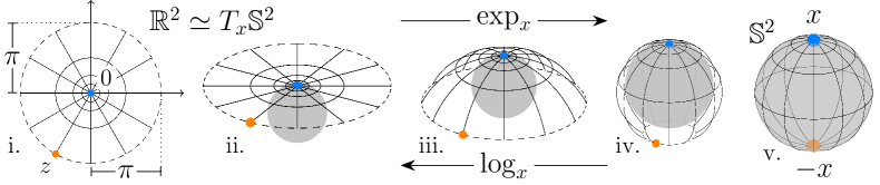
Figure 1: An illustration of the exponential map $\exp_{x}$ for the manifold $M=\mathbb{S}^{2}$, where $x$ is the “northpole” (blue) and $-x$ the “southpole” (orange). The logarithm map $\log_{x}$, discussed in Section 4.1, is a right-inverse to $\exp_{x}$, i.e., $\exp_{x}\circ\log_{x}$ is the identity. Panel i. The tangent space $T_{x}\mathbb{S}^{2}$ visualized as $\mathbb{R}^{2}$. The dashed circle encloses a disc of radius $\pi$. Panel ii. The tangent space realized as the hyperplane tangent to sphere at $x$. Panel iii-v. Animation showing $\exp_{x}$ as a bijection from the open disc of radius $\pi$ to $\mathbb{S}^{2}\setminus\{-x\}$. The entire dashed circle in Panel i is mapped to $-x$ the southpole. Thus, $\log_{x}$ maps the southpole $-x$ to a point $z$ on the dashed circle.

For a fixed $x\in M$, the above function $\exp_{x}$, the exponential map, can be defined on an open subset of $T_{x}M$ containing the origin. The Hopf-Rinow theorem ([20, Ch. 8, Theorem 2.8]) states that if $M$ is connected and complete with respect to the metric $\mathtt{dist}_{M}$, then $\exp_{x}$ can be defined on all of $T_{x}M$.

3 The Manifold-Hilbert kernel

Throughout the remainder of this work, we assume that $M$ is a complete, connected, and smooth Riemannian manifold of dimension $d$.

Definition 3.1.

We define the manifold-Hilbert kernel $K^{\mathcal{H}}_{M}:M\times M\to[0,\infty]$ for each $x,\xi\in M$ by $K^{\mathcal{H}}_{M}(x,\xi):=\mathtt{dist}_{M}(x,\xi)^{-d}$ if $x\neq\xi$ and $K^{\mathcal{H}}_{M}(x,x):=\infty$ otherwise.

Let $\lambda_{M}$ be the Riemann–Lebesgue volume measure of $M$. Integration with respect to this measure is denoted $\int_{M}fd\lambda_{M}$ for a function $f:M\to\mathbb{R}$. For details of the construction of $\lambda_{M}$, see [1, Proposition 1.5]. When $M=\mathbb{R}^{d}$, $\lambda_{M}$ is the ordinary Lebesgue measure and $\int_{\mathbb{R}^{d}}fd\lambda_{\mathbb{R}^{d}}$ is the ordinary Lebesgue integral. For this case, we simply write $\lambda$ instead of $\lambda_{\mathbb{R}^{d}}$.

We now state our first main result, a manifold theory extension of [19, Theorem 1].

Theorem 3.2.

Suppose that $X$ has a density $f_{X}$ with respect to $\lambda_{M}$ and that $Y$ is bounded. Let $P_{Y|X}$ be a conditional distribution of $Y$ given $X$ and $m_{Y|X}$ be its conditional expectation. Let $\widehat{m}_{n}(x):=\widehat{m}(x\|D^{n},K^{\mathcal{H}}_{M})$. Then

1. at almost all $x\in M$ with $f_{X}(x)>0$, we have $\widehat{m}_{n}(x)\to m_{Y|X}(x)$ in probability,

2. $J_{n}:=\int_{M}|\widehat{m}_{n}(x)-m_{Y|X}(x)|f_{X}(x)d\lambda_{M}(x)\to 0$ in probability.

In words, the kernel smoothing regression estimate $\widehat{m}_{n}$ based on the manifold-Hilbert kernel is consistent and interpolates the training data, provided $X$ has a density and $Y$ is bounded. As a consequence, following the same logic as in [19], the associated classifier $\mathtt{sgn}\circ\widehat{u}_{n}$ has the interpolating-consistent property. Before proving Theorem 3.2, we first review key concepts in probability theory on Riemannian manifolds.

3.1 Probability on Riemannian manifolds

Let $\mathcal{B}_{M}$ be the Borel $\sigma$-algebra of $M$, i.e., the smallest $\sigma$-algebra containing all open subsets of $M$. We recall the definition of $M$-valued random variables, following [32, Definition 2]:

Definition 3.3.

Let $(\Omega,\mathbb{P},\mathcal{A})$ be a probability space with measure $\mathbb{P}$ and $\sigma$-algebra $\mathcal{A}$. A $M$-valued random variable $X$ is a Borel-measurable function $\Omega\to M$, i.e., $X^{-1}(B)\in\mathcal{A}$ for all $B\in\mathcal{B}_{M}$.

Definition 3.4 (Density).

A random variable $X$ taking values in $M$ has a density if there exists a nonnegative Borel-measurable function $f:M\to[0,\infty]$ such that for all Borel sets $B$ in $M$, we have $\Pr(X\in B)=\int_{B}fd\lambda_{M}.$ The function $f$ is said to be a probability density function (PDF) of $X$.

Next, we recall the definition of conditional distributions, following [21, Ch. 10 §2]:

Definition 3.5 (Conditional distribution).

Let $(X,Y)$ be a random variable jointly distributed on $M\times\mathbb{R}$. Let $P_{X}(\cdot)$ be the probability measure corresponding to the marginal distribution of $X$. A conditional distribution for $Y$ given $X$ is a collection of probability measures $P_{Y|X}(\cdot|x)$ on $\mathbb{R}$ indexed by $x\in M$ satisfying the following:

1. For all Borel sets $A\subseteq\mathbb{R}$, the function $M\ni x\mapsto P_{Y|X}(A|x)\in[0,1]$ is Borel-measurable.

2. For all $A\subseteq\mathbb{R}$ and $B\subseteq M$ Borel sets, $\Pr(Y\in A,X\in B)=\int_{B}P_{Y|X}(A|x)P_{X}(dx)$.

The conditional expectation is defined as $m_{Y|X}(x):=\int_{\mathbb{R}}yP_{Y|X}(dy|x)$.

The existence of a conditional probability for a joint distribution $(X,Y)$ is guaranteed by [21, Theorem 10.2.2]. When $(X,Y)$ has a joint density $f_{XY}$ and marginal density $f_{X}$, the above definition gives the classical formula $P_{Y|X}(A|x)=\int_{A}f_{XY}(x,y)/f_{X}(x)dy$ when $\infty>f_{X}(x)>0$. See the first example in [21, Ch. 10 §2].

3.2 Lebesgue points on manifolds

[19] proved Theorem 3.2 when $M=\mathbb{R}^{d}$ and, moreover, that part 1 holds for the so-called Lebesgue points, whose definition we now recall.

Definition 3.6.

Let $f:M\to\mathbb{R}$ be an absolutely integrable function and $x\in M$. We say that $x$ is a Lebesgue point of $f$ if $f(x)=\lim_{r\to 0}\frac{1}{\lambda_{M}(\mathtt{B}_{x}(r,M))}\int_{\mathtt{B}_{x}(r,M)}fd\lambda_{M}$.

For an integrable function, the following result states that almost all points are its Lebesgue points. For the proof, see [24, Remark 2.4].

Theorem 3.7 (Lebesgue differentation).

Let $f:M\to\mathbb{R}$ be an absolutely integrable function. Then there exists a set $A\subseteq M$ such that $\lambda_{M}(A)=0$ and every $x\in M\setminus A$ is a Lebesgue point of $f$.

Next, for the reader’s convenience, we restate [19, Theorem 1], emphasizing the connection to Lebesgue points.

Theorem 3.8 ([19]).

Let $M=\mathbb{R}^{d}$ be the flat Euclidean space. Then Theorem 3.2 holds. Moreover, Part 1 holds for all $x$ that is a Lebesgue point to both $f_{X}$ and $m_{Y|X}\cdot f_{X}$.

The above result will be used in our proof of Theorem 3.2 below.

4 Proof of Theorem 3.2

The focal point of the first subsection is Lemma 4.1 which shows the Borel measurability of extensions of the so-called Riemannian logarithm. The second subsection contains two key results regarding densities of $M$-valued random variables transformed by the Riemannian logarithm. The final subsection proves Theorem 3.2 leveraging results from the preceding two subsections.

4.1 The Riemannian logarithm

Throughout, $x$ is assumed to be an arbitrary point of $M$. Let $U_{x}M=\{v\in T_{x}M:\|v\|_{x}=1\}\subseteq T_{x}M$ denote the set of unit tangent vectors. Define a function $\tau_{x}:U_{x}M\to(0,\infty]$ as follows:

$$\tau_{x}(u):=\sup\{t>0:t=\mathtt{dist}_{M}(x,\exp_{x}(tu))\}.$$

The tangent cut locus is the set $\tilde{C}_{x}\subseteq T_{x}M$ defined by $\tilde{C}_{x}:=\{\tau_{x}(u)u:u\in U_{x}M,\,\tau_{x}(u)<\infty\}.$ Note that it is possible for $\tau_{x}(u)=\infty$ for all $u\in U_{x}M$ in which case $\tilde{C}_{x}$ is empty. The cut locus is the set $C_{x}:=\exp_{x}(\tilde{C}_{x})\subseteq M$.

The tangent interior set is $\tilde{I}_{x}:=\{tu:0\leq t<\tau_{x}(u),u\in U_{x}M\}$ and the interior set is the set $I_{x}:=\exp_{x}(\tilde{I}_{x})$. Finally, define $\tilde{D}_{x}:=\tilde{I}_{x}\cup\tilde{C}_{x}$. Note that for each $z=tu\in\tilde{I}_{x}$, we have

$$\|z\|_{x}=t=\mathtt{dist}_{M}(x,\exp_{x}(tu))=\mathtt{dist}_{M}(x,\exp_{x}(z)).$$ (6)

Consider the example where $M=\mathbb{S}^{2}$ as in Figure 1. Then $\tau_{x}(u)=\pi$ for all $u\in U_{x}M$. Thus, the tangent interior set $\tilde{I}_{x}=\mathtt{B}_{0}(\pi,\mathbb{R}^{2})$, the open disc of radius $\pi$ centered at the origin.

When restricted to $\tilde{I}_{x}$, the exponential map $\exp_{x}|_{\tilde{I}_{x}}:\tilde{I}_{x}\to I_{x}$ is a diffeomorphism. Its functional inverse, denoted by $\log_{x}|_{I_{x}}$, is called the Riemannian Logarithm [8, 43]. In previous works, $\log_{x}|_{I_{x}}$ is only defined from $I_{x}$ to $\tilde{I}_{x}$. The next result shows that the domain of $\log_{x}|_{I_{x}}:I_{x}\to\tilde{I}_{x}$ can be extended to $\log_{x}:M\to\tilde{D}_{x}$ while remaining Borel-measurable.

Lemma 4.1.

For all $x\in M$, there exists a Borel measurable map $\log_{x}:M\to T_{x}M$ such that $\log_{x}(M)\subseteq\tilde{{D}}_{x}$ and $\exp_{x}\circ\log_{x}$ is the identity on $M$. Furthermore, for all $x,\xi\in M$, we have $\mathtt{dist}_{M}(x,\xi)=\|\log_{x}(\xi)\|_{x}$.

Proof sketch.

The full proof of the lemma is provided in Section A.2 of the Appendix. Below, we illustrate the idea of the proof using the example when $M=\mathbb{S}^{2}$ as in Figure 1.

Let $x\in\mathbb{S}^{2}$ be the “northpole” (the blue point). The tangent cut locus $\tilde{C}_{x}$ is the dashed circle in the left panel of Figure 1. The exponential map $\exp_{x}$ is one-to-one on $\tilde{D}_{x}$ except on the dashed circle, which all gets mapped to $-x$, the “southpole” (the orange point). A consequence of the measurable selection theorem is that $\log_{x}$ can be extended to be a Borel-measurable right inverse of $\exp_{x}$ by selecting $z$ point on $\tilde{C}_{x}$ such that $\log_{x}(-x)=z$. ∎

4.2 Random variable transforms

In the previous subsection, we showed that $\log_{x}:M\to T_{x}M$ is Borel-measurable. Now, recall that $T_{x}M$ is equipped with the inner product $\langle\cdot,\cdot\rangle_{x}$, i.e., the Riemannian metric. Below, for each $x\in M$ choose an orthonormal basis on $T_{x}M$ with respect to $\langle\cdot,\cdot\rangle$. Then $T_{x}M$ is isomorphic as an inner product space to $\mathbb{R}^{d}$ with the usual dot product.

Our first result of this subsection is a “change-of-variables formula” for computing the densities of $M$-valued random variables after the $\log_{x}$ transform. Recall that $\lambda_{M}$ is the Riemann-Lebesgue measure on $M$ and $\lambda$ is the ordinary Lebesgue measure on $\mathbb{R}^{d}=T_{x}M$.

Proposition 4.2.

Let $x\in M$ be fixed. There exists a Borel measurable function $\nu_{x}:M\to\mathbb{R}$ with the following properties:

1. Let $X$ be a random variable on $M$ with density $f_{X}$ and let $Z:=\log_{x}(X)$. Then $Z$ is a random variable on $T_{x}M$ with density $f_{Z}(z):=f_{X}(\exp_{x}(z))\cdot\nu_{x}(\exp_{x}(z))$.

2. Let $f:M\to\mathbb{R}$ be an absolutely integrable function such that $x$ is a Lebesgue point of $f$. Define $f:T_{x}M\to\mathbb{R}$ by $h(z):=f(\exp_{x}(z))\cdot\nu_{x}(\exp_{x}(z))$. Then $0\in T_{x}M$ is a Lebesgue point for $h$.

Proof sketch.

The full proof of the proposition is in Appendix Section A.3. The function $\nu_{x}$ is the Jacobian of the change-of-variables formula for integrating $\int_{\tilde{B}}f_{Z}d\lambda$ where $\tilde{B}\subseteq T_{x}M$ is a Borel subset. See Appendix Lemma A.4 for the exact definition of $\nu_{x}$. Part (i) is a simple consequence of this change-of-variables formula, which says that $\int_{\tilde{B}}f_{Z}d\lambda=\int_{\exp_{x}(\tilde{B})}hd\lambda_{M}$.

For part (ii), the key observations are that (a) $\nu_{x}(\exp_{x}(0))=\nu_{x}(0)=1$ and (b) the volumes of $\mathtt{B}_{x}(r,M)$ and $\mathtt{B}_{0}(r,T_{x}M)$ are equal as $r\to 0$. More precisely, $\lim_{r\to 0}\frac{\lambda_{M}(\mathtt{B}_{x}(r,M))}{\lambda(\mathtt{B}_{0}(r,T_{x}M))}=1$. From these two observations, it is straightforward to directly verify Definition 3.6. ∎

Proposition 4.3.

Let $(X,Y)$ have a joint distribution on $M\times\mathbb{R}$ such that the marginal of $X$ has a density $f_{X}$ on $M$. Let $P_{Y|X}(\cdot|\cdot)$ be a conditional distribution for $Y$ given $X$. Let $x\in M$. Define $Z:=\log_{x}(X)$ and consider the joint distribution $(Z,Y)$ on $T_{p}M\times\mathbb{R}$. Then $P_{Y|Z}(\cdot|\cdot):=P_{Y|X}(\cdot|\exp_{x}(\cdot))$ is a conditional distribution for $Y$ given $Z$. Consequently, $m_{Y|X}\circ\exp_{x}=m_{Y|Z}$.

Proof sketch.

The full proof of the Proposition is in Appendix Section A.4. The idea is the same as in the proof of Proposition 4.2, except that the probability density $f_{Z}$ is replaced by an appropriate conditional probability density. ∎

4.3 Finishing up the Proof of Theorem 3.2

Fix $x\in M$ such that $x$ is a Lebesgue point of $f_{X}$ and $m_{Y|X}\cdot f_{X}$. Note that by Theorem 3.7, almost all $x\in M$ has this property. Next, let $Z=\log_{x}(X)$ and $f_{Z}$ be as in Proposition 4.2-(i). Then

1. $f_{Z}=(f_{X}\circ\exp_{x})\cdot(\nu_{x}\circ\exp_{x})$, and

2. $(m_{Y|X}\circ\exp_{x})\cdot f_{Z}=(m_{Y|X}\circ\exp_{x})\cdot(f_{X}\circ\exp_{x})\cdot(\nu_{x}\circ\exp_{x})$.

Now, proposition 4.2-(ii) implies that $0$ is a Lebesgue point of both $f_{Z}$ and $(m_{Y|X}\circ\exp_{x})\cdot f_{Z}$. Furthermore, by Proposition 4.3, we have $m_{Y|X}\circ\exp_{x}=m_{Y|Z}$. Thus, $0$ is a Lebesgue point of $f_{Z}$ and $m_{Y|Z}\cdot f_{Z}$.

Now, let $D_{n}:=\{(X_{i},Y_{i})\}_{i\in[n]}$. Define $Z_{i}:=\log_{x}(X_{i})$, which are i.i.d copies of the random variable $Z:=\log_{x}(X)$, and let $\tilde{D}_{n}:=\{(Z_{i},Y_{i})\}_{i\in[n]}$. Then we have

$$\widehat{m}(x\|D^{n},K^{\mathcal{H}}_{M}) \overset{\mathrm{(a)}}{=}\frac{\sum_{i=1}^{n}Y_{i}\cdot\mathtt{dist}_{M}(x,X_{i})^{-d}}{\sum_{j=1}^{n}\mathtt{dist}_{M}(x,X_{j})^{-d}}\overset{\mathrm{(b)}}{=}\frac{\sum_{i=1}^{n}Y_{i}\cdot\|Z_{i}\|_{x}^{-d}}{\sum_{j=1}^{n}\|Z_{j}\|_{x}^{-d}}$$

$$\overset{\mathrm{(c)}}{=}\frac{\sum_{i=1}^{n}Y_{i}\cdot\mathtt{dist}_{\mathbb{R}^{d}}(0,Z_{i})^{-d}}{\sum_{j=1}^{n}\mathtt{dist}_{\mathbb{R}^{d}}(0,Z_{j})^{-d}}\overset{\mathrm{(d)}}{=}\widehat{m}(0\|\tilde{D}^{n},K^{\mathcal{H}}_{\mathbb{R}^{d}})$$

where equations marked by (a) and (d) follow from Equation (5), (b) from Lemma 4.1, and (c) from the fact that the inner product space $T_{x}M$ with $\langle\cdot,\cdot\rangle_{x}$ is isomorphic to $\mathbb{R}^{d}$ with the usual dot product. By Theorem 3.8, we have $\widehat{m}(0\|\tilde{D}^{n},K^{\mathcal{H}}_{\mathbb{R}^{d}})\to m_{Y|Z}(0)$ in probability. In other words, for all $\epsilon>0$,

$$\lim_{n\to\infty}\Pr\{|\widehat{m}(0\|\tilde{D}^{n},K^{\mathcal{H}}_{\mathbb{R}^{d}})-m_{Y|Z}(0)|>\epsilon\}=0.$$

By Proposition 4.3, we have $m_{Y|Z}(0)=m_{Y|Z}(\exp_{x}(0))=m_{Y|Z}(x)$. Therefore,

$$\Big{\{}|\widehat{m}(0\|\tilde{D}^{n},K^{\mathcal{H}}_{\mathbb{R}^{d}})-m_{Y|Z}(0)|>\epsilon\Big{\}}=\Big{\{}|\widehat{m}(x\|D^{n},K^{\mathcal{H}}_{M})-m_{Y|X}(x)|>\epsilon\Big{\}}$$

as events. Thus, $\widehat{m}(x\|D^{n},K^{\mathcal{H}}_{M})\to m_{Y|X}(x)$ converges in probability, proving Theorem 3.2 part 1. As noted in [19, §2], part 2 of Theorem 3.2 is an immediate consequence of part 1.

5 Application to the $d$-Sphere

The $d$-dimensional round sphere is $\mathbb{S}^{d}:=\{x\in\mathbb{R}^{d+1}:x^{2}_{1}+\cdots+x^{2}_{d+1}=1\}$. Here, a round sphere assumes that $\mathbb{S}^{d}$ has the arc-length metric:

$$\mathtt{dist}_{\mathbb{S}^{d}}(x,z)=\angle(x,z)=\cos^{-1}(x^{\top}z)\in[0,\pi].$$ (7)

Let $\mathcal{S}$ be a set and $\sigma:M\to\mathcal{S}$ be a function. The partition induced by $\sigma$ is defined by $\{\sigma^{-1}(s):s\in\mathtt{Range}(\sigma)\}$. For example, when $M=\mathbb{S}^{d}$ and $W\in\mathbb{R}^{(d+1)\times h}$, then the function $\sigma_{W}:\mathbb{S}^{d}\to\{\pm 1\}^{h}$ defined by $\sigma_{W}(x)=\mathtt{sgn}(W^{\top}x)$ induces a hyperplane arrangement partition.

Let $\mathbb{N}=\{1,2,\dots\}$ and $\mathbb{N}_{0}=\mathbb{N}\cup\{0\}$ denote the positive and non-negative integers.

Definition 5.1 (Random hyperplane arrangement partition).

Let $d\in\mathbb{N}$ and $M=\mathbb{S}^{d}$. Let $q<0$ be a negative number, and let $H$ be a random variable with probability mass function $p_{H}:\mathbb{N}_{0}\to[0,1]$ such that $p_{H}(h)>0$ for all $h$. Define the following weighted random partition ${\mathsf{ha}}:=(\Theta,\mathfrak{P},\alpha)$:

1. The parameter space $\Theta=\bigsqcup_{h=0}^{\infty}\mathbb{R}^{(d+1)\times h}$ is the disjoint union of all $(d+1)\times h$ matrices. Element of $\Theta$ are matrices $\theta=W\in\mathbb{R}^{(d+1)\times h}$ where the number of columns $h\in\{0,1,2,\dots\}$ varies. By convention, if $h=0$, the partition $\mathcal{P}_{\theta}=\mathcal{P}_{W}$ is the trivial partition $\{\mathbb{S}^{d}\}$. If $h>0$, $\mathcal{P}_{W}$ is the partition induced by $x\mapsto\mathtt{sgn}(W^{\top}x)$.

2. The probability $\mathfrak{P}$ is constructed by the procedure where we first sample $h\sim p_{H}(h)$, then sample the entries of $W\in\mathbb{R}^{d\times h}$ i.i.d according to $\mathtt{Gaussian}(0,1)$.

3. For $\theta\in\Theta$, define $\alpha(\theta):=\pi^{q}p_{H}(h)^{-1}(-1)^{h}\binom{q}{h}$, where $\binom{q}{h}:=\tfrac{1}{h!}\prod_{j=0}^{h-1}(q-j)$.

Note that $(-1)^{h}\binom{q}{h}=\tfrac{1}{h!}\prod_{j=0}^{h-1}(q-j)>0$ when $q<0$.

Theorem 5.2.

Let ${\mathsf{ha}}=(\Theta,\mathfrak{P},\alpha)$ be as in Definition 5.1. Then

$$K^{\mathsf{ha}}_{\mathbb{S}^{d}}(x,z)=\begin{cases}\angle(x,z)^{q}&:\angle(x,z)\neq 0\\ +\infty&:\mbox{otherwise.}\end{cases}$$

When $q=-d$, we have $K^{\mathsf{ha}}_{\mathbb{S}^{d}}=K^{\mathcal{H}}_{\mathbb{S}^{d}}$ where the right hand side is the manifold-Hilbert kernel.

Proof of Theorem 5.2.

Before proceeding, we have the following useful lemma:

Lemma 5.3.

Let ${\mathsf{rp}}=(\Theta,\mathfrak{P},\alpha)$ be a WRP. Let $H$ be a random variable. Let $\theta\sim\mathfrak{P}$. Suppose that for all $x,z\in M$, the random variables $\alpha(\theta)$ and $\mathbb{I}\{x\in\mathcal{P}_{\theta}[z]\}$ are conditionally independent given $H$. Then we have $K^{\mathsf{rp}}_{M}(x,z)=\mathbb{E}_{H}\Big{[}\overline{\alpha}(H)\cdot\mathbb{E}_{\theta\sim\mathfrak{P}}[\mathbb{I}\{x\in\mathcal{P}_{\theta}[z]\}|H]\Big{]}$ where $\overline{\alpha}(h):=\mathbb{E}_{\theta\in\mathfrak{P}}\left[\alpha(\theta)|H=h\right]$ for a realization $h$ of $H$.

The lemma follows immediately from the Definition of $K^{\mathsf{rp}}_{M}(x,z)$ in Equation 3 and the conditional independence assumption. Now, we proceed with the proof of Theorem 5.2.

Let $\phi:=\angle(x,z)/\pi$. Let $H\sim p_{H}$ and $\theta\sim\mathfrak{P}$ be the random variables in Definition 5.1. Note that by construction, the following condition is satisfied: for all $x,z\in M$, the random variables $\alpha(\theta)$ and $\mathbb{I}\{x\in\mathcal{P}_{\theta}[z]\}$ are conditionally independent given $H$. In fact, $\alpha(\theta)=\pi^{q}p_{H}(h)^{-1}(-1)^{h}\binom{q}{h}$ is constant given $H=h$. Hence, applying Lemma 5.3, we have

$$K^{\mathsf{ha}}_{\mathbb{S}^{d}}(x,z)=\mathbb{E}_{H}\Big{[}\overline{\alpha}(H)\cdot\mathbb{E}_{\theta\sim\mathfrak{P}}[\mathbb{I}\{x\in\mathcal{P}_{\theta}[z]\}|H]\Big{]}$$

$$=\sum_{h=0}^{\infty}\pi^{q}(-1)^{h}\binom{q}{h}\cdot\mathbb{E}_{\theta\sim\mathfrak{P}}[\mathbb{I}\{x\in\mathcal{P}_{\theta}[z]\}|H=h]=\sum_{h=0}^{\infty}\pi^{q}(-1)^{h}\binom{q}{h}\cdot\Pr\{x\in\mathcal{P}_{\theta}[z]|H=h\}.$$

Next, we claim that $\Pr\{x\in\mathcal{P}_{\theta}[z]|H=h\}=(1-\phi)^{h}.$ When $h=0$, $x\in\mathcal{P}_{\theta}[z]$ is always true since $\mathcal{P}_{\theta}=\{\mathbb{S}^{d}\}$ is the trivial partition. In this case, we have $\Pr\{x\in\mathcal{P}_{\theta}[z]|H=h\}=1=(1-\phi)^{0}$. When $h>0$, we recall a result of [33]:

Lemma 5.4.

Let $x,z\in\mathbb{S}^{d}$. Let $w\in\mathbb{R}^{d+1}$ be a random vector whose entries are sampled i.i.d according to $\mathtt{Gaussian}(0,1)$. Then $\Pr\{\mathtt{sgn}(w^{\top}x)=\mathtt{sgn}(w^{\top}z)\}=1-(\angle(x,z)/\pi)$.

Let $W=[w_{1},\dots,w_{h}]$ be as in Definition 5.1 where $w_{j}$ denotes the $j$-th column of $W$. Then by construction, $w_{j}$ is distributed identically as $w$ in Lemma 5.4. Furthermore, $w_{j}$ and $w_{j^{\prime}}$ are independent for $j,j^{\prime}\in[h]$ where $j\neq j^{\prime}$. Thus, the claim follows from

$$\Pr\{x\in\mathcal{P}_{\theta}[z]|H=h\} \overset{\mathrm{(a)}}{=}\Pr\{\mathtt{sgn}(W^{\top}x)=\mathtt{sgn}(W^{\top}z)|H=h\}$$

$$\overset{\mathrm{(b)}}{=}\prod_{j=1}^{h}\Pr\{\mathtt{sgn}(w_{j}^{\top}x)=\mathtt{sgn}(w_{j}^{\top}z)\}\overset{\mathrm{(c)}}{=}\prod_{j=1}^{h}\left(1-\phi\right)=\left(1-\phi\right)^{h}.$$

where equality (a) follows from Definition 5.1, (b) from $W\in\mathbb{R}^{(d+1)\times h}$ having i.i.d standard Gaussian entries given $H=h$, and (c) from Lemma 5.4. Putting it all together, we have

$$K^{\mathtt{part}}_{\mathfrak{P},\alpha}(x,z)=\sum_{h=0}^{\infty}\pi^{q}(-1)^{h}\binom{q}{h}(1-\phi)^{h}=\pi^{q}\sum_{h=0}^{\infty}\binom{q}{h}(\phi-1)^{h}=\angle(x,z)^{q}.$$

For the last step, we used the fact that for all $q\in\mathbb{R}$ the binomial series $(1+t)^{q}=\sum_{h=0}^{\infty}\binom{q}{h}t^{h}$ converges absolutely for $|t|<1$ (when $\phi\in(0,1]$) and diverges to $+\infty$ for $t=-1$ (when $\phi=0$). ∎

Corollary 5.5.

Let $q:=-d$ and $K^{\mathsf{ha}}_{\mathbb{S}^{d}}$ be as in Theorem 5.2. The infinite-ensemble classifier $\mathtt{sgn}(\widehat{u}(\bullet\|D^{n},K^{\mathsf{ha}}_{\mathbb{S}^{d}}))$ (see Equation 4 for definition) has the interpolating-consistent property.

Proof.

As observed in [19, Section 7], for an arbitrary kernel $K$, the $L_{1}$-consistency of $\widehat{m}(\bullet\|D^{n},K)$ for regression implies the consistency for classification of $\mathtt{sgn}(\widehat{u}(\bullet\|D^{n},K))$. Furthermore, $\widehat{m}(\bullet\|D^{n},K)$ is interpolating for regression implies that $\mathtt{sgn}(\widehat{u}(\bullet\|D^{n},K))$ is interpolating for classification. While the argument there is presented in the $\mathbb{R}^{d}$ case, the argument holds in the more general manifold case mutatis mutandis.

Thus, by Theorem 3.2, we have $\mathtt{sgn}(\widehat{u}(\bullet\|D^{n},K^{\mathcal{H}}_{\mathbb{S}^{d}}))$ is consistent for classification, i.e., Equation (1) holds. It is also interpolating since $\widehat{m}(\bullet\|D^{n},K)$ is interpolating. By Proposition 5.2, we have $K^{\mathsf{ha}}_{\mathbb{S}^{d}}=K^{\mathcal{H}}_{\mathbb{S}^{d}}$. Thus $\mathtt{sgn}(\widehat{u}(\bullet\|D^{n},K^{\mathsf{ha}}_{\mathbb{S}^{d}}))$ is an ensemble method having the interpolating-consistent property. ∎

6 Discussion

We have shown that using the manifold-Hilbert kernel in kernel smoothing regression, also known as Nadaraya-Watson regression, results in a consistent estimator that interpolates the training data on a Riemannian manifold $M$. Furthermore, when $M=\mathbb{S}^{d}$ is the sphere, we showed that the manifold-Hilbert kernel is a weighted random partition kernel, where the random partitions are induced by random hyperplane arrangements. This demonstrates an ensemble method that has the interpolating-consistent property.

A limitation of this work is that the random hyperplane arrangement partition is data-independent. Thus, the resulting ensemble method considered in this work are easier to analyze than popular ensemble methods used in practice. Nevertheless, we believe our work offers one theoretical basis towards understanding generalization in the interpolation regime of ensembles of histogram classifiers over data-dependent partitions, e.g., decision trees à la CART [15].

A.1 Basics of Riemannian Manifolds

In this section, we review the main concepts from Riemannian manifold theory essential to this work. Our main references are [34] and [20]. Throughout, $d\in\mathbb{N}$ denotes the dimension. We use the word smooth to mean infinitely differentiable.

Manifolds. A smooth manifold $M$ of dimension $d$ is a Hausdorff, second countable topological space together with an atlas: a set $\mathtt{Atlas}:=\{(U_{\alpha},\varphi_{\alpha})\}_{\alpha\in A}$ where 1). $\{U_{\alpha}\}_{\alpha\in A}$ is an open cover of $M$, 2). for each $\alpha\in A$, $\varphi_{\alpha}:U_{\alpha}\to\varphi_{\alpha}(U_{\alpha})\subseteq\mathbb{R}^{d}$ is a homeomorphism onto its image, and 3). $\varphi_{\alpha}\circ\varphi_{\beta}^{-1}:\varphi_{\beta}(U_{\alpha}\cap U_{\beta})\to\varphi_{\alpha}^{-1}(U_{\alpha}\cap U_{\beta})$ is smooth for each pair $\alpha,\beta\in A$. An element $(U,\varphi)$ of $\mathtt{Atlas}$ is called a chart.

Smooth maps. A real-valued function $f:M\to\mathbb{R}$ is a smooth function if $f\circ\varphi^{-1}$ is smooth (in the elementary calculus sense) for all charts $(U,\varphi)$. The set of all smooth functions is denoted $\mathtt{Fn}(M)$, which forms an $\mathbb{R}$-vectorspace. Let $N$ be another smooth manifold with atlas $\mathcal{B}$. A function $\Phi:M\to N$ is a smooth map if $g\circ\Phi\in\mathtt{Fn}(M)$ for all $g\in\mathtt{Fn}(N)$.

Tangent space. Let $x\in M$. A derivation at $x$ is a linear function $v:\mathtt{Fn}(M)\to\mathbb{R}$ satisfying the product rule: $v[fg]=f(x)v[f]+g(x)v[g]$ for all $f,g\in\mathtt{Fn}(M)$. The tangent space at $x$, denoted $T_{x}M$, is the vector space of all derivations at $x$. Elements of $T_{x}M$ are referred to as tangent vectors at $x$. For a given chart $(U,\varphi)$ where $x\in U$, define a derivation at $x$, denoted $\partial_{i}|_{x}$, by $f\mapsto\frac{d(f\circ\varphi^{-1})}{dz_{i}}(\varphi(x))$ where $\frac{d}{dz_{i}}$ is the $i$-th partial derivative in ordinary calculus. It is a fact that $\{\partial_{i}|_{x}:i=1,\dots,d\}$ is a basis for $T_{x}M$.

Although the above definition of a tangent vector is abstract, it can be concretely interpreted in terms of derivative along a curve. Let $a<t_{0}<b$ be real numbers. A curve through $x$ is a smooth map $\gamma:(a,b)\to M$ such that $\gamma(t_{0})=x$. Then $\mathtt{Fn}(M)\ni f\mapsto\frac{d}{dt}f(\gamma(t))|_{t=t_{0}}\in\mathbb{R}$ defines a derivation at $x$. Oftentimes, this derivation is denoted $\dot{\gamma}(t_{0})\in T_{x}M$

Riemannian metric. The tangent bundle is the set $TM:=\bigcup_{x}T_{x}M$, which itself is a smooth manifold of dimension $2d$. A vector field on $M$ is a smooth map $\mathsf{V}:M\to TM$ such that $\mathsf{V}(x)\in T_{x}M$ for all $x\in M$. The set of all vectors fields on $M$ is denoted $\mathtt{Vf}(M)$.

A Riemannian metric on $M$ is a choice of an inner product $\langle\cdot,\cdot\rangle_{x}$ (and thus, a norm $\|\cdot\|_{x}$) on $T_{x}M$ for each $x\in M$ such that the function $M\to\mathbb{R}$ given by $x\mapsto\langle\mathsf{V}(x),\mathsf{U}(x)\rangle_{x}$ is smooth for all $\mathsf{V},\mathsf{U}\in\mathtt{Vf}(M)$. As shorthands, when $x$ is clear from context, we drop the subscripts and simply write $\langle\cdot,\cdot\rangle$ and $\|\cdot\|$ instead. Choosing an orthonormal basis for $T_{x}M$ with respect to $\langle\cdot,\cdot\rangle_{x}$ for each $x$, we can identify $T_{x}M$ with $\mathbb{R}^{d}$ with the ordinary dot inner product.

Let $x\in M$ and $(U,\varphi)$ be a chart such that $x\in U$. Define $g_{ij}(x)=\langle\partial_{i}|_{x},\partial_{j}|_{x}\rangle_{x}$. Denote by $G(x)$ the $d\times d$ positive definite matrix $[g_{ij}(x)]_{ij}$. Below, we will refer to the function $G:U\to\mathbb{R}^{d\times d}$ as the coordinate representation of the Riemannian metric. Define $g^{ij}(x):=[G(x)^{-1}]_{ij}$. The Christoffel symbols with respect to $(U,\varphi)$ are defined by $\Gamma^{k}_{ij}:=\frac{1}{2}\sum_{\ell=1}^{d}g^{k\ell}(\partial_{i}|_{x}g_{j\ell}+\partial_{j}|_{x}g_{i\ell}-\partial_{\ell}|_{x}g_{ij})$. Note that $g_{k\ell}$, $g^{k\ell}$, $G$, $\Gamma^{k}_{ij}$, and $\partial_{i}|_{x}g_{j\ell}$ are all functions with domain $U$.

Geodesics. Fix a chart $(U,\varphi)$. Consider a smooth curve $\gamma:[a,b]\to U$. Let $\zeta_{i}(t):=[\varphi(\gamma(t))]_{i}$ be the $i$-th component functions. The curve $\gamma$ is a geodesic if $\zeta$ is a solution to the following system of second order ordinary differential equations (ODEs): $\frac{d^{2}\zeta_{i}}{dt^{2}}+\sum_{j,\ell=1}^{d}\Gamma^{i}_{j\ell}\circ\gamma\frac{d\zeta_{j}}{dt}\frac{d\zeta_{\ell}}{dt}=0$ for all $i=1,\dots,d$ at all time $t\in[a,b]$.

Geodesics are minimizers of the so-called energy functional $E(\gamma)=\frac{1}{2}\int_{a}^{b}\|\dot{\gamma}(t)\|_{\gamma(t)}^{2}dt$. The above system of ODEs are the analog of the “first derivative test” for local minimizers of $E$. Thus, geodesics are defined independently of the choice of the chart.

Exponential map. For $x\in M$ and $v\in T_{x}M$, there exists $\epsilon>0$ and a unique geodesic curve $\gamma_{v}:[-\epsilon,\epsilon]\to M$ such that $\gamma_{v}(0)=x$ and $\dot{\gamma}_{v}(0)=v$. This follows from the existence and uniqueness of the solution to an ODE given initial conditions where the ODE is as discussed above. Note that although geodesics are previously defined in $U$ where $(U,\varphi)$ is a chart, they can be extended outside of $U$ using additional charts.

Let $x\in M$ and $v\in T_{x}M$ be fixed and let $\gamma_{v}:[-\epsilon,\epsilon]\to M$ be as in the preceding paragraph. If $\|v\|_{x}\leq\epsilon$, then define $\exp_{x}(v):=\gamma_{v}(1)$. A fundamental fact is that $\exp_{x}$, known as the exponential map at $x$, can be defined on an open set of $T_{x}M$ containing the origin.

Distance function. Let $x,\xi\in M$ and $a<b$ be real numbers. A piecewise smooth curve from $x$ to $\xi$ is a piecewise smooth map $\gamma:[a,b]\to M$ such that $\gamma(a)=x$ and $\gamma(b)=\xi$. Assume that $M$ is connected. Then for all $x,\xi\in M$, there exists a piecewise smooth curve from $x$ to $\xi$. The length of $\gamma$ is defined as $\mathtt{len}(\gamma):=\int_{a}^{b}\|\dot{\gamma}(t)\|_{\gamma(t)}dt$. Define $\mathtt{dist}_{M}(x,\xi):=\inf\{\mathtt{len}(\gamma):\gamma$ is a piecewise smooth curve from $x$ to $\xi\}$, which is a metric on $M$ in the sense of metric spaces (see [34, Proposition 1.1]). For $x\in M$ and $r\in(0,\infty)$, the open ball centered at $x$ of radius $r$ is denoted $\mathtt{B}_{x}(r,M):=\{z\in M:\mathtt{dist}_{M}(x,z)<r\}$.

Complete Riemannian manifolds. A Riemannian manifold is complete if it is a complete metric space under the metric $\mathtt{dist}_{M}$. The Hopf-Rinow theorem ([20, Ch. 8, Theorem 2.8]) states that if $M$ is connected and complete, then the exponential $\exp_{x}$ can be defined on the entire $T_{x}M$.

A.2 Proof of Lemma 4.1

This section uses definitions and notations introduced in Section 4.1. In particular, recall the cut locus $C_{x}$, the tangent cut locus $\tilde{C}_{x}$, the interior set $I_{x}$ and the tangent interior set $\tilde{I}_{x}$. The proof of Lemma 4.1 is presented towards the end of the section. At this point, we compile some facts from various sources about the cut locus.

Lemma A.1.

For all $x\in M$, we have

1. $C_{x}$ is a closed subset of $M$ ([26, Proposition 1.2]).

2. $I_{x}\cap C_{x}=\emptyset$ and $I_{x}\cup C_{x}=M$ ([34, Ch II, Lemma 4.4 (1)])

3. $I_{x}$ is an open subset of $M$ (immediate from 1 and 2 above)

4. $\exp_{x}:\tilde{I}_{x}\to I_{x}$ is a diffeomorphism ([34, Ch II, Lemma 4.4 (2)])

5. $\lambda_{M}(C_{x})=0$, where $\lambda_{M}$ is the Riemann-Lebesgue measure ([34, Lemma 4.4 (3)])

6. $\tau_{x}$ is continuous and $\inf_{u\in U_{x}M}\tau_{x}(u)>0$ ([34, Ch II, Propositions 4.1 (2) and 4.13 (1)])

While the following lemma is elementary, we provide a proof since we could not find one in the literature.

Lemma A.2.

For all $x\in M$, the (topological) closure of $\tilde{I}_{x}$ in $T_{x}M$ is $\tilde{D}_{x}$. Furthermore, for all $x\in M$, we have $\exp_{x}(\tilde{D}_{x})=M$.

Proof of Lemma A.2.

Take a convergent sequence $\{t_{i}u_{i}\}_{i\in\mathbb{N}}\subseteq\tilde{I}_{x}$ where $u_{i}\in U_{x}M$ and $0\leq t_{i}<\tau_{x}(u_{i})$. Let $v^{*}=\lim_{i}t_{i}u_{i}$. Our goal is to show that $v^{*}\in\tilde{D}_{x}=\tilde{I}_{x}\cup\tilde{C}_{x}$.

Since $U_{x}M$ is compact, we may assume that $u^{*}:=\lim_{i}u_{i}$ exists after passing to a subsequence if necessary. Furthermore, $\|t_{i}u_{i}\|_{x}=t_{i}$ implies that $t^{*}:=\lim_{i}t_{i}$ exists as well (i.e., $t^{*}<\infty$). Hence, $v^{*}=t^{*}u^{*}$.

Consider the case that $\tau_{x}(u^{*})=\infty$. Then $0\leq t^{*}<\tau_{x}(u^{*})$ implies that $v^{*}=t^{*}u^{*}\in\tilde{I}_{x}$. For the other case that $t(u)<\infty$, we first note that $t_{i}u_{i}\in\tilde{I}_{x}$ implies that $t_{i}<\tau_{x}(u_{i})$. Taking the limit of both sides, we have $t^{*}=\lim_{i}t_{i}\leq\lim_{i}\tau_{x}(u_{i})=\tau_{x}(u^{*}).$ Note that the last limit can be exchanged since $\tau_{x}$ is continuous (Lemma A.1 part 6). Thus, either $t^{*}<\tau_{x}(u^{*})$ in which case $v^{*}\in\tilde{I}_{x}$, or $t^{*}=\tau_{x}(u^{*})$ in which case $v^{*}=\tau_{x}(u^{*})u^{*}\in\tilde{C}_{x}$.

For the “furthermore” part, note that

$$\exp_{x}(\tilde{D}_{x})=\exp_{x}(\tilde{I}_{x}\cup\tilde{C}_{x})=\exp_{x}(\tilde{I}_{x})\cup\exp_{x}(\tilde{C}_{x})={I}_{x}\cup{C}_{x}=M$$

where the last equality is Lemma A.1 part 2. ∎

Proof of Lemma 4.1.

Denote by $\mathrm{cl}(T_{x}M)$ the set of closed subsets of $T_{x}M$. Define $\psi:M\to\mathrm{cl}(T_{x}M)$ by $\psi(\xi):=\{x\in\tilde{D}_{x}:\exp_{x}(x)=\xi\}=\exp_{x}^{-1}(\xi)\cap\tilde{D}_{x}.$ Note that $\psi(\xi)$ is a closed set by Lemma A.2.

We claim that $\psi$ is weakly-measurable, i.e., for every open set $\tilde{U}\subseteq T_{x}M$, the subset of $M$ defined by $\{\xi\in M:\psi(\xi)\cap\tilde{U}\neq\emptyset\}$ is Borel. To see this, note that

$$\{\xi\in M:\psi(\xi)\cap\tilde{U}\neq\emptyset\}$$

$$=\{\xi\in M:\exp_{x}^{-1}(\xi)\cap\tilde{D}_{x}\cap\tilde{U}\neq\emptyset\}$$

$$=\{\xi\in M:\exp_{x}(\tilde{D}_{x}\cap\tilde{U})\ni\xi\}$$

$$=\exp_{x}(\tilde{D}_{x}\cap\tilde{U}).$$

As inner product spaces, $T_{x}M$ and $\mathbb{R}^{d}$ are isomorphic (see Section A.1-Riemannian metric). Since, $T_{x}M$ and $\mathbb{R}^{d}$ are homeomorphic as topological spaces, $\mathbb{R}^{d}$ being locally compact implies $T_{x}M$ is locally compact as well. Thus, we can write $\tilde{U}=\bigcup_{i\in\mathbb{N}}\tilde{K}_{i}$ as a countable union of compact sets $\tilde{K}_{i}\subseteq T_{x}M$. Furthermore, $\tilde{D}_{x}\cap\tilde{U}=\bigcup_{i\in\mathbb{N}}\tilde{D}_{x}\cap\tilde{K}_{i}$ and so $\exp_{x}(\tilde{D}_{x}\cap\tilde{U})=\bigcup_{i\in\mathbb{N}}\exp_{x}(\tilde{D}_{x}\cap\tilde{K}_{i})$.

Since $\exp_{x}$ is continuous, $\exp_{x}(\tilde{D}_{x}\cap\tilde{K}_{i})$ is a compact subset of $M$, and hence closed and bounded by the Hopf-Rinow theorem ([20, Ch. 8, Theorem 2.8]). Thus, $\exp_{x}(\tilde{D}_{x}\cap\tilde{U})=\bigcup_{i\in\mathbb{N}}\exp_{x}(\tilde{D}_{x}\cap\tilde{K}_{i})$ is a countable union of closed sets, which is Borel. This proves the claim that $\psi$ is weakly Borel measurable.

By the Kuratowski–Ryll-Nardzewski measurable selection theorem (see [12, Theorem 6.9.3]), there exists a Borel measurable function $M\to T_{x}M$, which we denote by $\log_{x}$, such that $\log_{x}(\xi)\in\psi(\xi)=\exp_{x}^{-1}(\xi)$ for all $\xi\in M$, as desired. By construction, $\log_{x}(\xi)\in\exp_{x}^{-1}(\xi)$ for all $\xi\in M$, and so $\exp_{x}(\log_{x}(\xi))=\xi$ is immediate.

For the “furthermore” part, let $\xi\in M$ be arbitrary and let $z:=\log_{x}(\xi)\in\tilde{D}_{x}$. Let $\{z_{i}\}\subseteq\tilde{I}_{x}$ be a sequence such that $\lim_{i}z_{i}=z$. By Equation (6), we have $\mathtt{dist}_{M}(x,\exp_{x}(z_{i}))=\|z_{i}\|_{x}$. By continuity of $\mathtt{dist}_{M}$ and $\exp_{x}$, we have $\mathtt{dist}_{M}(x,\xi)=\mathtt{dist}_{M}(x,\exp_{x}(z))=\lim_{i}\mathtt{dist}_{M}(x,\exp_{x}(z_{i}))$. To conclude, we have $\lim_{i}\mathtt{dist}_{M}(x,\exp_{x}(z_{i}))=\lim_{i}\|z_{i}\|_{x}=\|z\|_{x}=\|\log_{x}(\xi)\|_{x}$, as desired. ∎

A.3 Proof of Proposition 4.2

Recall from Section A.1-Riemannian metric, given a chart $(U,\varphi)$, one can define the matrix-valued function $G:U\to\mathbb{R}^{d\times d}$ referred to earlier as the coordinate representation of the Riemannian metric. Now, Lemma A.1 part 3 states that $I_{x}$ is an open neighborhood of $x$. Furthermore, $\tilde{I}_{x}$ is an open subset of $T_{x}M$, which is identified with $\mathbb{R}^{d}$ using an orthonormal basis (see Section A.1-Riemannian metric). Hence, $\{(I_{x},\log_{x}|_{I_{x}})\}_{x\in M}$ is an atlas of $M$ (see Section A.1-Manifolds).

Definition A.3.

The chart $(I_{x},\log_{x}|_{I_{x}})$ is called a normal coordinate system at $x$. Let $G:I_{x}\to\mathbb{R}^{d\times d}$ be the coordinate representation of the Riemannian metric for this chart. To emphasize the dependency on $x$, we write $G_{x}:=G$. Denote by $G_{x}^{\perp}:M\to\mathbb{R}^{d\times d}$ the zero extension of $G_{x}$ to the rest of $M$, i.e., $G_{x}^{\perp}(\xi)=G_{x}(\xi)$ for $\xi\in I_{x}$ and $G_{x}^{\perp}(\xi)$ is the zero matrix for $\xi\not\in I_{x}$.

The normal coordinate system has the property that $G_{x}(x)=G_{x}^{\perp}(x)$ is the identity matrix. This is the result of [34, Ch. II §2 Exercise 4].

Lemma A.4 (Change-of-Variables).

Let $x\in M$ be fixed. Define the function $\nu_{x}:M\to\mathbb{R}$ by $\nu_{x}(\xi)=\sqrt{|\det G_{x}^{\perp}(\xi)|}$ where $G_{x}^{\perp}$ is as in Definition A.3. Then $\nu_{x}$ is Borel-measurable. Furthermore, $\nu_{x}$ satisfies the following property: Let $f:M\to\mathbb{R}$ be an absolutely integrable function. Define the function

$$h:T_{x}M\to\mathbb{R}\quad\mbox{by}\quad h(z):=f(\exp_{x}(z))\cdot\nu_{x}(\exp_{x}(z)).$$

Then (i) $h(0)=f(x)$ and (ii) for all Borel set $\tilde{B}\subseteq T_{x}M$ we have $\int_{B}fd\lambda_{M}=\int_{\tilde{B}}hd\lambda$ where $B:=\exp_{x}(\tilde{B}\cap\tilde{I}_{x})$.

Proof of Lemma A.4.

We first show that $\nu_{x}$ is Borel-measurable. Recall that $G_{x}^{\perp}:M\to\mathbb{R}^{d\times d}$ is the zero extension of $G_{x}:I_{x}\to\mathbb{R}$, which is by definition smooth (see Section A.1-Riemannian metric). In particular, $G_{x}:I_{x}\to\mathbb{R}$ is continuous and so $\sqrt{\det(G_{x}(\bullet))}$ is Borel-measurable. Now, note that $\sqrt{\det(G_{x}^{\perp}(\bullet))}$ is the zero extension of $\sqrt{\det(G_{x}(\bullet))}$ from $I_{x}$ to $M$. Hence, $\sqrt{\det(G_{x}^{\perp}(\bullet))}$, which is $\nu_{x}$ by definition, is Borel-measurable.

Next, we prove the “Furthermore” part (i). Note that $\exp_{x}(0)=x$. Moreover, $G_{x}^{\perp}(x)=G_{x}(x)$ is the identity matrix as asserted after Definition A.3 (see [34, Ch. II §2 Exercise 4]). Thus, $h(0)=f(\exp_{x}(0))\sqrt{|\det G_{x}^{\perp}(\exp_{x}(0))|}=f(x)\sqrt{1}=f(x)$, as desired.

For the “Furthermore” part (ii), we first note that $\tilde{B}=(\tilde{B}\cap\tilde{I}_{x})\cup(\tilde{B}\cap\tilde{C}_{x})$ expresses $\tilde{B}$ as a disjoint union. Thus, $B=\exp_{x}(\tilde{B})=\exp_{x}(\tilde{B}\cap\tilde{I}_{x})\cup\exp(\tilde{B}\cap\tilde{C}_{x})$ expresses $B$ as a disjoint union as well. Moreover, $\exp(\tilde{B}\cap\tilde{C}_{x})\subseteq\exp(\tilde{C}_{x})=C_{x}$, which has $\lambda_{M}$-measure zero (Lemma A.1 part 5).

Recall that $\lambda$ is the shorthand for the ordinary Lebesgue measure $\lambda_{\mathbb{R}^{d}}$ (see paragraph right after Definition 3.1). Now, we directly compute to obtain the formula

$$\int_{\tilde{B}}hd\lambda =\int_{\tilde{B}\cap\tilde{I}_{x}}f\circ\exp_{x}\sqrt{|\det(G_{x}^{\perp}\circ\exp_{x})|}d\lambda$$

$$=\int_{\log_{x}(\exp_{x}(\tilde{B}\cap\tilde{I}_{x}))}f\circ\exp_{x}\sqrt{|\det(G_{x}^{\perp}\circ\exp_{x})|}d\lambda$$

$$=\int_{\exp_{x}(\tilde{B}\cap\tilde{I}_{x})}fd\lambda_{M}\qquad\because\mbox{\cite[cite]{[\@@bibref{}{amann2009integration}{}{}, Ch XII, Thm 1.10]}}$$

$$=\int_{\exp_{x}(\tilde{B}\cap\tilde{I}_{x})}fd\lambda_{M}+\int_{\exp_{x}(\tilde{B}\cap\tilde{C}_{x})}fd\lambda_{M}$$

$$=\int_{B}fd\lambda_{M},$$

as desired. ∎

Proposition A.5.

Let $x\in M$ be fixed. Let $X$ be a random variable on $M$ with density $f_{X}$ where the underlying probability space is $(\Omega,\mathbb{P},\mathcal{A})$ (see Definition 3.3). Define $Z:=\log_{x}(X)$. Then $Z$ is a random variable on $T_{x}M$ such that for all events $E\in\mathcal{A}$ and Borel sets $\tilde{B}\subseteq T_{x}M$ we have $\Pr(E\cap\{Z\in\tilde{B}\})=\Pr(E\cap\{X\in\exp_{x}(\tilde{B}\cap\tilde{I}_{x})\})$,

Proof of Proposition A.5.

To start with, we have

$$\Pr(E\cap\{Z\in\tilde{B}\})$$

$$=\Pr(E\cap\{Z\in\tilde{B}\cap\tilde{D}_{x}\})\qquad\because\log_{x}(M)\subseteq\tilde{D}_{x}$$

$$=\Pr(E\cap\{Z\in\tilde{B}\cap\tilde{I}_{x}\})+\Pr(E\cap\{Z\in\tilde{B}\cap\tilde{C}_{x}\})\qquad\because\tilde{D}_{x}=\tilde{I}_{x}\cup\tilde{C}_{x},\,\emptyset=\tilde{I}_{x}\cap\tilde{C}_{x}$$

$$=\Pr(E\cap\{\log_{x}(X)\in\tilde{B}\cap\tilde{I}_{x}\})+\Pr(E\cap\{\log_{x}(X)\in\tilde{B}\cap\tilde{C}_{x}\}).$$

Since $\exp_{x}:\tilde{I}_{x}\to I_{x}$ is a diffeomorphism (Lemma A.1-part 4) with inverse $\log_{x}$, we have

$$E\cap\{\log_{x}(X)\in\tilde{B}\cap\tilde{I}_{x}\}=E\cap\{X\in\exp_{x}(\tilde{B}\cap\tilde{I}_{x})\}$$

as sets. On the other hand,

$$E\cap\{\log_{x}(X)\in\tilde{B}\cap\tilde{C}_{x}\}\subseteq\{X\in{C}_{x}\}.$$

Finally, $\Pr(X\in C_{x})=\int_{C_{x}}f_{X}d\lambda_{M}=0$ since $C_{x}$ has $\lambda_{M}$-measure zero (Lemma A.1-part 5). ∎

Proof of Proposition 4.2 part (i).

Recall that $\lambda$ is the shorthand for the ordinary Lebesgue measure $\lambda_{\mathbb{R}^{d}}$ (see paragraph right after Definition 3.1). Let $E=\Omega$ in Proposition A.5. Then we have

$$\Pr(Z\in\tilde{B})$$

$$=\Pr(X\in\exp_{x}(\tilde{B}\cap\tilde{I}_{x}))\qquad\because\mbox{Part (i)}$$

$$=\int_{\exp_{x}(\tilde{B}\cap\tilde{I}_{x})}f_{X}d\lambda_{M}\qquad\because\mbox{$f_{X}$ is the density of $X$}$$

$$=\int_{\tilde{B}\cap\tilde{I}_{x}}(f_{X}\circ\exp_{x})\cdot(\nu_{x}\circ\exp_{x})d\lambda\qquad\because\mbox{Lemma~{}\ref{lemma:change-of-variables}}$$

$$=\int_{\tilde{B}}f_{Z}d\lambda\qquad\because\mbox{Definition of $f_{Z}$}$$

By assumption, $f_{X}$ is Borel-measurable. By Lemma A.4, $\nu_{x}$ is Borel-measurable. Since $\exp_{x}$ is continuous, we have that both $f_{X}\circ\exp_{x}$ and $\nu_{x}\circ\exp_{x}$ are Borel-measurable. This proves that $f_{Z}$ is Borel-measurable. Hence, the integrand is Borel-measurable and a density function for $Z$. ∎

Proof of Proposition 4.2 part (ii).

Recall that $\lambda$ is the shorthand for the ordinary Lebesgue measure $\lambda_{\mathbb{R}^{d}}$ (see paragraph right after Definition 3.1). By Lemma A.1 part 6, we have $\tau_{x}^{*}:=\inf_{u\in U_{x}M}\tau_{x}(u)>0$. Now, let $r\in(0,\tau_{x}^{*})$. By the definition of $r$, we have $\mathtt{B}_{x}(r,M)\subseteq\tilde{I}_{x}$. Hence letting $z=\log_{x}(\xi)$ for $\xi\in\mathtt{B}_{x}(r,M)$, by Equation (6) we have

$$\mathtt{dist}_{M}(x,\xi)=\mathtt{dist}_{M}(x,\exp_{x}(z))=\|z\|_{x}.$$ (8)

Thus,

$$\log_{x}(\mathtt{B}_{x}(r,M))=\{z\in T_{x}M:\|z\|_{x}<r\}=\mathtt{B}_{0}(r,T_{x}M)$$ (9)

and

$$\mathtt{B}_{x}(r,M)=\exp_{x}(\mathtt{B}_{0}(r,T_{x}M)).$$ (10)

Thus, by Lemma A.4, we have

$$\int_{\mathtt{B}_{x}(r,M)}fd\lambda_{M}=\int_{\mathtt{B}_{0}(r,T_{x}M)}hd\lambda.$$ (11)

Before proceeding, we need the following lemma:

Lemma A.6.

For all $x\in M$, we have $\lim_{r\to 0}\frac{\lambda_{M}(\mathtt{B}_{x}(r,M))}{\lambda(\mathtt{B}_{0}(r,T_{x}M))}=1$.

Proof of Lemma A.6.

Let $\omega_{d}:=\pi^{d/2}/\Gamma(\tfrac{d}{2}+1)$ be the volume of the unit ball in $\mathbb{R}^{d}$ where $\Gamma$ is the gamma function. Then $\lambda(\mathtt{B}_{0}(r,T_{x}M))=\omega_{d}r^{d}$. Next, [34, Ch II.5 Exercise 3] states that

$$\lim_{r\to 0}\frac{r^{d}\omega_{d}-\lambda_{M}(\mathtt{B}_{x}(r,M))}{r^{d+2}}=\frac{\omega_{d}}{6(d+2)}S_{x}$$

where $S_{x}\in\mathbb{R}$ is a constant that depends only on $x$ (it is the scalar curvature of $M$ at $x$). By simple algebra, the above yields

$$0=\lim_{r\to 0}\frac{1}{r^{2}}\left(1-\frac{\lambda_{M}(\mathtt{B}_{x}(r,M))}{\omega_{d}r^{d}}-\frac{S_{x}r^{2}}{6(d+2)}\right)$$

In particular, we have $\lim_{r\to 0}1-\frac{\lambda_{M}(\mathtt{B}_{x}(r,M))}{\omega_{d}r^{d}}=0$, as desired. ∎

Now we continue with the proof of Proof of Proposition 4.2 part (ii). We observe that

$$f(x) =\lim_{r\to 0}\frac{\int_{\mathtt{B}_{x}(r,M)}fd\lambda_{M}}{\lambda_{M}(\mathtt{B}_{x}(r,M))}\quad\because\mbox{$x$ is a Lebesgue point of $f$}$$

$$=\lim_{r\to 0}\frac{\int_{\mathtt{B}_{0}(r,T_{x}(M))}hd\lambda}{\lambda_{M}(\mathtt{B}_{x}(r,M))}\quad\because\mbox{definition of $h$ and equation \eqref{equation:change-of-variables-detailed}}$$

$$=\lim_{r\to 0}\frac{\int_{\mathtt{B}_{0}(r,T_{x}M)}hd\lambda}{\lambda_{M}(\mathtt{B}_{x}(r,M))}\frac{\lambda_{M}(\mathtt{B}_{x}(r,M))}{\lambda(\mathtt{B}_{0}(r,T_{x}M))}\quad\because\mbox{Lemma~{}\ref{lemma:volume-asymptotic-equivalence}}$$

$$=\lim_{r\to 0}\frac{\int_{\mathtt{B}_{0}(r,T_{x}M)}hd\lambda}{\lambda(\mathtt{B}_{0}(r,T_{x}M))}.$$

Since $f(x)=h(0)$ (Lemma A.4) , we’ve shown that

$$g(0)=\lim_{r\to 0}\frac{\int_{\mathtt{B}_{0}(r,T_{x}M)}hd\lambda}{\lambda(\mathtt{B}_{0}(r,T_{x}M))}.$$

Thus, $0$ is a Lebesgue point of $h$, as desired. ∎

A.4 Proof of Proposition 4.3

Recall that $\lambda$ is the shorthand for the ordinary Lebesgue measure $\lambda_{\mathbb{R}^{d}}$ (see paragraph right after Definition 3.1). Let $A\subseteq\mathbb{R}$ and $\tilde{B}\subseteq T_{x}M$ be Borel subsets. Then

$$\int_{\tilde{B}}P_{Y|Z}(A|z)f_{Z}(z)d\lambda(z)$$

$$=\int_{\tilde{B}}P_{Y|X}(A|\exp_{x}(z))f_{Z}(z)d\lambda(z)\qquad\because{\mbox{Definition of $P_{Y|Z=z}$}}$$

$$=\int_{\exp_{x}(\tilde{B}\cap\tilde{I}_{p})}P_{Y|X}(A|x)f_{X}(x)d\lambda_{M}(x)\qquad\because{\mbox{Lemma~{}\ref{lemma:change-of-variables} and Proposition~{}\ref{proposition:push-foward-distribution} (ii)}}$$

$$=\Pr(Y\in A,X\in\exp_{x}(\tilde{B}\cap\tilde{I}_{x}))$$

$$=\Pr(Y\in A,Z\in\tilde{B})\qquad\because{\mbox{Proposition~{}\ref{proposition:push-foward-distribution} (i) with $E:=\{Y\in A\}$}}$$

This proves that $P_{Y|Z}(\cdot|\cdot)$ is a conditional probability for $Y$ given $Z$.

References

- [1] Herbert Amann and Joachim Escher “Analysis III” Springer, 2009, pp. 389–455
- [2] Rushil Anirudh, Vinay Venkataraman, Karthikeyan Natesan Ramamurthy and Pavan Turaga “A Riemannian framework for statistical analysis of topological persistence diagrams” In Proceedings of the IEEE conference on computer vision and pattern recognition workshops, 2016, pp. 68–76
- [3] Peter L Bartlett, Philip M Long, Gábor Lugosi and Alexander Tsigler “Benign overfitting in linear regression” In Proceedings of the National Academy of Sciences 117.48 National Acad Sciences, 2020, pp. 30063–30070
- [4] Peter L Bartlett and Mikhail Traskin “AdaBoost is consistent” In Journal of Machine Learning Research 8.Oct, 2007, pp. 2347–2368
- [5] Mikhail Belkin, Daniel Hsu, Siyuan Ma and Soumik Mandal “Reconciling modern machine-learning practice and the classical bias–variance trade-off” In Proceedings of the National Academy of Sciences 116.32 National Acad Sciences, 2019, pp. 15849–15854
- [6] Mikhail Belkin, Daniel J Hsu and Partha Mitra “Overfitting or perfect fitting? Risk bounds for classification and regression rules that interpolate” In Advances in Neural Information Processing Systems 31, 2018, pp. 2300–2311
- [7] Mikhail Belkin, Alexander Rakhlin and Alexandre B Tsybakov “Does data interpolation contradict statistical optimality?” In The 22nd International Conference on Artificial Intelligence and Statistics, 2019, pp. 1611–1619 PMLR
- [8] Thomas Bendokat, Ralf Zimmermann and P-A Absil “A Grassmann manifold handbook: Basic geometry and computational aspects” In arXiv preprint arXiv:2011.13699, 2020
- [9] Alain Berlinet and Christine Thomas-Agnan “Reproducing kernel Hilbert spaces in probability and statistics” Springer Science & Business Media, 2011
- [10] Gérard Biau, Luc Devroye and Gäbor Lugosi “Consistency of random forests and other averaging classifiers.” In Journal of Machine Learning Research 9.9, 2008
- [11] Gérard Biau and Erwan Scornet “A random forest guided tour” In TEST 25.2 Springer, 2016, pp. 197–227
- [12] Vladimir Igorevich Bogachev and Maria Aparecida Soares Ruas “Measure theory” Springer, 2007
- [13] Leo Breiman “Consistency for a simple model of random forests” Citeseer, 2004
- [14] Leo Breiman “Some infinity theory for predictor ensembles”, 2000
- [15] Leo Breiman, Jerome Friedman, Charles J Stone and Richard A Olshen “Classification and regression trees” CRC press, 1984
- [16] Joseph T Chang and David Pollard “Conditioning as disintegration” In Statistica Neerlandica 51.3 Wiley Online Library, 1997, pp. 287–317
- [17] Adele Cutler and Guohua Zhao “PERT-perfect random tree ensembles” In Computing Science and Statistics 33, 2001, pp. 490–497
- [18] Alex Davies and Zoubin Ghahramani “The random forest kernel and other kernels for big data from random partitions” In arXiv preprint arXiv:1402.4293, 2014
- [19] Luc Devroye, László Györfi and Adam Krzyżak “The Hilbert kernel regression estimate” In Journal of Multivariate Analysis 65.2 Elsevier, 1998, pp. 209–227
- [20] Manfredo Perdigao Do Carmo “Riemannian Geometry” Springer, 1992
- [21] Richard M Dudley “Real Analysis and Probability” CRC Press, 2018
- [22] Aasa Feragen and Søren Hauberg “Open Problem: Kernel methods on manifolds and metric spaces. What is the probability of a positive definite geodesic exponential kernel?” In Conference on Learning Theory, 2016, pp. 1647–1650 PMLR
- [23] Yoav Freund and Robert E Schapire “Boosting: Foundations and Algorithms” In MIT Press 1.6, 2012, pp. 7
- [24] Ryuichi Fukuoka “Mollifier smoothing of tensor fields on differentiable manifolds and applications to Riemannian Geometry” In arXiv preprint math/0608230, 2006
- [25] Pierre Geurts, Damien Ernst and Louis Wehenkel “Extremely randomized trees” In Machine learning 63.1 Springer, 2006, pp. 3–42
- [26] James J Hebda “Parallel translation of curvature along geodesics” In Transactions of the American Mathematical Society 299.2, 1987, pp. 559–572
- [27] Sadeep Jayasumana, Richard Hartley, Mathieu Salzmann, Hongdong Li and Mehrtash Harandi “Kernel methods on Riemannian manifolds with Gaussian RBF kernels” In IEEE transactions on pattern analysis and machine intelligence 37.12 IEEE, 2015, pp. 2464–2477
- [28] Tam Le and Makoto Yamada “Persistence Fisher kernel: A Riemannian manifold kernel for persistence diagrams” In Advances in Neural Information Processing Systems 31, 2018
- [29] Jean-Michel Loubes and Bruno Pelletier “A kernel-based classifier on a Riemannian manifold” In Statistics & Decisions 26.1 Oldenbourg Wissenschaftsverlag GmbH, 2008, pp. 35–51
- [30] Kanti V Mardia and Peter E Jupp “Directional statistics” Wiley Online Library, 2000
- [31] Kanti V Mardia, Henrik Wiechers, Benjamin Eltzner and Stephan F Huckemann “Principal component analysis and clustering on manifolds” In Journal of Multivariate Analysis 188 Elsevier, 2022, pp. 104862
- [32] Xavier Pennec “Intrinsic statistics on Riemannian manifolds: Basic tools for geometric measurements” In Journal of Mathematical Imaging and Vision 25.1 Springer, 2006, pp. 127–154
- [33] Iosif Pinelis “Probability of two points being divided by an high-dimensional hyperplane” URL:https://mathoverflow.net/q/323697 (version: 2019-02-21), MathOverflow, 2019
- [34] Takashi Sakai “Riemannian Geometry” American Mathematical Society, 1996
- [35] Erwan Scornet “Random forests and kernel methods” In IEEE Transactions on Information Theory 62.3 IEEE, 2016, pp. 1485–1500
- [36] Erwan Scornet, Gérard Biau and Jean-Philippe Vert “Consistency of random forests” In The Annals of Statistics 43.4 Institute of Mathematical Statistics, 2015, pp. 1716–1741
- [37] Donald Shepard “A two-dimensional interpolation function for irregularly-spaced data” In Proceedings of the 1968 23rd ACM national conference, 1968, pp. 517–524
- [38] P Thomas Fletcher “Geodesic regression and the theory of least squares on Riemannian manifolds” In International journal of computer vision 105.2 Springer, 2013, pp. 171–185
- [39] Larry Wasserman “Topological data analysis” In Annual Review of Statistics and Its Application 5 Annual Reviews, 2018, pp. 501–532
- [40] Abraham J Wyner, Matthew Olson, Justin Bleich and David Mease “Explaining the success of AdaBoost and random forests as interpolating classifiers” In The Journal of Machine Learning Research 18.1 JMLR. org, 2017, pp. 1558–1590
- [41] Zhigang Yao and Zhenyue Zhang “Principal boundary on Riemannian manifolds” In Journal of the American Statistical Association 115.531 Taylor & Francis, 2020, pp. 1435–1448
- [42] Zhenyue Zhang and Hongyuan Zha “Principal manifolds and nonlinear dimensionality reduction via tangent space alignment” In SIAM journal on scientific computing 26.1 SIAM, 2004, pp. 313–338
- [43] Ralf Zimmermann “A matrix-algebraic algorithm for the Riemannian logarithm on the Stiefel manifold under the canonical metric” In SIAM Journal on Matrix Analysis and Applications 38.2 SIAM, 2017, pp. 322–342
Appendix: