Cloudprofiler: TSC-based inter-node profiling and high-throughput data ingestion for cloud streaming workloads
Abstract
Real-time analytics workloads require big data stream processing engines to process unbounded data streams at millions of events per second. However, current streaming engines exhibit low throughput and high tuple processing latency. Performance engineering of streaming engines is a complex task because they constitute distributed systems with computations orchestrated across multiple cloud nodes. Hence a profiling technique capable of measuring time durations at high accuracy across the nodes of a streaming engine is required. The network time protocol establishes a notion of global time by syncing each client node’s local clock to one or more designated time servers. The network time protocol is limited to millisecond accuracy and thus unsuitable for fine-grained performance measurements. Special-purpose hardware devices such as satellite-derived reference clocks are not available to the guest virtual machines of public cloud offerings and thus not viable for enhancing the accuracy of the guest’s local clock.
We propose an inter-node time duration measurement technique that obviates the need to maintain global time. Instead, we establish a linear relation between the timestamp counters of each pair of nodes to derive time durations where the start and end events occur on different nodes of the streaming framework. The precision of the relation determines the measurement accuracy. This relation is obtained in quiescent periods of the network to achieve accuracy in the tens of microseconds on a Ethernet network. We propose a throughput-controlled data generator to reliably determine the sustainable throughput of a streaming engine. We facilitate high-throughput data ingestion with our concurrent object factory that moves data tuple deserialization overhead off the critical path. The evaluation of the proposed techniques within the Apache Storm streaming framework on the Google Compute Engine shows that data ingestion increases from to tuples per second. Our technique enables profiling time durations at a measurement accuracy of , three orders of magnitude higher than the accuracy of NTP and one order of magnitude higher than prior work.
Index Terms:
measurement methodology, clock synchronization, performance engineering, cloud computing, stream processing1 Introduction
Stream processing engines (SPEs) are required to process potentially unbounded data streams at low latency and high throughput. The music streaming service Spotify reports that their user event load increased from million tuples per second () in 2016 to in 2019 [1]; however, SPEs in production perform below [2, 3]. Griffin et al. [4] focus on latency-demanding applications that require low latency ranging from and show that current data centers are inadequate to deploy such latency-demanding applications. A recent work [5] proposes stream application deployment strategies based on end-to-end latency that decreases communication overhead between actors. Hence, SPEs require performance engineering to achieve low latency and high throughput.
In this paper, we propose Cloudprofiler (CP), which provides a novel measurement methodology for latency and throughput of an SPE (depicted in Figures 1 and 3) that consists of multiple cloud nodes.
Existing inter-node duration measurement methods depend on a global time base for time synchronization; e.g., a safety-critical real-time system requires a global clock to establish a temporal order between inter-node events [6]. Synchronizing to the global clock requires continuous packets in a congested network, which decrease clock accuracy. Performing arithmetic operations on the unit of second further degrade the accuracy because of the quartz-to-second conversion – quartz has error due to temperature and aging [7]. Thus, the current methods do not meet a low-latency requirement, e.g.,“Commission Delegated Regulation (EU) 2017/57” [8] that imposes accuracy between two computers.
Performance engineering of SPEs considers two metrics – latency and throughput [9, 10]. First, latency measurement computes the elapsed time between two inter-node events. One approach is Network Time Protocol (NTP) [11], which synchronizes each computer clock to a single global clock within its synchronization hierarchy; it guarantees that each synchronized clock timestamps the start and end events with a millisecond-level accuracy. Another approach [12] moves the end event to the computer where the start event occurred. Then, the same clock that measured the start event measures the end event. This method leverages using a single timestamp counter (TSC) for both start and end events with the longest returning duration determining its accuracy bound. In the remainder of this paper, we call this approach the return-trip method (ReT). Second, throughput measurement counts the number of processed tuples per unit time. One approach [13] employs external data generators, lowering the generation rate until no backpressure occurs in the SPE. Researchers distinguish vertical scalability (scale-up) [10] from horizontal scalability (scale-out) [14] and employ parameter auto-tuning to increase the throughput [15, 16, 17]. Performance engineering an SPE is a challenging task because an SPE loses performance by partitioning a streaming application into its computational actors and scheduling them across cloud nodes; consequently, the actors require inter-process and inter-node communications, leading to latency and throughput degradation.
Performance evaluation of an SPE is a complex task [18] because its architecture is multi-tiered (Java virtual machine (JVM) and machine code), multi-layered (hardware, host OS, hypervisor, and guest OS), and consists of multiple cloud nodes. To evaluate an SPE, CP employs several strategies. First, CP executes as machine code, separating itself from the JVM that runs the SPE; CP alleviates the JVM overhead from running its logging facility that collects, processes, and stores data. Second, CP employs dedicated log compression threads to saturate the maximum disk write bandwidth. Third, CP eliminates the overhead of recompiling and uploading the SPE to multiple cloud nodes using the configuration server that selects a specific logging type for a particular instrumentation location in the code at runtime.
Fig. 1 highlights NTP’s shortcomings for measuring an inter-node duration. The result confirms that an NTP-synchronized clock is accurate at best, which is inadequate for inter-node duration measurement. Related works point out that NTP provides an accuracy of on a personal computer [19] and in a controlled environment [20, 21]. Dongen et al. [22] confirm the problem with NTP’s accuracy; they could not measure workload latency shorter than across nodes with NTP synchronization. Prior work [16] uses NTP-synchronized clocks and reports inter-node durations smaller than , but the results lack the clock error information, which is crucial for validating their measurement. Weber et al. [23] point out that Ethereum, a mainstream Blockchain lacks a clock synchronization accuracy requirement for participating nodes, which is essential for measuring system’s availability. Their proposed timing measurement is only accurate to .
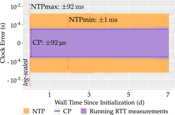
Fig. 1 validates CP as a more accurate inter-node duration measurement method than NTP. CP uses minimum round-trip time (MinRTT) to relate two inter-node TSC values with a microsecond-level error bound. A TSC is nonstop, which resides in a CPU and runs at a constant rate; therefore, it is a qualified source for measuring single-node durations [24]. However, it cannot measure inter-node durations because TSCs on different computers boot at different times and run at different rates. CP presents a reference TSC, pursuing the advantage of using a single TSC for duration measurements. Two MinRTT measurements establish a linear relation between the TSCs of two nodes, and one TSC becomes the reference TSC that provides the standard unit time for inter-node durations. Fig. 1 shows that the MinRTT error bound is , and NTP’s accuracy is bounded by the interval . MinRTT is more accurate than NTP, up to three orders of magnitude.
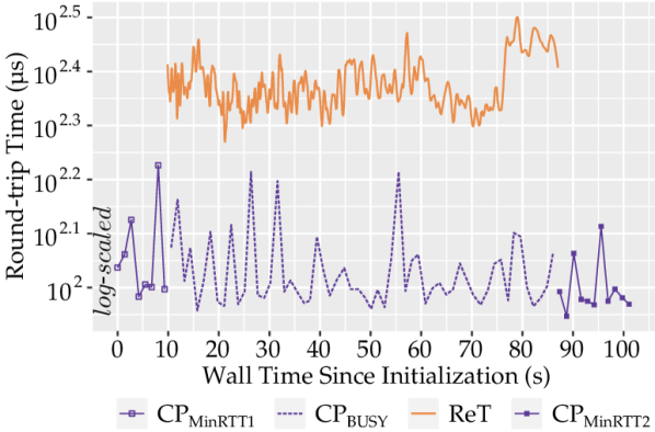
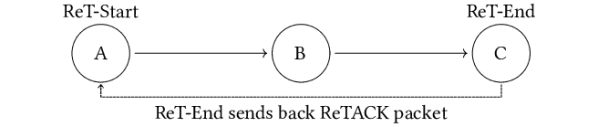
Fig. 2 introduces ReT, another approach to measuring an inter-node duration between start and end events [12]. ReT resends all end events to the starting node and timestamps them as they arrive. It utilizes a single TSC for both events, effectively eliminating the NTP synchronization requirement. However, ReT always incurs an extra duration for resending end events back to the starting node, and the maximum extra duration determines ReT’s error bound. We measure ReT’s error bound by retrieving the RTT of the returned end events. Fig. 2 compares the RTT results of CP and ReT. ReT yields higher RTTs (data series “ReT”) because it competes for the network resource with the ongoing experiment. CP exploits quiescent periods – MinRTT runs before and after the experiment (data series “” and “”). As a reference point, we also ran MinRTT alongside the ongoing experiment (data series “”), which also performed better than ReT.
CP has the following advantages. First, it synchronizes the TSCs in a quiescent period and thus uses the best network condition rather than the current condition, unlike [12] or [25]. Second, it has no dependency on the global clock, unlike NTP. Third, it provides a strict, analytical error bound rather than statistical accuracy [26]. Lastly, it provides off-the-shelf availability on the cloud; it does not require peripheral hardware support such as GPS receivers or Precision Time Protocol (PTP) [27] devices unavailable on commodity cloud nodes.
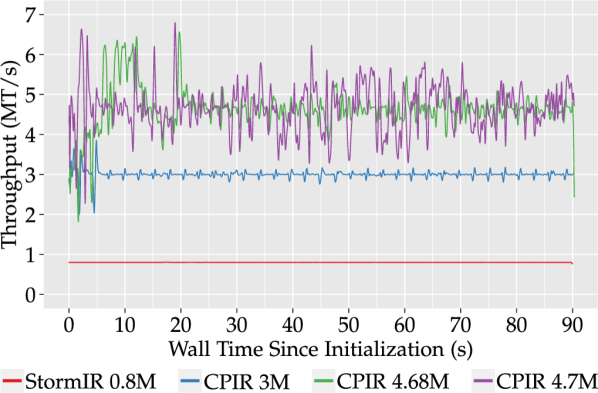
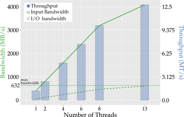
Figures 3 and 4 show our SPE throughput optimization result using our maximum throughput measurement method. An SPE receives unbounded data streams and computes them at the same time. Sustainable throughput [13] is a metric for SPE throughput that continuously lower the emission rate until no tuple backpressure occurs. We propose a maximum throughput measurement method that experimentally evaluates the maximum throughput of an SPE by increasing the emission rate with a C++ throughput-controlled emission loop and a Java object factory (JOF). If the SPE does not drop any tuples at a constant emission rate, we repeat the experiment with an increased emission rate. We do this iteratively until the SPE exhibits a tuple drop, and we pick the last successful throughput as the maximum throughput.
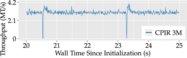
In Fig. 3, we show the result of the maximum throughput measurement method on an unoptimized Storm SPE (StormIR) and the ingestion rate of a Storm SPE with our optimization (CPIR). Using our method, the maximum sustainable throughput of CPIR is . Fig. 4 magnifies the fluctuation at the rate of ; we discovered that it is caused by the Java garbage collector when there is no space for new allocations, especially deserialized Java strings. This paper makes the following contributions.
-
1.
We propose CP inter-node measurement method that is accurate to across two nodes in the cloud.
-
2.
We measured the maximum error bounds of Ethernet-based measurement methods on 30 cloud nodes. Our experiment proves that the CP method is the most accurate on commodity cloud nodes.
-
3.
We measured an SPE can ingest tuples at constant throughput of at the maximum.
-
4.
We propose a CP cloud profiling framework, written in C++ 11 for native platforms, providing platform-independent APIs that log a tuple with or without compression in and , respectively.
The remainder of the paper is structured as follows. In Section 2, we discuss existing measurement methods, including the NTP-based measurement method and the ReT-based measurement method [12]. Section 3, describes the proposed method and its accuracy using the MinRTT of two TSCs on each computer. In Section 4, we discuss our maximum throughput measurement method that correctly evaluates the throughput performance of an SPE using throughput-controlled emission loops and the Java object factory. In Section 6, our proposed validations are explained, including ReT validation and TSC validation. Section 7 describes our experimental setups, implementation details, and conducting details of the streaming benchmark. Then we evaluate the experimental results. Section 8 introduces prior works that precede our inter-node measurement methodology and compares the contributions. We draw our conclusions in Section 9.
2 Background
2.1 NTP-based Measurement and Clock Error
Traditionally, and until now, most time duration measurement in Java applications – in a single node or across nodes – has been done by comparing the System.currentTimeMillis() timestamps. There has been no awareness of Network Time Protocol (NTP) synchronization, which uses a hierarchy of computers synchronized to a reference clock [28].
| Variable | Name and Description |
|---|---|
| root_delay is the total sum of round-trip delay that should compensate network asymmetries inherent to all packet delays from a local computer to the primary server (stratum-1) which has a locally attached reference clock where all downstream servers and clients are ultimately synchronized to. | |
| root_dispersion is the accumulated dispersion over the network from the primary server, where dispersion represents the maximum error inherent in the measurement at each level between two consecutive servers. | |
| system_time_offset is the remaining offset to be slewed off from the local clock. |
| (1) |
An error bound is the minimum or the maximum error of a measured quantity. Inequality (1) states the maximum error bound for the offset of the time-server clock relative to a computer’s local clock, as specified in the NTP v4 standard document [11]. An NTP client polls a sample for each unit time and stores the sample in a list, then selects the best sample that chooses root_dispersion and root_delay for wall-clock synchronization. It adjusts the clock at a maximum of (i.e., adjusting one second requires ) [29] toward the global clock, and system_time_offset denotes the current offset of the local clock.
2.2 Return-trip Method (ReT) Event Occurrence
Off-the-shelf cloud nodes employ NTP to synchronize their clocks to a global reference clock. Assume a tuple processing as illustrated in Fig. 5. A duration starts in Node at time and ends in Node at time . Note that and occurs on nodes and , respectively; using time duration introduces a millisecond or higher error bound.
ReT [12] eliminates the problem of NTP that incurs millisecond-level error bound by reading the global clock within a hierarchy of NTP servers, denoted as a root delay in Inequality 1. ReT avoids the use of TSC values generated on different computers. To measure the latency of , sends back an ReTACK to , which arrives at . Note that and are generated on ; ReT replaces the the time duration with the time duration . ReT eliminated the inaccuracy of NTP at the cost of the inaccuracy imposed by the ReTACK packet transfer time. We discuss the detailed implementation and its validation in Section 6.4.
3 TSC-based Inter-node Measurement
3.1 Reference TSC
The CP method enables measuring inter-node time durations at a higher accuracy than existing approaches. Two characteristics of a TSC make a unique clock for individual nodes: (1) nonstop and (2) constant; a nonstop TSC does not stop regardless of the CPU’s current state such as C-States; a constant TSC counts up at a constant rate regardless of the CPU’s clock frequency changes. A TSC on a typical GCE node provides an accuracy of per cycle for measuring time durations on a single node [30]. PAPI is ubiquitous for single-node performance engineering [24]; however it was not available for the multi nodes because of unrelated TSCs across nodes. Thus, we introduce reference TSC – the single TSC for measuring and comparing time durations across nodes. It requires translating a node-specific TSC value to a reference TSC value; to accomplish this, we introduce TSC Ratio, a linear relationship between two TSC durations on two nodes, measured within the same time duration marked by two MinRTTs.
Fig. 6 depicts two TSCs and two MinRTTs. and mark the start and the end of the time durations and . Using the variables in the example measurement in Fig. 6, we introduce two notations: and . Ratio is a ratio between two nodes, and . Time duration represents a time duration between two TSC values and . Eq. (2) holds for a ratio between two TSCs on nodes and :
| (2) |
Propagation of Error. TSC ticks and are approximations of TSC ticks and ; the round-trip time of each MinRTT measurement bounds their errors: we know that happened between and , but we do not know the temporal order between and ; i.e., there exists an between and . A symmetric RTT between nodes and yields ; however, network asymmetries always results in a TSC tick such as , which bounds to a minimum of and a maximum of ; thus, and are incomparable. Using this information, we can declare in the standard error form [31, Eq. (2.3)].
| (3) |
The measured value comprises of two parts: and . We take an example from in Fig. 6 that starts and ends at and . Because we cannot determine , we use , on the halfway between and , as the best estimate of ; we use , half the duration between and , as the uncertainty that bounds the error of .
To aid in understanding the propagation of errors, we will use a specific color () for TSC values with uncertainty in mathematical expressions in the current section, as shown in equations (3).
3.2 Conversion of TSC values between TSC domains
A TSC value is native to the node where it occurs; TSCs on different nodes have different TSC frequencies and they boot at different time. time. Our CP method incorporates a ratio in the translation to make a TSC value available on another node. We show the translation process using the measurement example in Fig. 6. We translate to using the ratio .
We can eliminate the absolute value signs because and .
| (4) |
Calculating involves and : values with uncertainties and ; i.e., also incurs an uncertainty . We can calculate it using the error propagation rule [31, Eq. (3.48)].
| (5) |
We calculate the uncertainty using Eq. (5).
| (6) |
To evaluate the partial derivatives of Eq. (4), we rearrange the equation in terms of and .
Holding constant, we differentiate it with respect to .
Likewise, holding constant, we differentiate it with respect to .
Now we can calculate the total error Eq. (6). We use the largest error for this calculation.
| (7) |
We remove absolute value signs because we know .
Using the standard error form, we can rewrite the final result:
3.3 Translation of a TSC duration
Measuring a TSC duration requires different strategies by identifying the nodes where the start and end events occurred. We distinguish four scenarios: 1) the duration started and ended on the reference node – the trivial case; 2) the duration started and ended on the same non-reference node; 3) the duration started and ended on two nodes including the reference node; 4) the duration started and ended on two non-reference nodes. While the first case does not incur any error, the last case incurs the largest. We devised the CP method to exploit each case. For Scenario 3, we compare our method and the baseline. We explain each scenario using the examples in Fig. 7.
3.3.1 Trivial case: duration on the reference node
This case considers a duration consisting of the start and end events that occurred on the reference node. It does not require translation and thus incurs no error; it is the same as measuring time durations on a computer with PAPI.
3.3.2 Scenario 1: duration on a non-reference node
The TSC duration’s start and end events occur on the same node; Scenario 1 leverages it to reduce the size of the error substantially. It translates Duration into a duration on the reference node .
where
Each MinRTT round trip measures and . Refer to Fig. 6 and Section 3.1 for more details. We evaluate the error using Eq. (5) and Eq. (7), and the resulting error is as follows:
is smaller than because , where is a duration within , which marks the beginning and end of the experiment, that is substantially long.
3.3.3 Scenario 2: duration on two nodes, including the reference node
3.3.4 Scenario 3: duration on two non-reference nodes
Let node be the reference node, and consider a TSC duration between and in Fig. 7. It involves invoking two scenarios, Scenario 2 and Scenario 1. First, perform Scenario 2 between nodes and ; node is the tentative reference node. Then, perform Scenario 1 to translate the duration from node to node . We begin the evaluation between nodes and : let be the TSC ratio between nodes and ; then use Scenario 2, which results in .
Then use Scenario 1 to translate into .
We determine the error with Eq. (5) and Eq. (7).
| (8) |
We know that , where we set the time duration between the start and end of a MinRTT arbitrarily long; therefore, the following holds.
| (9) |
Next, the following equation explains that the ratio requires reading from TSCs on nodes and at the same TSC instances, , and .
In our cloud configuration, the participating nodes A and B are hypervised machines (HVMs), meaning that their TSCs run at a different but relatively similar speed. While exploiting the difference is the key in the CP inter-node time duration measurement methodology, acknowledging their similarity allows us to evaluate the error size; therefore, the following comparisons hold.
| or | ||||
It follows that the size of error incurred by is greater than 0, close to , but smaller than .
| (10) |
Lastly, we can decide the total size of error incurred by Scenario 3. We evaluated the error size Eq. (8) in two parts: Eq. (9) and Eq. (10). We add up the error beginning with Eq. (10).
We know that the size of error incurred by Eq. (9) is significantly smaller than .
Therefore
3.3.5 Baseline: duration on two non-reference nodes
We take the same example used in Section 3.3.4 but demonstrate a relatively trivial approach, where TSC events are translated individually for further arithmetic operations. The overall process is twofold. First, we translate and as follows:
where,
Second, we measure the duration using the translated TSC values:
| (11) |
Eq. 11 allows us to evaluate the overall error . We determine the error with Eq. (5) and Eq. (7). The evaluated error is as follows.
3.3.6 Error size comparison
We evaluated the error size of the trivial case, three scenarios Scenario 1, Scenario 2, Scenario 3, and the baseline in the preceding sections. The following table shows the overall comparison between them.
| CP method | Size of error | Range of error | |
|---|---|---|---|
| (relative to the max error ) | |||
| Trivial Case | – | – | |
| Scenario 1 | |||
| Scenario 2 | |||
| Scenario 3 | |||
| Baseline | |||
Table II shows that our translation strategy with each scenario successfully prevents translatation errors from bloating unnecessarily. Scenario 1 allows translating cycle-level TSC durations, such as computation time on a non-reference node, into the reference TSC cycles. Unlike the baseline that uses Scenario 2 twice, Scenario 3 combines Scenario 2 and Scenario 1, which minimizes the incurred error.
3.4 Timestamp Counter (TSC)
TSC requirements. The CP inter-node measurement method approximates the time duration of a tuple based on TSC values and TSC frequency retrieved from each cloud node. TSC measurement requires the CPU to feature nonstop_tsc and constant_tsc (a combination of the two is equal to invariant_tsc). CPUs with the nonstop_tsc feature guarantee counting increasing its TSC even when the CPU’s C-state increases over C2. The constant_tsc feature guarantee counting the TSC at a constant rate even when CPU frequency changes. Both features are mandatory and generally available on modern Intel x86 CPUs. However, TSC may not increase in a lock step on a system with two CPU sockets or more.
TSC wrapper function. We devised a new function, clock_gettime_tsc, which calls the kernel-provided clock_gettime and the rdtscp instruction. For every tuple that invokes a buffered ID handler, the TSC value and the local clock (CLOCK_MONOTONIC_RAW)’s timestamp will be logged for measuring the duration. (See Section 5.1 for more details on the buffered ID handler.)
4 CP Data Generator
Profiling an SPE requires a data generator that can produce data streams consistently and at a high emission rate. Existing solutions fail in one or both of these requirements.
4.1 Kafka Shortcomings
Apache Kafka [32] is a framework for distributed data generation, and it provides producers, consumers, and a cluster of brokers. A Kafka cluster accepts tuple streams generated by one or more Kafka producers; then, Kafka consumers subscribed to the cluster receive the tuples. Apache Kafka meets the following requirements. First, it provides a high-level abstraction of the streaming architecture. Second, it decouples data generation (Kafka producers) and data consumption (Kafka consumers). Third, it provides a common pattern to the industry [33, 34]. However, Kafka’s high-level abstraction comes at the cost of performance. Prior work [13, 35, 2, 36] evaluated Apache Kafka as a data generator and reported that Kafka became the throughput bottleneck in those experiments. Chintapalli et al. [2] employed multiple Kafka producers to create the required emission rate because a single Kafka producer failed to emit more than . Perera et al. [36] showed that a single Kafka broker deployed in the Yahoo streaming benchmark increases the event-time latency by when increasing the emission rate higher than . Hesse et al. [37] evaluated the performance of Kafka with their in-house data generators [38] and determined that Kafka’s throughput is capped at when receiving tuples from two data generators. Researchers have abandoned Kafka in favor of their data generator design. Grier [35] abandoned Kafka and increased the emission rate by implementing the data generation facility within the SPE. Karimov et al. [13] abandoned Kafka and designed their data generator.
4.2 Consistently High Throughput is Difficult to Achieve
To produce a data stream at a high and consistent emission rate is a challenging task with cloud nodes. Chintapalli et al. [2] reported that individual Kafka producers began to fall behind at around . Lu et al. [39] point out data generation rate is different from the data ingestion rate. Their streaming system, which employs a messaging system such as Kafka, requires the data generation rate to be faster than the data consumption rate to keep the SPE’s ingestion rate. Hesse et al. [37] implemented a data generator [38] as a Kafka producer to measure the attainable ingestion rate of the Kafka cluster. The data generator emits data at a configurable rate. To evaluate their data generator without Apache Kafka, we employed the ZeroMQ throughput test [40]. Instead of using the Kafka producer APIs, we replaced them with the ZeroMQ PUSH and PULL sockets [41]. We employed two cloud nodes running one data generator and one JeroMQ [42] client each. The test ran for , and their data generator achieved with tuple loss. We found that the data generator stops emitting periodically (up to ) due to GC interruptions. To determine the achievable throughput without tuple loss, we iteratively lowered the emission rate to , where the data generator could sustain the throughput without tuple loss. Apache JMeter [43] is a data generation framework for load testing various web applications. JMeter’s workload model simulates multiple users (i.e., multiple HTTP sockets) and request-and-reply sequences by each user. Its highest throughput is with users [44]. Kallas et al. [45] proposed a framework for validating the correctness of processed tuples. They use JUnit-QuickCheck [46] as a data generator, and they reported a maximum throughput of before exhibiting fluctuation. We measured that their data generator could achieve when emitting tuples to a JeroMQ client. Karimov et al. [13] implemented a distributed data generator with a configurable data generation rate, and their data generation rate is faster than the system-under-test (SUT)’s data ingestion rate. They used the following techniques to even out the data generation and ingestion rates. First, they chose to add a queue between a data generator and a source operator to keep up with the data generation rate. Second, they put each pair of data generators and queues on the same machine to avoid network overhead. It has two advantages and a drawback. First, the SUT does not lose any tuples because the queues keep them until the SUT acquires them. Second, the queues ensure a consistent emission rate by their data generators (DGs). On the other hand, their design requires inspection of both the throughput and the event-time latency to determine the SUT’s sustainable throughput. If the SUT does not exhibit prolonged backpressure (i.e., the event-time latency does not increase continuously), the currently configured generation rate becomes the sustainable throughput. They need a way to measure lags-per-second. An ongoing work [47] attempts to provide quantification using lags-per-second. Fig. 9 in Section 4.3 describes our new algorithm to evaluate the maximum throughput of the SUT correctly.
4.3 Throughput-controlled Emission Loop
To address the shortcomings of the existing DG design, we propose a measurement methodology (as in Fig. 9) to correctly evaluate the maximum throughput of the SUT across multiple cloud nodes.
evaluate_max_throughput (Fig. 9a). For all experimental runs, we set a duration of for the current run. SPE runs infinitely in production nodes; however, our measurement methodology incorporates duration for bounding the experiment’s start and end (lines 3 and 4). We increase iteratively for each run until a tuple drop occurs (i.e., the number of tuples generated by the DG sender must equal the number of tuples ingested by the SUT unless a tuple drop occurred). A tuple drop indicates that the last successful throughput is the maximum throughput of the SUT.
emission_loop (Fig. 9b). It guarantees to send each tuple within a unit time by querying the current time now() while it is within the time window (line 11). It ensures the emission loop will send all tuples before the designated time end_loop.
Overhead of a ZeroMQ send call. We ensured that a budget is equal to or bigger than the overhead of ZeroMQ’s send operation ZMQ_Overhead (line 6). We measured that the single-call overhead of ZeroMQ’s send operation is , i.e., one emission thread will not run faster than . It is using a Yahoo streaming benchmark tuple, and a total of nine ZeroMQ threads can emit at () at maximum.
4.4 Tuple Processing with the Java Object Factory
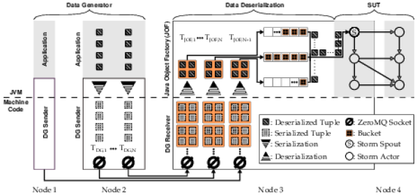
In Fig. 8, DG Sender runs on Nodes 2 and 3 attached to a user application. Assume that on Node 2 in Fig. 8, a user application running on JVM creates an application-specific tuple as a Java object (E.g., Yahoo streaming benchmark creates advertisement information events exposed to a user). We designed DG Sender as Java Native Interface (JNI) machine code built with the user application. DG Sender requires the application to pass the tuple data as a byte array using Kryo [48] for Java object serialization. (Apache Spark [49] and Apache Storm use Kryo.) The application hands over the resulting byte array to thread via the JNI interface provided by DG Sender. DG Sender prepares all tuples serialized ahead of the experiment to avoid Java object serialization overhead from the critical path in the emission loop. In each emission thread, the ZeroMQ socket sends the serialized tuple to the corresponding ZeroMQ socket in a JOF thread on Node 3. JOF is our Java object deserialization library built against the SUT as part of CP. Each JOF thread runs a deserialization loop that pulls out buckets of serialized tuples and pushes each bucket to an SPSC queue after de-serializing all tuples in the bucket. Here, we use Kryo for deserialization, and we take all overhead of deserialization which affects the resulting throughput. We deploy one JCTools [50] SPSC queue in each JOF thread. A Storm Spout in the SUT iteratively drains the queues in the nextTuple() method, fetching one bucket from a queue and ingesting a tuple at a time.
Using JOF, we measured that the SUT can consistently ingest tuples at without exhibiting a tuple drop. It is five times faster than running the same SUT without JOF (). We ran the experiment on seven GCE nodes – three for ZooKeeper, one for Redis , one for Storm Nimbus, one for DG Sender, and one for SUT. We implemented a Storm sink application as the SUT. It receives tuples in the Spout and drains them in the subsequent actor.
5 CP Profiling Framework
CP profiling framework is a native C++ 11 library that implements TSC inter-node measurement method with cloud profiling components.
The latency of event processing times of a streaming engine provides insights into its operational efficiency over time. Because data arrives at high density and velocity and loses value over time, event processing latency is crucial for the perfromance engineering of an SPE.
We tag each event with a tuple ID to trace them and their processing times as they flow through a stream graph topology. We explored relevant software engineering exercises. Retroactive extension [51] describes a software engineering requirement that allows extending a program without recompiling the source code. Manifold [52] is an ongoing attempt that implements such software engineering requirements for Java; however, we discovered that its Extension feature only supports adding a static field to an existing class, whereas we need to inject a unique tuple ID in each tuple object. Thus, we added two APIs in CP for application developers: getBytes() and loadBytes(). A tuple receives a tuple ID using getBytes(), and the function serializes the tuple into a byte array. CP then preloads the byte array for data generation with loadBytes().
To avoid perturbing the Java code running on the streaming engine, we designed CP native library to conduct all high-resolution time measurements in machine code. As depicted in Fig. 10, our approach is minimally invasive. The SUT only needs to open channels, which to the JVM, are represented as values of primitive type long. (We defer the discussion of the channel’s handler argument to Section 5.1.) After an invocation of the function openChannel() (line 5), logTS() (line 10) allows logging a timestamp, tuple ID pair. The CP framework stores such log information in each channel’s underlying log file. Log files are collected post-mortem for retrieval of profiling information.
Assigning each event a unique tuple ID and inserting instrumentation similar to Fig. 10 make it possible to trace a tuple through the stream-graph topology at nanosecond resolution. Particular points of interest and instrumentation in the application code are the start and end of an actor’s work function and calls to receive and post tuples.
5.1 Handlers and Trace- and Sample-based Profiling
The C++ 11 native APIs are exported to JNI using the SWIG-Java library [53]. Thus, we can instrument both C++ 11 and Java programs with our CP library. We demonstrate the use of the library in Fig. 10. The CP native library loads once per JVM instance (line 3). Opening a profiling channel requires a channel name, log format, and handler type (lines 5–8). For the current channel ch0, the library logs a TSC value, tuple ID pair, effectively distinguishing each tuple (line 10). The timestamp comes from the rdtscp() instruction. Closing a channel causes buffered logging data (if any) to be flushed to a disk. As depicted in Fig. 11, a closure [54] represents a profiling channel, which contains a pointer to the channel’s handler function (line 2) and the entire referencing environment (data) of the handler. (Complex handlers, e.g., an FIR filter, can extend the closure type by adding the required book-keeping information.) A handler function receives its closure as a type-erased argument [55] to avoid the overhead of a dynamic (dispatching) method call. Internally, the channel ID of type long from Fig. 10 is a pointer to the channel’s closure. Procedure logTS() calls the closure’s handler with the closure as its argument. Handler functions are type-specific and thus able to regain the closure type through a C++ static cast [56]. We optimized the handler dispatching mechanism for logging events in streaming workloads at nanosecond-level accuracy. The parm_handler_f function pointer (line 4) lets handlers incorporate a function that parameterizes the handler. We provide several types of handlers to conduct trace- and event-based sampling. A handler associates with a channel opened (see Fig. 10, line 8).
Identity handler (ID handler). This handler writes the TSC value, tuple ID pair verbatim to the channel’s underlying log file.
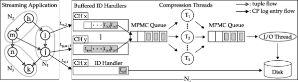
Buffered identity handler (buffered ID handler). It buffers the TSC value, tuple ID data, performs in-memory compression, and writes them to the channel’s log file. As shown in Fig. 12, the handler initializes with multiple blocks, and each block can store tuples (a compile-time constant). Instead of writing each logged tuple directly into the channel’s log file, it buffers tuples into the blocks. We employ the non-blocking Michael-Scott queue [57] from the Boost C++ libraries [58] for moving blocks. A block is enqueued into the boost MPMC queue when it becomes full. When a block is full, it is enqueued into the boost MPMC queue. We employ multiple compression threads to dequeue and compress blocks and enqueue them into the I/O queue (another Boost MPMC queue). The I/O thread dequeues the compressed blocks and writes them into the corresponding log file with its channel. For termination, CP registers a callback function that activates with a SIGTERM signal. Termination begins with closing all associated channels; it stops ingesting new data and flushes the processed data left in the system, ensuring no log data is lost.
Periodic counter handler (PC handler). It counts the number of tuples read within a period of specified duration. At the beginning of each period, the periodic counter resets and starts from zero. When the channel closes, all periodic counts accumulates into the total count. The PC handler consumes fewer resources than the ID handlers and determines the changes in throughput during the benchmark run. We employ a sampling thread that maintains the start of all periods in a lock step. We propose two versions of the PC handler. First, a single-threaded periodic counter handler (SPC handler) provides optimized performance when deployed on a dedicated core. It uses a relaxed memory operation for counting tuples and ensuring the value is globally visible when the sampling thread accesses the variable. Second, a multi-threaded periodic counter handler (MPC handler) uses acquire-and-release memory operations, which gains performance across threads. We found that the MPC handler runs at while the SPC handler runs at , increasing the performance three. The complete result is in Table V.
Downsample handler. This handler logs every tuple/timestamp to the log file and discards tuples otherwise to reduce profiling overhead. A channel acquires the argument via the channel’s parameter handler.
XoY handler. It receives two arguments: and . It logs a timestamp, tuple ID pair to the underlying file iff.
For example, assume and . The handler logs tuples , and subsequent. This handler allows conducting sample-based logging tailored to batches of tuples. The advantage of this tailored logging is that the same batch of tuples will show on all channels that use the same argument values and ; thereby, it becomes possible to compute durations for a given tuple. (The calculation is impossible if a tuple were kept on one channel but discarded on the next channel that this tuple passed through.)
FirstLast handler (FirstLast handler). It writes tuple ID, TSC pairs of the first and last tuples processed by the streaming application. The handler avoids the overhead of logging all tuples and provides the first and last timestamps for calculating the overall tuple processing time.
Return-trip handler (ReT handler). The handler reproduces the ReT measurement of a streaming application. We described the ReT method in Section 2.2.
Null handler. It discards tuples from being logged. It provides a convenient way to temporarily disable unused channels via the configuration server (See below for a detailed explanation) without rebuilding and deploying the target application on cloud nodes.
Online Handler Configuration. CP provides online handler configuration via the configuration server. It
opens a handler channel, it retrieves the handler type associated with the channel name.
All artifacts, including the native CP library and the measurement data, are available [59].
5.2 MinRTT Measurement
CP provides server and client applications for the MinRTT measurement: TSC server and TSC client. We employ a TSC server that conducts the measurement across TSC clients. We employ one TSC client on each node inside the experiment; its task is to retrieve a TSC value from a corresponding TSC client while measuring the RTT. The goal of this measurement is to achieve the following information.
MinRTT. The MinRTT of two nodes Node and Node determines a temporal order of TSC values measured on the two nodes. A MinRTT packet that leaves and comes back to Node via Node generates three TSC values – start and end TSC values on Node and a TSC value on Node that happened between the start and the end. MinRTT conducts several RTTs and selects one with the minimum round-trip time.
TSC frequency. We use TSC frequency when representing our experimental data in seconds rather than the TSC cycles. We conduct all experiments in native TSC cycles and use the CP method to translate them to the reference TSC cycles. Only then we use the reference TSC frequency to increase readability. We do not use the kernel-calculated TSC frequency but calculate it ourselves using two MinRTTs ( and in Fig. 6) to tighten the error bounds of oscillators aging and prone to thermal changes [7].
Once the TSC server has all TSC clients registered, it requests MinRTT measurements from every TSC client pair. The MinRTT measurement considers directions and because network conditions and routes may vary. Upon receiving a MinRTT request, each TSC client pair runs several iterations of RTT measurement and send back the MinRTT value to the TSC server. By the end of all MinRTT measurements, we obtain MinRTT for every node pair.
6 Validation
6.1 Validation Setup
We ran all validations on cloud nodes in GCE. We describe setups for each validation.
Non-virtualized TSC. To validate whether TSC is virtualized or not, we employed one node . For comparison, we used Intel Skylake i-5 6600 machine.
ReT method. We employed two nodes for a ReT method validation. ReT method requires two nodes: one for ReT-Start and the other for ReT-End. Each has eight vCPUs and RAM. We wrote the validation in C++.
CP method. We employed 30 nodes to run the CP method with the Yahoo streaming benchmark [2]. Yahoo streaming benchmark is an off-the-shelf benchmark that provides a baseline environment to execute the company’s in-house streaming application on a single server, and we extended it to suit our multi-node configuration. Our cloud resource includes 488 vCPUs and of RAM; the Storm framework uses over two-thirds of the vCPU resources. Each of the 10 Storm worker nodes has 32 vCPUs and RAM, and one node exlusively runs a Storm Nimbus, which is responsible for scheduling. Another 10 nodes run cloud infrastructure applications, including ZooKeeper, Kafka messaging queue, and Redis in-memory database. The remaining 10 nodes run data generators that feed data into Kafka brokers. The benchmark is available online on GitHub [60]. We selected Apache Storm 2.0.0 to run the benchmark application. We used ZooKeeper 3.5.5, Kafka 2.3.0, Redis 4.0.11, and Storm. All JVM processes of the benchmark ran on Oracle Java 8, and all nodes ran Cent OS 7 Linux. We used GCC 8.3.0 to build CP-instrumented cloud applications with libraries SWIG 2.0.10, ZeroMQ 4.1.4 [61], and Boost 1.61.0.
CP compression. To validate the bandwidth and scalability of the ZSTD compression in CP’s buffered ID handler, we employed a node with 56 vCPUs, of RAM, and a local scratch SSD.
CP overhead. To validate the performance overhead of CP, we employed 10 nodes to run the Yahoo streaming benchmark.
6.2 TSC Validation in the Cloud
Invoking rdtsc and rdtscp should read the underlying CPU’s TSC register, and we need to validate that GCE’s KVM does not virtualize TSC instruction results. First, we ran rdtsc and rdtscp instructions iteratively times. Second, to prevent out-of-order execution by the CPU, we reran the same test times.
Invoking rdtsc on a cloud node took for both iteration setups. Running it on an Intel i5-6600 took for iterations and for iterations. We ran the same test for rdtscp, which took on the cloud node. On an Intel i5-6600, one invocation took for iterations and for iterations. The comparison between a cloud node and the i5-6600 bare metal system shows that GCE’s KVM does not virtualize either rdtsc or rdtscp, and the instructions are usable for our CP method. Invoking rdtscp is slower than rdtsc because it provides additional information, such as CPU processor and socket numbers [62].
6.3 CP Compression Bandwidth and Scalability
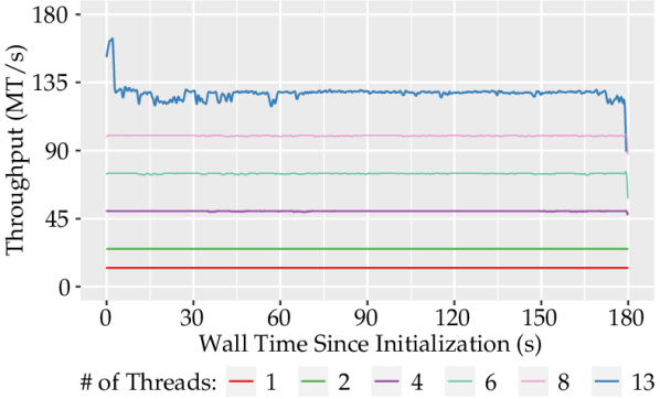
Figures 13 and 14 show the scalability of the buffered ID handler. We use the Squash compression benchmark [63] to run and compare different compression algorithms. We chose the ZSTD compression algorithm because it shows a high compression rate and fast compression speed for compressing CP’s ID handler logs.
We validated CP’s logging compression and scalability performance on a node with a local scratch SSD disk. Google reported the sustained throughput limit of and for read and write operations, respectively. We also benchmarked the local scratch SSD disk using the fio tool [64] and measured the maximum disk bandwidth of for sequential write operations. We used the same fio parameters that Google provided [65], but we did not set direct and end_fsync to make the behavior of the I/O operations identical to CP’s I/O.
We set each thread to write tuples at constantly and scale the number of threads until we get the maximum disk bandwidth. As shown in Fig. 13, we can achieve scalability up to eight threads, but the test with 13 threads cannot achieve the required throughput of .
In Fig. 14, Buffered ID handler achieves with 13 threads, which is close to the maximum disk bandwidth of that we measured with fio tool. Note that they are compression performances; the uncompressed data throughput is . The ZSTD codec performed the compression ratio of .
| C++ | Java | ||||
|---|---|---|---|---|---|
| Latency | Throughput | Latency | Throughput | ||
| 100M Iterations | (ns) | () | (ns) | () | |
| CP Handlers | ID | ||||
| Buf. ID bin | |||||
| Buf. ID zstd | |||||
| Buf. ID lzo1x | |||||
| Downsample | |||||
| XoY | |||||
| SPC | |||||
| MPC | |||||
| Null | |||||
As shown in Table III, we compared the single-thread performance of various CP handlers on a cloud node. PC handlers– SPC handler and MPC handler outperform other handler types because they only log the number of logTS() calls for each unit time. A buffered ID handler does the same logging like an ID handler does, but it outperforms and logs at up to several million tuples per second with the help of the underlying compression threads. The JNI overhead causes all CP handlers to exhibit lower throughput on a Java program than on a C++ program.
6.4 ReT Method Validation in the Cloud
We compared our CP measurement method with NTP and ReT to validate its accuracy. To reproduce the ReT measurement, we added ReT-Start and ReT-End handlers to the CP library. We ran ReT-Start and ReT-End programs on two cloud nodes.
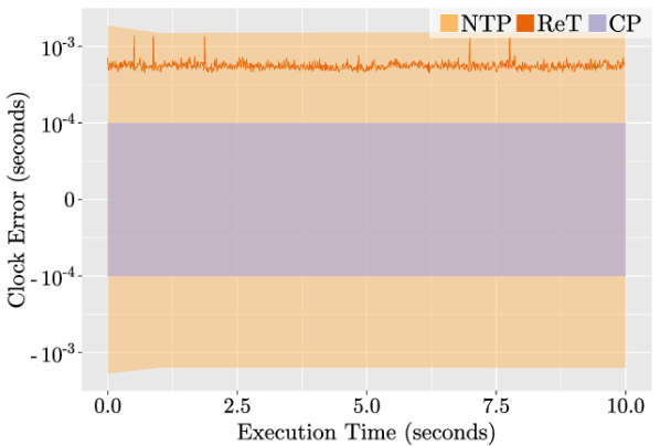
Fig. 15 depicts that CP achieved the lowest and constant error bound . ReT method resulted in the average lower bound of with minimum and maximum lower bounds of , respectively. NTP’s clock error decreases over time during the validation, which marks a minimum lower bound of and a maximum upper bound of . A detailed account of how we determine the clock error of the CP method on cloud nodes is in Section 6.5.
6.5 Validation with the Yahoo Streaming Benchmark
To validate the CP method in a production-level environment, we ran the Yahoo streaming benchmark with CP instrumented in the source code and compared its error bound to the error bounds of NTP and ReT methods. We ran the validation on GCE nodes with the following design considerations.
Minimum round-trip time (MinRTT). TSC clients on all possible unique pair of nodes measure MinRTT. Each pair exchanges measurement packets 100 times to select MinRTT for the pair. The TSC server receives all MinRTT results.
NTP clock error. To calculate the error bound of the clock error at the current second, system_time_offset, root_delay, and root_dispersion values are retrieved by invoking the chronyc command every second for the entire run of each cloud node.
ReT method error bounds. We implemented and incorporated the ReT handler in CP to run the ReT method. The handler consists of ReT-Start and ReT-End handlers, and they measure the RTT of each ReTACK packet.
CP instrumentation. We instrumented the Yahoo streaming benchmark with CP handlers. We added a ReT-Start handler to the DGSpout actor and a ReT-End handler to the benchmark application’s CampaignProcessor actor. DGSpout receives all incoming tuples coming to the streaming system, and ReT-Start handler assigns each of them with a start time; therefore, it is where all ReTACK packets return to and receive an end timestamp. When a tuple arrives in CampaignProcessor class, the ReT-End handler sends back a ReTACK packet to the ReT-Start handler in the DGSpout. The ReT-End handler measures the RTT, and both handlers log the start and end timestamps.
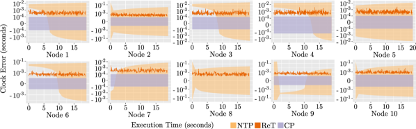
In this experiment, the benchmark ran for after Storm scheduled the streaming application, mapping it across 10 worker nodes. The ReT method intends to run on a single source actor; therefore, we configured Storm to allocate one DGSpout. In Fig. 16, DGSpout was allocated to Node 8 to receive tuples from the Kafka cluster.
Fig. 16 shows the clock errors of the compared methods. We prepared diagrams for individual nodes because the TSC count and TSC increment in each worker node have unique values; likewise, for two computers with the same CPU, their TSC value and TSC increment will not be the same; booting time will make the TSC count different, and CPUs on the two computers will run at a different speed; also, NTP clock error of each compared nodes is always different because of the network.
Diagrams in Fig. 16 show that the NTP clock error is unstable and increases over time on every worker node during the experiment. The diagram is also similar to Fig. 15. The CP method retrieves required system information, including each node’s TSC count and TSC increment during the quiescent time – before, after, and in-between network communication bursts; however, ReT and NTP method must be running in real-time, during the experiment. The error bound of the benchmark shows a crucial advantage inherent to the CP method.
The NTP clock-error bar in nodes does not include during a specific period of execution time because the system clock is away from the desired global clock in the NTP hierarchy. The NTP protocol monitors the system time offset from the global clock and applies this information to re-calibrate its system clock. Global clock information, on the other hand, is transferred in NTP packets sent from peer clients on the network in the subscribed NTP hierarchy. Because an NTP packet includes information about the network uses, a less congested network will contribute less to clock errors. However, a streaming application that sends more than data packets per second between nodes cannot expect a quiescent network. Because the system wall clock is consistently re-calibrated by the NTP client, our evaluation is to avoid using the system clock in measuring durations between cloud nodes and on a stand-alone system where the required measurement accuracy is sub-millisecond.
ReT method, by its design, accumulates half the RTT at minimum when measuring a time duration across multiple nodes. The ReT error bounds depicted in Figures 16 and 15 address the glaring overhead.
Conversely, the CP method exhibits the smallest and constant error bound over execution time. As mentioned, we can retrieve the required TSC values in a quiescent period.
Node 8 of Fig. 16 does not include CP error bound because a DGSpout actor resides created in the node. CP method is not measurable for a tuple that has ended up in the actor where it originated. Our implementation of ReT-method does not consider this case. The original work does not mention specific cases but only cases where ReT-Start and ReT-End nodes differ.
The result shows that CP’s smallest error bound was between , and its largest error bound was between . ReT method showed an average of , , and as the minimum and the maximum, respectively. NTP method’s clock error showed and as its minimum lower bound and maximum upper bound, respectively. (We do not use the results from those nodes where the wall clock offsets have gone off from .) The biggest absolute error-bound size measured was from the previously selected minimum lower bound and maximum upper bound. This pair was measured on Node 2 at the first second into the benchmark execution. MinRTT may vary on different instantiations of the same node. The maximum MinRTT we measured is .
6.6 CP Instrumentation Overhead
| Configurations | Min | Max | Med | Avg | CoV |
| CP handlers | |||||
| Null handlers | |||||
| No handlers | |||||
| (Unit: , except for CoV) | |||||
In this part, we determine the performance overhead of the CP-instrumented code and show that the yielded overhead is marginal compared to the non-instrumented version. We instrumented the PC handler in all actors of the Yahoo streaming benchmark and ran it on GCE nodes. Second, we ran the same configuration but with all handlers nullified. Lastly, we ran a version where we removed all instrumentation in the source code. To measure the performance of the three configurations, we used FirstLast handlers, which log the first and the last tuples to determine the overall processing time, and we used PC handlers in sink actors to count the number of processed tuples. As a result, in Table IV, the CP-instrumented Yahoo streaming benchmark runs at on average, while the non-instrumented version runs at . We measured that the CP-instrumented code yields overhead on average and overhead in the median.
7 CP Deployment: Measuring of Latency and Throughput
7.1 Analysis of Tuple Processing Latency
In this section, we demonstrate how we used CP for the tuple latency analysis of the Yahoo streaming benchmark and explain the significance of CP, not only for the benchmark but for the inter-node time duration measurements across cloud nodes. We used the same cloud configuration for the Yahoo streaming benchmark in Section 6.5. In this experiment, we maximized the incoming rate of streaming data by enabling all five source actor instances, which is different from the setting we used for the validation, where we deployed a single instance of source actor to enable the ReT method for the validation.
The benchmarking application has buffered ID handlers instrumented at the beginning and end of the tuple computation in all actor instances. It allows measuring the tuple computation time and the time durations of all tuple transfers between any two actors. For a tuple that has traveled the entire benchmark topology from DGSpout to CampaignProcessor, its end-to-end latency can be measured by relating two TSC values, one from DGSpout and one from CampaignProcessor; likewise, the CP method can measure actor-to-actor latency by making a relation using TSC values from two consecutive actors.
Tuple transfer latency is a time duration of a tuple that has transferred from one actor to another. Tuple processing latency – the total processing time of one tuple throughout the topology – is a tool to assess the performance of a big data streaming topology. We measure tuple transfer latency between two actors, and the two actors may or may not be connected directly. Tuple processing latency is a partial case of tuple transfer latency where the two measured actors are starting and end actors.
Poison pills enable measuring a time duration on unbounded data streams across multiple nodes. It takes the following steps: a streaming application launches and starts emitting tuples. FirstLast handlers instrumented in the source actor instances recognize the first arriving tuple and timestamp it as the start of the measurement duration. Second, the streaming application emits poison pills to notice the end of a period, and the poison pills start filling up the application topology. Lastly, FirstLast handlers in the sink actor instances recognize the first arriving poison pill and mark the ending time. Having a total order of start and end times, we can calculate the length of the period using the earliest starting time and the latest ending time.
By instrumenting FirstLast handlers and buffered ID handlers in this benchmark, we measured that the benchmarking topology in this experiment ran for , processing tuples during the run.
The latency between any two actors can be measured using buffered ID handlers instrumented in every actor of the benchmarking topology. In each actor, two buffered ID handlers log a tuple ID and a TSC value at the start and the end of the tuple computation for every incoming tuple. We can calculate the tuple transfer latency using the TSC values of two actors in which a tuple started and ended. The selected actors may or may not be connected; the end-to-end latency of a tuple in the target topology is the case when we choose TSC values from a source actor and a sink actor.
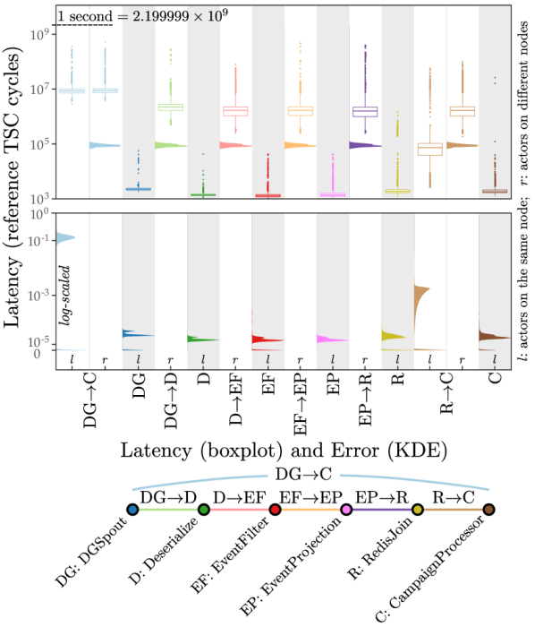
Fig. 17 shows the experimental results of the tuple transfer latency between two actors. The -axis denotes the reference TSC cycles to depict latency and error, and the -axis denotes either an actor pair or an actor by itself; each actor pair shows inter-node latency (tuple transferring time between two actors); each actor on the -axis shows tuple computation time. For example, DGC on the leftmost side of the -axis is an actor pair, and its boxplot shows tuple transfer time between the two actors DG and C. Next to DGC is DG – its boxplot shows tuple computation time on the actor DG. different latency groups – end-to-end (DGC), actor-to-actor (DGD, DEF, EFEP, EPR, and RC). Depending on the communication distance between the measured actors, the latency result splits into two sub-groups – remote and local; the inter-node tuple transfer latency as the remote group, and the node-local tuple transfer latency as the local group.
We present the result using a boxplot. The width of a box represents the number of latency-data points used to draw it. A black dot inside the box shows the mean value of the latency group. A band within the box represents the median or the \ordinalnum2 quartile (Q2) (i.e., the \ordinalnum50 percentile). The box’s floor and ceiling denote the \ordinalnum1 quartile (Q1) and the \ordinalnum3 quartile (Q3). The height of the box represents the interquartile (IQR). The vertical lines connected to the above and the beneath are whiskers, which represent the ranges and , respectively. Each whisker ends with a bar that denotes the maximum and minimum valuew and the minimum value omitting outliers. A group of vertically aligned dots above and beneath a whisker is outliers. We present the error distribution of each box as a kdernel density estimate (KDE) diagram. The remote groups yield a maximum error of and a minimum error of . The local groups yields a maximum error of and a minimum error of . Intra-node durations incur errors because we translate them into the reference TSC cycles. The error results do not include time durations on the reference node because they do not incur errors.
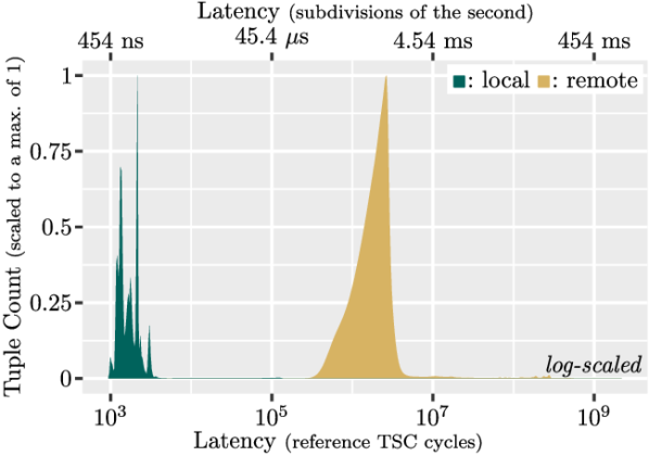
End-to-end latency is on the leftmost of Fig. 17. It measures the tuple transfer latency between DGSpout and CampaignProcessor. Because it accumulates the tuple computation time of the intermediate actors between the source actor and the end actor, it is also called end-to-end processing latency or tuple processing latency. The result splits into remote and local. Remote latency is the time duration between two actors that reside on different nodes, and local latency, on the other hand, is the case where the two actors reside on the same node. Local latency, however, is not limited to the case where tuples stay on the same node during the whole process; instead, it includes a multi-node-traveling case where tuples begin and end on the same node but move to other nodes during the processing. This case is effectively depicted in Fig. 18 – most of the tuple latency equal or greater than belongs to the remote latency. However, some cases in the local tuple latency are longer than because they belong to the multi-node-traveling case. The diagram intuitively differentiates end-to-end tuple processing latency from the local latency to the remote latency – the remote tuple transfer latency is mostly around , slower than the local tuple transfer latency. The interquartile of the remote end-to-end latency in Fig. 17 also covers the latency, which supports the result from Fig. 18. The result shows a glaring result that we cannot measure inter-node time durations within the accuracy of with the NTP-based measurement methodology, which has an error bound of at the minimum.
Actor-to-actor latency exhibits the tuple transfer latency of two consecutive actors. The result exposes Storm’s default orchestration strategy prioritizes vertical scaling over horizontal scaling; i.e., the actor-to-actor latency group does not have a remote group except for the RedisJoin to CampaignProcessor group. It means that every tuple that has started from a source actor on a specific node stays on the node until it reaches RedisJoin. For those local groups, tuple transfer latency stays below . We can also discover that the number of tuples decreases as the tuples go through EventFilter.
8 Related Work
Kieker [66, 67] is a profiling framework for monitoring concurrent or distributed software systems. It is suited for the situation when the users want to monitor and figure out the performance leaks. Except for general monitoring for Java-based systems, Kieker supports various features, including failure diagnosis and performance anomaly detection [68].
While both CP and Kieker performance measurement tools, they have different features. Kieker runs above JVM, while the CP can run on native C++ through JNI. Thus, CP can get performance measurement with an overhead of nanoseconds through native calls, but Kieker takes microseconds to get it with JVM overhead. For example, it takes to call a single method on an enterprise server machine, including instrumentation, collecting performance data, and writing them to a file system [67]. On the other hand, a single call for CP buffered id handler takes less than . CP can get the high-resolution time measurement using system calls, but Kieker cannot since Java does not provide measurement API with nanosecond granularity [69].
Several researchers have discussed the performance of Kieker [68, 70, 66]. In [66], the authors of Kieker deployed Kieker in a real-world multi-user Java web application, and they report that Kieker incurs server-side response time overhead.
Kieker can be used to monitor and analyze general big data applications. On the other hand, CP is an event-based performance profiler with various types of handlers. It is specialized for streaming applications, synchronizing over different nodes using TSCs to provide accurate inter-node time latency between multiple nodes; moreover, CP can measure the target system’s maximum sustainable throughput.
| Latency | Throughput | ||
|---|---|---|---|
| 100M Iterations | (ns) | () | |
| Kieker | EmptyRecord | ||
| TimestampRecord | |||
As shown in Table V, we check the single thread performance of Kieker monitoring records on GCE. While the handlers of CP can process at least several million tuples per second as shown in Table III, the maximum throughput that Kieker can get is around .
Both the authors of [2] and [13] use NTP to synchronize the time among multiple nodes; however, Dongen et al. [22] note that NTP is only accurate to a minimum error of for synchronization [19]. They propose an approach similar to [12], where they use a single Kafka broker to improve synchronization accuracy up to the millisecond level; however, in their sustainable throughput measurement, they used a multi broker Kafka cluster which relies on NTP because a single Kafka broker cannot emit high throughput to measure sustainable throughput of SPEs. To increase the accuracy of latency measurements, we propose CP method which has an error bound equal to the MinRTT between two nodes.
Ridoux and Veitch present the software-based TSCclock [26, 71, 72], which performs between the sub-microsecond accurate PTP and the one millisecond accurate NTP for measuring time durations on a single computer; however, the TSCclock method has not been designed for the measurement of inter-node durations for performance profiling and has the following disadvantages compared to the proposed approach. First, their approach introduces clocks, establishing a notion of global time. The conversion of TSC cycles to seconds requires the TSC frequency, or in other words, , an estimate of the average CPU oscillator period . A typical quartz yields an error of 20 microseconds per second due to thermal changes [7], and incorporating an oscillator period increases the error above the required accuracy. Second, to measure the time duration between a start event and an end event, the 10-microsecond accurate difference clock requires the two events to be from the same TSC so that the initial offset K in both timestamps cancel each other, i.e., the difference clock is incapable of measuring the inter-node time duration between two TSCs because the two timestamps have different Ks. Third, the work does not provide a strict error bound on the obtained accuracy of the and clocks. They provide statistical accuracy with a median and an IQR of their error. Fig. 3 of [26] shows an error value higher than at specific instants, larger than the median of , and an IQR of . It means that the error of inter-node time duration measurements between two nodes can be as high as ; likewise, their absolute clock has , the current estimate of the uncorrected clock. Its median error is , which is not bounded [71, 72]. When measuring the inter-node duration between two nodes, the errors of the two uncorrected clocks add up. Lastly, the proposed approach requires kernel modifications to timestamp incoming and outgoing UDP packets. Modifying the host kernel from the guest OS is infeasible in hypervised environments such as public clouds.
The timestamp-counter-based precise Relative Clock Synchronization Protocol (TSC-RCSP) [73] achieves a 10-microsecond accuracy for measuring the relative offset between clocks. It uses TSC values and the TSC frequency to measure the time offset between two clocks. They calculate the frequency every to mitigate the problem with the oscillator frequency error. TSC-RCSP has the following shortcomings. First, the protocol requires a modified network interface card (NIC) to acquire timestamps. They developed a kernel module to calculate the TSC frequency periodically; however, such a modification is infeasible for the guest OS in a hypervised environment. Second, the error of TSC-RCSP is not bounded. TSC-RCSP guarantees a synchronization accuracy of with confidence. Third, TSC-RCSP does not target general-purpose communication networks, e.g., LAN or the Internet. Instead, the authors designed the protocol for distributed real-time control systems, where real-time support is assumed, and fixed-size packets travel via a control network.
Chen and Yang propose a clock synchronization scheme using a Time Synchronization Function (TSF) counter available in Wi-Fi network cards [74]. The authors emulate a hardware PTP clock using the TSF counter and show that they achieve -level accuracy between Wi-Fi devices.
The authors of [25] describe the algorithm that compares the accuracy of the One-Way Delay (OWD) estimation mechanisms. OWD is a formal estimation of half the RTT, i.e., . This informal estimation average (av) can not be the true OWD because network time always differs on the way to a target node and the way back to the originated node. In this work, the authors propose a way to formally compare their previous contribution minimum pairs (mp) to the informal estimation algorithm.
Time-of-Flight Aware Time Synchronization Protocol (TATS) [75] is a multi-hop time synchronization protocol for energy-consumption-aware wireless devices which achieves sub-microsecond synchronization error. It tackles the propagation delay problem between antennas by applying compensation to each link with an estimated delay shipped on a message.
Researchers have observed that SPEs start to exhibit backpressure when the tuple arrival rate exceeds the processing capacity of the SPE. A widely used data generator, Apache Kafka, suffers from low throughput, capped at [37]. The backpressure issue requires well-defined criteria for how much throughput the streaming frameworks can process without backpressure.
Karimov et al. [13] newly defined and measured, sustainable throughput that previous work, such as the Yahoo streaming benchmark [2], omitted. The authors define sustainable throughput as the highest load of event traffic that a system can handle without exhibiting prolonged backpressure. Dongen et al. [22] further extend the notion of sustainable throughput by defining maximum threshold values for latency and CPU utilization.
Both works [2] and [22] used Apache Kafka as a data generator. A single data generator of [2] falls behind at around 17,000 events per second. [13] mentions that Apache Kafka and Redis are the bottlenecks of the Yahoo! Streaming Benchmark [35]. They choose to generate data on-the-fly and eliminate fluctuations due to network issues and GC interruptions.
A large body of work [2, 22, 39, 76, 77, 78, 79, 80, 81, 82, 83] used Apache Kafka as a data generation facility for benchmarking streaming frameworks, as it is a widely used message broker. It was pointed out in [39] that Kafka could be a bottleneck due to their data generation speed and messaging processing capability. Researchers proposed workarounds to mitigate those limitations of Apache Kafka. To ensure that Apache Kafka does not degrade the performance, Lu et al. [39] preloaded and replayed a set of records during the experiment to avoid the data creation overhead. Nasiri et al. [79] ran Kafka in a separate machine. Karimov et al. [13] abandoned Kafka and created new data generators to overcome the bottleneck and generate the data on the fly. Shukla et al. [84] implemented a scalable data-parallel event generator that acts as a source task for IoT sensors at a throughput of . Neither [13] nor [84] have our proposed object factory to avoid data deserialization overhead, and they do not qualify our strict definition of sustainable throughput.
Pal et al. [83] proposed a clickstream analysis for an e-commerce system. Their contribution includes a stream processing analysis that implements operations at different complexity levels: simple and low-latency stream processing operations and time-consuming data mining operations. With their experimental result, they conclude that real-time workloads prefer stream processing over batch processing. Their streaming platform is a part of their big data Lambda architecture that consists of Apache Hadoop and Apache Storm as data processing frameworks and Apache Kafka as a data generator. They ran the experiment on Microsoft Azure HDInsight cloud, deploying four Storm worker nodes, two Storm Nimbus nodes, and three Zookeeper nodes.
9 Conclusions
Existing big data stream processing engines cannot ingest millions of events-per-second incoming to the system. Our performance engineering efforts to improve the current streaming engines’ low throughput and high latency have refurbished the entire framework in different dimensions. First, we have proposed the CP method, a profiling technique to measure time durations between two nodes by relating timestamp counters (TSCs) of cloud nodes. CP has improved the measurement accuracy up to , which is three orders of magnitude higher than the accuracy of NTP, and an order of magnitude higher than prior work. Second, we have devised and demonstrated a throughput-controlled data generator to determine the sustainable throughput of a streaming engine. Using our data generator, we have shown that the sustainable throughput of the Apache Storm framework running on the Google Compute Engine has increased from to tuples per second. Third, we have presented a concurrent object factory that facilitates our data generator by eliminating the deserialization overhead incurred by a stream processing engine.
Acknowledgments
This research has been supported by the Next-Generation Information Computing Development Program through the National Research Foundation of Korea (NRF), funded by the Ministry of Science & ICT under grant No. NRF2015M3C4A7065522, by the Global Ph.D. Fellowship Program through the NRF funded by the Ministry of Education under Grant No. NRF2015H1A2A1033965, and by the NRF funded by the Korean government (MSIT) under Grant No. 2019R1F1A1062576.
References
- [1] Spotify’s Event Delivery — Life in the Cloud. Spotify R&D Engineering. [Online]. Available: https://engineering.atspotify.com/2019/11/spotifys-event-delivery-life-in-the-cloud/. Accessed on: Aug., 2023.
- [2] S. Chintapalli, D. Dagit, B. Evans, R. Farivar, T. Graves, M. Holderbaugh, Z. Liu, K. Nusbaum, K. Patil, B. J. Peng, and P. Poulos, “Benchmarking streaming computation engines: Storm, Flink and Spark Streaming,” in Parallel and Distributed Processing Symposium Workshops, 2016 IEEE International, May 2016, pp. 1789–1792.
- [3] K. Mamouras, C. Stanford, R. Alur, Z. G. Ives, and V. Tannen, “Data-trace types for distributed stream processing systems,” in Proceedings of the 40th ACM SIGPLAN Conference on Programming Language Design and Implementation, ser. PLDI 2019. ACM, 2019, pp. 670–685.
- [4] D. Griffin, T. K. Phan, E. Maini, M. Rio, and P. Simoens, “On the feasibility of using current data centre infrastructure for latency-sensitive applications,” IEEE Transactions on Cloud Computing, vol. 8, no. 3, pp. 875–888, 2020.
- [5] A. da Silva Veith, M. Dias de Assuncao, and L. Lefevre, “Latency-aware strategies for deploying data stream processing applications on large cloud-edge infrastructure,” IEEE Transactions on Cloud Computing, pp. 1–12, 2021.
- [6] H. Kopetz and W. Steiner, Real-Time Systems — Design Principles for Distributed Embedded Applications, 3rd ed. Cham: Springer, 2022.
- [7] A. Najafi, A. Tai, and M. Wei, “Systems research is running out of time,” in Proceedings of the Workshop on Hot Topics in Operating Systems, ser. HotOS ’21. New York, NY, USA: Association for Computing Machinery, 2021, pp. 65––71. [Online]. Available: https://doi.org/10.1145/3458336.3465293
- [8] Commission Delegated Regulation (EU) 2017/574 of 7 June 2016 supplementing Directive 2014/65/EU of the European Parliament and of the Council with regard to regulatory technical standards for the level of accuracy of business clocks (Text with EEA relevance), European Comission Std., Mar. 2017.
- [9] S. Venkataraman, A. Panda, K. Ousterhout, M. Armbrust, A. Ghodsi, M. J. Franklin, B. Recht, and I. Stoica, “Drizzle: Fast and adaptable stream processing at scale,” in Proceedings of the 26th Symposium on Operating Systems Principles, ser. SOSP ’17. Association for Computing Machinery, 2017, pp. 374–389.
- [10] S. Zeuch, B. D. Monte, J. Karimov, C. Lutz, M. Renz, J. Traub, S. Breß, T. Rabl, and V. Markl, “Analyzing efficient stream processing on modern hardware,” Proc. VLDB Endow., vol. 12, no. 5, pp. 516–530, Jan. 2019.
- [11] D. L. Mills, J. Martin, J. Burbank, and W. Kasch, Network Time Protocol Version 4: Protocol and Algorithms Specification, Internet Engineering Task Force (IETF) RFC 5905, June 2010.
- [12] S. Kamburugamuve, S. Ekanayake, M. Pathirage, and G. Fox, “Towards high performance processing of streaming data in large data centers,” in 2016 IEEE International Parallel and Distributed Processing Symposium Workshops (IPDPSW), May 2016, pp. 1637–1644.
- [13] J. Karimov, T. Rabl, A. Katsifodimos, R. Samarev, H. Heiskanen, and V. Markl, “Benchmarking distributed stream data processing systems,” in 34th IEEE International Conference on Data Engineering, ICDE 2018, Paris, France, April 16-19, 2018, 2018, pp. 1507–1518.
- [14] S. Henning and W. Hasselbring, “Theodolite: Scalability benchmarking of distributed stream processing engines in microservice architectures,” Big Data Research, vol. 25, p. 100209, 2021.
- [15] H. Herodotou, Y. Chen, and J. Lu, “A survey on automatic parameter tuning for big data processing systems,” ACM Comput. Surv., vol. 53, no. 2, Apr. 2020.
- [16] M. Bilal and M. Canini, “Towards automatic parameter tuning of stream processing systems,” in Proceedings of the 2017 Symposium on Cloud Computing, ser. SoCC ’17. ACM, 2017, pp. 189–200.
- [17] T. Pattanshetti, S. Kamble, A. Yalgude, and P. Patil, “A survey on ‘Apache Storm performance optimization using tuning of parameters’,” in 2020 11th International Conference on Computing, Communication and Networking Technologies (ICCCNT), 2020.
- [18] C. Heger, A. van Hoorn, M. Mann, and D. Okanović, “Application performance management: State of the art and challenges for the future,” in Proceedings of the 8th ACM/SPEC International Conference on Performance Engineering, ser. ICPE ’17. ACM, 2017, pp. 429–432.
- [19] M. Caporaloni and R. Ambrosini, “How closely can a personal computer clock track the UTC timescale via the internet?” European Journal of Physics, vol. 23, no. 4, pp. L17–L21, jun 2002.
- [20] D. M. Havey, E. Ross, D. Coulter, T. Petersen, I. Prittie, N. Schonning, and C. Demicoli. (2021, Nov.) Accurate Time for Windows Server 2016. Microsoft. [Online]. Available: https://docs.microsoft.com/en-us/windows-server/networking/windows-time-service/accurate-time. Accessed on: Aug., 2023.
- [21] D. M. Havey, J. Cobb, E. Ross, and M. Blodgett. (2021, Nov.) Support boundary for high-accuracy time. Microsoft. [Online]. Available: https://docs.microsoft.com/en-us/windows-server/networking/windows-time-service/support-boundary. Accessed on: Aug., 2023.
- [22] G. van Dongen and D. Van den Poel, “Evaluation of stream processing frameworks,” IEEE Transactions on Parallel and Distributed Systems, vol. 31, no. 8, pp. 1845–1858, 2020.
- [23] I. Weber, V. Gramoli, A. Ponomarev, M. Staples, R. Holz, A. B. Tran, and P. Rimba, “On availability for blockchain-based systems,” in 2017 IEEE 36th Symposium on Reliable Distributed Systems (SRDS). IEEE, 2017, pp. 64–73.
- [24] S. Browne, J. J. Dongarra, N. Garner, G. Ho, and P. Mucci, “A portable programming interface for performance evaluation on modern processors,” Int. J. High Perform. Comput. Appl., vol. 14, no. 3, pp. 189–204, Aug 2000.
- [25] A. Abdou, A. Matrawy, and P. C. van Oorschot, “Accurate one-way delay estimation with reduced client trustworthiness,” IEEE Communications Letters, vol. 19, no. 5, pp. 735–738, May 2015.
- [26] J. Ridoux and D. Veitch, “Ten microseconds over LAN, for free,” in 2007 IEEE International Symposium on Precision Clock Synchronization for Measurement, Control and Communication, Oct 2007, pp. 105–109.
- [27] IEEE Standard for a Precision Clock Synchronization Protocol for Networked Measurement and Control Systems, IEEE Instrumentation and Measurement Society Std. IEEE 1588-2008, Mar 2008.
- [28] D. L. Mills, Computer Network Time Synchronization: The Network Time Protocol on Earth and in Space, 2nd ed. CRC Press, Inc., 2010.
- [29] ntpd - Network Time Protocol (NTP) daemon. Network Time Foundation. [Online]. Available: https://www.ntp.org/documentation/4.2.8-series/ntpd/. Accessed on: Aug., 2023.
- [30] CPU platforms. Google. [Online]. Available: https://cloud.google.com/compute/docs/cpu-platforms. Accessed on: Aug., 2023.
- [31] J. R. Taylor, An introduction to error analysis: the study of uncertainties in physical measurements, 3rd ed. New York: University Science Books, 2022.
- [32] J. Kreps, N. Narkhede, and J. Rao, “Kafka: a Distributed Messaging System for Log Processing,” in 2011 6th International Workshop on Networking Meets Databases (NetDB’11). ACM, Jun. 2011, p. 7.
- [33] Powered By Apache Kafka. [Online]. Available: https://cwiki.apache.org/confluence/display/kafka/powered+by. Accessed on: Aug., 2023.
- [34] S. A. Noghabi, K. Paramasivam, Y. Pan, N. Ramesh, J. Bringhurst, I. Gupta, and R. H. Campbell, “Samza: Stateful Scalable Stream Processing at LinkedIn,” Proc. VLDB Endow., vol. 10, no. 12, pp. 1634–1645, Aug. 2017.
- [35] J. Grier. Extending the Yahoo! Streaming Benchmark. Ververica. [Online]. Available: https://www.ververica.com/blog/extending-the-yahoo-streaming-benchmark. Accessed on: Aug., 2023.
- [36] S. Perera, A. Perera, and K. Hakimzadeh, “Reproducible Experiments for Comparing Apache Flink and Apache Spark on Public Clouds,” arXiv:1610.04493 [cs.DC], 2016.
- [37] G. Hesse, C. Matthies, and M. Uflacker, “How Fast Can We Insert? An Empirical Performance Evaluation of Apache Kafka,” in 26th IEEE International Conference on Parallel and Distributed Systems, ICPADS 2020, Hong Kong, December 2-4, 2020. IEEE, 2020, pp. 641–648.
- [38] Apache Kafka Benchmark. [Online]. Available: https://github.com/guenter-hesse/KafkaAnalysisTools. Accessed on: Aug., 2023.
- [39] R. Lu, G. Wu, B. Xie, and J. Hu, “Stream Bench: Towards Benchmarking Modern Distributed Stream Computing Frameworks,” in Proceedings of the 2014 IEEE/ACM 7th International Conference on Utility and Cloud Computing, ser. UCC ’14. IEEE Computer Society, 2014, pp. 69–78.
- [40] How to run performance tests. [Online]. Available: http://wiki.zeromq.org/results:perf-howto. Accessed on: Aug., 2023.
- [41] ZeroMQ Socket API. [Online]. Available: https://zeromq.org/socket-api/. Accessed on: Aug., 2023.
- [42] Jeromq. [Online]. Available: https://github.com/zeromq/jeromq. Accessed on: Aug., 2023.
- [43] Apache JMeter website. [Online]. Available: https://jmeter.apache.org. Accessed on: Aug., 2023.
- [44] A. van Hoorn, “Workload-sensitive timing behavior anomaly detection in large software systems,” Dissertation (MSc thesis), Department of Computing Science, Universität Oldenburg, Sep. 2007, thesis, Department of Computer Science, University of Oldenburg.
- [45] K. Kallas, F. Niksic, C. Stanford, and R. Alur, “DiffStream: Differential Output Testing for Stream Processing Programs,” Proc. ACM Program. Lang., vol. 4, no. OOPSLA, Nov. 2020.
- [46] P. Holser. junit-quickcheck. [Online]. Available: https://github.com/pholser/junit-quickcheck. Accessed on: Aug., 2023.
- [47] S. Henning and W. Hasselbring, “How to measure scalability of distributed stream processing engines?” in 9th International Workshop on Load Testing and Benchmarking of Software Systems (LTB 2021). ACM, Apr. 2021, pp. 85–88.
- [48] Kryo binary object graph serialization framework GitHub page. Esoteric Software. [Online]. Available: https://github.com/EsotericSoftware/kryo. Accessed on: Aug., 2023.
- [49] Apache Spark tuning guide. Apache Software Foundation. [Online]. Available: https://spark.apache.org/docs/latest/tuning.html. Accessed on: Aug., 2023.
- [50] Java Concurrency Tools for the JVM. [Online]. Available: https://github.com/JCTools/JCTools. Accessed on: Aug., 2023.
- [51] B. C. Oliveira, A. Moors, and M. Odersky, “Type classes as objects and implicits,” in Proceedings of the ACM International Conference on Object Oriented Programming Systems Languages and Applications, ser. OOPSLA ’10. New York, NY, USA: ACM, 2010, p. 341–360. [Online]. Available: https://doi.org/10.1145/1869459.1869489
- [52] Manifold Java compiler GitHub page. Manifold. [Online]. Available: https://github.com/manifold-systems/manifold. Accessed on: Aug., 2023.
- [53] D. M. Beazley, “SWIG: An easy to use tool for integrating scripting languages with C and C++,” in Proceedings of the 4th Conference on USENIX Tcl/Tk Workshop, 1996 - Volume 4, ser. TCLTK’96. USENIX Association, 1996.
- [54] J. Järvi and J. Freeman, “C++ lambda expressions and closures,” Sci. Comput. Program., vol. 75, no. 9, pp. 762–772, September 2010.
- [55] K. Crary, S. Weirich, and G. Morrisett, “Intensional polymorphism in type-erasure semantics,” SIGPLAN Not., vol. 34, no. 1, pp. 301–312, Sep. 1998.
- [56] ISO/IEC, ISO International Standard ISO/IEC 14882:2017(E) — Programming Language C++, ISO/IEC, Geneva, Switzerland Working Draft N4296, Dec. 2017.
- [57] M. M. Michael and M. L. Scott, “Simple, fast, and practical non-blocking and blocking concurrent queue algorithms,” in Proceedings of the Fifteenth Annual ACM Symposium on Principles of Distributed Computing, ser. PODC ’96. Association for Computing Machinery, 1996, pp. 267–275.
- [58] Boost C++ libraries website. [Online]. Available: https://www.boost.org
- [59] S. Yang, J. Jeong, and B. Burgstaller. Cloudprofiler repository. [Online]. Available: https://git.elc.cs.yonsei.ac.kr/bburg/cloud_profiler. Accessed on: Aug., 2023.
- [60] Yahoo Streaming Benchmarks GitHub page. Yahoo. [Online]. Available: https://github.com/yahoo/streaming-benchmarks. Accessed on: Aug., 2023.
- [61] P. Hintjens, ZeroMQ, 1st ed. O’Reilly, 2013.
- [62] Intel® 64 and IA-32 Architectures Software Developer’s Manual, Intel Corporation, June 2023.
- [63] Squash compression benchmark. [Online]. Available: https://quixdb.github.io/squash-benchmark. Accessed on: Aug., 2023.
- [64] J. Axboe. Flexible I/O tester. [Online]. Available: https://github.com/axboe/fio. Accessed on: Aug., 2023.
- [65] Benchmarking local SSD performance. Google. [Online]. Available: https://cloud.google.com/compute/docs/disks/benchmarking-local-ssd-performance. Accessed on: Aug., 2023.
- [66] M. Rohr, A. van Hoorn, J. Matevska, N. Sommer, L. Stoever, S. Giesecke, and W. Hasselbring, “Kieker: Continuous Monitoring and on Demand Visualization of Java Software Behavior,” in Proceedings of the IASTED International Conference on Software Engineering, ser. SE ’08. ACTA Press, 2008, pp. 80–85.
- [67] A. van Hoorn, J. Waller, and W. Hasselbring, “Kieker: A framework for application performance monitoring and dynamic software analysis,” in Proceedings of the 3rd ACM/SPEC International Conference on Performance Engineering, ser. ICPE ’12. ACM, 2012, pp. 247–248.
- [68] R. Rabiser, S. Guinea, M. Vierhauser, L. Baresi, and P. Grünbacher, “A comparison framework for runtime monitoring approaches,” Journal of Systems and Software, vol. 125, pp. 309–321, 2017.
- [69] System (Java SE 15 & JDK 15). [Online]. Available: https://docs.oracle.com/en/java/javase/15/docs/api/java.base/java/lang/System.html. Accessed on: Aug., 2023.
- [70] H. Eichelberger and K. Schmid, “Flexible resource monitoring of Java programs,” Journal of Systems and Software, vol. 93, pp. 163–186, 2014.
- [71] D. Veitch, S. Babu, and A. Pàsztor, “Robust synchronization of software clocks across the internet,” in Proceedings of the 4th ACM SIGCOMM conference on Internet measurement, ser. IMC ’04. New York, NY, USA: Association for Computing Machinery, Oct. 2004, pp. 219–232. [Online]. Available: https://doi.org/10.1145/1028788.1028817
- [72] D. Veitch, J. Ridoux, and S. Korada, “Robust Synchronization of Absolute and Difference Clocks Over Networks,” IEEE/ACM Transactions on Networking, vol. 17, no. 2, pp. 417–430, Apr. 2009. [Online]. Available: http://ieeexplore.ieee.org/document/4569868/
- [73] G.-S. Tian, Y.-C. Tian, and C. Fidge, “Precise relative clock synchronization for distributed control using TSC registers,” Journal of Network and Computer Applications, vol. 44, pp. 63–71, Sep. 2014. [Online]. Available: https://linkinghub.elsevier.com/retrieve/pii/S108480451400109X
- [74] P. Chen and Z. Yang, “Understanding Precision Time Protocol in Today’s Wi-Fi Networks: A Measurement Study,” in 2021 USENIX Annual Technical Conference (USENIX ATC 21). USENIX Association, Jul. 2021, pp. 597–610.
- [75] R. Lim, B. Maag, and L. Thiele, “Time-of-flight aware time synchronization for wireless embedded systems,” in Proceedings of the 2016 International Conference on Embedded Wireless Systems and Networks, ser. EWSN ’16. Junction Publishing, 2016, pp. 149–158.
- [76] M. A. Lopez, A. G. P. Lobato, and O. C. M. B. Duarte, “A performance comparison of open-source stream processing platforms,” in 2016 IEEE Global Communications Conference (GLOBECOM), 2016, pp. 1–6.
- [77] Z. Karakaya, A. Yazici, and M. Alayyoub, “A comparison of stream processing frameworks,” in 2017 International Conference on Computer and Applications (ICCA), 2017, pp. 1–12.
- [78] G. Hesse, B. Reissaus, C. Matthies, M. Lorenz, M. Kraus, and M. Uflacker, “Senska – towards an enterprise streaming benchmark,” in Performance Evaluation and Benchmarking for the Analytics Era. Springer International Publishing, 2018, pp. 25–40.
- [79] H. Nasiri, S. Nasehi, and M. Goudarzi, “Evaluation of distributed stream processing frameworks for IoT applications in Smart Cities,” Journal of Big Data, vol. 6, no. 1, p. 52, Jun. 2019.
- [80] E. Shahverdi, A. Awad, and S. Sakr, “Big Stream Processing Systems: An Experimental Evaluation,” in 2019 IEEE 35th International Conference on Data Engineering Workshops (ICDEW), 2019, pp. 53–60.
- [81] M. V. Bordin, D. Griebler, G. Mencagli, C. F. R. Geyer, and L. G. L. Fernandes, “DSPBench: A Suite of Benchmark Applications for Distributed Data Stream Processing Systems,” IEEE Access, vol. 8, pp. 222 900–222 917, 2020.
- [82] A. Pagliari, F. Huet, and G. Urvoy-Keller, “NAMB: A Quick and Flexible Stream Processing Application Prototype Generator,” in 2020 20th IEEE/ACM International Symposium on Cluster, Cloud and Internet Computing (CCGRID), 2020, pp. 61–70.
- [83] G. Pal, K. Atkinson, and G. Li, “Real-time user clickstream behavior analysis based on apache storm streaming,” Electronic Commerce Research, Dec. 2021. [Online]. Available: https://link.springer.com/10.1007/s10660-021-09518-4
- [84] A. Shukla, S. Chaturvedi, and Y. Simmhan, “RIoTBench: An IoT benchmark for distributed stream processing systems,” Concurrency and Computation: Practice and Experience, vol. 29, no. 21, pp. 1–21, 2017.