Transport and Localization in Quantum Walks on a Random Hierarchy of Barriers

Abstract

We study transport within a spatially heterogeneous one-dimensional quantum walk with a combination of hierarchical and random barriers. Recent renormalization group calculations for a spatially disordered quantum walk with a regular hierarchy of barriers alone have shown a gradual decrease in transport but no localization for increasing (but finite) barrier sizes. In turn, it is well-known that extensive random disorder in the spatial barriers is sufficient to localize a quantum walk on the line. Here we show that adding only a sparse (sub-extensive) amount of randomness to a hierarchy of barriers is sufficient to induce localization such that transport ceases. Our numerical results suggest the existence of a localization transition for a combination of both, the strength of the regular barrier hierarchy at large enough randomness as well as the increasing randomness at sufficiently strong barriers in the hierarchy.

I Introduction

The dynamics of discrete-time quantum walks (DTQW), in particular, their scaling in absorption and localization phenomena, is distinctly quantum and not observed for classical walks. While localization raises the specter of many-body phenomena observed in the tight-binding model (which is akin to a continuous-time quantum walk), there is a form of localization behavior in DTQW Inui et al. (2005); Falkner and Boettcher (2014) that is distinct in that it can arise entirely without disorder, in otherwise perfectly homogeneous systems, for single-particle processes. Our main focus here will be on localization that entirely stops transport Vakulchyk et al. (2017), not just for a fraction of the wave function.

The ability to design of quantum walks with various controllable features (here, the strength of spatial heterogeneity and randomness) has motivated an expanding use of the concept. The ever increasing number of experiments with quantum walks, discrete or continuous in time, not only indicates the growth in technical facility to control such processes Crespi et al. (2013); Grossman et al. (2004); Karski et al. (2009); Manouchehri and Wang (2014); Perets et al. (2008); Peruzzo et al. (2010); Preiss et al. (2015); Qiang et al. (2016); Ryan et al. (2005); Sansoni et al. (2012); Schreiber et al. (2012, 2011); Tang et al. (2018), it also demonstrates the intense interest in quantum walks for their myriad of applications in quantum information processing Ramasesh et al. (2017); Allés et al. (2012); Asboth and Obuse (2013); Chakraborty et al. (2016); Childs (2009); Childs et al. (2013); S. and C.M. (2010); Kendon and Tregenna (2002); Kendon (2007); Kurzyński and Wójcik (2013); Lovett et al. (2010); Manouchehri and Wang (2008); Obuse et al. (2015); Oliveira et al. (2006); Rudinger et al. (2013); Shikano and Katsura (2010); M. Stefanak et al. (2011); Vakulchyk et al. (2017), such as in algorithms for quantum search, optimization, and linear algebra Ambainis (2007); Childs (2010); Harrow et al. (2009); Wiebe et al. (2012). The corresponding classical walk problem, although far less rich in phenomenology, has nonetheless been explored in meticulous detail over the last century Redner (2001); Weiss (1994); Hughes (1996); Feller (1966); Havlin and Ben-Avraham (1987), due to its fundamental importance to diffusive transport as well as to randomized algorithms. In an age dominated by synthetic nanotechnology appearing in everyday devices, all forms of quantum transport are bound to attain similar importance. The basic construction of quantum walks allows for many options that could significantly impact algorithmic performance, exemplified by the internal degrees of freedom in coin space of DTQW, essential to reach Grover-search efficiency in 2d Ambainis (2003); Ambainis et al. (2005); Boettcher et al. (2018). It is important to assess the robustness of the expected algorithmic efficiency over such an array of choices, as well as to exploit these options to control and optimize it.

The real-space renormalization group (RG) was designed as a method to categorize the behavior of entire families of statistical process into universality classes Plischke and Bergersen (1994). Based on prior applications of RG to percolation on hierarchical networks embedded in the 1d-line (in collaboration with Bob Ziff) Boettcher et al. (2009, 2012), we have extended these methods to DTQW in heterogeneous environments with location-dependent transition operators Boettcher (2020). The disorder there was hierarchical with a regular progression. While the strength of this hierarchy systematically reduced transport, it did not result in any localization. In contrast, in Ref. Vakulchyk et al. (2017) it was shown with transfer matrix methods that even small amounts of randomness at every site of a DTQW on a line can lead to localization. Here, we show that adding a sparse amount of randomness - not on every site but merely at every level of the hierarchy - produces an interesting set of localization transitions by varying a combination of both, the barrier strength and the degree of randomness. These numerical studies will pave the way to precise RG calculations in the future.

Figure 1: Numerical simulations of localization and transport of a quantum walk in the dual Sierpinski gasket (DSG). Top panels show a quantum walk that starts locally at $t=0$ at two corners, with maximal separation to an exit at the $3^{{\rm rd}}$ corner (on the right in each panel). Already at $t=200$ (for this system size, $N=3^{5}=243$), all of the wave function $\psi_{x,t}$ (but for a small fraction absorbed at the exit that vanishes with $N\to\infty$) has localized throughout the system (top right panel), forever quivering, but with essentially no further arrivals at the exit. Bottom panels show the same process but with a uniform initial state, $\left|\psi_{x,t=0}^{2}\right|=\frac{1}{N}$ (left panel), as used for Grover’s quantum search Grover (1997). Then, the walk remains almost uniform (right panel, for $t=200$) and drains through the exit like water from a bathtub, without any localization.

A beautiful example of the connection between localization and transport in DTQW is provided by the following observation, first mentioned in Ref. Boettcher et al. (2014) and illustrated in Fig. 1. Those simulations concern a homogeneous DTQW on a dual Sierpinski gasket (DSG) with an absorbing wall(acting as an egress at one of its three corners. For an initial wave function spread uniformly across the network, no localization occurs and its entire weight gets absorbed at the egress rapidly, similar to any classical random walk. When DTQW is initiated while positioned at the opposite corners, however, the weight gets absorbed with a probability that decreases as an (as of yet undetermined) power of the distance between corner and egress. Consequently, an increasing fraction of the walk’s weight must become localized ever-farther from the starting sites. Similar localization phenomena of quantum walks in perfectly ordered lattices have been studied extensively Inui et al. (2004); Inui and Konno (2005); Shikano and Katsura (2010); Joye (2012); Crespi et al. (2013); Ide et al. (2014). However, in those cases, localization is very sharp – simply exponential – and relatively easily understood, as we have shown Falkner and Boettcher (2014). In contrast, the broad localization on DSG is non-trivial and ultimately consumes the entire walk, i.e., the arrival probability at the wall vanishes, for diverging separations.

Our discussion is organized as follows: In Sec. II, we start with a review of some of the fundamentals about DTQW, outline the question about asymptotic scaling in spread (i.e., transport) we will be concerned with, and we will recount the results for the original 1d quantum ultra-walk without randomness from Ref. Boettcher (2020). In Sec. III, we will introduce that model extended by randomness, describe the methods we are using to determine localization, and discuss our results. In Sec. IV, we conclude with a summary and provide an outlook on future work.

II Discrete-Time Quantum Walks

II.1 Evolution equation for a walk

Our walks are governed by the discrete-time evolution equation Redner (2001) for the state of the system,

$$\left|\Psi\left(t+1\right)\right\rangle={\cal U}\left|\Psi\left(t\right)\right\rangle$$ (1)

with propagator ${\cal U}$. This propagator is a stochastic operator for a classical, dissipative random walk. But in the quantum case it is unitary and, thus, reversible. Then, in the discrete $N$-dimensional site-basis $\left|x\right\rangle$ of some network, the PDF is given by $\rho\left(x,t\right)=\psi_{x,t}=\left\langle x|\Psi\left(t\right)\right\rangle$ for random walks, or by $\rho\left(x,t\right)=\left|\psi_{x,t}\right|^{2}$ for quantum walks. A discrete Laplace-transform (or “generating function”) Redner (2001) of the site amplitudes

$$\overline{\psi}_{x}\left(z\right)={\textstyle\sum_{t=0}^{\infty}}\psi_{x,t}z^{t}$$ (2)

has all its poles – and hence those for $\overline{\rho}\left(x,z\right)$ – located right on the unit-circle in the complex-$z$ plane Boettcher et al. (2017).

On the 1d-line. the propagator in Eq. (1) is

$${\cal U}={\textstyle\sum_{x}}\left\{A_{x}\left|x+1\right\rangle\left\langle x\right|+B_{x}\left|x-1\right\rangle\left\langle x\right|+M_{x}\left|x\right\rangle\left\langle x\right|\right\}$$ (3)

for nearest-neighbor transitions. While the norm of $\rho$ for random walks merely requires conservation of probability for the hopping coefficients, $A_{x}+B_{x}+M_{x}=1$, for quantum walks it demands unitary propagation, $\mathbb{I}={\cal U}^{\dagger}{\cal U}$. The rules Boettcher et al. (2018) then impose the conditions $\mathbb{I}_{r}=A_{x}^{\dagger}A_{x}+B_{x}^{\dagger}B_{x}+M_{x}^{\dagger}M_{x}$ and $0=A_{x-1}^{\dagger}M_{x}+M_{x}^{\dagger}B_{x+1}=A_{x-1}^{\dagger}B_{x+1}$. This algebra requires at least $r=2$-dimensional matrices, and it is customary Portugal (2013); Venegas-Andraca (2012) to employ the most general unitary coin-matrix,

$${\cal C}=\left(\begin{array}[]{cc}\sin\theta,&e^{i\chi}\,\cos\theta\\ e^{i\vartheta}\cos\theta,&-e^{i\left(\chi+\vartheta\right)}\sin\theta\end{array}\right).$$ (4)

We thus define ${\cal U}={\cal S}\left({\cal C}\otimes\mathbb{I}_{N}\right)$ with shift ${\cal S}$ using matrices $S^{\left\{A,B,M\right\}}$ for transfer in a direction either out of a site or back to itself, i.e., $A=S^{A}{\cal C}$, $B=S^{B}{\cal C}$, and $M=S^{M}{\cal C}$ with $S^{A}+S^{B}+S^{M}=\mathbb{I}_{r}$, where ${\cal C}={\cal C}_{x}$ may be heterogeneous via $x$-dependent parameters. The quantum-coin entangles all $r$ components of $\psi_{x,t}$ and the shift-matrices facilitate the subsequent transitions to neighboring sites. For $r=2$, there are no self-loops ($S^{M}=0,M=0$) and we shift upper (lower) components of each $\psi_{x,t}$ to the right (left) using projectors $S^{A}=\left[\begin{array}[]{cc}1&0\\ 0&0\end{array}\right]$ and $S^{B}=\left[\begin{array}[]{cc}0&0\\ 0&1\end{array}\right]$. Alternatively, these coin-degrees of freedom could be replaced by a “staggered” walk without coin Portugal et al. (2015); Portugal (2016), for which schemes equivalent to the following RG can be developed. Finally, similar considerations apply for walks on networks, such as a fractal, except that the propagator ${\cal U}$ in Eq. (3) is modified to reflect the respective Laplacian.

II.2 Asymptotic Scaling for Walks

For a random walk, the probability density $\rho\left(\vec{x},t\right)$ to detect it at time $t$ at site $\vec{x}$, a distance $x=\left|\vec{x}\right|$ from its origin, obeys the collapse with the scaling variable $x/t^{1/d_{w}}$,

$$\rho\left(\vec{x},t\right)\sim t^{-\frac{d_{f}}{d_{w}}}f\left(x/t^{\frac{1}{d_{w}}}\right),$$ (5)

where $d_{w}$ is the walk-dimension and $d_{f}$ is the fractal dimension of the network Havlin and Ben-Avraham (1987). On a translationally invariant lattice of any spatial dimension $d(=d_{f})$, it is easy to show that the walk is always purely “diffusive”, $d_{w}=2$, with a Gaussian scaling function $f$, which is the content of many classic textbooks on random walks and diffusion Feller (1966); Weiss (1994). The scaling in Eq. (5) still holds when translational invariance is broken or the network is fractal (i.e., $d_{f}$ is non-integer). Such “anomalous” diffusion with $d_{w}\not=2$ may arise in many transport processes Havlin and Ben-Avraham (1987); Bouchaud and Georges (1990); Redner (2001). For quantum walks, the only previously known value for a finite walk dimension is that for ordinary lattices Grimmett et al. (2004), where Eq. (5) generically holds with $d_{w}=1$, indicating a “ballistic” spreading of the quantum walk from its origin. This value has been obtained for various versions of one- and higher-dimensional quantum walks, for instance, with so-called weak-limit theorems Konno (2002); Grimmett et al. (2004); Segawa and Konno (2008); Konno (2008); Venegas-Andraca (2012).

In recent work, we have developed RG for discrete-time quantum walk with a coin Boettcher et al. (2013, 2014, 2015, 2017). It expands the analytic tools to understand quantum walks, since it works for networks that lack translational symmetries. Our RG provides principally similar results as in Eq. (5) in terms of the asymptotic scaling variable $x/t^{1/d_{w}}$ (or pseudo-velocity Konno (2005)), whose existence allows to collapse all data for the probability density $\rho\left(\vec{x},t\right)$, aside from oscillatory contributions (“weak limit”). While algebraically laborious, we have developed a simple scheme to obtain RG-flow equations for unitary evolution equations Boettcher and Li (2018). Abstracting from those results, we have conjectured that the fundamental quantum walk dimension $d_{w}$ for a homogeneous walk always is half of that for the corresponding random walk Boettcher et al. (2015),

$$d_{w}^{Q}=\frac{1}{2}\,d_{w}^{R}.$$ (6)

It is not clear how spatial inhomogeneity affects the relation between classical and quantum walks. The ability to explore a given geometry much faster than diffusion is essential for the effectiveness of quantum search algorithms Ambainis (2007); Childs et al. (2003). In fact, using Eq. (6) and the Alexander-Orbach relation Alexander and Orbach (1982), $d_{w}^{R}d_{s}=2d_{f}$, we have shown Boettcher et al. (2018) that attaining Grover’s limit in quantum search on a homogeneous network is determined by its spectral dimension $d_{s}$.

II.3 Quantum Ultra-Walk

Walks and transport efficiency in disordered environments have been of significant interest, exemplified by the Sinai model Sinai (1982). There have been a few approaches to understand quantum walks with disorder, either through spatially Brun et al. (2003); Segawa and Konno (2008); Konno (2009); Shikano and Katsura (2010); Vakulchyk et al. (2017) or temporally Ribeiro et al. (2004) varying coins. Even less is known about the impact of heterogeneous environments on quantum search efficiency. However, exact quantum models similar to Sinai’s for asymptotic scaling of the displacement in random environments are hard to find. For random walks, models of “ultra-diffusion” with a hierarchy of ultra-metric barriers Teitel and Domany (1985); Ogielski and Stein (1985); Huberman and Kerszberg (1985); Maritan and Stella (1986) have been proposed to study slow relaxation and aging, solved with RG, that allow to interpolate between regular diffusion ($d_{w}=2$) via anomalous sub-diffusion to the full disorder limit ($d_{w}\to\infty$). Even spectral properties of the tight-binding model have been explored Ceccatto et al. (1987).

As a hierarchical model of spatial inhomogeneity, we have considered position-dependent coins, Eq. (4), in such a way that all sites of odd index $x$ share the same coin, and so do all sites that are divisible by $2^{i}$, $i\geq 0$, so that sites of the same value of $i$ have an identical coin, ${\cal C}_{i}$, with hierarchy index $i=i(x)$ based on the (unique) binary decomposition of any integer $x(\not=0)$ Boettcher (2020):

$$x=2^{i}(2j+1),\quad(i\geq 0,-\infty<j<\infty)$$ (7)

Setting uniformly $\vartheta=\chi=0$ in Eq. (4) but choosing

$$\theta_{i}=\theta_{0}\epsilon^{i}\qquad(0<\epsilon\leq 1)$$ (8)

with $\theta_{0}=\frac{\pi}{4}$ , the sequence of such coins becomes ever more reflective for a walker trying to transition through the respective site. Thus, the walker gets confined in a tree-like ultra-metric set of domains with vastly varying timescales for exit. Two neighboring domains at level $i$ form a larger domain at level $i+1$, and so on, from which an ultra-metric hierarchy emerges, as depicted in Fig. 2.

The master equation (1) in Laplace-space with ${\cal U}$ in Eq. (3) becomes $\overline{\psi}_{x}=zM_{x}\overline{\psi}_{x}+zA_{x}\overline{\psi}_{x-1}+zB_{x+1}\overline{\psi}_{x+1}$. For simplicity, we merely consider initial conditions (IC) localized at the origin, $\psi_{x,t=0}=\delta_{x,0}\psi_{IC}$ and define the coin at $x=0$ simply to be the identity matrix. For the RG in Ref. Boettcher (2020), we recursively eliminated $\overline{\psi}_{x}$ for all sites for which $x$ is an odd number ($i=0$), then set $x\to x/2$ ($i\to i-1$) for the remaining sites, and repeat, step-by-step for $k=0,1,2,\ldots$. In each step, we successively eliminate all sites within an entire hierarchy $i$, each with an identical coin ${\cal C}_{i}$, starting at $k=0$ with the “raw” hopping operator $A_{i}^{(0)}=zA_{x(i,j)}$, $B_{i}^{(0)}=zB_{x(i,j)}$, and $M_{i}^{(0)}=zM_{x(i,j)}\equiv 0$. After each step, the master equation becomes self-similar in form by identifying the renormalized hopping operators $A_{i}^{(k)}$, $B_{i}^{(k)}$, $M_{i}^{(k)}$ for all $i>0$ as

$$A_{i-1}^{(k+1)} = A_{0}^{(k)}\left[\mathbb{I}-M_{0}^{(k)}\right]^{-1}A_{i}^{(k)},$$

$$B_{i-1}^{(k+1)} = B_{0}^{(k)}\left[\mathbb{I}-M_{0}^{(k)}\right]^{-1}B_{i}^{(k)},$$ (9)

$$M_{i-1}^{(k+1)} = M_{i}^{(k)}+A_{0}^{(k)}\left[\mathbb{I}-M_{0}^{(k)}\right]^{-1}B_{i}^{(k)}$$ (11)

$$\quad+B_{0}^{(k)}\left[\mathbb{I}-M_{0}^{(k)}\right]^{-1}A_{i}^{(k)}.$$

Amazingly, we can entirely eliminate the hierarchy-index $i$: If we define the $k$-th renormalized shift matrices via $\left\{A,B,M\right\}_{i}^{(k)}=S_{k}^{\{A,B,M\}}{\cal C}_{i+k},$ these satisfy the recursions:

$$S_{k+1}^{\{A,B\}} = S_{k}^{\{A,B\}}\left[{\cal C}_{k}^{-1}-S_{k}^{M}\right]^{-1}S_{k}^{\{A,B\}},$$ (12)

$$S_{k+1}^{M} = S_{k}^{M}+S_{k}^{A}\left[{\cal C}_{k}^{-1}-S_{k}^{M}\right]^{-1}S_{k}^{B}$$ (14)

$$\quad+S_{k}^{B}\left[{\cal C}_{k}^{-1}-S_{k}^{M}\right]^{-1}S_{k}^{A},$$

which instead now have an explicit $k$-dependence via the inverse coins ${\cal C}_{k}^{-1}$ of the $k$-th hierarchy.

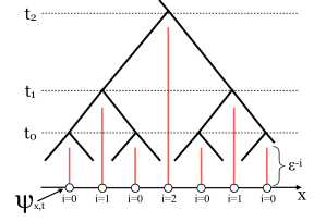
Figure 2: Depiction of the hierarchical set of barriers (red) of relative reflectivity $\epsilon^{-i}$ for $0<\epsilon<1$ and hierarchical index $i$ on a 1d-line, implemented by $\theta_{i}=\frac{\pi}{4}\epsilon^{i}$ for $0<\epsilon\leq 1$ in Eq. (4) for the quantum walk. These barriers generate an ultra-metrically arranged set of domains (tree) with a hierarchy of characteristic timescales $t_{i}$ for escape.

As a specific physical situation for such a setting, Ref. Boettcher (2020) considered a walk between two absorbing walls of separation $N=2^{l}+1$, equidistant from the starting site $x=2^{l-1}$. As the wall-sites $x=0$ and $x=2^{l}$ a fully absorbing, there is no flow reflecting out of those sites such that at the end of $l-1$ RG-steps, for either wall it is

$$\overline{\psi}_{\left\{0,2\right\}}=S_{l-1}^{\left\{A,B\right\}}\left({\cal C}_{l-1}^{-1}-S_{l-1}^{M}\right)^{-1}\psi_{IC}.$$ (15)

In Ref. Boettcher (2020), the RG calculation yielded for the quantum ultra-walk the walk dimension, as defined in Eq. (5):

$$d_{w}^{Q}=\frac{1}{2}+\frac{1}{2}\log_{2}\left(1+\epsilon^{-2}\right),$$ (16)

which grows without bound for decreasing $\epsilon$, i.e., for increasing barrier heights transports diminishes from ballistic ($d_{w}^{Q}=1$ for $\epsilon=1$) to extremely sub-diffusive for $\epsilon\to 0$. However, it was found numerically that, eventually, the entire weight of the wave function gets absorbed at arbitrarily distant walls for any finite value of $\epsilon$.

III Quantum Walks with Randomness

Ref. Vakulchyk et al. (2017) has investigated the behavior of DTQW on a 1d-line with coin parameters having extensive randomness, i.e., a different value for one of the variables $\theta$, $\vartheta$, or $\chi$ in Eq. (4) on every site $x$ (while the others were held fixed throughout). Unlike for the walk with regular hierarchical variation of $\theta$ according to Eq. (8) that we have described in Sec. II.3, it was shown there that such extensive randomness leads to a finite localization length for the walk at any level of randomness. For example, for $\vartheta=\chi=0$ in Eq. (4) Ref. Vakulchyk et al. (2017) selected at each site $x$ a random angle $\theta_{x}$ from a uniform probability distribution,

$$\mathcal{P}_{W}(\theta)=1/(2W),\qquad\frac{\pi}{4}-W\leq\theta\leq\frac{\pi}{4}+W,$$ (17)

with a adjustable disorder strength $0\leq W\leq\pi$ and centered such that each ${\cal C}_{x}$ becomes a Hadamard coin for vanishing randomness, $W\to 0$. It was found numerically that the DTQW localized for any non-zero value of $W$ considered there.

III.1 Quantum Ultra-Walk Model with Sub-extensive Randomness

Clearly, overlaying this form of extensive randomness with the hierarchical barriers analyzed in Sec. II.3, e.g. by replacing in Eq. (8) the constant $\theta_{0}$ with a random variable $\theta_{x}$ at each site $x$ in addition to the barrier strengths $\epsilon^{-i}$, merely enhances the already observed localization (see Fig. 4 below). In turn, it appears that the question regarding which level of sub-extensive randomness might be required to induce a localization transition is of some interest and can be conveniently studied in the context of such a one-dimensional quantum walk. To this end, specifically, we propose a simple two-parameter family of DTQW on the 1d-line with a combination of regular hierarchical barriers described by $\epsilon$ in combination with hierarchical randomness, manifested by choosing random angles $\theta_{i}$ from the $W$-controlled distribution in Eq. (17) merely for each level $i=i(x)$, as defined in Eq. (7). Indeed, we find evidence for localization transitions both for nontrivial values of $\epsilon$ for $W>0$ as well as of $W$ for $\epsilon<1$, while there is no transition either for $\epsilon=1$ at any value of $W$ or for $W=0$ at any $0<\epsilon\leq 1$ (the case considered in Ref. Boettcher (2020)). In light of the ability to treat this system with RG, see Sec. II.3, this will open the door for high-precision calculations via numerical iteration and disorder-averaging of the (exact) RG-recursion equations in the future.

Figure 3: Root mean square displacement $\sigma(t)$ for quantum ultra-walks with varying $\epsilon$ on a logarithmic scale. It shows how the increasing reflectivity in the hierarchy of barriers effects the transport behavior. According to Eq. (18), the slope of the curve for each $\epsilon$ corresponds to $1/d_{w}$, whose values match those predicted by the RG in Eq. (16) reasonably well for all but the smallest values of $\epsilon$.

III.2 Methods

Our means to determine the existence of those transitions in this study are very simple: For given $\epsilon$ and $W$, we generate multiple instances of placing random angles $\theta_{i}$ drawn from ${\cal P}_{W}$ in Eq. (17) into the coins on all sites $x$ (up to $\left|x\right|\leq L$ with $L=2^{16}$) matching Eq. (7) with that $i$ and any $\left|j\right|\leq L/2^{i+1}$. We note that each instance involves at most a sub-extensive, $O(\log L)$ choice of random angles $\theta_{i}$ that could ever be experienced by the walker while Ref. Vakulchyk et al. (2017) employed an extensive, $O(L)$ selection of random angles $\theta_{x}$. For each instance, we evolve DTQW initiated at $x=0$ for $t_{{\rm max}}=L=2^{16}$ time-steps to measure its mean-square displacement, $\sigma(t)^{2}$, which is the variance of $\rho(x,t)$ defined in Sec. II.1. It immediately follows from Eq. (5) that the root mean square displacement for large times $t$ scales as

$$\sigma(t)\sim t^{1/d_{w}},$$ (18)

from which we can extract the walk dimension $d_{w}$ asymptotically. In Fig. 3, we illustrate this procedure by reproducing the walk dimensions $d_{w}$ in Eq. (16) for various values of $\epsilon$ in the pure quantum ultra-walk without randomness ($W=0$). For any finite value of $d_{w}$ there is still extensive transport occurring, while $d_{w}=\infty$, or $1/d_{w}=0$, would indicate localization. In the quantum ultra-walk, there is no localization for any $\epsilon>0$, not even for any fraction of the wave function Boettcher (2020).

Since we are interested in the asymptotic behavior for large times and distances for the walk, we instead will plot our data for $\sigma(t)$ in form of an extrapolation plot. To this end, we convert $\sigma\sim At^{\frac{1}{d_{w}}}$ in Eq. (18) into

$$\frac{\log{\sigma(t)}}{\log{t}}\sim\frac{1}{d_{w}}+\frac{\log A}{\log{t}}.$$ (19)

When plotted with $X=1/\log t$ versus $Y=\frac{\log{\sigma(t)}}{\log{t}}$, asymptotically, Eq. (19) describes a line from which we can read off $1/d_{w}$ approximately at the intercept $X=0$, i.e., $t=\infty$. We first illustrate this technique in Fig. 4 for simulations employing extensive randomness which recap the findings of Ref. Vakulchyk et al. (2017) (for $\epsilon=1$) and show that localization only gets stronger for higher barriers ($\epsilon=0.6)$. Clearly, in all cases with $W>0$, the extrapolations indicate a vanishing of $1/d_{w}$, making $\sigma(t)$ bounded for large times $t$ as evidence that the walk remains localized.

Figure 4: Extrapolation plot for the root mean square displacement $\sigma(t)$ for a quantum walk with extensive randomness at various strengths $W$. Both for (a) $\epsilon=1$ and (b) $\epsilon=0.6$, any disorder with $W>0$ is sufficient to drive $1/d_{w}$ to zero asymptotically, as obtained by linear extrapolation (dashed lines) of each set of data at the intercept with the $Y$-axis. However, as the barriers in the system increase with decreasing $\epsilon$, the walker becomes more readily localized. Error bars are obtained from averaging over 25 instance for $\epsilon=1$ and from averaging over 20 instances for $\epsilon=0.6$.

III.3 Results

In the following, we apply the methods developed in Sec. III.2 to the model of a quantum ultra-walk with sub-extensive randomness introduced in Sec. III.1. In Fig. 5, we summarize our data of the walk simulations for various values in the ($\epsilon,W$)-plane. In particular, as shown in Fig. 5(a), for the otherwise homogeneous (barrier-free) 1d quantum walk obtained for $\epsilon=1$, the addition of merely sub-extensive randomness placed hierarchically on the lattice is insufficient to localize the walk for any value of $W$. Even for angles chosen entirely randomly ($W=\pi)$ the walk at most becomes mildly sub-diffusive and $1/d_{w}$ remains far from zero. This is in stark contrast with the corresponding case of extensive randomness Vakulchyk et al. (2017) shown in Fig. 4(a). However, in concert with the hierarchy of barrier that emerges for $\epsilon=0.8$ and $\epsilon=0.6$, as shown in Figs. 5(b,c), such a sub-extensive amount of randomness proves sufficient to induce localization. In fact, it appears that for each of those fixed values of $\epsilon<1$, there is a transition at a finite value of $W$, although it would be possible for that transition to be at $W=0$.

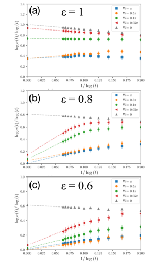
Figure 5: Extrapolation plots for the quantum ultra-walk model with various strengths $W$ of sub-extensive randomness at a fixed barrier strength of (a) $\epsilon=1$, (b) $\epsilon=0.8$, and (c) $\epsilon=0.6$. For $\epsilon=1$, the case of a homogeneous quantum walk, the addition of sub-extensive randomness of any strength $W$ is insufficient to bring $1/d_{w}$ even anywhere near to vanishing. For lower $\epsilon$, i.e., exponentially increasing barriers, some level of such randomness $W>0$ does prove sufficient to induce an apparent localization transition where there was none without $(W=0)$. Note that for lower $\epsilon$ (i.e., stronger barriers), the same amount of randomness suppresses transport more. Error bars were obtained by averaging over 50 instances.

We can summarize our results by sketching out a tentative phase diagram for the localization transition in the plane formed by the set of parameters $(\epsilon,W)$. In Fig. 6, we illustrate the emerging scenario, highlighting the region of localization ($1/d_{w}=0$, in red) from that of transport ($1/d_{w}>0$, in green) with a phase boundary between them estimated from our data. First, the earlier discussion in Sec. II.3 concerning the quantum ultra-walk without any randomness shows that the entire line ($\epsilon,W=0$) is not localized but that the line ($\epsilon=0,W$) for any $W$ certainly is. Thus, the phase boundary must pass the origin ($\epsilon=0,W=0$). While we can not entirely exclude the possibility that that boundary remains at $W=0$ also for most $\epsilon<1$, it is conceivable from Figs. 5(b,c) that for intermediate barrier strengths $\epsilon$ there is a transition at similarly intermediate values $W$, as the two interior marks at $\epsilon=0.6$ and $\epsilon=0.8$ insinuate. The argument for this scenario is strengthened by the fact that the point ($\epsilon=1,W=\pi$), yielding $1/d_{w}\approx 0.3-0.4$ from Fig. 5(a), appears far from localization and, thus, from the phase boundary. Hence, unless there is a discontinuous jump in $d_{w}$, that phase boundary seems to reach full randomness ($W=\pi$) at some value of $\epsilon_{c}$ that might be close to, but is well bounded-away from $\epsilon=1$, as indicated in Fig. 6. Then, either the phase boundary varies gradually between the origin and that point, as shown, or discontinuously jumps at $\epsilon_{c}$ from $W=0$ to $W=\pi$.

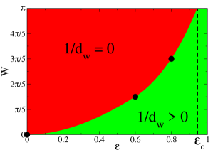
Figure 6: Sketch of the proposed phase diagram for the localization transition in the $(\epsilon,W)$-plane for the quantum ultra-walk model on a line with randomness. Eq. (18) suggests that walks with $1/d_{w}=0$ (red) become localized, while those with $1/d_{w}>0$ (green) maintain transport. The phase line is estimated based on the fact (1) that Eq. (16) provides $1/d_{w}>0$ for all $\epsilon>0$ without randomness ($W=0$) while $1/d_{w}=0$ at $\epsilon=0$, (2) that Figs. 5(b-c) show such a transition at intermediate values of $W$ for $\epsilon=0.6$ and $0.8$ (black dots), and (3) that Fig. 5(a) shows no transition for any $W$ when $\epsilon=1$. The strength of transport for $\epsilon=1$ even at maximum (sub-extensive) randomness, $W=\pi$, as apparent in Fig. 5(a), suggests that the localized domain terminates at some $\epsilon_{c}<1$.

IV Conclusions

Based on the recent solution of the quantum ultra-walk Boettcher (2020), a 1d DTQW that evolves through a spatially heterogeneous (albeit not random) environment characterized by a hierarchy of progressively diverging barriers (in the form of increasingly reflective quantum coins), we have extended this model by introducing a certain, sub-extensive amount of spatial randomness. The effect of extensive randomness, with random coin parameters on every site $x$, on a 1d DTQW has been well-studied and shown to lead to localization for even the smallest amount of randomness Vakulchyk et al. (2017). Our new model permitted us to explore the impact of sub-extensive randomness on localization as well as to trace out an interesting phase diagram with regions of localization and transport separated by a phase boundary, generated by the interplay of such randomness with the hierarchy of barriers. We have shown that, while each ineffective by themselves, such sparse randomness in combination with even mildly escalating barriers readily induces localization. While not yet resolved in great detail, the available evidence already suggests a few interesting features exhibited within that parameter space, with localization transitions occurring at either a non-trivial finite randomness or finite barrier strength, or both. Aside from the myriad applications of highly controllable DTQW in quantum algorithms Childs (2009); Childs et al. (2013), this model provides also a simple example with the potential for such a complex phase diagram. It would be interesting to supplement these studies with a similar continuous-time quantum walk Li and Boettcher (2017). While likely equivalent in most aspects Strauch (2006), we have favored a discrete-time formulation here, since the extra coin-space allows for richer designs in the walk dynamics.

In future work, we intend to employ RG to gain a more precise description of this diagram. While it is straightforward to obtain the exact RG-recursions from Eq. (12) that could be evolved numerically, replacing the regular progression of hierarchical barriers solved in Ref. Boettcher (2020) with a random sequence makes the prospect of receiving analytical results (even asymptotically) very daunting. Since contributions to the fixed points of the RG seem to arise from many poles Boettcher et al. (2017) throughout the complex-$z$ plane in Laplace space, originating in Eq. (2), even a numerical evolution of the RG-recursions does not yield insights easily. Alternatively, these questions should be more readily accessible using numerically the transfer matrix method of Ref. Vakulchyk et al. (2017).

Acknowledgements

This work is but a small contribution to acknowledge the tremendous impact that Bob Ziff, by strength of his kindness and intellect, has on all who know him and on the field of statistical physics.

References

- Inui et al. (2005) N. Inui, N. Konno, and E. Segawa, Phys. Rev. E 72, 056112 (2005).
- Falkner and Boettcher (2014) S. Falkner and S. Boettcher, Phys. Rev. A 90, 012307 (2014).
- Vakulchyk et al. (2017) I. Vakulchyk, M. V. Fistul, P. Qin, and S. Flach, Physical Review B 96, 144204 (2017).
- Crespi et al. (2013) A. Crespi, R. Osellame, R. Ramponi, V. Giovannetti, R. Fazio, L. Sansoni, F. D. Nicola, F. Sciarrino, and P. Mataloni, Nature Photonics 7, 322 (2013).
- Grossman et al. (2004) J. M. Grossman, D. Ciampini, M. D’Arcy, K. Helmerson, P. D. Lett, W. D. Phillips, A. Vaziri, and S. L. Rolston, in The 35th Meeting of the Division of Atomic, Molecular and Optical Physics, Tuscon, AZ, (DAMOP04) (2004).
- Karski et al. (2009) M. Karski, L. Forster, J.-M. Choi, A. Steffen, W. Alt, D. Meschede, and A. Widera, Science 325, 174 (2009).
- Manouchehri and Wang (2014) K. Manouchehri and J. Wang, Physical Implementation of Quantum Walks (Springer, Berlin, 2014).
- Perets et al. (2008) H. B. Perets, Y. Lahini, F. Pozzi, M. Sorel, R. Morandotti, and Y. Silberberg, Phys. Rev. Lett. 100, 170506 (2008).
- Peruzzo et al. (2010) A. Peruzzo, M. Lobino, J. C. F. Matthews, N. Matsuda, A. Politi, K. Poulios, X.-Q. Zhou, Y. Lahini, N. Ismail, K. Wörhoff, Y. Bromberg, Y. Silberberg, M. G. Thompson, and J. L. OBrien, Science 329, 1500 (2010).
- Preiss et al. (2015) P. M. Preiss, R. Ma, M. E. Tai, A. Lukin, M. Rispoli, P. Zupancic, Y. Lahini, R. Islam, and M. Greiner, Science 347, 1229 (2015).
- Qiang et al. (2016) X. Qiang, T. Loke, A. Montanaro, K. Aungskunsiri, X. Zhou, J. L. O’Brien, J. B. Wang, and J. C. F. Matthews, Nature Communications 7, 11511 (2016).
- Ryan et al. (2005) C. A. Ryan, M. Laforest, J. C. Boileau, and R. Laflamme, Phys. Rev. A 72, 062317 (2005).
- Sansoni et al. (2012) L. Sansoni, F. Sciarrino, G. Vallone, P. Mataloni, A. Crespi, R. Ramponi, and R. Osellame, Phys. Rev. Lett. 108, 010502 (2012).
- Schreiber et al. (2012) A. Schreiber, A. Gábris, P. P. Rohde, K. Laiho, M. Štefaňák, V. Potoček, C. Hamilton, I. Jex, and C. Silberhorn, Science 336, 55 (2012).
- Schreiber et al. (2011) A. Schreiber, K. N. Cassemiro, V. Potoček, A. Gábris, I. Jex, and C. Silberhorn, Phys. Rev. Lett. 106, 180403+ (2011).
- Tang et al. (2018) H. Tang, X.-F. Lin, Z. Feng, J.-Y. Chen, J. Gao, K. Sun, C.-Y. Wang, P.-C. Lai, X.-Y. Xu, Y. Wang, L.-F. Qiao, A.-L. Yang, and X.-M. Jin, Science Advances 4, 3174 (2018).
- Ramasesh et al. (2017) V. V. Ramasesh, E. Flurin, M. Rudner, I. Siddiqi, and N. Y. Yao, Phys. Rev. Lett. 118, 130501 (2017).
- Allés et al. (2012) B. Allés, S. Gündüç, and Y. Gündüç, Quantum Information Processing 11, 211-227 (2012).
- Asboth and Obuse (2013) J. K. Asboth and H. Obuse, Phys. Rev. B 88, 121406 (2013).
- Chakraborty et al. (2016) S. Chakraborty, L. Novo, A. Ambainis, and Y. Omar, Phys. Rev. Lett. 116, 100501 (2016).
- Childs (2009) A. M. Childs, Phys. Rev. Lett. 102, 180501 (2009).
- Childs et al. (2013) A. M. Childs, D. Gosset, and Z. Webb, Science 339, 791 (2013).
- S. and C.M. (2010) G. S. and C. C.M., J. Phys. A Math. Theor. 43, 235303 (2010).
- Kendon and Tregenna (2002) V. Kendon and B. Tregenna, in Quantum Communication, Measurement & Computing (QCMC’02), edited by J. H. Shapiro and O. Hirota (Rinton Press, 2002) p. 463.
- Kendon (2007) V. Kendon, Mathematical. Structures in Comp. Sci. 17, 1169 (2007).
- Kurzyński and Wójcik (2013) P. Kurzyński and A. Wójcik, Physical Review Letters 110, 200404 (2013).
- Lovett et al. (2010) N. B. Lovett, S. Cooper, M. Everitt, M. Trevers, and V. Kendon, Physical Review A 81, 042330+ (2010).
- Manouchehri and Wang (2008) K. Manouchehri and J. B. Wang, J. Phys. A: Math. Theor. 41, 065304 (2008).
- Obuse et al. (2015) H. Obuse, J. K. Asboth, Y. Nishimura, and N. Kawakami, Phys. Rev. B 92, 045424 (2015).
- Oliveira et al. (2006) A. C. Oliveira, R. Portugal, and R. Donangelo, Phys. Rev. A 74, 012312 (2006).
- Rudinger et al. (2013) K. Rudinger, J. K. Gamble, E. Bach, M. Friesen, R. Joynt, and S. N. Coppersmith, Journal of Computational and Theoretical Nanoscience 10, 1653 (2013).
- Shikano and Katsura (2010) Y. Shikano and H. Katsura, Phys. Rev. E 82, 031122 (2010).
- M. Stefanak et al. (2011) M. Stefanak, S.M. Barnett, B. Kollar, T. Kiss, and I. Jex, New J. Phys. 13, 033029 (2011).
- Ambainis (2007) A. Ambainis, SIAM J. Comput. 37, 210 (2007).
- Childs (2010) A. M. Childs, Communications in Mathematical Physics 294, 581 (2010), .
- Harrow et al. (2009) A. W. Harrow, A. Hassidim, and S. Lloyd, Physical Review Letters 103, (2009).
- Wiebe et al. (2012) N. Wiebe, D. Braun, and S. Lloyd, Physical Review Letters 109, (2012).
- Redner (2001) S. Redner, A Guide to First-Passage Processes (Cambridge University Press, Cambridge, 2001).
- Weiss (1994) G. H. Weiss, Aspects and Applications of the Random Walk (North-Holland, Amsterdam, 1994).
- Hughes (1996) B. D. Hughes, Random Walks and Random Environments (Oxford University Press, Oxford, 1996).
- Feller (1966) W. Feller, An Introduction to Probability Theory and its Applications, vol. I (John Wiley, New York London Sidney Toronto, 1966).
- Havlin and Ben-Avraham (1987) S. Havlin and D. Ben-Avraham, Adv. Phys. 36, 695 (1987).
- Ambainis (2003) A. Ambainis, International Journal of Quantum Information 1, 507 (2003).
- Ambainis et al. (2005) A. Ambainis, J. Kempe, and A. Rivosh, in Proceedings of the sixteenth annual ACM-SIAM symposium on Discrete algorithms, SODA ’05 (Society for Industrial and Applied Mathematics, Philadelphia, PA, USA, 2005) pp. 1099–1108.
- Boettcher et al. (2018) S. Boettcher, S. Li, T. D. Fernandes, and R. Portugal, Physical Review A 98, 012320 (2018).
- Plischke and Bergersen (1994) M. Plischke and B. Bergersen, Equilibrium Statistical Physics, 2nd edition (World Scientifc, Singapore, 1994).
- Boettcher et al. (2009) S. Boettcher, J. L. Cook, and R. M. Ziff, Physical Review E 80, 041115 (2009).
- Boettcher et al. (2012) S. Boettcher, V. Singh, and R. M. Ziff, Nature Communications 3, 787 (2012).
- Boettcher (2020) S. Boettcher, Physical Review Research 2, 023411 (2020).
- Grover (1997) L. K. Grover, Phys. Rev. Lett. 79, 325 (1997).
- Boettcher et al. (2014) S. Boettcher, S. Falkner, and R. Portugal, Physical Review A 90, 032324 (2014).
- Inui et al. (2004) N. Inui, Y. Konishi, and N. Konno, Physical Review A 69, 052323+ (2004).
- Inui and Konno (2005) N. Inui and N. Konno, Physica A 353, 333 (2005).
- Joye (2012) A. Joye, Quantum Information Processing 11, 1251 (2012).
- Ide et al. (2014) Y. Ide, N. Konno, E. Segawa, and X.-P. Xu, Entropy 16, 1501 (2014).
- Boettcher et al. (2017) S. Boettcher, S. Li, and R. Portugal, Journal of Physics A: Mathematical and Theoretical 50, 125302 (2017).
- Portugal (2013) R. Portugal, Quantum Walks and Search Algorithms (Springer, Berlin, 2013).
- Venegas-Andraca (2012) E. Venegas-Andraca, Quantum Information Processing 11, 1015 (2012).
- Portugal et al. (2015) R. Portugal, S. Boettcher, and S. Falkner, Physical Review A 91, 052319 (2015).
- Portugal (2016) R. Portugal, Quantum Information Processing 15, 1387 (2016).
- Bouchaud and Georges (1990) J.-P. Bouchaud and A. Georges, Phys. Rep. 195, 127 (1990).
- Grimmett et al. (2004) G. Grimmett, S. Janson, and P. F. Scudo, Physical Review E 69, 026119+ (2004).
- Konno (2002) N. Konno, Quantum Information Processing 1, 345 (2002).
- Segawa and Konno (2008) E. Segawa and N. Konno, Int. J. Quant. Inform. 6, 1231 (2008).
- Konno (2008) N. Konno, in Quantum Potential Theory, Lecture Notes in Mathematics, Vol. 1954, edited by U. Franz and M. Schürmann (Springer-Verlag: Heidelberg, Germany, 2008) pp. 309–452.
- Boettcher et al. (2013) S. Boettcher, S. Falkner, and R. Portugal, Journal of Physics: Conference Series 473, 012018 (2013).
- Boettcher et al. (2015) S. Boettcher, S. Falkner, and R. Portugal, Physical Review A 91, 052330 (2015).
- Konno (2005) N. Konno, J. Math. Soc. Japan 57, 1179 (2005).
- Boettcher and Li (2018) S. Boettcher and S. Li, Physical Review A 97, 012309 (2018).
- Childs et al. (2003) A. M. Childs, R. Cleve, E. Deotto, E. Farhi, S. Gutmann, and D. A. Spielman, in Proceedings of the Thirty-fifth Annual ACM Symposium on Theory of Computing, STOC ’03 (ACM, New York, NY, USA, 2003) pp. 59–68.
- Alexander and Orbach (1982) S. Alexander and R. Orbach, J. Physique Lett. 43, 625 (1982).
- Sinai (1982) Y. G. Sinai, Theory Probab. Appl. 27, 256 (1982).
- Brun et al. (2003) T. A. Brun, H. A. Carteret, and A. Ambainis, Phys. Rev. A 67, 052317 (2003).
- Konno (2009) N. Konno, Quantum Information Processing 8, 387 (2009).
- Ribeiro et al. (2004) P. Ribeiro, P. Milman, and R. Mosseri, Phys. Rev. Lett. 93, 190503 (2004).
- Teitel and Domany (1985) S. Teitel and E. Domany, Phys. Rev. Lett. 55, 2176 (1985).
- Ogielski and Stein (1985) A. T. Ogielski and D. L. Stein, Phys. Rev. Lett. 55, 1634 (1985).
- Huberman and Kerszberg (1985) B. Huberman and M. Kerszberg, J.Phys.A 18, L331 (1985).
- Maritan and Stella (1986) A. Maritan and A. Stella, J. Phys A: Math. Gen. 19, L269 (1986).
- Ceccatto et al. (1987) H. A. Ceccatto, W. P. Keirstead, and B. A. Huberman, Phys. Rev. A 36, 5509 (1987).
- Li and Boettcher (2017) S. Li and S. Boettcher, Physical Review A 95, 032301 (2017).
- Strauch (2006) F. W. Strauch, Phys. Rev. A 74, 030301 (2006).