Stochastic mRNA production by a three-state gene

Abstract

We consider a model of mRNA production governed by the dynamics of a gene that exists in three possible states – inactive, poised and active. The transitions between the adjacent states are controlled by stochastic processes characterized by corresponding on/off rates. mRNA is produced only when the gene is in active state and we also consider mRNA denaturation leading to its death. We derive the distribution of mRNA number and compare it to the known result for the two-state gene model.

1 Introduction

Consider a model of mRNA synthesis by a gene having three states – inactive (0), poised/paused/waiting (1) and active (2). mRNA translation takes place when the gene is in active state only and it degrades with a rate proportional to its concentration (number). Our approach extends the one used in [1] for a two-state gene that allows to compute the probability distribution of mRNA number as a function of the rates. An alternative way to describe gene state occupancy dynamics is based on explicit inclusion of the noise term into dynamical equations [2] which focused on the inflence of noise on the mRNA production.

The state of the system (gene + mRNA) is described by a two-dimensional integer vector $\{g,n\}$ where $g=0,1,2$ is the gene state and $n$ denotes a number of mRNA molecules. The transitions between gene states (shown in Fig.1) occur with the rates $k_{1\pm}$ for the pair inactive–poised and $k_{2\pm}$ for the pair poised–active while the direct transitions between inactive and active states are forbidden. The gene in active state produces a mRNA molecule with the rate $\nu$, these molecules degrade with the rate $\delta$.

Figure 1: The transitions in the three-state gene model.

All allowed transitions are described below. $\begin{array}[]{ll}\mbox{Transition}&\mbox{Rate}\\ \{0,n\}\to\{1,n\}&k_{1+}\\ \{0,n\}\to\{0,n-1\}&\delta n\\ &\\ \{1,n\}\to\{0,n\}&k_{1-}\\ \{1,n\}\to\{1,n-1\}&\delta n\\ \{1,n\}\to\{2,n\}&k_{2+}\\ &\\ \{2,n\}\to\{1,n\}&k_{2-}\\ \{2,n\}\to\{2,n-1\}&\delta n\\ \{2,n\}\to\{2,n+1\}&\nu\end{array}$

2 Balance equations

Using the above characterization of the transitions we can write down the dynamical equations for the probability $p_{g,n}(t)$ to have $n$ copies of mRNA for a gene in state $g$ at time $t$

$$p_{0,n}^{\prime}(t) = -k_{1+}p_{0,n}-n\delta p_{0,n}+(n+1)\delta p_{0,n+1}+k_{1-}p_{1,n},$$

$$p_{1,n}^{\prime}(t) = -k_{1-}p_{1,n}-n\delta p_{1,n}+(n+1)\delta p_{1,n+1}+k_{1+}p_{0,n}-k_{2+}p_{1,n}+k_{2-}p_{2,n},$$

$$p_{2,n}^{\prime}(t) = -k_{2-}p_{2,n}+k_{2+}p_{1,n}-n\delta p_{2,n}+(n+1)\delta p_{2,n+1}-\nu p_{2,n}+\nu p_{2,n-1}.$$

Rescaling the time variable $t\to t\delta$ and all rates $r\to r/\delta$ we obtain

$$p_{0,n}^{\prime}(t) = -k_{1+}p_{0,n}-np_{0,n}+(n+1)\delta p_{0,n+1}+k_{1-}p_{1,n},$$ (1)

$$p_{1,n}^{\prime}(t) = -k_{1-}p_{1,n}-np_{1,n}+(n+1)p_{1,n+1}+k_{1+}p_{0,n}-k_{2+}p_{1,n}+k_{2-}p_{2,n},$$

$$p_{2,n}^{\prime}(t) = -k_{2-}p_{2,n}+k_{2+}p_{1,n}-np_{2,n}+(n+1)p_{2,n+1}-\nu p_{2,n}+\nu p_{2,n-1}.$$

3 Generating functions

The probabilities $p_{i,n}(t)$ give rise to generating functions $G_{i}(z,t)$ defined as follows

$$G_{i}(z,t)=\sum_{n=0}^{\infty}z^{n}p_{i,n}(t).$$ (2)

Setting above $z=1$ we find

$$G_{i}(1,t)=\gamma_{i}=\sum_{n=0}^{\infty}p_{i,n}(t)$$

the probability of a gene to be in $i$-th state. The only observable of the model is the mRNA number $n$ at time $t$ defined by a probability $p_{n}=p_{0,n}+p_{1,n}+p_{2,n}$. The corresponding generating function reads

$$G(z,t)=G_{0}(z,t)+G_{1}(z,t)+G_{2}(z,t).$$

Note that

$$\partial G_{i}(z,t)/\partial z=\sum_{n=0}^{\infty}nz^{n-1}p_{i,n}(t)=\sum_{n=0}^{\infty}(n+1)z^{n}p_{i,n+1}(t),$$

leading to

$$\sum_{n=0}^{\infty}nz^{n}p_{i,n}(t)=z\;\partial G_{i}(z,t)/\partial z,$$

while (2) implies

$$\sum_{n=0}^{\infty}z^{n}p_{i,n-1}(t)=zG_{i}(z,t).$$

In order to derive equations for the generating functions we multiply each equation in (1) by $z^{n}$ and sum up w.r.t. $n$. This procedure leads to

$$\frac{\partial G_{0}(z,t)}{\partial t} = -k_{1+}G_{0}(z,t)+k_{1-}G_{1}(z,t)+(1-z)\frac{\partial G_{0}(z,t)}{\partial z},$$ (3)

$$\frac{\partial G_{1}(z,t)}{\partial t} = -k_{1-}G_{1}(z,t)+k_{1+}G_{0}(z,t)-k_{2+}G_{1}(z,t)+k_{2-}G_{2}(z,t)+(1-z)\frac{\partial G_{1}(z,t)}{\partial z},$$

$$\frac{\partial G_{2}(z,t)}{\partial t} = -k_{2-}G_{2}(z,t)+k_{2+}G_{1}(z,t)+(1-z)\frac{\partial G_{2}(z,t)}{\partial z}-\nu(1-z)\frac{\partial G_{2}(z,t)}{\partial z}.$$

The natural assumption in the model is that at $t=0$ the gene is inactive ($i=0$) and the number of mRNA molecules $n=0$, so that the initial conditions read $p_{0,0}(0)=1$ and we find $G_{i}(z,0)=\delta_{i,0}$. Adding up the equations in (3) we obtain

$$\frac{\partial G(z,t)}{\partial t}=(1-z)\left[\frac{\partial G(z,t)}{\partial z}-\nu\frac{\partial G(z,t)}{\partial z}\right].$$ (4)

4 Steady state equations

Analytical solution of (3) that completely determines the dynamics of the mRNA is not known. We consider an asymptotic behavior of the probability $p_{i,n}$ at large times $t\to\infty$. Then the equations (3) turn into a system of ODEs

$$k_{1-}G_{1}(z)-k_{1+}G_{0}(z)+(1-z)G_{0}^{\prime}(z)=0,$$ (5)

$$k_{1+}G_{0}(z)-k_{1-}G_{1}(z)-k_{2+}G_{1}(z)+k_{2-}G_{2}(z)+(1-z)G_{1}^{\prime}(z)=0,$$ (6)

$$k_{2+}G_{1}(z)-k_{2-}G_{2}(z)+(1-z)G_{2}^{\prime}(z)-\nu(1-z)G_{2}^{\prime}(z)=0.$$ (7)

Adding up these equations we obtain a relation

$$\sum_{i=0}^{2}G_{i}^{\prime}(z)=G^{\prime}(z)=\nu G_{2}(z).$$ (8)

In order to find the asymptotic values of $\gamma_{i}$ set $z=1$ in (5-7) and obtain

$$k_{1-}\gamma_{1}-k_{1+}\gamma_{0}=0,$$

$$k_{1+}\gamma_{0}-k_{1-}\gamma_{1}-k_{2+}\gamma_{1}+k_{2-}\gamma_{2}=0,$$

$$k_{2+}\gamma_{1}-k_{2-}\gamma_{2}=0,$$

where $\gamma_{0}+\gamma_{1}+\gamma_{2}=1$ to produce

$$\gamma_{0}=k_{1-}k_{2-}/K,\quad\gamma_{2}=k_{1+}k_{2+}/K,\quad K=k_{1-}k_{2-}+k_{1+}k_{2-}+k_{1+}k_{2+}.$$ (9)

5 Solution for $G_{2}(z)$

It follows from (8) that in order to find $G(z)$ and determine the observable probability $p_{n}$ it is suffice to have an explicit expression for $G_{2}(z)$. In this section we first reduce the system (5-7) to a single equation for $G_{2}(z)$ and then obtain its solution.

5.1 Reduction to a single equation

First eliminate $G_{1}$ from (5,7) to produce

$$k_{1-}[(k_{2-}+\nu(1-z))G_{2}-(1-z)G_{2}^{\prime}]=k_{2+}[k_{1+}G_{0}-(1-z)G_{0}^{\prime}].$$ (10)

Differentiate (5) w.r.t. $z$ and substitute into the result $G_{1}^{\prime}(z)$ from (8)

$$(1-z)G_{0}^{\prime\prime}-(1+k_{1+})G_{0}^{\prime}+k_{1-}(\nu G_{2}-G_{0}^{\prime}-G_{2}^{\prime})=0.$$

Now use this relation together with (10) to obtain

$$(1-z)(G_{2}^{\prime\prime}-\nu G_{2}^{\prime})-(1+k_{2-}+k_{2+})G_{2}^{\prime}+\nu(1+k_{2+})G_{2}=k_{2+}G_{0}^{\prime}.$$ (11)

Similarly differentiate (7) w.r.t. $z$ and substitute $G_{1}^{\prime}(z)$ to produce

$$(1-z)[G_{2}^{\prime}-\nu G_{2}^{\prime}]^{\prime}-(1+k_{2-}G_{2}^{\prime})+\nu G_{2}+k_{2+}(\nu G_{2}-G_{0}^{\prime}-G_{2}^{\prime})=0.$$

Use it again with (10) to generate

$$-(1-z)G_{0}^{\prime\prime}-(1+k_{1-}+k_{1+})G_{0}^{\prime}=k_{1-}(\nu G_{2}-g_{2}^{\prime}).$$ (12)

Finally, express $G_{0}^{\prime}$ from (11) and use it in (11) to construct a single third order differential equation for $G_{2}$

$$(z-1)^{2}G_{2}^{\prime\prime\prime}+(z-1)(3+\kappa_{1}-\nu(z-1))G_{2}^{\prime\prime}-\nu\kappa_{3}G_{2}$$ (13)

$$+ [\kappa_{3}+(1+k_{1-}+k_{1+})k_{2-}-\nu(z-1)(3+\kappa_{2})]G_{2}^{\prime}=0,$$

where

$$\kappa_{1}=k_{1-}+k_{1+}+k_{2-}+k_{2+},\kappa_{2}=\kappa_{1}-k_{2-},\kappa_{3}=k_{1-}+(1+k_{1+})(1+k_{2+}).$$

5.2 Expression for $G_{2}(z)$

The solution of the linear ODE (13) was obtained with computer algebra software Mathematica, it has three components, but only one of these three does not diverge at $z=1$. This component is a generalized hypergeometric function

$$G_{2}(z)=c\;{}_{2}F_{2}(\{1+K_{2-},1+K_{2+}\},\{1+K_{1-},1+K_{1+}\},\nu(z-1)),$$

where $c$ is the undetermined constant and we introduce the shortcut notations

$$K_{1\pm}=(\kappa_{1}\pm\sqrt{\kappa_{1}^{2}-4\kappa_{0}})/2,\quad K_{2\pm}=(\kappa_{2}\pm\sqrt{\kappa_{2}^{2}-4k_{1+}k_{2+}})/2,$$

where $\kappa_{0}=(k_{1-}+k_{1+})k_{2-}+k_{1+}k_{2+}$. Note that $K_{i\pm}$ are homogeneous functions of degree one.

The constant $c$ is selected to satisfy the condition $G_{2}(1)=\gamma_{2}$. As ${}_{2}F_{2}(\{a_{1},a_{2}\},\{b_{1},b_{2}\},0)=1$ we immediately find that $c=\gamma_{2}=k_{1+}k_{2+}/(k_{1-}k_{2-}+k_{1+}k_{2-}+k_{1+}k_{2+})$. Thus we finally find

$$G_{2}(z)=\frac{{}_{2}F_{2}(\{1+K_{2-},1+K_{2+}\},\{1+K_{1-},1+K_{1+}\},\nu(z-1))}{1+(1+k_{1-}/k_{1+})(k_{2-}/k_{2+})}.$$ (14)

6 Computation of $G(z)$

Relation (8) allows to find $G(z)$ as an integral

$$G(z)=\nu\int G_{2}(z)dz,$$

provided $G(1)=1$. The generalized hypergeometric functions ${}_{p}F_{q}({\bf a},{\bf b},x)$, where ${\bf a}=\{a_{1},a_{2},\ldots,a_{p}\}$ and ${\bf b}=\{b_{1},b_{2},\ldots,b_{q}\}$ are the vectors of $p$ and $q$ components respectively, have a nice property that both derivatives and integrals are expressed through the same functions [3]. Specifically,

$$\int{}_{p}F_{q}({\bf a},{\bf b},x)dx=\frac{\pi({\bf b}-1)}{\pi({\bf a}-1)}\;{}_{p}F_{q}({\bf a}-1,{\bf b}-1,x),$$

where we employ the following notations for a $p$-dimensional vector ${\bf v}$

$$\pi({\bf v})=\prod_{i=1}^{p}v_{i},\quad{\bf v}+m=\{v_{1}+m,v_{2}+m,\ldots,v_{p}+m\}.$$

Introducing $x=\nu(z-1)$ we find

$$\nu\int{}_{p}F_{q}({\bf a},{\bf b},\nu(z-1))dz=\int{}_{p}F_{q}({\bf a},{\bf b},x)dx,$$

so that

$$G(z)={}_{2}F_{2}(\{K_{2-},K_{2+}\},\{K_{1-},K_{1+}\},\nu(z-1)),\quad G(1)=1.$$ (15)

7 Steady state mRNA distribution

From the definition of the generating function we have

$$G(z)=\sum_{n=0}^{\infty}z^{n}p_{n},$$

leading to a conclusion that $p_{n}$ is the coefficient in the Taylor expansion of $G(z)$ around $z=0$. The explicit expression for $p_{n}$ then reads [4]

$$p_{n} = \frac{r_{n}(K_{2-})r_{n}(K_{2+})}{r_{n}(K_{1-})r_{n}(K_{1+})}\cdot\frac{\nu^{n}}{n!}\cdot\;{}_{2}F_{2}(\{K_{2-},K_{2+}\}+n,\{K_{1-},K_{1+}\}+n,-\nu),$$

$$r_{n}(x) = \Gamma(x+n)/\Gamma(x),$$ (16)

where $r_{n}(x)$ is the Pochhammer symbol defined via gamma function $\Gamma(x)$.

Note that for $x\sim O(1)$ and large $n\gg 1$ the value of $r_{n}(x)$ grows as $r_{n}(x)\sim x^{n}$ so that the first factor in (16) behaves as $(K_{2-}K_{2+})^{n}/(K_{1-}K_{1+})^{n}$.

7.1 Reduction and comparison to two-state gene model

To reduce the three-state model to two-state one we set $k_{1-}=0$ so that $\gamma_{0}=0$ and the gene can be only in the active (2) or the poised (1) state which effectively plays a role of the inactive state. In this case $p_{0,n}=0,\;G_{0}(z)=0$ and we end up with the following system of equations

$$-k_{2+}G_{1}(z)+k_{2-}G_{2}(z)+(1-z)G_{1}^{\prime}(z)=0,$$ (17)

$$k_{2+}G_{1}(z)-k_{2-}G_{2}(z)+(1-z)G_{2}^{\prime}(z)-\nu(1-z)G_{2}^{\prime}(z)=0.$$ (18)

The model (17,18) was discussed in [1] and in this case the probability $p_{n}$ reads

$$p_{n}=\frac{\nu^{n}r_{n}(K_{+})}{n!r_{n}(K_{+}+K_{-})}\;{}_{1}F_{1}(\{K_{+}+n\},\{K_{+}+K_{-}+n\},-\nu),$$ (19)

where $K_{\pm}=k_{2\pm}$. This result can be also obtained directly from (16). We find for $k_{1-}=0$ the values of $\kappa_{0}=k_{1+}(k_{2-}+k_{2+}),\ \kappa_{1}=k_{1+}+k_{2+}+k_{2-},\ \kappa_{2}=k_{1+}+k_{2+}$ to compute $K_{1\pm}=(k_{1+}+k_{2+}+k_{2-}\pm(k_{1+}-k_{2+}-k_{2-}))/2$ and $K_{2\pm}=(k_{1+}+k_{2+}\pm(k_{1+}-k_{2+}))/2$. It leads to $K_{1-}=K_{2+}=k_{1+}$ and $K_{1+}=k_{2+}+k_{2-}=K_{+}+K_{-},\ K_{2-}=k_{2+}=K_{+}$ so that the property of the hypergeometric function

$${}_{p+1}F_{q+1}(\{a_{1},a_{2},\ldots,a_{p},c\},\{b_{1},b_{2},\ldots,b_{q},c\},x)={}_{p}F_{q}(\{a_{1},a_{2},\ldots,a_{p}\},\{b_{1},b_{2},\ldots,b_{q}\},x)$$

implies

$${}_{2}F_{2}(\{K_{2-},K_{2+}\}+n,\{K_{1-},K_{1+}\}+n,-\nu)={}_{1}F_{1}(\{K_{+}+n\},\{K_{+}+K_{-}+n\},-\nu).$$

7.2 Qualitative model predictions

When $k_{1-}\ll k_{1+}$ one expects that $p_{n}$ for three-state gene should be quite close to the two-state gene solution. The numerical simulations confirm the assumption (Fig. 2a). When $k_{1-}$ increases the population of the inactive state according to (9) also grows thus reducing simultaneously the active state probability. As expected this reduction results in the shift to the cells expressing lower mRNA numbers (Fig. 2b).

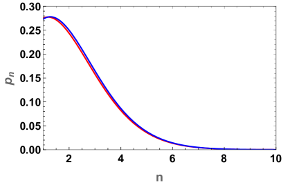
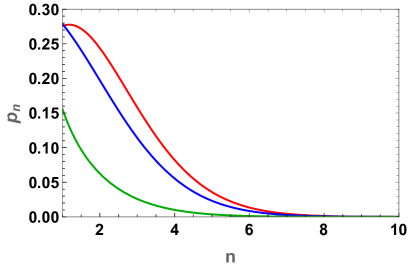
(a)	(b)

Figure 2: (a) The two-state (blue) and three-state (red) gene model mRNA distributions for $k_{1-}\ll k_{1+}$ demonstrate nearly perfect coincidence. The parameter values are $k_{1-}=0.13,\;k_{1+}=1.3,\;k_{2-}=2.3,\;k_{2+}=4.2,\;\nu=3$ for the three-state and $k_{-}=2.3,\;k_{+}=4.2,\;\nu=3$ for the two-state gene model. (b) An effect of the inactive state population on mRNA production in three-state gene model. The parameters are $k_{1+}=1.3,\;k_{2-}=2.3,\;k_{2+}=4.2,\;\nu=3$ with $k_{1-}$ equal to $0.13$ (red), $1.3$ (blue) and $13.0$ (green) respectively.

8 Hypergeometric function asymptotic expansion for large argument

The $p_{n}$ expressions (19) and (16) for two- and three-state model respectively might need to be evaluated when both the argument $\nu$ and the parameters of hypergeometric function are large. In this case it is worth to use asymptotic expansion for fast and accurate computation of these functions ${}_{k}F_{k},\;k=1,2$.

8.1 Asymptotics of ${}_{1}F_{1}$

We use asymptotics at large $|z|\to\infty$

$${}_{1}F_{1}(\{a\},\{b\},z)\sim\left\{\begin{array}[]{ccc}(-z)^{-a}\Gamma(b){}_{2}F_{0}(\{a,a-b+1\},\{\},-1/z)/\Gamma(b-a),&&a,b<|z|,\\ z^{a-b}e^{z}\Gamma(b){}_{2}F_{0}(\{b-a,1-a\},\{\},1/z)/\Gamma(a),&&a,b\geq|z|,\end{array}\right.$$ (20)

where the function ${}_{2}F_{0}(\{a,b\},\{\},x)$ is computed through the series

$${}_{2}F_{0}(\{a,b\},\{\},x)=\sum_{k=0}^{\infty}r_{k}(a)r_{k}(b)x^{k}/k!,$$

as a particular case of the general definition

$${}_{p}F_{q}(\{a_{1},a_{2},\ldots,a_{p}\},\{b_{1},b_{2},\ldots,b_{q}\},x)=\sum_{k=0}^{\infty}\frac{\prod_{i=1}^{p}r_{k}(a_{i})}{\prod_{j=1}^{q}r_{k}(b_{j})}\cdot\frac{x^{k}}{k!},$$ (21)

where the upper limit in the sum is replaced by positive integer $m$ representing number of terms in the expansion. Note that (19) for $K_{\pm}\sim O(1)$ at large $\nu\gg 1$ and $n<\nu$ one has to use the first formula in (20) while for large $n>\nu$ the second line is employed.

8.2 Asymptotics of ${}_{2}F_{2}$

When $|z|\gg 1$ we employ the following asymptotic formula [5]

$${}_{2}F_{2}(\{a_{1},a_{2}\},\{b_{1},b_{2}\},z)\sim\left\{\begin{array}[]{lc}(-z)^{-a_{1}}\frac{\Gamma(b_{1})\Gamma(b_{2})\Gamma(a_{2}-a_{1})}{\Gamma(a_{2})\Gamma(b_{1}-a_{1})\Gamma(b_{2}-a_{1})}&\\ \times{}_{3}F_{1}(\{a_{1},a_{1}-b_{1}+1,a_{1}-b_{2}+1\},\{a_{1}-a_{2}+1\},-1/z)&\\ +(-z)^{-a_{2}}\frac{\Gamma(b_{1})\Gamma(b_{2})\Gamma(a_{1}-a_{2})}{\Gamma(a_{1})\Gamma(b_{1}-a_{2})\Gamma(b_{2}-a_{2})}&\\ \times{}_{3}F_{1}(\{a_{2},a_{2}-b_{1}+1,a_{2}-b_{2}+1\},\{a_{2}-a_{1}+1\},-1/z),&a_{i},b_{i}<|z|,\\ e^{z}z^{A_{2}-B_{2}}\frac{\Gamma(b_{1})\Gamma(b_{2})}{\Gamma(a_{1})\Gamma(a_{2})}\sum_{k=0}^{\infty}c_{k}(1/z)^{k},&a_{i},b_{i}\geq|z|,\end{array}\right.$$ (27)

where the upper limit in the last line sum is replaced by positive integer $m$ . We use the notation $A_{2}=a_{1}+a_{2},\;B_{2}=b_{1}+b_{2}$ and the expansion coefficients $c_{k}$ are defined by a recursion

$$c_{0}=1,\ c_{1}=(A_{2}-1)(A_{2}-B_{2})+b_{1}b_{2}-a_{1}a_{2},\$$

$$kc_{k}=(1-B_{2}+a_{1}(2+a_{1})+a_{2}(2+a_{2})-A_{2}B_{2}+a_{1}a_{2}+b_{1}b_{2}+(2B_{2}-3(A_{2}+1))k+2k^{2})c_{k-1}$$

$$-(k-A_{2}+b_{1}-1)(k-A_{2}+b_{2}-1)(k-A_{2}+B_{2}-2)c_{k-2}.$$ (28)

References

• [1] J. Pessoud, B. Ycart, Markovian modelling of gene product synthesis, Theor. Population Bio. 48, 222-234 (1995).
• [2] G. Rieckh, G. TkacΜ†ik, Noise and information transmission in promoters with multiple internal states, Biophys. J. 106, 1194-1204 (2014).
• [3] https://functions.wolfram.com/HypergeometricFunctions/Hypergeometric2F2/21/01/01/
• [4] https://functions.wolfram.com/HypergeometricFunctions/Hypergeometric2F2/06/01/02/01/01/
• [5] https://functions.wolfram.com/HypergeometricFunctions/Hypergeometric2F2/06/02/02/
• [6] https://functions.wolfram.com/HypergeometricFunctions/Hypergeometric1F1/06/02/