IL-flOw: Imitation Learning from Observation using Normalizing Flows

Abstract

We present an algorithm for Inverse Reinforcement Learning (IRL) from expert state observations only. Our approach decouples reward modelling from policy learning, unlike state-of-the-art adversarial methods which require updating the reward model during policy search and are known to be unstable and difficult to optimize. Our method, IL-flOw, recovers the expert policy by modelling state-state transitions, by generating rewards using deep density estimators trained on the demonstration trajectories, avoiding the instability issues of adversarial methods. We demonstrate that using the state transition log-probability density as a reward signal for forward reinforcement learning translates to matching the trajectory distribution of the expert demonstrations, and experimentally show good recovery of the true reward signal as well as state of the art results for imitation from observation on locomotion and robotic continuous control tasks.

1 Introduction

Imitation learning (IL) is an effective class of algorithms for designing and optimizing controllers for robot systems. While recent advances in Reinforcement Learning have shown it is capable of producing agents that learn robot controllers from scratch, IL remains a more practical alternative for cases where it is easier to specify robot behaviours through examples than through rewards. We take an approach similar to existing work [1, 2] on learning from demonstrations (LfD). We use expert data to build a reward model to be maximized with existing RL algorithms. Unlike LfD, where an expert demonstrates which actions to perform at some robot states, we focus on the case where action supervision is not available: the agent only gets access to a dataset of state/observations sequences – a setting known as Imitation Learning from Observations (ILfO). While LfD usually requires providing demonstrations by teleoperation of the robot, ILfO aims to utilize streams of state and observational data, much like a human can learn to do a task by watching other people.

We formulate the problem of learning from observations as a distribution matching problem: we want to find the policy parameters that result in observation sequences that are similar to those in a dataset of expert demonstrations. This is similar to recent work [2, 3, 4] that uses adversarial optimization. Our approach differs in that we fit a density model on expert observation sequences, which we then use to produce rewards for policy search with RL optimizers, decoupling the policy optimization from the reward learning processes. To the best of our knowledge the closest approaches to ours are [5] where they also use neural density estimators although for occupancy measure estimation and address state-action imitation instead of state-only. Their formulation requires a discounted infinite horizon agent however, as opposed to our undiscounted finite horizon RL optimization. And [6], which also addresses the lack of smoothness of the KL-divergence objectives, by opting to minimize Wasserstein distance however instead of noise-expanded distributions, although unlike ours their reward signal is non-stationary. Our imitation signal is non-adversarial, stationary and reusable for downstream tasks.

2 Background

We formulate our task by an MDP $(\mathcal{S},\mathcal{A},\mathcal{P},r,p_{0})$ where $\mathcal{S}$ is the state space, $\mathcal{A}$ is the action space, $\mathcal{P}:\mathcal{S}\times\mathcal{A}\times\mathcal{S}\rightarrow[0,1]$ is the transition dynamics, $r:\mathcal{S}\times\mathcal{A}\rightarrow\mathbb{R}$ is the reward function, $p_{0}:\mathcal{S}\rightarrow[0,1]$ is the initial state distribution. We define a policy $\pi:\mathcal{S}\times\mathcal{A}\rightarrow[0,1]$. The probability of a trajectory $\tau=\{s_{0:T},a_{0:T}\}$ of $T+1$ states and actions when following the policy $\pi$ is given by: $p_{\pi}(s_{0:T},a_{0:T})=p_{0}(s_{0})\prod_{t=0}^{T-1}p(s_{t+1}|s_{t},a_{t})\pi(a_{t}|s_{t})$. If we are interested in state-only trajectories, then we must consider transitions over states, with the effects of the policy integrated out: $p_{\pi}(s_{t+1}|s_{t})=\int p(s_{t+1}|s_{t},a)\pi(a|s_{t})\mathrm{d}a$. It follows that the two quantities of interest are the probability of a trajectory over states

$$\text{given a policy }\pi:p_{\pi}(s_{0:T-1})=p_{0}(s_{0})\textstyle\prod_{t=0}^{T-1}p_{\pi}(s_{t+1}|s_{t}),$$ (1)

$$\text{and given an expert }E:p_{E}(s_{0:T-1})=p_{0}(s_{0})\textstyle\prod_{t=0}^{T-1}p_{E}(s_{t+1}|s_{t}),$$ (2)

where state imitation learning from observations occurs by distribution fitting $p_{\pi}$ to match $p_{E}$.

3 IL-flOw

In this section we derive IL-flOw, an Imitation Learning from Observation algorithm that implements trajectory matching by maximizing the log probability of the expert transitions. We begin by reformulating the reverse KL objective as an expression over individual transitions. This suggests a straightforward approach in which we use an approximation of the log probability of expert transitions as a reward signal alongside entropy maximization. Secondly, we present our noise regularization approach for density estimation of expert transitions using normalizing flows.

3.1 Imitation Learning via a Trajectory Matching Objective

Given our objective is matching the distribution of trajectories $p_{\pi}$ induced by our current policy $\pi$, and the distribution $p_{E}$ by some expert $E$, in this section we reformulate the reverse KL (RKL) divergence such that it is more amenable for use in a reinforcement learning context.

First, consider the RKL between trajectory distributions:

$$D_{\text{KL}}\left(p_{\pi}||p_{E}\right) =-\mathbb{E}_{s_{0:T-1}\sim p_{\pi}}\left[\sum_{t=0}^{T-1}\log p_{E}(s_{t+1}|s_{t})\right]+\mathbb{E}_{s_{0:T-1}\sim p_{\pi}}\left[\sum_{t=0}^{T-1}\log p_{\pi}(s_{t+1}|s_{t})\right]$$ (3)

The first term is the likelihood of policy samples under the expert distribution. The second term corresponds to the entropy of the state-sequence distribution induced by the policy. Note that, by the law of iterated expectations, the second term can be written as the expectation of the per-timestep transition entropies (full derivation in Appendix B)

$$\mathcal{H}(p_{\pi})=-\mathbb{E}_{s_{0:T-1}\sim p_{\pi}}\left[\sum_{t=0}^{T-1}\log p_{\pi}(s_{t+1}|s_{t})\right]=\mathbb{E}_{s_{0:T-1}\sim p_{\pi}}\left[\sum_{t=0}^{T-1}\mathcal{H}\left(p_{\pi}(\cdot|s_{t})\right)\right].$$ (4)

If we assume the dynamics are deterministic and invertible, we can simplify the expression further by using the change of variables formula to express the state sequence entropy in terms of the policy (full derivation in Appendix B)

$$\mathcal{H}\left(p_{\pi}(\cdot|s_{t})\right) =-\int p_{\pi}(s_{t+1}|s_{t})\log p_{\pi}(s_{t+1}|s_{t})\mathrm{d}s_{t+1}\approx\mathcal{H}\left(\pi(\cdot|s_{t})\right).$$ (5)

While the assumption of invertible dynamics is restrictive, our experiments show that it is a useful approximation for robotics tasks. Minimizing the KL divergence objective above is equivalent to maximizing the following objective:

$$J(\pi)+\mathcal{H}(p_{\pi}) \approx\mathbb{E}_{\tau\sim p_{\pi}(\tau)}\left[\sum_{t=0}^{T-1}\log p_{E}(s_{t+1}|s_{t})+\sum_{t=0}^{T-1}\mathcal{H}(\pi(\cdot|s_{t}))\right].$$ (6)

This objective can be optimized with RL algorithms by setting rewards to $r_{t}=\log p_{E}(s_{t+1}|s_{t})$ and maximizing the undiscounted return, while penalizing the negative entropy of the policy. This suggests a practical algorithm where we can use a finite horizon variant of Soft Actor-Critic [7], which maximizes a reward signal alongside the entropy of the policy.

3.2 Noise Conditioned Normalizing Flows

Our approach requires fitting a model of $p_{E}(s_{t+1}|s_{t})$, using a dataset of demonstrations $D_{E}$. We use a normalizing flow model to fit $p_{E}$, a very powerful and expressive type of density estimator. While well-suited for our purpose, these models are known to overfit with little data, leading to poor out of distribution generalization [8, 9]. Since we aim to use this density model as a reward model for an RL optimizer, we also want it to be suitable for policy optimization. This means producing reasonably low probabilities for observations that are far from the expert data and likely encountered during policy optimization, while resulting in a smooth optimization landscape. Given that $D_{E}$ only covers a subset of all possible behaviours that could be encountered during optimization, we have little control on the predicted log-probability density for non-expert behaviour. This results in a noisy, and possibly biased signal for policy optimization outside the support of the training dataset.

To address the issues above, we fit a set of noise conditioned distributions, $\tilde{p}_{E}(s_{t+1}|s_{t},h)$ where $h\sim\mathrm{Uniform}\left[0,h_{max}\right]$ represents the noise level – the magnitude of zero-mean noise added to the training data. At training time, we draw a noise level $h$ and two zero-mean noise samples $\bm{\epsilon_{s}}$ and $\bm{\epsilon_{s^{\prime}}}$ for each expert transition $(\bm{s_{E}},\bm{s_{E}^{\prime}})$. We set $\bm{\tilde{s}_{E}}\leftarrow\bm{s_{E}}+\bm{h\epsilon_{s}}$ and $\bm{\tilde{s}_{E}^{\prime}}\leftarrow\bm{s_{E}^{\prime}}+\bm{h\epsilon_{s^{\prime}}}$ and fit our model to maximize $\log p(\bm{\tilde{s}_{E}^{\prime}}|\bm{\tilde{s}_{E}},h)$. At test time, with $h=0$ we recover the noise-free fitted distribution $\tilde{p}_{E}$, while with $h=h_{max}$ we get a distribution closer in shape to the distribution of the additive noise, as it then dominates over $p_{E}$. Any intermediate value for $h$ smoothly interpolates between the two. Since the sampled noise is zero-mean, transitions close to the dataset $D_{E}$ will have the highest log-probability, irrespective of the noise level, providing a signal with tunable smoothness that is useful for policy search. In Appendix 3 we show an example of varying the noise level $h$. Noise regularization for density estimators has been studied in [15], and noise-conditioned normalizing flows have previously been applied to 3D data [16]. Previous work restricts the noise level to $h\approx 0$ at test time however, while we actively use the set of noise levels $h\in[h_{min},h_{max}]$ to control the smoothness of our optimization objective, giving the agent a usable signal at all times during policy optimization.

In the results below, we chose to use Neural Spline Flows [17] for density estimation and Soft Actor-Critic [7] as the policy optimizer, but our objective and approach are applicable to any combination of a density estimator and optimizer.

3.3 Soft Actor-Critic in time-limited MDPs and adaptive noise conditioning

Operating in a finite horizon setting, we augment the state with a time-to-horizon variable $t_{H}$, representing the number of timesteps to go in an episode, therefore making the actor and critic networks both time-aware. We also augment the action by one additional dimension representing the noise level $h$ at which to sample our density function, thus letting the agent interact with the entirety of the log probability reward signal. We know however that the highest log density is achieved by the training dataset, at the noise-free level $h_{min}=0$. The agent should learn to choose a low value of $h$ when close to the expert, while as we move away from the expert support the appropriate value of $h$ smoothly increases, expanding the support of the density function.

4 Experiments and Results

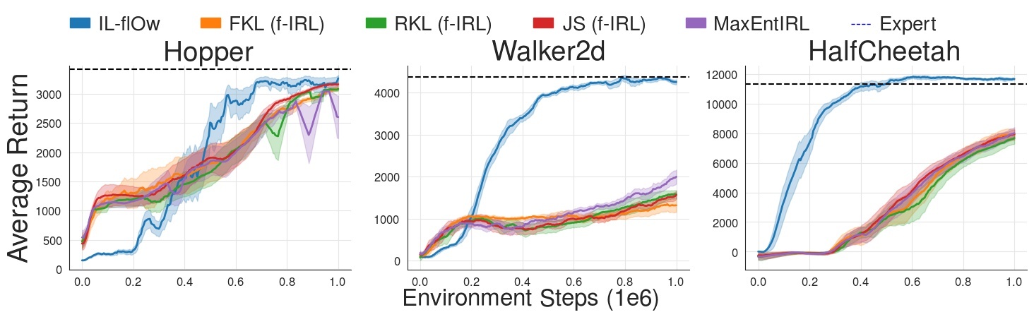
Figure 1: Learning curves for IL-flOw and 4 other baselines: f-IRL (FKL, RKL, JS), and MaxEntIRL with 40 expert demonstrations across 3 random seeds. The shaded area represents half a standard deviation.

We collect $n=150$ demonstration trajectories on three Mujoco [18] simulated environments: Hopper-v2, Walker2d-v2, and HalfCheetah-v2, using a SAC expert trained for 1M timestep, using $n$ random seeds. To evaluate the performance with varying amounts of demonstrations, we use a subset of 40, 20 or 10 trajectories (respectively $(40,20,10)\cdot 10^{3}$ data points) as the training dataset $D_{expert}$ for the density estimator. We compare IL-flOw to the three variants of the f-IRL [4] algorithm, as well as a state only version of MaxEnt IRL [1], using the implementations provided by [4]. MaxEnt IRL minimizes forward KL divergence in trajectory space under the maximum entropy RL framework. f-IRL is an imitation learning from observation algorithm that operates by state marginal distribution matching, through optimization of the analytical gradient of any f-divergence (JS, FKL, RKL). It also learns a stationary reward that is reusable, although the imitation agent still faces a moving reward function in training through their iterative training process, while for IL-flOw the reward learning and the RL process are sequential, to convergence.

We report our results in Table 1 and Figure 1. IL-flOw outperforms all the baselines on all three studied environments, even with limited amounts of expert demonstrations. Notably it learns much faster than baseline algorithms. Figure 2 shows the relationship between the learnt reward signal and the environment reward. Our reward function is positively correlated with the environment reward and increases monotonically as we get closer to the expert behavior.

Dataset Hopper Walker2d HalfCheetah Expert Return $3420.40\pm 33.97$ $4370.09\pm 110.23$ $11340.38\pm 80.61$ # Expert Traj. 10 20 40 10 20 40 10 20 40 FKL (f-IRL) 3107.84 2772.57 3091.51 1811.41 2063.37 1663.67 8053.23 8432.35 7603.88 RKL (f-IRL) 3187.05 3012.27 3086.18 1858.60 1519.23 1369.33 8039.80 8293.91 7843.24 JS (f-IRL) 2459.27 3081.98 3161.76 1854.65 1844.41 1561.83 8123.40 8163.25 7931.70 MaxEnt IRL 3171.23 3115.95 2376.16 1655.11 1787.43 1828.38 7853.19 8023.26 8197.89 Our Method 3307.32 3139.89 3312.64 4066.02 4254.20 4202.62 8043.43 11552.30 11710.86

Table 1: Final performance of different ILfO algorithms, using 10, 20, 40 expert demonstration trajectories, after 1M timesteps. All results are averaged across 3 seeds, with 10 evaluation rollouts per seed.

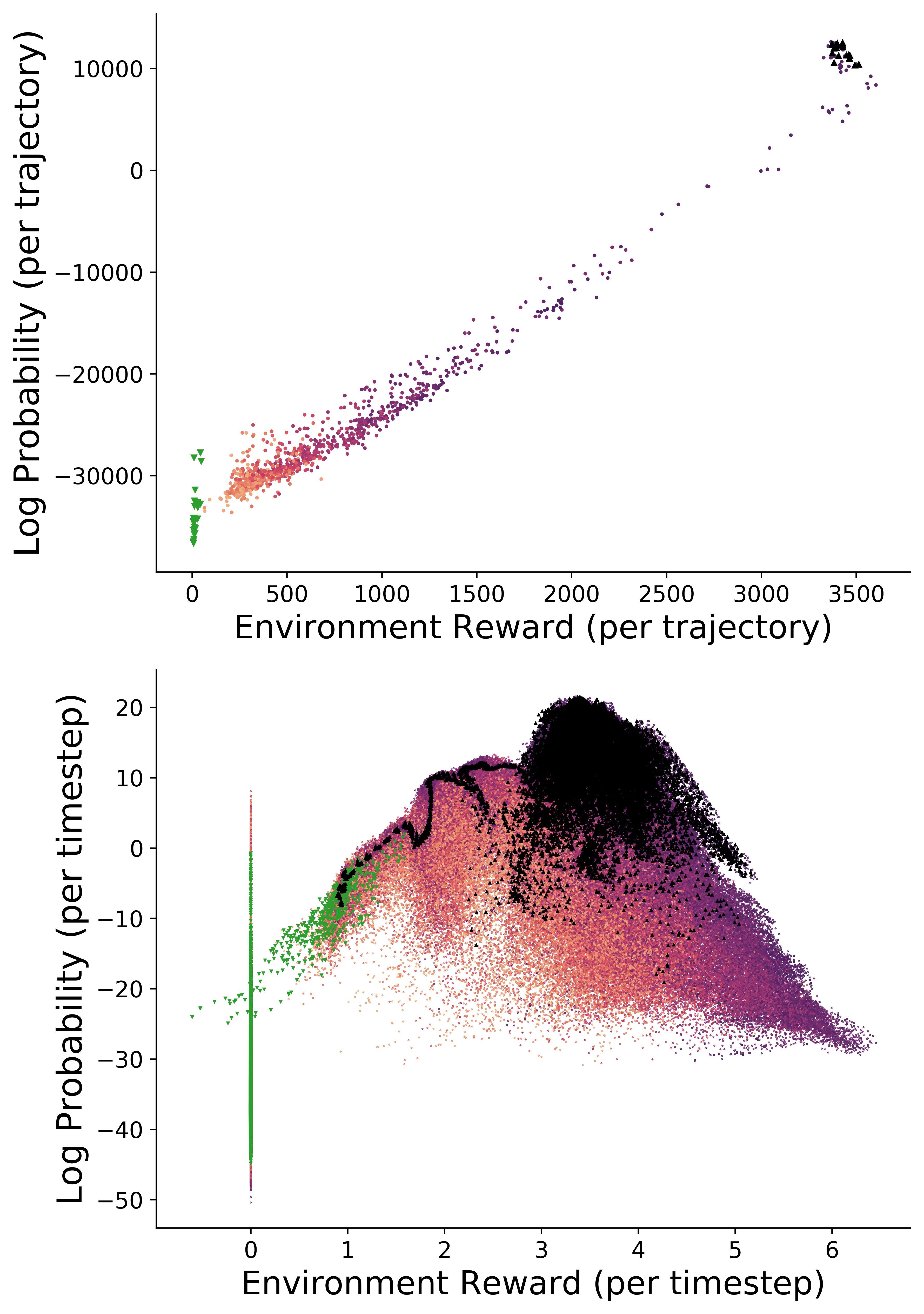
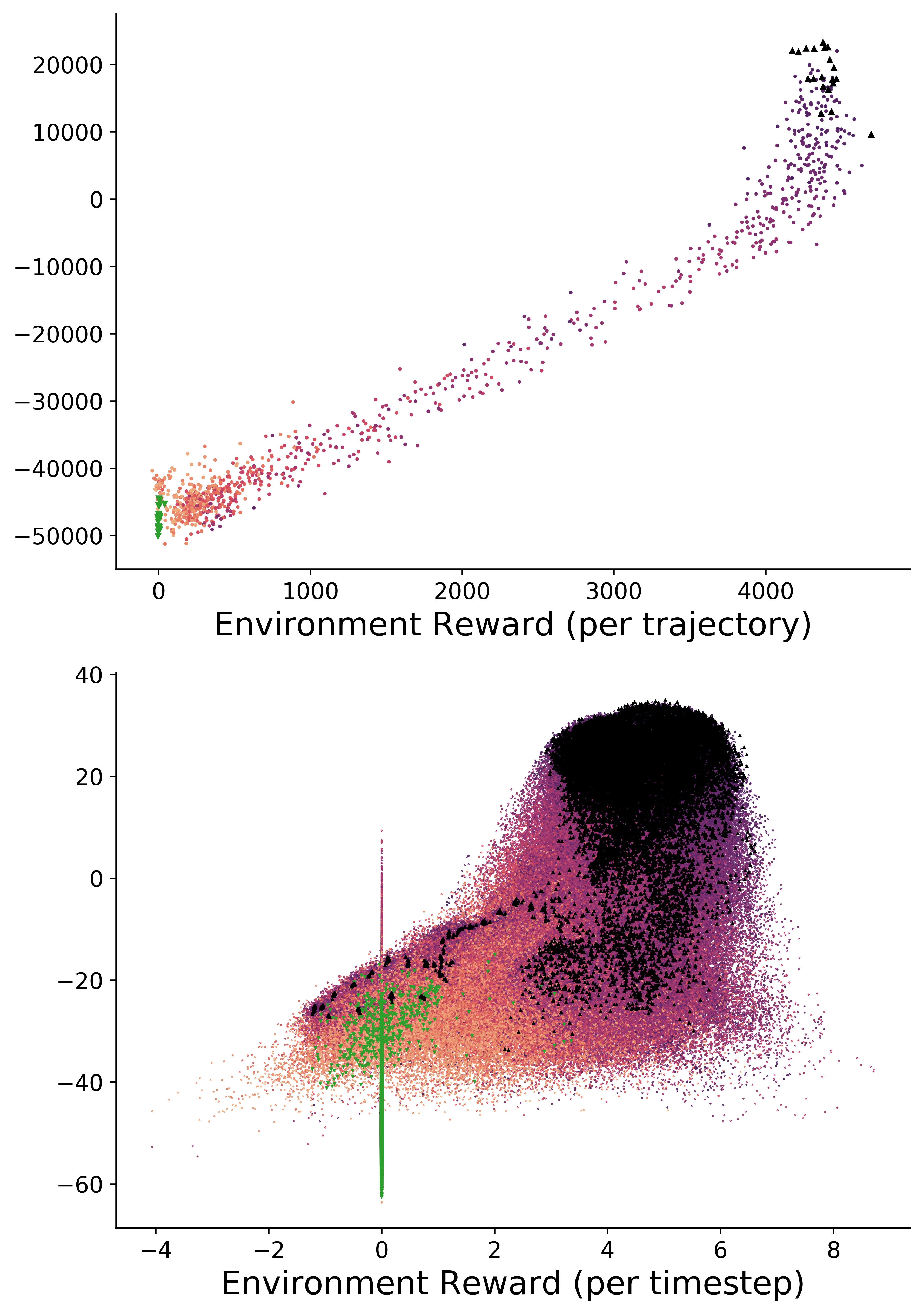
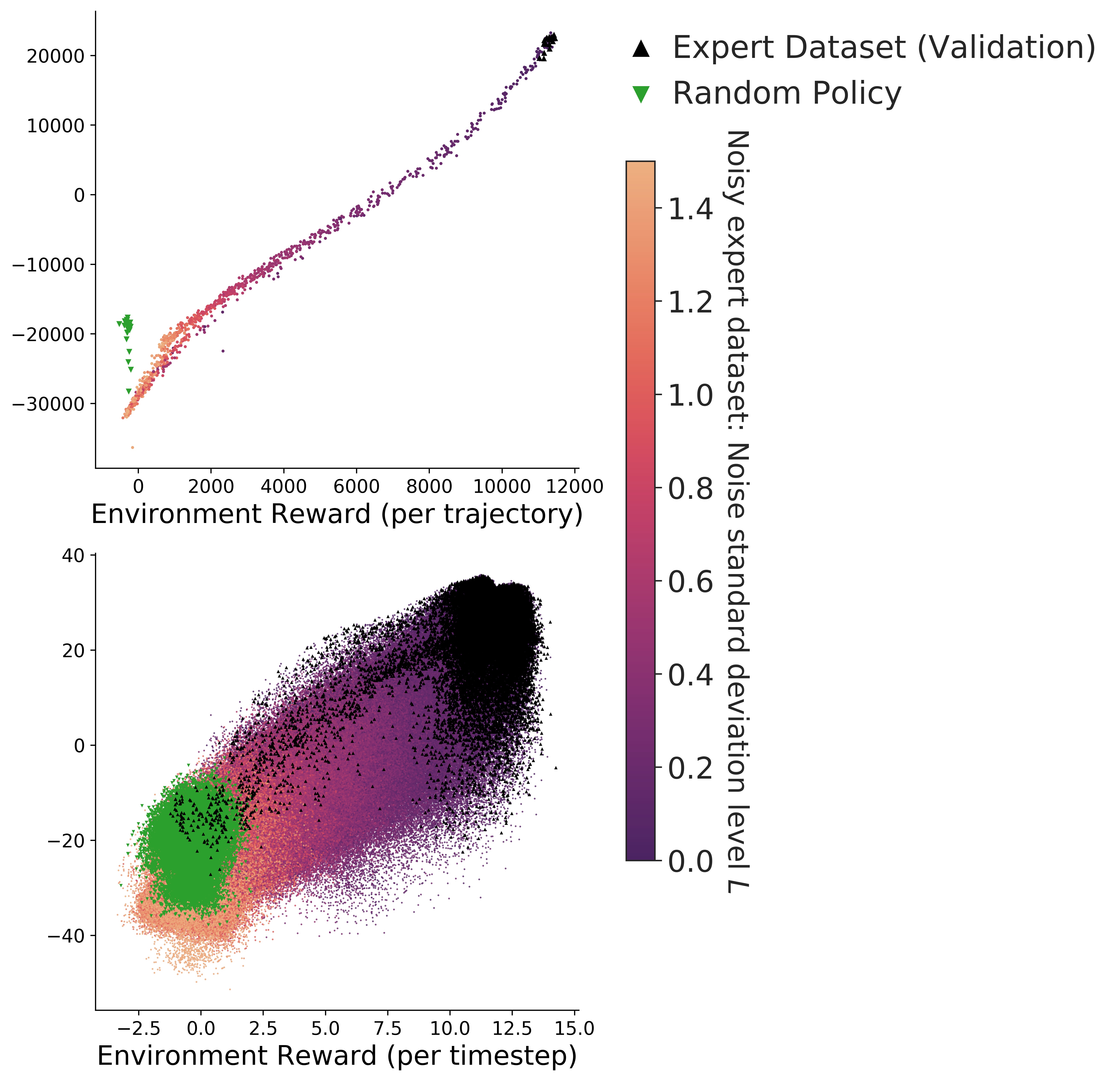
(a) Hopper	(b) Walker2d	(c) HalfCheetah

Figure 2: Log probability as a function of environment rewards for Hopper, Walker2d, and HalfCheetah. Trajectory-wise (top row) and step-wise (bottom row). The expert demonstration validation dataset (black) has highest log probability (and environment reward), while a randomly initialized policy (green) gets assigned a very low log probability. See description of the noisy expert dataset in Appendix IL-flOw: Imitation Learning from Observation using Normalizing Flows.

Appendix A Datasets Descriptions

For visualization purposes we also collect for each environment a "noisy expert" dataset, which we’ll refer to as $D_{Enoisy}$, consisting of 1000 trajectories from the expert policies with a fixed amount of additive Gaussian action noise sampled throughout each trajectory. Hence for a given trajectory in this dataset, we first sample a noise level $L\sim\mathcal{U}(0,1.5)$, and we add to the expert actions at each timestep noise $\omega\sim\mathcal{N}(0,L)$. We find that a standard deviation $L=1.5$ is enough to bring the expert policy to a random policy level of performance. This dataset allows us to inspect our learnt reward signal for trajectories in the environment generated by behaviors closer ($L\downarrow$) or further to the expert ($L\uparrow$) in policy space, the additive noise being on the actions. Further policies naturally translates to further state space explored in this noisy dataset as well. $D_{Enoisy}$ is shown in the ‘Flare’ yellow to purple colormap on Figure 2.

$D_{random}$ is the dataset containing transitions from the RL agent’s warmup/exploration phase, using a uniform random policy $\pi_{rdm}(a|s)\sim\mathcal{U}(A_{min},A_{max})$, with $A_{min},A_{max}$ the environment action bounds. $D_{random}$ is shown in green on Figure 2.

Appendix B Derivations for Eqns. 4 and 5

Eq. 4

$$\mathcal{H}(p_{\pi}) =-\mathbb{E}_{s_{0:T-1}\sim p_{\pi}(\tau)}\left[\sum_{t=0}^{T-1}\log p_{\pi}(s_{t+1}|s_{t})\right]$$ (7)

$$=\sum_{t=0}^{T-1}-\mathbb{E}_{s_{0:T-1}\sim p_{\pi}(\tau)}\left[\log p_{\pi}(s_{t+1}|s_{t})\right]$$ (8)

$$=\sum_{t=0}^{T-1}-\mathbb{E}_{s_{0:t+1}\sim p_{\pi}(\tau)}\left[\log p_{\pi}(s_{t+1}|s_{t})\right]$$ (9)

$$=\sum_{t=0}^{T-1}\mathbb{E}_{s_{0:t}\sim p_{\pi}(\tau)}\left[\mathcal{H}\left(p_{\pi}(\cdot|s_{t})\right)\right]$$ (10)

$$=\mathbb{E}_{s_{0:T}\sim p_{\pi}(\tau)}\left[\sum_{t=0}^{T-1}\mathcal{H}\left(p_{\pi}(\cdot|s_{t})\right)\right].$$ (11)

Eq. 5

$$\mathcal{H}\left(p_{\pi}(\cdot|s_{t})\right) =-\int p_{\pi}(s_{t+1}|s_{t})\log p_{\pi}(s_{t+1}|s_{t})\mathrm{d}s_{t+1}$$ (12)

$$=-\int\pi(a_{t}|s_{t})\log\left(\left|\frac{\mathrm{d}a_{t}}{\mathrm{d}s_{t+1}}\right|\pi(a_{t}|s_{t})\right)\mathrm{d}a_{t}$$ (13)

$$=-\int\pi(a_{t}|s_{t})\log\pi(a_{t}|s_{t})\mathrm{d}a_{t}-\int\pi(a_{t}|s_{t})\log\left|\frac{\mathrm{d}a_{t}}{\mathrm{d}s_{t+1}}\right|\mathrm{d}a_{t}$$ (14)

$$=\mathcal{H}\left(\pi(\cdot|s_{t})\right)+\mathbb{E}_{a_{t}\sim\pi}\left[\log\left|\frac{\mathrm{d}s_{t+1}}{\mathrm{d}a_{t}}\right|\right]$$ (15)

If the dynamics are approximately linear in the support of $\pi(a_{t}|s_{t})$, then the second term becomes a constant and may be ignored for policy optimization.

Appendix C Extra Experiments

C.1 Noise Regularized Normalizing Flow

We need to ensure this density model is representative of the expert demonstration state distributions. By using the generative capabilities of normalizing flows, which are the inverse operation of their density estimation mode, we can inspect the effect of the noise regularization process, as well as fit of our density model.

Moreover, we should ensure that the expert dataset samples have the highest log likelihood , and that samples away from the expert trajectories are assigned sensible log likelihoods. We can probe the trained transition density function anywhere and examine the sample’s log probabilities.

Single step sampling

: For each dataset $D_{E},D_{Enoisy}$, given a sample $s$, we sample next state predictions $s^{\prime}_{expert}$ given conditioning variables $s$ and a noise level $h\leq h_{max}$. We can visualize the noise regularization process this way. See Figure 3.

Reward calibration plots

: For each dataset $D_{E},D_{Enoisy},D_{random}$ we compare the environment ground truth reward with the learnt reward function. See Figure 2.

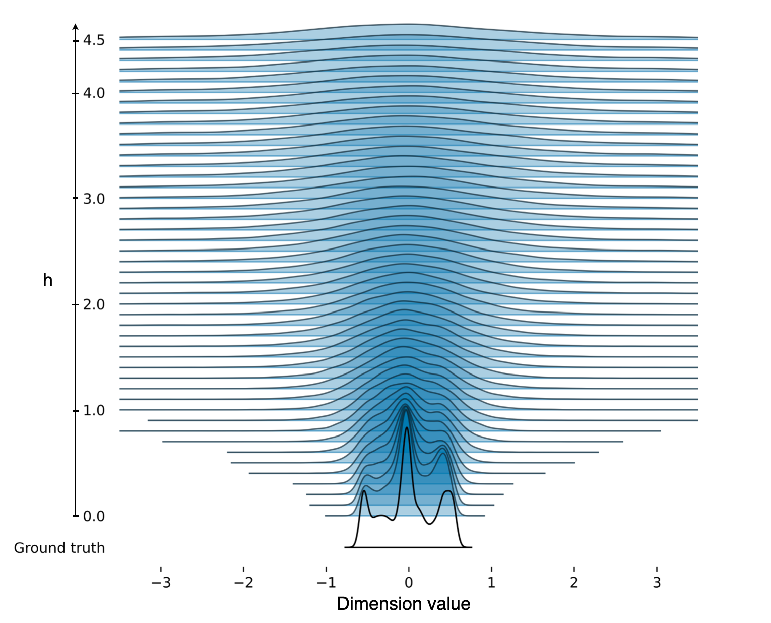
Figure 3: $p_{e}(s^{\prime}|s)$ density distributions for the 10th dimension of Hopper-v2, for the expert transition training dataset in black, and the normalizing flow model learnt noise conditional distribution in blue. Higher values of $h$ correspond to regularized versions of the training dataset distribution, smoothly extending its support.

Appendix D Hyperparameters

D.1 Soft Actor Critic

Parameter	Value
Entropy regularization coefficient $\alpha$	0.1
Automatic entropy tuning	False
$\tau$	5e-4
Actor network architecture (hidden)	[512, 512]
Critic network architecture (hidden)	[1024, 1024]
Actor LR	3e-4
Critic LR	3e-4
Optimizer	Adam
Actor non linearity	Tanh
Critic non linearity	ReLU

Table 2: SAC Hyperparameters

D.2 Neural Spline Flows

Parameter	Value
Training epochs	1000
LR	5e-4
Spline bins	8
Network size (hidden)	[8, 8]
Transform type	Rational quadratic coupling
Mask type	Alternating binary
Number of flow layers	3
Base distribution	Conditional Diagonal Normal
Optimizer	AdamW
Weight Decay	1e-4
$h_{min}$	0.0
$h_{max}$	4.5
Non linearity	Sine($\omega_{0}=2\pi)$
Spectral Normalization	True

Table 3: Neural Spline Flow Hyperparameters

References

- [1] Brian D Ziebart, Andrew L Maas, J Andrew Bagnell, and Anind K Dey. Maximum entropy inverse reinforcement learning. In AAAI, volume 8, pages 1433–1438, 2008.
- [2] Jonathan Ho and Stefano Ermon. Generative adversarial imitation learning. In Advances in Neural Information Processing Systems, pages 4565–4573, 2016.
- [3] Seyed Kamyar Seyed Ghasemipour, Richard Zemel, and Shixiang Gu. A divergence minimization perspective on imitation learning methods. In Conference on Robot Learning, pages 1259–1277. PMLR, 2020.
- [4] Tianwei Ni, Harshit Sikchi, Yufei Wang, Tejus Gupta, Lisa Lee, and Ben Eysenbach. f-irl: Inverse reinforcement learning via state marginal matching. In Conference on Robot Learning, 2020.
- [5] Kuno Kim, Akshat Jindal, Yang Song, Jiaming Song, Yanan Sui, and Stefano Ermon. Imitation with neural density models. CoRR, abs/2010.09808, 2020.
- [6] Robert Dadashi, Léonard Hussenot, Matthieu Geist, and Olivier Pietquin. Primal wasserstein imitation learning. arXiv preprint arXiv:2006.04678, 2020.
- [7] Tuomas Haarnoja, Aurick Zhou, Pieter Abbeel, and Sergey Levine. Soft actor-critic: Off-policy maximum entropy deep reinforcement learning with a stochastic actor. In International Conference on Machine Learning, volume 80, pages 1861–1870. PMLR, 2018.
- [8] Eric T. Nalisnick, Akihiro Matsukawa, Yee Whye Teh, Dilan Görür, and Balaji Lakshminarayanan. Do deep generative models know what they don’t know? In 7th International Conference on Learning Representations, ICLR 2019, New Orleans, LA, USA, May 6-9, 2019. OpenReview.net, 2019.
- [9] Polina Kirichenko, Pavel Izmailov, and Andrew G Wilson. Why normalizing flows fail to detect out-of-distribution data. In H. Larochelle, M. Ranzato, R. Hadsell, M. F. Balcan, and H. Lin, editors, Advances in Neural Information Processing Systems, volume 33, pages 20578–20589. Curran Associates, Inc., 2020.
- [10] Ian J. Goodfellow, Jean Pouget-Abadie, Mehdi Mirza, Bing Xu, David Warde-Farley, Sherjil Ozair, Aaron Courville, and Yoshua Bengio. Generative adversarial networks, 2014.
- [11] Martín Arjovsky and Léon Bottou. Towards principled methods for training generative adversarial networks. In 5th International Conference on Learning Representations, ICLR 2017, Toulon, France, April 24-26, 2017, Conference Track Proceedings. OpenReview.net, 2017.
- [12] Tim Salimans, Ian Goodfellow, Wojciech Zaremba, Vicki Cheung, Alec Radford, and Xi Chen. Improved techniques for training gans. Advances in neural information processing systems, 29:2234–2242, 2016.
- [13] Martin Arjovsky, Soumith Chintala, and Léon Bottou. Wasserstein generative adversarial networks. In International conference on machine learning, pages 214–223. PMLR, 2017.
- [14] Chin-Wei Huang, Faruk Ahmed, Kundan Kumar, Alexandre Lacoste, and Aaron Courville. Probability distillation: A caveat and alternatives. In Ryan P. Adams and Vibhav Gogate, editors, Proceedings of The 35th Uncertainty in Artificial Intelligence Conference, volume 115 of Proceedings of Machine Learning Research, pages 1212–1221. PMLR, 22–25 Jul 2020.
- [15] Jonas Rothfuss, Fabio Ferreira, Simon Boehm, Simon Walther, Maxim Ulrich, Tamim Asfour, and Andreas Krause. Noise regularization for conditional density estimation, 2020.
- [16] Hyeongju Kim, Hyeonseung Lee, Woo Hyun Kang, Joun Yeop Lee, and Nam Soo Kim. Softflow: Probabilistic framework for normalizing flow on manifolds. In H. Larochelle, M. Ranzato, R. Hadsell, M. F. Balcan, and H. Lin, editors, Advances in Neural Information Processing Systems, volume 33, pages 16388–16397. Curran Associates, Inc., 2020.
- [17] Conor Durkan, Artur Bekasov, Iain Murray, and George Papamakarios. Neural spline flows. In H. Wallach, H. Larochelle, A. Beygelzimer, F. d'Alché-Buc, E. Fox, and R. Garnett, editors, Advances in Neural Information Processing Systems, volume 32. Curran Associates, Inc., 2019.
- [18] Emanuel Todorov, Tom Erez, and Yuval Tassa. Mujoco: A physics engine for model-based control. In IEEE/RSJ International Conference on Intelligent Robots and Systems (IROS), pages 5026–5033. IEEE, 2012.