Constraint-Based Causal Structure Learning from Undersampled Graphs

Abstract

Graphical structures estimated by causal learning algorithms from time series data can provide highly misleading causal information if the causal timescale of the generating process fails to match the measurement timescale of the data. Existing algorithms provide limited resources to respond to this challenge, and so researchers must either use models that they know are likely misleading, or else forego causal learning entirely. Existing methods face up-to-four distinct shortfalls, as they might a) require that the difference between causal and measurement timescales is known; b) only handle very small number of random variables when the timescale difference is unknown; c) only apply to pairs of variables (albeit with fewer assumptions about prior knowledge); or d) be unable to find a solution given statistical noise in the data. This paper aims to address these challenges. We present an algorithm that combines constraint programming with both theoretical insights into the problem structure and prior information about admissible causal interactions to achieve speed up of multiple orders of magnitude. The resulting system scales to significantly larger sets of random variables ($>100$) without knowledge of the timescale difference while maintaining theoretical guarantees. This method is also robust to edge misidentification and can use parametric connection strengths, while optionally finding the optimal among many possible solutions.

1 Introduction

Dynamic causal models play a pivotal role in modeling real-world systems in diverse domains, including economics, education, climatology, and neuroscience. Given a sufficiently accurate causal graph over random variables, one can predict, explain, and potentially control some system; more generally, one can understand it. In practice, however, specifying or learning an accurate causal model of a dynamical system can be challenging for both statistical and theoretical reasons.

One particular challenge arises when data are not measured at the speed of the underlying causal connections. For example, fMRI scanning of the brain measures bloodflow and oxygen level changes in different brain regions, thereby indirectly measuring neural activity (which leads to increased oxygen consumption). fMRI thus provides data about an important dynamical system, but these measures take place (at most) every second while the brain’s actual dynamics is known to proceed at a faster rate Oram and Perrett (1992), though we do not know how much faster. In general, when the measurement timescale is significantly slower than the causal timescale (as with fMRI), learning can output importantly incorrect causal information. For instance, if we only measure every other timestep in Figure 1, then the true graph (top left) would differ from the data graph (top right). For example, we might conclude that variable $2$ directly influences variable $5$, when variable $3$ is the actual direct cause. This type of error can lead to inefficient or costly methods of control. More generally, understanding of a system depends on the causal-timescale (i.e., non-undersampled) causal relations, not the measurement-timescale (apparent) relations.

In this paper, we consider the problem of learning the causal structure at the causal timescale from data collected at an unknown measurement timescale. This challenge has received significant attention in recent years Plis et al. (2015b); Gong et al. (2015); Hyttinen et al. (2017); Plis et al. (2015a), but all current algorithms have significant limitations (see Section 2) that make them unusable for many real-world scientific challenges. Current algorithms show the theoretical possibility of causal learning from undersampled data, but their practical applicability is limited to small graph sizes, sometimes including only a pair of variables Gong et al. (2015). In contrast, we present a provably correct and complete algorithm that can operate on 100-node graphs and hence be potentially useful in biological and other domains for learning causal timescale structure from undersampled data.

2 Related Work And Notation

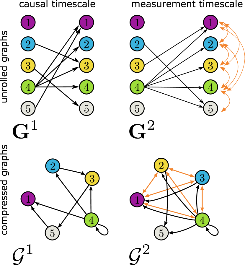
Figure 1: Causal graph $\mathbf{G}^{1}$ and its undersampled version $\mathbf{G}^{2}$: unrolled and compressed versions.

A directed dynamic causal model is a generalization of “regular” causal models Pearl et al. (2000); Spirtes et al. (1993): graph G includes $n$ distinct nodes for random variables $\textbf{V}=\{V_{1},V_{2},...,V_{n}\}$ at both the current timestep $t$ (V^t), and also each previous timesteps (V^t-k) in which there is a direct cause of some $V_{i}^{t}$. We assume that the “true” underlying causal structure is first-order Markov: the independence $\textbf{V${}^{t}$}\perp\!\!\!\perp\textbf{V${}^{t-k}$}\mid\textbf{V${}^{t-1}$}$ holds for all $k>1$ (i.e. causal sufficiency assumption Spirtes et al. (2000)). G is thus over $2\textbf{V}$, and the only permissible edges are $V^{t-1}_{i}\rightarrow V^{t}_{j}$, where possibly $i=j$. The quantitative component of the dynamic causal model is fully specified by parameters for $P(\textbf{V}^{t}|\textbf{V}^{t-1})$. We assume that these conditional probabilities are stationary over time, but the marginal $P(\textbf{V}^{t})$ need not be stationary.

We denote the timepoints of the underlying causal structure as $\{t^{0},t^{1},t^{2},...,t^{k},...\}$. The data are said to be undersampled at rate $u$ if measurements occur at $\{t^{0},t^{u},t^{2u},...,t^{ku},...\}$. We denote undersample rate with superscripts: the true causal graph (i.e., undersampled at rate $1$) is G¹ and that same graph undersampled at rate $u$ is G^u. To determine the implied G at other timescales, the graph is first “unrolled” by adding instantiations of G¹ at previous and future timesteps, where V^t-2 bear the same causal relationships to V^t-1 that V^t-1 bear to V^t, and so forth. In this unrolled (time-indexed by $t$) graph, all V at intermediate timesteps are not measured; this lack of measurement is equivalent to marginalizing out (the variables in) those timesteps to yield G^u. This problem has been parametrically addressed by Gong et al. (2015). Yet, a very interesting approach proposed in the paper was demonstrated only on a 2-variable system. Although an interesting approach, it has not been developed further and made practical.

Various representations have been developed for graphs with latent confounders, including partially-observed ancestral graphs (PAGs) Richardson and Spirtes (2002) and maximal ancestral graphs (MAGs) Zhang (2008). However, these graph-types cannot easily capture the types of latents produced by undersampling Mooij and Claassen (2020). Instead, we use compressed graphs, along with properties that were previously proven for this representation Danks and Plis (2013). A condensed graph includes only V, where temporal information is implicitly encoded in the edges. In particular, a condensed graph version $\mathcal{G}$ of dynamic causal graph G has $V_{i}\rightarrow V_{j}$ in $\mathcal{G}$ iff $V^{t-1}_{i}\rightarrow V^{t}_{j}$ is in G. Undersampling (i.e., marginalizing intermediate timesteps) is a straightforward operation for compressed graphs: (1) $V_{i}\rightarrow V_{j}$ in $\mathcal{G}^{u}$ iff there is a length-$u$ directed path from $V_{i}$ to $V_{j}$ in $\mathcal{G}^{1}$ iff there is a directed path from $V^{t-u}_{i}$ to $V^{t}_{j}$ in G¹; and (2) $V_{i}\leftrightarrow V_{j}$ in $\mathcal{G}^{u}$ iff there exists length-$s<u$ directed paths from $V_{k}$ to $V_{i}$, and to $V_{j}$, in $\mathcal{G}^{1}$ (i.e., $V_{k}$ is an unobserved common cause in G¹ fewer than $u$ timesteps back). See Appendix for additional proofs. The bottom row of Figure 1 shows compressed graphs for the unrolled ones on the top row; the left shows the causal timescale and the right shows the graphs undersampled at rate $2$.

Figure 2: Comparison of sRASL (red) with previous state-of-the-art RASL (blue).

Given this framework, the overall causal learning challenge can now be restated as: given $\mathcal{G}^{u}$ but not $u$ (or given dataset D at unknown undersample rate), what is the set of possible $\mathcal{G}^{1}$? There will often be many possible $\mathcal{G}^{1}$ for given $\mathcal{G}^{u}$, and so we use $\llbracket\mathcal{H}\rrbracket$ to denote the equivalence class of $\mathcal{G}^{1}$ that could yield $\mathcal{H}$ (the given causal graph inferred from data D) for some $u$. That is, $\llbracket\mathcal{H}\rrbracket=\{\mathcal{G}^{1}:\exists u(\mathcal{G}^{u}=\mathcal{H})\}$ Various algorithms have been developed to infer $\llbracket\mathcal{H}\rrbracket$, each with distinctive shortcomings. There are $2^{n^{2}}$ possible $\mathcal{G}^{1}$, so perhaps unsurprisingly, this problem is NP-complete:

Theorem 1 (Hyttinen et al. (2017)[Theorem 1]).

Deciding whether a consistent G¹ exists for a given $\mathcal{H}$ is NP-complete, for all undersampling rates $u\geq 2$.

Mesochronal Structure Learning (MSL) Plis et al. (2015b) showed it is possible to learn $\llbracket\mathcal{H}\rrbracket$ in a non-brute force manner if we know $u$. Every edge in G^u corresponds to one or more paths of length $u$ in G¹, and so G¹ can be constructed by identifying $u-1$ intermediate nodes for each edge in G^u. MSL searches the state space of possible identifications in a Depth-First Search (DFS) manner. Each identification implies a G¹, and if G^u $=\mathcal{H}$, then $\textbf{G}^{1}\in\llbracket\mathcal{H}\rrbracket$. Otherwise, search continues. MSL backtracks in the DFS whenever some G^u includes an edge that is absent from $\mathcal{H}$, as the candidate G¹ and all its supergraphs cannot be in $\llbracket\mathcal{H}\rrbracket$.

Although Plis et al. (2015b) showed that the concept that causal inference from undersampled data is feasible, MSL is computationally intractable on even moderate-sized graphs. Hyttinen et al. (2017) used the implied constraints to develop an Answer Set Programming (ASP) Simons et al. (2002); Niemelä (1999); Gelfond and Lifschitz ; Lifschitz (1988) method that formulated this causal inference challenge as a rule-based constraint satisfaction problem. ASP is a rule-based declarative constraint satisfaction paradigm that is well-suited for representing and solving various NP-hard problems (e.g. Theorem 2). In essence, the algorithm in Hyttinen et al. (2017) takes as input the measured causal graph $\mathcal{H}$, determines the set of implied constraints on G¹, and then uses the general-purpose Answer Set Solver Clingo Gebser et al. (2011) to determine the set of possible $\textbf{G}^{1}$ significantly faster than MSL. The same idea of using Boolean satisfiability solvers to integrate (in)dependent data constraints has been used for various other causal learning challenges Hyttinen et al. (2013); Triantafillou et al. (2010).

Although the method in Hyttinen et al. (2017) is significantly faster, one must specify the undersampling rate $u$ (or else run the method sequentially for all possible $u$, thereby losing much of the computational advantage). In contrast, the Rate-Agnostic (Causal) Structure Learning (RASL) approach (with three different versions) Plis et al. (2015a) makes no such assumption. These algorithms are similar to MSL, but consider each possible $u$ for some $\textbf{G}^{1}$. RASL reduces computational complexity with two additional stopping rules for given $\textbf{G}^{1}$: (1) if some $\textbf{G}^{k}$ has previously been seen, then further undersampling of $\textbf{G}^{1}$ will not produce new graphs; and (2) if G^k is not an edge-subset of $\mathcal{H}$ for all $k$, then do not consider any edge-superset of G¹ Plis et al. (2015a). However, despite these improvements, RASL still faces memory and run-time constraints for even moderate numbers of nodes.

One key observation from all of these learning algorithms is the importance of strongly connected components (SCCs) Danks and Plis (2013):

Definition 2.1.

An SCC in compressed graph $\mathcal{H}$ is a maximal set of nodes $\mathcal{\textbf{S}}\subseteq\mathcal{\textbf{V}}$ such that, for every $X,Y\in\mathcal{\textbf{S}}$ there is a directed path from X to Y .

Note that the variables in a compressed graph $\mathcal{H}$ can be fully partitioned based on SCC membership. SCCs can be highly stable, as the node-membership of an SCC will not change as we undersample, as long as the greatest common divisor (gcd) of the set of lengths of all simple loops (directed cycles without repeated nodes) in the SCC is $1$:

Theorem 2 (Danks and Plis (2013)[Theorem 3]).

S is an SCC in $\textbf{G}^{u}$ for all $u$ iff gcd($\mathcal{L_{S}})$ = 1 for SCC $\mathcal{\textbf{S}}\in\textbf{G}^{1}$

In this paper, we develop sRASL (for solver-based RASL), a novel algorithm that leverages insights from multiple sources, such as the constraints implied by SCC stability (Theorem 2). We show that sRASL significantly outperforms previous methods. The contributions of this paper are threefold: first, we reformulated the RASL algorithm from a search-based procedure to a constraint satisfaction problem encoded in a declarative language Fahland et al. (2009). Second, this reformulation enables us to add additional constraints based on SCC structure, and thereby gain significant speed-up. Third, we ensure that sRASL provides a straightforward way to find approximate solutions when $\mathcal{H}$ is an unreachable graph (i.e., when $\llbracket\mathcal{H}\rrbracket=\emptyset$). These advances collectively provide up to three orders of magnitude improvements in speed, thereby enabling causal inference given undersampling data involving over $100$ nodes. As a concreate example of the improvements, Figure 2 compares sRASL (red) with the previously-fastest RASL Plis et al. (2015a) method (blue) on the same graphs. The same input graph $\mathcal{H}$ took RASL nearly $1000$ minutes to compute $\llbracket\mathcal{H}\rrbracket$, but only $6$ seconds for sRASL.

3 sRASL: Optimized ASP-based Causal Discovery

The sRASL algorithm takes as input a (potentially) undersampled graph $\mathcal{H}$, whether learned from data D, expert domain knowledge, a combination of the two, or some other source. sRASL’s agnosticism about the source of the input graph enables wider applicability, as we can use whatever information is available Danks and Plis (2019). In the asymptotic (data) limit, the sRASL output is the full $\llbracket\mathcal{H}\rrbracket$.

sRASL leverages the fact that connections between SCCs in $\mathcal{H}$ must form a directed acylic graph. More specifically: if $X\rightarrow Y$ with $X\in\textbf{A},Y\in\textbf{B}$ for SCCs $\textbf{A}\neq\textbf{B}$, then $C\not\leftarrow D$ for all $C\in\textbf{A},D\in\textbf{B}$. Moreover, Theorem 2 provides the (weak) condition under which SCC membership is preserved under undersampling. These two observations imply that structural features potentially provide additional constraints beyond the obvious ones (See Section4.3). In particular, if $\mathcal{H}$ has a roughly modular structure–that is, the SCCs are not too large–then sRASL generates many more constraints than the algorithm of Hyttinen et al. (2017).

Listing 1 shows the Clingo (for a brief Introduction on Clingo and Answer Set Programming, refer to Appendix C) code of sRASL, which is based on exactly representing the conditioning and marginalization operations (defined in Section 2) in ASP. In the first line, we input the first-order graph-specific specification of $\mathcal{H}$ (e.g., the edge $1\rightarrow 10$ translates to $\operatorname{hdirected}(1,10)$). Line $2$ encodes the second-order structure of $\mathcal{H}$, including the partition of V into SCCs. These predicates and basic descriptive information are added to the Clingo code (lines $3,4,5$) in an automated way.

maxu on line $3$ specifies the maximum undersampling rate, as there is provably such a $u$ where $\mathcal{G}^{u}=\mathcal{G}^{k}$ for all $k>u$, if we have the same condition that leads to stable SCC membership:

Theorem 3 (Plis et al. (2015a)[Theorem 3.1]).

If gcd($\mathcal{L_{S}})$ = 1 for all SCCs $\textbf{S}\subseteq\textbf{V}$, then $\mathcal{G}^{u}=\mathcal{G}^{u+1}$ for all $u>f\leq n_{F}+\gamma+d+1$.

where $\gamma$ is the transit number, $d$ is graph diameter and $n_{F}$ is the Frobenius number. In practice, the plausible undersampling rate will often be much lower than the theoretical upper bound in Theorem 3. For example, consider fMRI data. The underlying rate of brain activity is generally thought to be $\sim 100$ milliseconds and fMRI devices measure approximately every two seconds. Hence, $u=20$ is a plausible upper bound on undersampling in fMRI studies.

⬇

1%( * input graph edge specifications here * e.g.: hdirected(1,5) ... )

2%( * input graph SCC specifications here * e.g.: sccsize(0, 5). scc(1, 0) ...)

3#const n = 10, maxu = 20

4node(1..n).

51 {u(1..maxu)} 1.

6{edge1(X,Y)} :- node(X), node(Y).

7directed(X, Y, 1) :- edge1(X, Y).

8directed(X, Y, L) :- directed(X, Z, L-1),

9 edge1(Z, Y), L <= U, u(U).

10bidirected(X, Y, U) :- directed(Z, X, L), directed(Z, Y, L), node(X;Y;Z), X < Y, L < U, u(U).

11:- directed(X, Y, L), not hdirected(X, Y), node(X;Y), u(L).

12:- bidirected(X, Y, L), not hbidirected(X, Y), node(X;Y), u(L), X < Y.

13:- not directed(X, Y, L), hdirected(X, Y), node(X;Y), u(L).

14:- not bidirected(X, Y, L), hbidirected(X, Y), node(X;Y), u(L), X < Y.

15% the following is only used when SCC accounting is enabled

16:- edge1(X, Y), scc(X, K), scc(Y, L), K != L, sccsize(L, Z), Z > 1, not dag(K,L).

Listing 1: Clingo code for sRASL

⬇

1 :~ directed(X, Y, L), no_hdirected(X, Y, W), node(X;Y), u(L). [W@1,X,Y]

2 :~ bidirected(X, Y, L), no_hbidirected(X, Y, W), node(X;Y), u(L), X < Y. [W@1,X,Y]

3 :~ not directed(X, Y, L), hdirected(X, Y, W), node(X;Y), u(L). [W@1,X,Y]

4 :~ not bidirected(X, Y, L), hbidirected(X, Y, W), node(X;Y), u(L), X < Y. [W@1,X,Y]

Listing 2: Integrity constraints for turning sRASL algorithm into an optimization problem when they replace lines 11 through 14 in Listing 1

Line $6$ in Listing 1 stipulates that all edges in $\mathcal{G}^{1}$ are possible (by default), and so the output will contain any possible model that does not violate the integrity constraints of lines $11-16$. Lines $7$ and $8$ define paths of length $L$ in the graph (i.e., an edge in $\mathcal{G}^{L}$). As described in Section 2: $X\rightarrow Y\in\mathcal{G}^{u}\iff X\overset{u}{\rightsquigarrow}Y\in\mathcal{G}^{1}$ where $\overset{u}{\rightsquigarrow}$ is a path of length $u$. Line $10$ similarly defines bidirected edges in $\mathcal{G}^{L}$: $X\leftrightarrow Y\in\mathcal{G}^{u}\iff\exists Z,l:(X\overset{l}{\leftsquigarrow}Z\overset{l}{\rightsquigarrow}Y\in\mathcal{G}^{1})$.

Lines $11-14$ provide the core constraints, as they ensure that sRASL returns only $\mathcal{G}^{1}$ for which there exists $u$ such that $\mathcal{G}^{u}=\mathcal{H}$. Line $16$ adds the additional constraints based on impermissibility of cycles between SCCs. That is, if we consider each SCC as a super-node, Line $16$ ensures that the edges of the directed acyclic graph (DAG) connecting SCCs in $\mathcal{H}$ are not violated in the outputs.

If sRASL initially returns the empty set (i.e., there are no suitable $\mathcal{G}^{1}$), then it is possible to run sRASL in an optimization mode instead to find optimal (though not perfect) outputs (see Section 4.5 for details). One potential reason for $\llbracket\mathcal{H}\rrbracket=\emptyset$ is statistical noise or other errors in estimating or specifying $\mathcal{H}$. In such cases, sRASL finds the set of $\textbf{G}^{1}$ that are, for some $u$, closest to $\mathcal{H}$ by the objective function:

$$\mathcal{G}^{1*},u^{*}\in\operatorname*{\arg\!\min}\sum_{\begin{subarray}{c}e\in\mathcal{H}\end{subarray}}I[e\notin\mathcal{G}^{u}]\cdot w(e\in\mathcal{H})+\sum_{\begin{subarray}{c}e\notin\mathcal{H}\end{subarray}}I[e\in\mathcal{G}^{u}]\cdot w(e\notin\mathcal{H}),$$ (1)

where the indicator function $I(c)=1$ if the condition holds and zero otherwise. $w(e\in\mathcal{H})$ indicates the importance (i.e., reliability) of edge $e$; $w(e\notin\mathcal{H})$ indicates the reliability of the absence of an edge. Since $\mathcal{H}$ is an undersampled graph, it consists of directed and bidirected edges. We thus implement both $w(e\in\mathcal{H})$ and $w(e\notin\mathcal{H})$ as two pairs of $n\times n$ matrices, one pair for existence and absence of directed edges, and one pair for bidirected edges. To learn the optimal graph at the true causal timescale, for every $\mathcal{G}^{1}$ in the solutions set, the corresponding $\mathcal{G}^{u}$ is compared to the input $\mathcal{H}$ and penalized for the difference according to weights representing the reliability of the measurement timescale estimates.

In order to incorporate Equation 5 in Listing 1, we replace its exact integrity constraints (Lines 11-14) with the optimization formulation Gebser et al. (2011) in Listing 2. In Listing 2 we specify a weight for each edge (or lack there of) in $\mathcal{H}$ using W and the importance of these weights can be specified for each integrity constraint using the W@i syntax with i being the importance.

3.1 sRASL Completeness and Correctness

sRASL exhibits significant improvements in computation time, so it is important to show that we do not lose generality or theoretical guarantees. We demonstrate correctness and completeness using the notion of a direct encoding of the problem (i.e., the space of solutions is fully characterized, and any non-solution violates a constraint). We first prove (Appendix A) that we have provided a direct encoding:

Theorem 4.

Listing 1 is a direct encoding of the undersampling problem.

Clingo is a complete solver, based on CDNL (Conflict-Driven Nogood Learning) Drescher and Walsh (2011), itself based on CDCL (Conflict-Driven Clause Learning) Marques Silva and Sakallah (1996); Marques-Silva and Sakallah (1999). Hyttinen et al. (2014)[Theorem 2] and Hyttinen et al. (2013)[Section $5.2$] show that, if the ASP encoding is the direct encoding of the problem, then ASP will produce the complete set of solutions in the infinite sample space limit. In other words, Theorem 5 implies: since our algorithm yields at least one sound solution, Clingo will produce all possible solutions. Therefore, soundness results in completeness. That is, sRASL’s success is not due to heuristics or some incomplete or not-everywhere-correct algorithmic step.

4 Results

A major virtue of sRASL is its empirical performance, so we now consider a range of simulations (to ensure known ground truth) to understand this performance in more detail. For these experiments, we used Clingo in parallel mode using 10 threads and computing on AMD EPYC 7551 CPUs. To cope with the multiple repeated calculations and hundreds of graphs we have tested per parameter setting all experiments were run on a slurm cluster which submits jobs to one of the 19 machines on the same network. Each of the 19 nodes was equipped with 64 cores and 512 GB of RAM.

4.1 Comparing sRASL vs. RASL

We first compare sRASL with the existing RASL method (Figure 2). We generated $100$ 6-node SCCs for each density in $[0.2,0.25,0.3]$, and then undersampled each graph by $2,3$, and $4$. We used 6-node graphs as RASL struggles to handle larger graphs in reasonable time and space Plis et al. (2015a). Each column of Figure 2 consists of graphs of approximately same density (increasing density from left-to-right), and subcolumns represent different undersample rates (for that density). As Figure 2 shows, sRASL is typically three orders of magnitude faster than RASL, even on relatively small graphs.

4.2 Comparing Graph Size

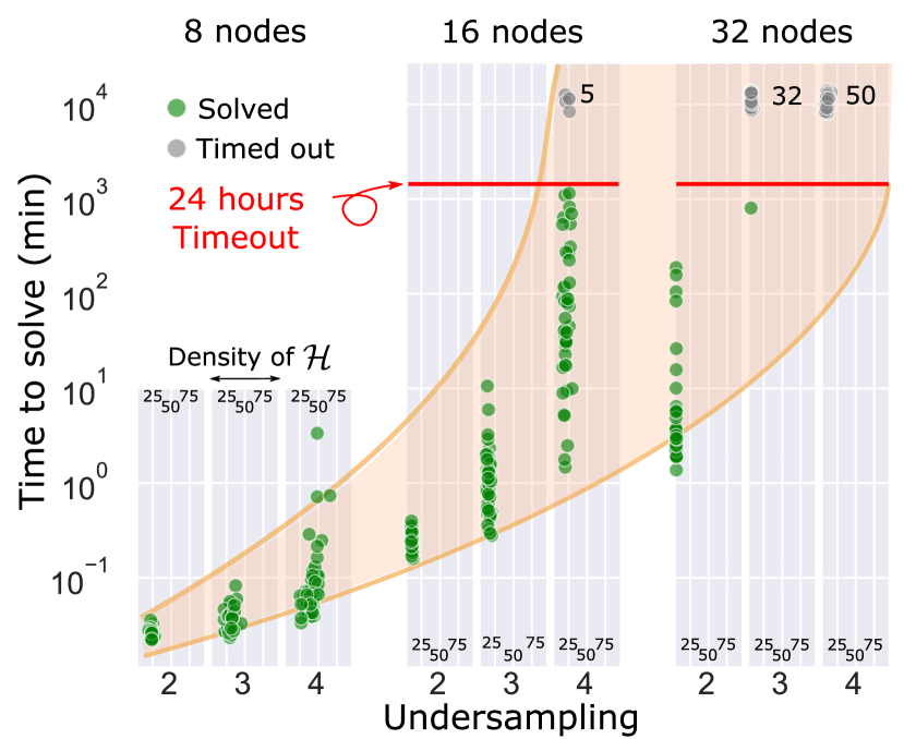
Figure 3: Time behavior of graphs of size $8,16$ and $32$. The time out for this experiment indicated by the red line was $24$ hours. Green dots represent graphs that has been computed within the 24-hours window. Gray represent graphs that could not be fully computed within $24-$hours window.

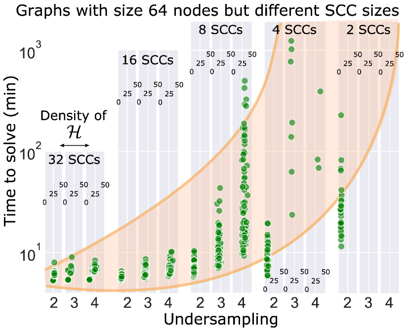
Figure 4: Time behavior of graphs of size $64$ with various sub SCC sizes. The time out for this experiment was $24$ hours ($1440$ Minutes).

It is perhaps unsurprising that sRASL runs much faster than RASL, as sRASL uses an ASP solver (which were previously known to yield faster algorithms Hyttinen et al. (2017)). We next wanted to see just how much larger the graphs could be. More generally, we aimed to better understand how sRASL’s computational performance scales with the number of nodes for single-SCC graphs. The focus on single SCCs is motivated by the theoretical need to understand the size-speed tradeoff, and also scientific applicability since many real-world systems consist of tightly coupled factors with many feedback loops (i.e., they are a single SCC). We consider multiple-SCC graphs in later subsections.

We generated $50$ random single-SCC graphs each of $8,16$ and $32$ nodes, all with average degree of $1.4$ outgoing edges per node. We then undersampled each graph by $2,3$ and $4$, and used each individual undersampled graph as input to sRASL. We used a 24-hour timeout (i.e., we stopped an sRASL run if it did not finish in 24 hours). Figure 4 shows the increasing computational costs as both number of nodes and undersample rate increase. Notably, sRASL was able to learn $\llbracket\mathcal{H}\rrbracket$ for $32$-node single-SCC graphs, though it reached timeout for all $\mathcal{H}$ at $u=4$ $32$-node graphs. That is, for low $u$, sRASL scales to much larger single-SCC graphs than RASL.

4.3 Comparing SCC Size

The other major innovation of sRASL is incorporation of constraints derived from the SCC structure. We thus investigated the performance of sRASL on large, structured, multiple-SCC graphs. Many real-world systems exhibit some degree of modularity, where there are dense or feedback connections within a module or subsystem, and relatively sparser connections between modules or subsystems. In theory, sRASL should perform well on these kinds of structures since it incorporates SCC-based constraints. Please refer to Appendix B for an ablation study on effect of using additional constraints for SCC structures.

We tested the value of SCC-based constraints using graphs with $64$ nodes that differed in their SCC structure. Specifically, we randomly generated $50$ graphs each of: $32$ size-$2$ SCCs; $16$ size-$4$ SCCs; $8$ size-$8$ SCCs; $4$ size-$16$ SCCs; or $2$ size-$32$ SCCs. We then undersampled each graph by $u=2,3$, or $4$, and ran sRASL (again with a 24-hour timeout).

Figure 4 shows the computation time for these graphs, with increasing SCC size (and decreasing number of SCCs) from left to right. The first key observation is that sRASL successfully found $\llbracket\mathcal{H}\rrbracket$ for $64$-node graphs, at least when there was some internal structure. Second, and relatedly, we observe a wide range of computation times for these graphs, even though all had the same number of nodes ($64$). We clearly see the impact of SCC structure, as sRASL was dramatically faster when there were many small SCCs, rather than a few large SCCs. The results in Figure 4 might seem to suggest an “upper bound” around $30$ nodes for sRASL. But the results in Figure 4 make it clear that any potential “upper bound” is primarily on the number of nodes in the SCCs, rather than the total number of nodes in the graph.

4.4 Comparing Graph Size With Constant SCC Size

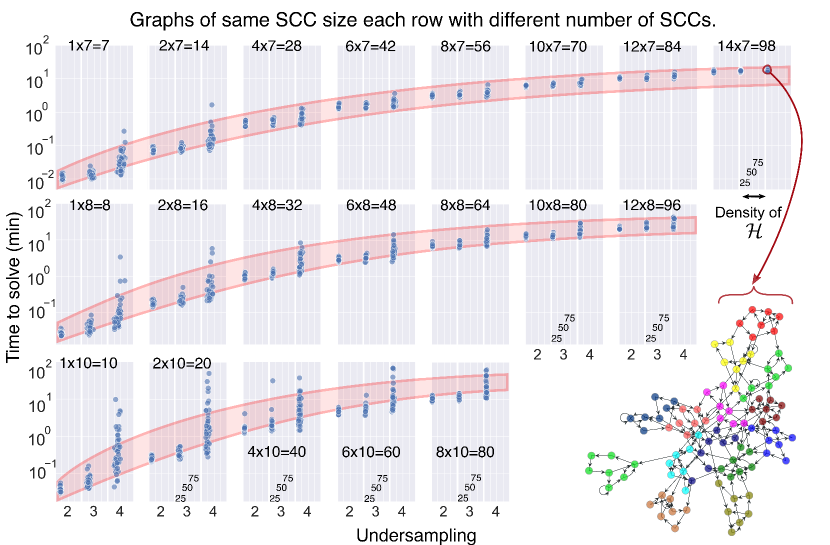
Figure 5: Time behaviour of graphs with the same SCCs sizes but with multiple number of SCCs. Top row graphs of SCC size $7$ with $1,2,...,14$ number of SCCs. Middle row graphs of SCC size $8$. Bottom row graphs of SCC size $10$.Bottom right corner is an example of a structured graph with $98$ nodes structured as $14$ SCCs of size $7$. Each color represents one Strongly Connected Component.

The previous results suggest that sRASL might be able to solve much larger graphs, as long as the SCCs are not overly large. More generally, the previous simulations showed that sRASL’s computational cost scales (at least) exponentially in the size of the SCC, but did not reveal how it scales in the number of SCCs.

We again generated $50$ different graphs for each of several settings. We considered SCCs with $7$, $8$, and $10$ nodes, and varied the number of SCCs within the graph (again for $u=2,3$, and $4$). Figure 5 shows the computational cost of sRASL, where each row includes graphs with SCCs of the same size, but the number of SCCs increasing from left-to-right. The critical observation here is that the time complexity grows approximately linearly, rather than exponentially (or worse). For example, the graph shown in Figure 5 has $98$ nodes, but sRASL successfully computes $\llbracket\mathcal{H}\rrbracket$ in approximately $20$ minutes. (Recall that RASL took $17$ hours to compute a graph with only $6$ nodes.)

This simulation demonstrates that sRASL is usable on relatively large graphs, as long as there is appropriate internal structure. One might worry, though, whether real-world systems do not have the right structure. If we consider fMRI (brain) data, Sanchez-Romero et al. (2019) recently aggregated a number of simulations of realistic causal graphs for brain processes studied with fMRI, and the largest SCC in these widely-accepted models has only seven nodes. Moreover, typical brain parcellations contain $50-100$ regions (= nodes), and sRASL can easily handle graphs with $100$ nodes if the SCC size is in the $8-10$ range.

The results in this subsection suggest that we could potentially find $\llbracket\mathcal{H}\rrbracket$ for each larger graphs, as long as they were composed of reasonably-sized SCCs. However, we found that the Clingo language and solver seems to be limited in the number of atoms that it can handle. In our simulations, graphs of size $100$ seem to be the limit for Clingo to handle all the predicates. An open question is whether sRASL can be optimized to produce fewer predicates (or Clingo improved to handle more atoms).

4.5 Optimization

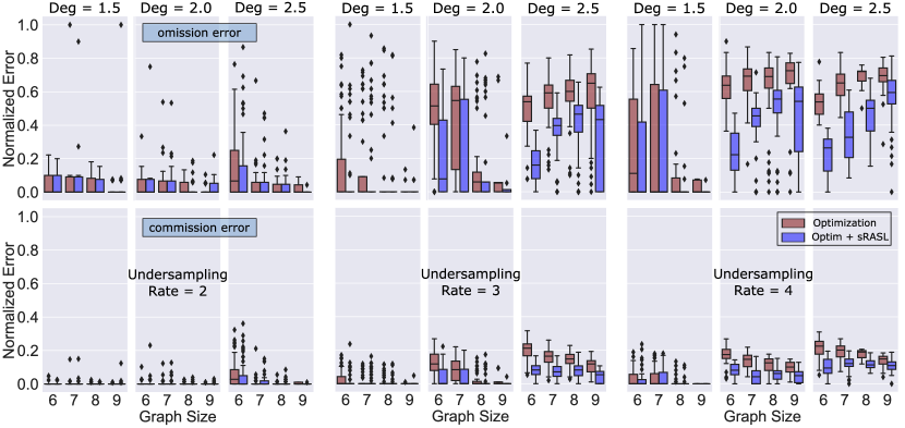
Figure 6: The omission (top) and commission (bottom) error of different graph sizes and undersampling of two, three and four from left to right.

Finally, we explored the optimization capability of Clingo. Recall that sometimes $\llbracket\mathcal{H}\rrbracket=\emptyset$ due to statistical errors or other noise in learning $\mathcal{H}$. Clingo can solve an optimization problem based on user-specified weights and priorities, and output a single solution with minimum cost function (along with $u$ for this solution). In particular, we can use Clingo to find $\mathcal{G}^{1}$ whose $\mathcal{G}^{u}$ (for some $u$) are closest (relative to the edge weights) to $\mathcal{H}$.

In this simulation, we first randomly generate $\mathcal{G}^{1}$ and undersample it to a random $u$ to get $\mathcal{G}^{u}=\mathcal{H}$ such that $\llbracket\mathcal{H}\rrbracket\neq\emptyset$. We then assign weights to the edges of $\mathcal{H}$ and randomly break one edge from it. We then run sRASL on this “broken” $\mathcal{H}$ to learn a suitable $\mathcal{G}^{1}$. Red bars in Figure 6 show the edge omission and commission errors for this approach. We see that, except for high undersamplings, the optimization capability of Clingo can be used to frequently retrieve the true $\mathcal{G}^{1}$; that is, this version of sRASL is robust to small errors in $\mathcal{H}$ in many settings.

A more complex approach to finding suitable solutions is to first run the optimization method to identify a solution G${}^{1}_{opt}$ and undersample rate $u_{opt}$. We can then undersample this solution G${}^{1}_{opt}$ by $u_{opt}$ to get G${}^{u}_{opt}$. We then use sRASL to obtain $\llbracket\textbf{G}^{u}_{opt}\rrbracket$ (i.e., the full equivalence class of the undersampled graph that is “nearest” to $\mathcal{H}$). We then compute the error based on the minimum error among all $\textbf{G}^{1}\in\llbracket\textbf{G}^{u}_{opt}\rrbracket$; that is, we ask whether the true graph was actually found. This approach is motivated by the intended use of sRASL by domain scientists, where the final decision on which graph in the equivalence class better suits the question is made by the scientist using the algorithm. Blue bars in Figure 6 show that this more complex method provides improved performance compared to regular optimization.

5 Conclusion and Discussion

Real-world scientific problems frequently involve measurement processes that operate at a different timescale than the causal structure of the system under study. As causal learning and analysis methods are increasingly used to address societal and policy challenges, it is increasingly critical that we use methods that reveal usable information (while also being clear when we cannot infer some information). Obviously, like any method, sRASL could yield information that is misused, but the aim here is to provide another useful tool in the scientists’ policy-makers’ toolboxes. If measurements occur at a slower rate than the causal influences, then causal discovery from those undersampled data can yield highly misleading outputs. Multiple methods have been developed to infer aspects of the underlying causal structure from the undersampled data/graph. However, the assumptions or computational complexities of those algorithms make them unusable for most real-world challenges. In this paper, we have developed and tested sRASL, a novel algorithm that is less subject to those same limitations. More specifically, sRASL provides all consistent solutions (without knowledge of exact undersampling rate) for large ($100$-node) graphs in a usable amount of time. sRASL also shows reasonable robustness to statistical error in the estimated graph by finding the closest consistent solution. Future research will focus on application of sRASL to actual neuroimaging data, and extensions to situations with multiple measurement modalities.

6 Acknowledgement

This work was supported by NIH R01MH129047 and in part by NSF 2112455, and NIH 2R01EB006841

Appendix A Appendix

We start with proving some results used in conversion of the DBN structures to their compressed graph representations.

Lemma 1.

For all $u$, $G_{u}$ contains no directed edges between variables at the same time step.

Proof.

$u=1$ holds by assumption for $G_{1}$. For $u>1$, every directed edge corresponds to a directed path of length $u$ in $G_{1}$. Since all directed edges in $G_{1}$ are from $t-1$ to $t$ (or more generally, from $t-k$ to $t-(k+1)$), every directed path in $G_{1}$ is from an earlier time step to the current one. Hence, no directed edge in $G_{u}$ can be from $V_{i}^{t}$ to $V_{j}^{t}$. ∎

Lemma 2.

If the Markov order of $G_{1}$ is $1$, then the Markov order of all $G_{u}$ is also $1$ (relative to measurement at rate $u$).

Proof.

The Markov order of a dynamic causal graph is the smallest $m$ such that $\textbf{V}^{t}$ is independent of $\textbf{V}^{t-r}$ given $\textbf{V}^{t-1},\ldots,\textbf{V}^{t-m}$ for all $r>m$. If the Markov order of $G_{1}$ is $1$, then all paths from $\textbf{V}^{t-r}$ to $\textbf{V}^{t}$ must be blocked by $\textbf{V}^{t-1}$ for $r>1$. Since graphical structure is replicated across timesteps, it follows that all paths from $\textbf{V}^{t-r}$ to $\textbf{V}^{t}$ must be blocked by $\textbf{V}^{t-u}$ for $r>u$. Therefore, the Markov order of $G_{u}$ is $u$, which corresponds to Markov order $1$ for measurements at rate $u$. ∎

The following theorem demonstrates correctness of our ASP algorithm.

Theorem 5.

Listing 1 is a direct encoding of the undersampling problem.

Proof.

We will prove this by contradiction. Let us call the undersampled input graph to the algorithm $\mathcal{H}$, considering that is the undersampled version of a graph G${}^{1}_{true}$ at rate $u_{true}$. By definition, every directed edge in $\mathcal{H}$ corresponds to a path of length $u_{true}$ in G${}^{1}_{true}$. Similarly, every bidirected edge in $\mathcal{H}$ corresponds to an unobserved common cause fewer than $u_{true}$ timesteps back(refer to Section 2 for exact definition). Line $7-11$ in Listing 1 considers all such G¹s without exclusion. Let us call the set all the pairs of graphs and corresponding undersampling rates $u$ described by Listing 1 S.

Let us assume there is a pair G${}^{1}_{a}$ and $u_{a}$ that is in S but if we undersample G${}^{1}_{a}$ by $u_{a}$, let us call it G${}^{u}_{a}$, will not be the same as $\mathcal{H}$. If G${}^{u}_{a}$ has an extra directed(bidirected) edge, this will contradict with line 12(13) of Listing 1. Similarly, if $\mathcal{H}$ has a directed(bidirected) edge that in not present in G${}^{u}_{a}$, it will contradict with line 14(16). Therefore, Listing 1 is a direct encoding of the undersampling problem. ∎

Appendix B The Effects of Accounting for SCCs In sRASL

In this section, we show the results of additional experiments on the effects of accounting for strongly connected components (SCCs) when the graph has a modular structure (i.e., consists of several interconnected strongly connected components). For this experiment, we generated 50 random graphs sized $8$ to $15$ with multiple SCCs as described in Table1. Then on the same set of graphs, we ran sRASL once with using our additional constraints for SCC structures and once without accounting for the modular structure. We limited the computational resources available to each run to $24$ hours time cutoff with a RAM limit of $50$ GB. The results presented in Figure8 show that using additional constraints to account for SCC structure dramatically reduces the time and memory needed to compute equivalent classes for undersampled graphs. Furthermore, the difference between time and memory requirements to solve for these graphs with and without constraints for SCCs increases for larger graphs as the computational requirements for the latter grow at a much faster pace. This result allows us to handle much larger graphs as shown in Figure 5 of the main paper.

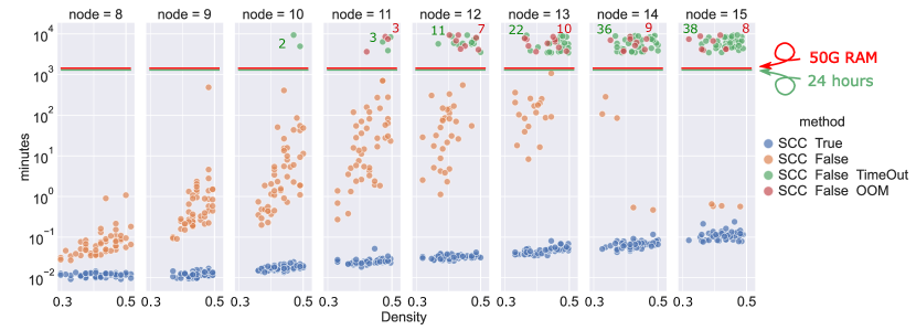
Figure 7: Time behavior of the same set of graphs when solved with and without accounting for additional constraints accounting for the SCC structure. While sRASL most of the $15$-node graphs in a $24$ hours period without the SCC constraints due to either timeout or Out Of Memory error(OOM), the longest it takes to solve a $15$-node graph with SCC constraints is $14$ seconds. None of the graphs failed to compute the complete equivalence class within the time and memory allocated when solved accounting for the SCC structure.

Table 1: Number of SCCs and nodes per SCC of the graphs in the benchmark dataset

Num Nodes	8	9	10	11	12	13	14	15
Num SCCs	2	3	3	3	3	3	3	3
SCC Sizes	4,4	3,3,3	3,3,4	3,4,4	4,4,4	4,4,5	4,5,5	5,5,5

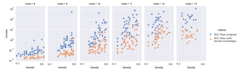
Figure 8: A knowledge of a definite presence of an edge in ${\cal G}^{1}$ between, for example, nodes 3 and 4, i.e. $V^{t}_{3}\rightarrow V^{t+1}_{4}$, can be easily encoded by adding ‘ edge1(3,4).‘ to Listing 1. In this experiment, we have added knowledge about a pair of arbitrary selected edges of ${\cal G}^{1}$ to the problem specification (orange dots) and compared the run time with the ASP specification that does not include this additional information about the solution (blue dots). The time out for the new computation was set to 1 hours and the examples were all the same as the ones already shown in Figure 1. The speed up with the additional constraints is clearly visible on the plots.

Appendix C Brief Introduction on clingo and Answer Set Programming (ASP)

clingo Gebser et al. [2011] combines a grounder gringo and a solver clasp. clingo is a declarative programming system based on logic programs and their answer sets, used to accelerate solutions of computationally involved combinatorial problems. The grounder converts all parts of a clingo program to “atoms,” (grounds the statements) and the solver finds “stable models.” In ASP, the answer set is a model in which all the atoms are derived from the program and each “answer” is a stable model where all the atoms are simultaneously true.

A general clingo program includes three main sections, which we show below using our algorithm as an example:

1. Facts: these are the known elements of the problem. For example, the input to Listing 1 is a graph for which we know the edges. A directed edge from node 1 to node 5 is in $\mathcal{H}$ translates to hdirected(1,5) (line 1) or if node 1 is part of the SCC number 2, we state this fact in clingo by scc(1,2) (line 2).

2. Rules: much like an if-else statement, a rule in clingo consists of a body and a head, formatted as head :- body. If all the literals in the body are true, then the head must also be true. Rules can include variables (starting with capital letters), and they are used to derive new facts after grounding. For example:

   directed(X, Y, 1) :- edge1(X, Y). (2)

   means that for any instantiations of the variables $X$ and $Y$, if we have an edge from $X$ to $Y$, there is a directed path from $X$ to $Y$ of length 1. Before this line, if the model contained the fact edge1(2,3), this line would generate a new fact: directed(2,3,1).

   Another type of rule is the “choice rule” that describes all the possible ways to choose which atoms are included in the model. For example, in line $5$ of Listing 1 we used a choice rule to state that the undersampling rate u can be anything from 1 to maxu. The cardinality constraint:

   {u(1..20)}. (3)

   will generate $2^{20}$ different models (they will not all actually be generated if they conflict with other predicate in each model, or else it would not be possible). In each of these $2^{20}$ models, one subset of all possible atoms generated with this choice rule exists ($\phi$, {u(1)}, {u(1), u(2)}, …). An example of an unconstrained choice rule is line 6 in Listing 1, where we want to generate one model for each possible way edges can be present in a graph between two nodes $X$ and $Y$. We can also limit the choice rule. In our problem, only one undersampling rate is present at each solution. We limit the cardinality constraint to have only one member in each model:

   1 {u(1..20)} 1. (4)

   the $1$ on the left is the minimum instantiations of this atom in the model and the $1$ on the right is the maximum. Therefore, we only generate $\binom{20}{1}=20$ models with this rule, namely one for each undersampling rate. Having several choice rules will multiply the number of generated models by each choice rule.

3. Integrity Constraints: if choice rules are to generate new models, integrity constraints are there to remove the wrong models from the answers set. More specifically, an integrity constraint is of the form:

   :- L0, L1, … . (5)

   where literals ${L_{0},L_{1},....}$ cannot be simultaneously positive. For example, in line $16$ of Listing1, we have:

   :- edge1(X, Y), scc(X, K), scc(Y, L), K != L, (6)

   sccsize(L, Z), Z > 1, not dag(K,L).

   for cases where the graph consists of several SCCs that are connected using a DAG. If the SCCs are connected by a cyclic directed graph, then the whole graph will become one big Strongly Connected Component. Integrity constraint 6 states that if there is not a directed edge from a node in SCC K to a node in SCC L as part of the initial DAG, there cannot be such edge1(X, Y) from node X to node Y, if node X is in SCC K and node Y is in SCC L.

References

- Danks and Plis [2013] David Danks and Sergey Plis. Learning causal structure from undersampled time series. In NIPS Workshop on Causality, volume 1, pages 1–10, 2013.
- Danks and Plis [2019] David Danks and Sergey Plis. Amalgamating evidence of dynamics. Synthese, 196(8):3213–3230, 2019.
- Drescher and Walsh [2011] Christian Drescher and Toby Walsh. Conflict-driven constraint answer set solving with lazy nogood generation. In Twenty-Fifth AAAI Conference on Artificial Intelligence, 2011.
- Fahland et al. [2009] Dirk Fahland, Daniel Lübke, Jan Mendling, Hajo Reijers, Barbara Weber, Matthias Weidlich, and Stefan Zugal. Declarative versus imperative process modeling languages: The issue of understandability. In Enterprise, Business-Process and Information Systems Modeling, pages 353–366. Springer, 2009.
- Gebser et al. [2011] Martin Gebser, Benjamin Kaufmann, Roland Kaminski, Max Ostrowski, Torsten Schaub, and Marius Schneider. Potassco: The Potsdam answer set solving collection. Ai Communications, 24(2):107–124, 2011.
- [6] M Gelfond and V Lifschitz. The stable model semantics for logic programming. ICSLP, 1988.
- Gong et al. [2015] Mingming Gong, Kun Zhang, Bernhard Schoelkopf, Dacheng Tao, and Philipp Geiger. Discovering temporal causal relations from subsampled data. In International Conference on Machine Learning, pages 1898–1906. PMLR, 2015.
- Hyttinen et al. [2013] Antti Hyttinen, Patrik O Hoyer, Frederick Eberhardt, and Matti Jarvisalo. Discovering cyclic causal models with latent variables: A general SAT-based procedure. arXiv preprint arXiv:1309.6836, 2013.
- Hyttinen et al. [2014] Antti Hyttinen, Frederick Eberhardt, and Matti Järvisalo. Constraint-based Causal Discovery: Conflict Resolution with Answer Set Programming. In UAI, pages 340–349, 2014.
- Hyttinen et al. [2017] Antti Hyttinen, Sergey Plis, Matti Järvisalo, Frederick Eberhardt, and David Danks. A constraint optimization approach to causal discovery from subsampled time series data. International Journal of Approximate Reasoning, 90:208–225, 2017.
- Lifschitz [1988] V Lifschitz. The stable model semantics for logic programming, 1988.
- Marques-Silva and Sakallah [1999] Joao P Marques-Silva and Karem A Sakallah. GRASP: A search algorithm for propositional satisfiability. IEEE Transactions on Computers, 48(5):506–521, 1999.
- Marques Silva and Sakallah [1996] J.P. Marques Silva and K.A. Sakallah. GRASP-A new search algorithm for satisfiability. In Proceedings of International Conference on Computer Aided Design, pages 220–227, 1996. doi: 10.1109/ICCAD.1996.569607.
- Mooij and Claassen [2020] Joris M Mooij and Tom Claassen. Constraint-based causal discovery using partial ancestral graphs in the presence of cycles. In Conference on Uncertainty in Artificial Intelligence, pages 1159–1168. PMLR, 2020.
- Niemelä [1999] Ilkka Niemelä. Logic programs with stable model semantics as a constraint programming paradigm. Annals of mathematics and Artificial Intelligence, 25(3):241–273, 1999.
- Oram and Perrett [1992] MW Oram and DI Perrett. Time course of neural responses discriminating different views of the face and head. Journal of neurophysiology, 68(1):70–84, 1992.
- Pearl et al. [2000] Judea Pearl et al. Models, reasoning and inference. Cambridge, UK: CambridgeUniversityPress, 19:2, 2000.
- Plis et al. [2015a] Sergey Plis, David Danks, Cynthia Freeman, and Vince Calhoun. Rate-agnostic (causal) structure learning. In Advances in neural information processing systems, pages 3303–3311, 2015a.
- Plis et al. [2015b] Sergey Plis, David Danks, and Jianyu Yang. Mesochronal structure learning. In Uncertainty in artificial intelligence: proceedings of the… conference. Conference on Uncertainty in Artificial Intelligence, volume 31. NIH Public Access, 2015b.
- Richardson and Spirtes [2002] Thomas Richardson and Peter Spirtes. Ancestral graph Markov models. The Annals of Statistics, 30(4):962–1030, 2002.
- Sanchez-Romero et al. [2019] Ruben Sanchez-Romero, Joseph D Ramsey, Kun Zhang, Madelyn RK Glymour, Biwei Huang, and Clark Glymour. Estimating feedforward and feedback effective connections from fMRI time series: Assessments of statistical methods. Network Neuroscience, 3(2):274–306, 2019.
- Simons et al. [2002] Patrik Simons, Ilkka Niemelä, and Timo Soininen. Extending and implementing the stable model semantics. Artificial Intelligence, 138(1-2):181–234, 2002.
- Spirtes et al. [1993] Peter Spirtes, Clark Glymour, and Richard Scheines. Causation, Prediction, and Search. Springer New York, 1993. doi: 10.1007/978-1-4612-2748-9. URL https://doi.org/10.1007/978-1-4612-2748-9.
- Spirtes et al. [2000] Peter Spirtes, Clark N Glymour, Richard Scheines, and David Heckerman. Causation, Prediction, and Search. MIT press, 2000.
- Triantafillou et al. [2010] Sofia Triantafillou, Ioannis Tsamardinos, and Ioannis Tollis. Learning causal structure from overlapping variable sets. In Proceedings of the Thirteenth International Conference on Artificial Intelligence and Statistics, pages 860–867. JMLR Workshop and Conference Proceedings, 2010.
- Zhang [2008] Jiji Zhang. Causal reasoning with ancestral graphs. Journal of Machine Learning Research, 9:1437–1474, 2008.