Scalable Multi-view Clustering with Graph Filtering

Abstract

With the explosive growth of multi-source data, multi-view clustering has attracted great attention in recent years. Most existing multi-view methods operate in raw feature space and heavily depend on the quality of original feature representation. Moreover, they are often designed for feature data and ignore the rich topology structure information. Accordingly, in this paper, we propose a generic framework to cluster both attribute and graph data with heterogeneous features. It is capable of exploring the interplay between feature and structure. Specifically, we first adopt graph filtering technique to eliminate high-frequency noise to achieve a clustering-friendly smooth representation. To handle the scalability challenge, we develop a novel sampling strategy to improve the quality of anchors. Extensive experiments on attribute and graph benchmarks demonstrate the superiority of our approach with respect to state-of-the-art approaches.

1 Introduction

With the rapid advances in information technology, many data are collected from various views or appear in multiple modalities, which form the so-called multi-view data. In other words, the same object can be described from different angles with heterogeneous features kang2021structured . For instance, an image can be represented by different types of features, such as Gabor, HOG, GIST, and LBP; a text news can be translated into multiple languages. Each individual view contains some specific property that should be explored chao2021survey ; hou2018safe . Nowadays, many data are also described in graph or network, which is a popular data structure to characterize interdependent systems yu2021learning . For example, an academic network can represent the relations among authors. In reality, multiple types of relations exist, e.g., co-author and co-paper relations in academic network. Hence, multilayer graph or multiplex network (i.e., multiview graph) are often applied to describe such systems and each layer accounts for one type of relation. In practice, nodes in the graph are often attached with attributes and this kind of data are named attributed graph. Therefore, it is desirable to take full advantage of available information for better performance in the downstream tasks.

To analyze those kinds of multiview data, clustering is a widely used technique to unveil meaningful patterns of samples or nodes by dividing them into disjoint groups huang2021robust ; zhu2019PR . To address above heterogeneous challenge, many researchers have been dedicating efforts in developing methods that are able to effectively discover a common cluster pattern shared by various views mi2022multi ; liu2021refined . A straightforward way is to concatenate all multiple views features and apply conventional single-view clustering methods upon it. This naive approach, however, completely ignore the correlation among multiple views chen2020multi . Therefore, more complex methods are proposed, which are supposed to explore the consensus and complementary information across multiple views. For instance, kumar2011cotraining proposes a co-regularization technique to minimize the disagreement between each pair of views. Inspired by co-training strategy, kumar2011co finds the clusterings that agree across the views. Roughly speaking, the existing methods can be divided into two categories. The first class of methods try to fuse the features wang2020parallel ; liu2021incomplete , while the others integrate clusterings kang2020partition . Nevertheless, these methods are susceptible to poor quality data, which lead to degraded clustering performance.

Instead of operating on the raw features, some recent approaches manage to learning in latent space. For example, zhang2017latent assumes that multiple views are originated from one underlying latent representation and reconstructs multi-view data to obtain a common subspace representation, upon with subspace clustering technique is implemented. Motivated by the success of deep neural networks, some deep multi-view clustering techniques are also developed. For instance, li2019deep utilizes deep autoencoder to learn latent representations shared by multiple views and employs adversarial training to disentangle the latent space. To deal with graph data, fan2020one2multi leverages a graph autoencoder to learn node embeddings of one selected view and reconstruct multiple graphs. Hence, its performance heavily depends on the chosen view and it fails to make full use of available data. By contrast, cheng2020multi uses multiple graph autoencoders to extract multiple embeddings and find a common clustering. Although these methods have attractive performance, they have high computational complexity. Thus, the clustering of multi-view graph data is still at a nascent stage.

From above analysis, we can observe that the clustering methods for feature and graph data are developed individually and there is no general framework that is suitable for both types of data. Therefore, they cannot exploit the rich feature and topology information in attributed graph. Moreover, they perform poor on noisy data and have high complexity. To this end, in this paper, we propose a novel and generic clustering method for various multi-view data: Scalable Multi-view Clustering with graph filtering (SMC). Compared to existing works, it has two distinct properties. First, it achieves a clustering-friendly representation for each view. According to clustering assumption, the feature values of sample points belonging to the same class are similar. This can be realized by graph filtering technique developed in signal processing community, which renders the signal smooth. Second, to reduce the computation complexity, a novel sampling strategy is introduced based on the importance of nodes. Comprehensive experiments and analysis demonstrate the superiority of our method.

2 Related Work

2.1 Notations

Without loss of generality, we define multi-view data $\mathcal{G}=(\mathcal{V},\xi_{1},\cdots,\xi_{v},X^{1},\cdots,X^{v})$, where $\mathcal{V}$ denotes the set of $n$ nodes, $\xi_{v}$ is the edge set, $X^{v}=\{\emph{{x}}_{1}^{v},\cdots,\emph{{x}}_{n}^{v}\}^{\top}\in\mathbb{R}^{n\times d_{v}}$ is the $v$-th feature matrix of nodes. $\xi^{v}$ can be combined into the topology structure of graph $A^{v}$, and $a_{ij}^{v}$ reflects the relationship between node $i$ and node $j$. If a dataset don’t have a graph associated with it, we can build one for each view as discussed later. Then, $D^{v}=\emph{diag}(d_{1},\cdots,d_{n})\in\mathbb{R}^{n\times{n}}$ denotes the degree matrix of $A^{v}$, where $d_{i}=\sum_{j=1}^{n}a_{ij}^{v}$. The symmetrically normalized Laplacian can be derived as $L^{v}=I-(D^{v})^{-\frac{1}{2}}(A^{v})(D^{v})^{-\frac{1}{2}}$.

2.2 Multi-view Clustering

Among various multi-view clustering methods, graph-based approaches often produce more impressive performance. AMGL Nie2016Parameter is a multi-view spectral clustering model with an auto-weighting mechanism. MLRSSC Brbi2017Multi learns a joint subspace representation across all views with low-rank and sparsity constraints. RMSC xia2014robust pursues a latent low-rank transition probability matrix and obtains clustering results by standard Markov chain method. PwMC and SwMC nie2017self learn a shared graph from input graphs by applying a novel self-weighting strategy. MSC_IAS wang2019multi applies Hilbert–Schmidt Independence Criterion (HSIC) to maximize the learned similarity with its corresponding intact space. LMVSC kang2019large is proposed to tackle the scalability challenge of multi-view subspace clustering. Specifically, it learns a smaller similarity matrix by the idea of anchor. Based on it, SMVSC chen2021smoothed is further proposed to enjoy a smooth data representation. To process multi-view graph, PMNE liu2017principled is developed to learn embeddings. MNE zhang2018scalable is a scalable multi-view network embedding method. Nevertheless, these methods are designed for either feature or graph data and are not applicable to attributed graph data.

Latter, O2MAC fan2020one2multi is developed to cluster multi-view attributed graph. Similarly, HAN HAN presents a graph neural network for heterogeneous graph by combining with attention mechanism. However, they often fail to fully exploit the rich semantic information of multi-view data. Recently, MvAGC lin2021graph is proposed for multi-view attributed graph clustering and shows impressive performance with a shallow approach. It is flexible to explore high-order relations among nodes lin2021multi . In this paper, we aim to bring a generic framework for both feature and graph data.

3 Methodology

3.1 Graph Filtering

Given a feature matrix $X=[\emph{{x}}_{1},\cdots,\emph{{x}}_{n}]^{\top}\in\mathbb{R}^{n\times d}$ with $n$ samples and $d$ features, it can be treated as $d$ $n$-dimensional graph signals. A natural signal should be smooth on nearby nodes in term of the underlying graph, i.e., nearby nodes have close feature values dong2019learning . From another perspective, a smooth signal will contain more low-frequency basis signals than high-frequency ones. In general, high-frequency components are regarded as noise. Hence, a smooth signal is supposed to be free of noise and thus benefits downstream analysis. To recover a clean signal $\bar{X}$, we can solve the following problem:

$$\min_{\bar{X}}\|\bar{X}-X\|_{F}^{2}+\mu Tr(\bar{X}^{\top}L\bar{X}),$$ (1)

where $\mu\textgreater 0$ is a balance parameter. The first term is a fidelity term and the second term is graph Laplacian regularization, which means that $\bar{x}_{i}$ and $\bar{x}_{j}$ should be close if samples $i$ and $j$ are similar in original space. Taking the first-order derivative of the objective function w.r.t. $\bar{X}$ and setting it to zero, we have

$$\bar{X}=(I+\mu L)^{-1}X.$$ (2)

Above solution involves matrix inversion whose time complexity is $O(n^{3})$. Therefore, we approximate $\bar{X}$ by its first-order Taylor series expansion, namely, $\bar{X}=(I-\mu L)X$. More generally, filtering with $k$ times can be written as:

$$\bar{X}=(I-\mu L)^{k}X.$$ (3)

When $\mu=1/2$, it goes back to the previously used filter $\bar{X}=(I-L/2)^{k}X$. Therefore, Eq.(3) is a generalization of previous filter lin2021graph . Because it has a tunable parameter $\mu$, it gives us more flexibility on real datasets pan2021multi . For multi-view data, we could obtain a smooth representation for each view, i.e., $\bar{X^{i}}=(I-\mu{L^{i}})^{k}{X^{i}}$. $k$-order graph filtering captures the long-distance structure information of graph by aggregating features of neighbors up to $k$th-order, which makes adjacent nodes have similar feature values. In other words, graph filtering encodes the structure information into feature. Therefore, it provides an elegant way to integrate the rich feature and structure information.

3.2 Clustering

It is known that representation is crucial to the performance of machine learning algorithms. For clustering task, it is assumed that similar samples are more likely assigned into the same group. Therefore, it is reasonable to smooth the data before feeding them into clustering model. It has been shown that graph filtering indeed increases the distance between clusters, which in turn facilitates subsequent clustering ma2020towards . Therefore, $\bar{X}$ can be applied in various clustering methods. In this paper, we choose subspace clustering due to its intriguing performance lv2021pseudo . Following kang2019large ; chen2021smoothed , we utilize the self-expressiveness property of data, i.e., each sample can be expressed as a linear combination of other samples, to learn a similarity matrix, which characterizes the similarities between any two instances zhang2020twin . As for multi-view data $\bar{X^{i}}$, we obtain the similarity matrix for each view. The problem can be modeled as:

$$\min_{\{Z^{i}\}_{i=1}^{v}}\sum_{i=1}^{v}\|{\bar{X^{i}}}^{\top}-{{B^{i}}}(Z^{i})^{\top}\|_{F}^{2}+\alpha\|Z^{i}\|_{F}^{2},$$ (4)

where $\alpha$ is a trade-off parameter and $B^{i}=[b_{1}^{i},\cdots,b_{m}^{i}]\in{R^{d_{i}\times{m}}}$ is the anchor matrix for $i$-th view. Note that we replace $\bar{X^{i}}$ with ${B^{i}}$ in the first term to reduce the computation complexity. Previously, it constructs a $n\times n$ similarity matrix and applies spectral clustering to achieve clustering result, whose time complexity is up to $\mathcal{O}(n^{3})$. In Eq. (4), we just learn a smaller $n\times m$ similarity matrix $Z^{i}$ to alleviate the computation burden. Specifically, we select $m$ representative points for each view, which are supposed to reconstruct the corresponding $\bar{X}^{i}$ based on $Z^{i}$ that characterizes the similarities between $n$ original nodes and $m$ anchors. More details about anchor selection strategy are provided in section 3.4. Eq. (4) admits a closed-form solution.

Next, we concatenate $Z^{i}$ as $\bar{Z}=[Z^{1},\cdots,Z^{i},\cdots,Z^{v}]\in\mathcal{R}^{n\times mv}$. It has been shown that the spectral embedding matrix $Q\in\mathcal{R}^{n\times g}$, which consists of $g$ eigenvectors associated with the largest $g$ eigenvalues of $\sum_{i}{Z^{i}Z^{i^{\top}}}/v$, can be achieved by applying singular value decomposition (SVD) on $\bar{Z}$ kang2019large . Finally, K-means is implemented on $Q$ to obtain the final $g$ partitions.

3.3 Anchor Selection

It is easy to see from (4) that the choice of anchors will impact the solution. The mainstream approach adopts K-means or random sampling, which makes sense for general feature data. In particular, we run K-means on $\bar{X^{i}}$ and let $g$ cluster centers form $B^{i}$. However, this approach could be suboptimal for graph data since each node has different importance and K-means treats all nodes equally. It is natural to sample anchors based on the importance of nodes. Let’s define $q:\mathcal{V}\rightarrow{R^{+}}$ as the importance measure function and assign the probability to node $i$ that it will be chosen as the first member of anchor set $\mathcal{M}$:

$$p_{i}=\frac{q(i)^{\gamma}}{\sum_{j\in{\mathcal{V}}}(q(j)^{\gamma})},$$ (5)

where $\gamma\in R^{+}$, which makes the distribution sharp (for $\gamma\textgreater 1$) or smooth (for $\gamma\textless 1$). After that, we select $m-1$ distinct nodes without replacement. Specifically, each left node $i\in{\mathcal{V}\setminus{\mathcal{M}}}$ is chosen with a probability $p_{i}/{\sum_{j\notin{\mathcal{M}}}}p_{j}$ as the second anchor, and so on until $\lvert\mathcal{M}\rvert=m$. For simplicity, the total degree of each node, i.e., $q(i)=\sum_{k=1}^{v}\sum_{j\in{\mathcal{V}}}A^{k}_{ij}$, is employed to characterize its importance.

Algorithm 1 SMC

Input: multi-view feature $\{X^{i}\}_{i\in[1,v]}$, or multi-view graph $\{A^{i}\}_{i\in[1,v]}$ with feature $\{X^{i}\}_{i\in[1,v]}$
Parameter: filter order $k$, filter parameter $\mu$, trade-off parameter $\alpha$, anchor number $m$,
cluster number $g$, sampling parameter $\gamma$
Output: $g$ partitions

1:if only multi-view feature is available then

2:     Build a graph for each view based on certain graph construction method

3:     Apply $k$ times graph filter on $\{X^{i}\}_{i\in[1,v]}$ to obtain the representation $\bar{X}^{1},\cdots,\bar{X}^{i},\cdots,\bar{X}^{v}$

4:     Sample $m$ anchors by applying K-means on $\bar{X}^{i}$ to construct $B^{i}$.

5:else

6:     Apply $k$ times graph filter on $\{X^{i}\}_{i\in[1,v]}$ to obtain the representation $\bar{X}^{1},\cdots,\bar{X}^{i},\cdots,\bar{X}^{v}$

7:     Sample $m$ anchors with indexes ind and then choose $m$ rows from $\bar{X}^{i}$ to build $B^{i}$.

8:end if

9:Calculate ${Z^{i}}\in\mathbb{R}^{n\times m}$ in Eq. (4), which is composed of ${\bar{Z}}\in\mathcal{R}^{n\times mv}$

10:Compute $Q$ by performing SVD on ${\bar{Z}}$

11:Apply K-means to Q

3.4 Time Complexity

The overall procedures for our proposed method is outlined in Algorithm 1. Suppose $N$ is the number of nonzero elements of adjacency matrix $A$, the time complexity of performing graph filtering is $\mathcal{O}(Ndkv)$, where $d=\sum_{i}d_{i}$. Sampling anchors process takes $\mathcal{O}(mv)$ and solving $Z^{i}$ takes $\mathcal{O}(nm^{3}v)$. In addition, the computation of $Q$ costs $\mathcal{O}(m^{3}v^{3}+2mvn)$ and the subsequent K-means consumes $\mathcal{O}(ng^{2})$. In real applications, $A$ is often sparse, thus $N\ll n^{2}$. Furthermore, $m,v\ll n$. Thus, the overall complexity could be linear to the sample number $n$. It is worth mentioning that our algorithm is iteration-free and makes it appealing in practice. The implementation of our method is public available at: https://github.com/EricliuLiang/SMC.

4 Experiment

4.1 Datasets

We perform extensive experiments on several benchmark datasets to demonstrate the effectiveness of our model. We choose widely used multi-view datasets, including Handwritten, Caltech-7, Caltech-20, and Citeseer. Handwritten and Caltech are image datasets of digits and objects respectively. They both have six different views. Citeseer is a citation network whose nodes denote publications with two views. To apply graph filtering, we employ probabilistic neighbor method nie2016constrained to obtain a graph for these datasets. Furthermore, some attributed graph data are also evaluated, including ACM, DBLP and IMDB fan2020one2multi . They are heterogeneous graph that have different types of relationship between the same set of nodes. Specifically, ACM and DBLP are paper networks that contain two types (co-paper and co-subject) and three types (co-author, co-conf, and co-term) of relationship respectively. IMDB is a movie network with two views. The detailed statistics of the datasets are shown in Table 1.

Table 1: The information of datasets used in the experiments. The value in parenthesis denotes feature dimension or the number of edges.

View	Handwritten	Caltech-7/Caltech-20	Citeseer
1	Profile Correlations (216)	Gabor(48)	Citation Links (3312)
2	Fourier Coefficients (76)	Wavelet moments (40)	Words Presence (3703)
3	Karhunen Coefficients (64)	CENTRIST (254)	-
4	Morphological (6)	HOG (1984)	-
5	Pixel Averages (240)	GIST (512)	-
6	Zernike Moments (47)	LBP (928)	-
Data samples	2000	1474/2386	3312
Cluster number	10	7/20	6
View	ACM	DBLP	IMDB
1	co-paper (29,281)	co-author (11,113)	co-actor (98,010)
2	co-subject (2,210,761)	co-conf (5,000,495)	co-director (21,018)
3	-	co-term (6,776,335)	-
Node	3025 (1830)	4057 (334)	4780 (1232)
Cluster number	3	4	3

4.2 Experimental Setup

To have a convincing comparison between our method and existing approaches, we select some representative methods. For multi-view datasets, we compare with AMGL Nie2016Parameter , MLRSSC Brbi2017Multi , MSC_IAS wang2019multi , and recently proposed LMVSC kang2019large , SMVSC chen2021smoothed . For multi-view graph datasets, we compare both multi-view and single-view methods. LINE tang2015line and GAE Kipf2016VariationalGA are typical single-view methods, while MNE zhang2018scalable , PMNE liu2017principled , RMSC xia2014robust , PwMC and SwMC nie2017self , O2MAC fan2020one2multi , HAN HAN , and MvAGC lin2021graph are targeted for multi-view graph data.

Clustering performance is evaluated by five commonly used metrics, including accuracy (ACC), normalized mutual information (NMI), purity (PUR), F1-score(F1), Adjusted Rand Index (ARI).

4.3 Multi-view Feature Data Result

The results on the multi-view feature data are given in Table 2. For most measures, our proposed SMC achieves the best performance. Compared with SMVSC, the result is also improved. This is attributed to the introduction of $\mu$ and our filter is adaptive to different data. With respect to other methods that don’t employ graph filtering, the improvement is more significant, which verifies the advantage of smooth representation.

Table 2: Clustering performance on multi-view feature data.

Datasets	Method	ACC	NMI	PUR
Handwritten	AMGL Nie2016Parameter	84.60	87.32	87.10
	MLRSSC Brbi2017Multi	78.90	74.22	83.75
	MSC_IAS wang2019multi	79.75	77.32	87.55
	LMVSC kang2019large	91.65	84.43	91.65
	SMVSC chen2021smoothed	94.30	88.95	94.30
	SMC ($k=1$)	96.20	91.76	96.20
Caltech-7	AMGL Nie2016Parameter	45.18	42.43	46.74
	MLRSSC Brbi2017Multi	37.31	21.11	41.45
	MSC_IAS wang2019multi	39.76	24.55	44.44
	LMVSC kang2019large	72.66	51.93	75.17
	SMVSC chen2021smoothed	73.54	52.04	84.87
	SMC ($k=1$)	78.69	48.29	88.60
Caltech-20	AMGL Nie2016Parameter	30.13	40.54	31.64
	MLRSSC Brbi2017Multi	28.21	26.70	30.39
	MSC_IAS wang2019multi	31.27	31.38	33.74
	LMVSC kang2019large	53.06	52.71	58.47
	SMVSC chen2021smoothed	56.92	51.90	64.42
	SMC ($k=1$)	57.16	54.58	62.66
Citeseer	AMGL Nie2016Parameter	16.87	0.23	16.87
	MLRSSC Brbi2017Multi	25.09	02.67	63.70
	MSC_IAS wang2019multi	34.11	11.53	80.76
	LMVSC kang2019large	52.26	25.71	54.46
	SMVSC chen2021smoothed	55.40	25.57	57.27
	SMC ($k=1$)	56.00	29.85	56.00

4.4 Heterogeneous Graph Data Result

For the graph data scenario, due to the adoption of Eq. (5), we report the mean value after twenty runs in Table 3. We can observe that our model produces competitive and attractive results. In particular, our method shows advantage over deep neural networks-based techniques, e.g., O2MAC and HAN.

Table 3: Clustering results on multi-view graph data. The ’-’ means that the method runs out of memory.

Method	ACM				DBLP				IMDB
	ACC	F1	NMI	ARI	ACC	F1	NMI	ARI	ACC	F1	NMI	ARI
LINE tang2015line	0.6479	0.6594	0.3941	0.3433	0.8689	0.8546	0.6676	0.6988	0.4268	0.287	0.0031	-0.009
GAE Kipf2016VariationalGA	0.8216	0.8225	0.4914	0.5444	0.8859	0.8743	0.6925	0.741	0.4298	0.4062	0.0402	0.0473
MNE zhang2018scalable	0.637	0.6479	0.2999	0.2486	-	-	-	-	0.3958	0.3316	0.0017	0.0008
PMNE(n) liu2017principled	0.6936	0.6955	0.4648	0.4302	0.7925	0.7966	0.5914	0.5265	0.4958	0.3906	0.0359	0.0366
PMNE(r) liu2017principled	0.6492	0.6618	0.4063	0.3453	0.3835	0.3688	0.0872	0.0689	0.4697	0.3183	0.0014	0.0115
PMNE(c) liu2017principled	0.6998	0.7003	0.4775	0.4431	-	-	-	-	0.4719	0.3882	0.0285	0.0284
RMSC xia2014robust	0.6315	0.5746	0.3973	0.3312	0.8994	0.8248	0.7111	0.7647	0.2702	0.3775	0.0054	0.0018
PwMC nie2017self	0.4162	0.3783	0.0332	0.0395	0.3253	0.2808	0.019	0.0159	0.2453	0.3164	0.0023	0.0017
SwMC nie2017self	0.3831	0.4709	0.0838	0.018	0.6538	0.5602	0.376	0.38	0.2671	0.3714	0.0056	0.0004
O2MAC fan2020one2multi	0.9042	0.9053	0.6923	0.7394	0.9074	0.9013	0.7287	0.778	0.4502	0.4159	0.0421	0.0564
HAN HAN	0.8823	0.8844	0.5881	0.5933	0.9114	0.9078	0.7859	0.8124	0.5547	0.4152	0.0986	0.0856
MvAGC lin2021graph	0.8975	0.8986	0.6735	0.7212	0.9277	0.9225	0.7727	0.8276	0.5633	0.3783	0.0371	0.0940
SMC ($k=1$)	0.8849	0.8856	0.6360	0.6897	0.9337	0.9297	0.7822	0.8386	0.5464	0.4091	0.0397	0.0863
SMC ($k=2$)	0.8863	0.8869	0.6397	0.6929	0.9347	0.9304	0.7862	0.8421	0.5686	0.4048	0.0356	0.0998

Though the recent method MvAGC explores high-order relations, our SMC still achieves comparable and even better performance. improvement is brought by the adaptive filter, which suits to different data. In summary, we can draw the following conclusions. First, multi-view methods outperform single-view methods due to the exploitation of rich complementary information. Second, graph filtering approaches that employ both structure and attribute information generally perform better than many others that only use one type of information. This also verifies the significance of fully exploiting the interactions between feature and structure. Third, importance sampling is effective, which incorporates different roles of nodes in graph. Therefore, our method obtains impressive performance for both feature and graph data.

4.5 Time Comparison

We also test the time consumed by different methods. The experiments are conducted on the same machine with an Intel(R) Core(TM) i7-6800k 3.40GHZ CPU, an GeForce GTX 1080 Ti GPU and 32GB RAM. From Table 4, it can be seen that our method is very efficient with respect to others. Though our complexity is linear to $n$, it is also influenced by the number of anchors, which cause fluctuations on different datasets. For heterogeneous graph data, our method is several orders of magnitude faster than many others, especially deep neural networks-based approaches, as shown in Table 5. This makes our method attractive in practice. Even compared with MvAGC, our method also runs a little bit faster.

Table 4: Time comparison on feature datasets.

Method	Handwritten	Caltech-7	Caltech-20	Citeseer
AMGL	67.58s	20.12s	77.63s	449.07s
MLRSSC	52.44s	22.26s	607.28s	106.10s
MSC_IAS	80.78s	57.18s	93.87s	191.29s
LMVSC	10.55s	135.79s	342.97s	21.33s
SMVSC	8.58s	236.32s	447.58s	21.82s
SMC	10.37s	63.29s	135.99s	5.78s

Table 5: Time comparison on graph datasets.

Method	ACM	DBLP	IMDB
LINE	180.31s	573.54s	486.75s
GAE	286.57s	2672.62s	1886.22s
MNE	94.25s	253.1s	221.53s
PMNE(n)	130.42s	290.84s	365.24s
PwMC	174.55s	781.92s	1453.06s
SwMC	30.06s	195.28s	3300.24s
O2MAC	423.5s	4725.36s	4126.37s
HAN	253.24s	376.27s	289.72s
MvAGC	5.8s	5.19s	10.38s
SMC	4.86s	4.92s	4.54s

4.6 Parameter Analysis

There are several parameters to tune, including trade-off parameter $\alpha$, filter order $k$, filter parameter $\mu$, and number of anchors $m$. In the multi-view feature data experiment, we set $k=1$ and tune others parameters. Taking Handwritten for example, we show the parameter sensitivity in Fig. 1. We observe that clustering performance is affected by the anchor number $m$. This makes sense since too many anchors will introduce some noise while too few anchors will fail to represent the whole data. Thus improper $m$ will result in performance degradation. In addition, parameter $\mu$ works well in the range [0.05,0.1,0.5]. Our method also works well for a large range of $\alpha$.

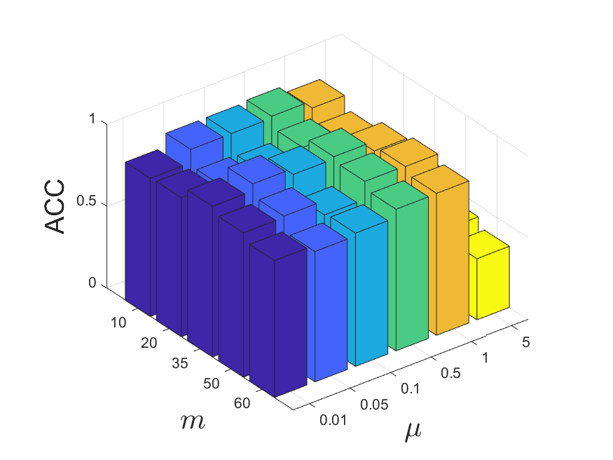
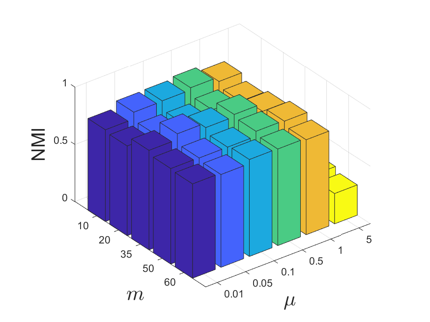
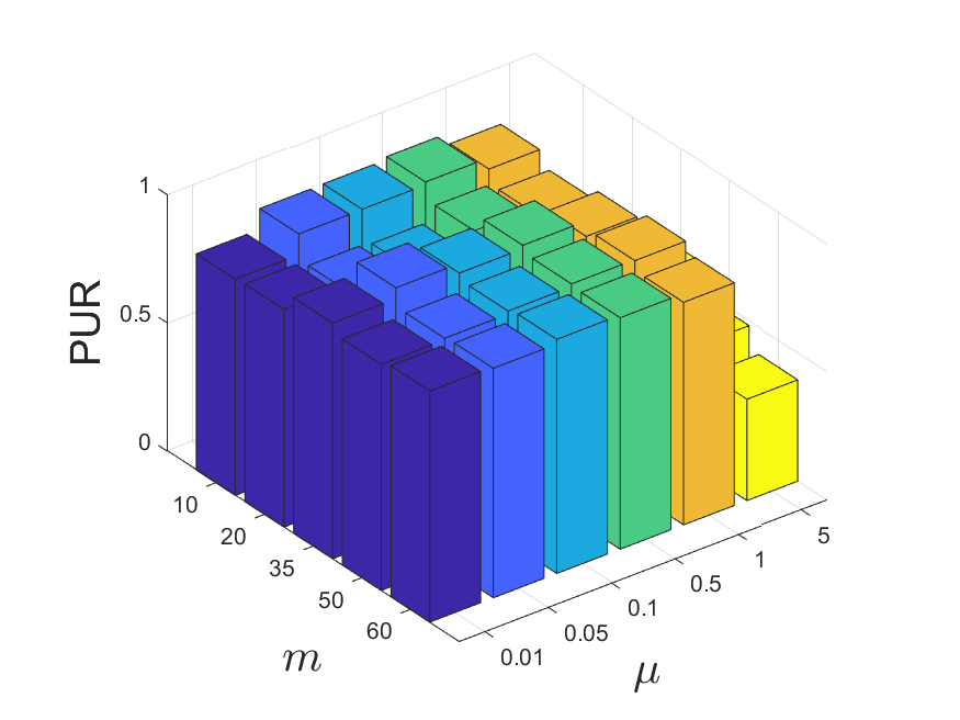
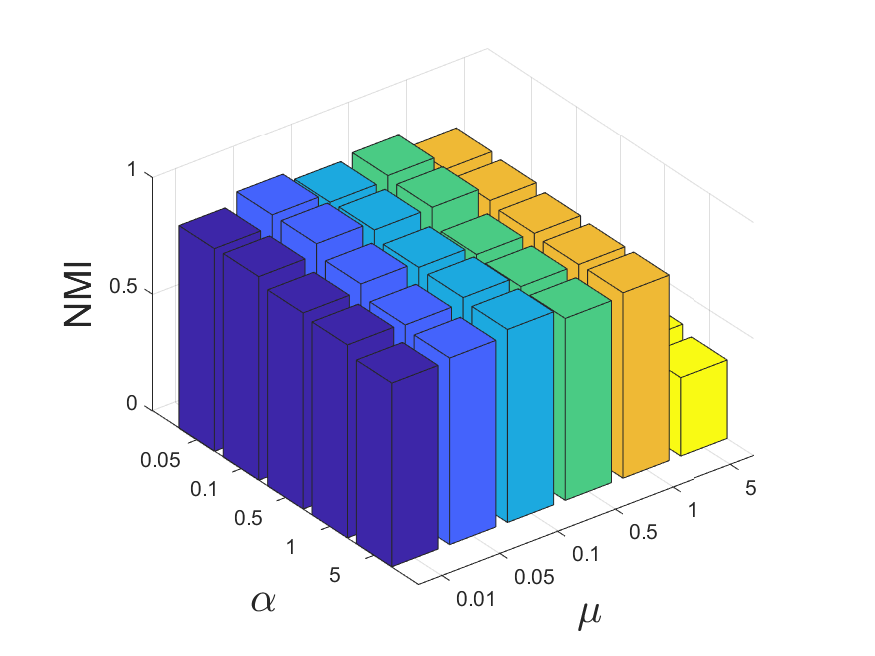
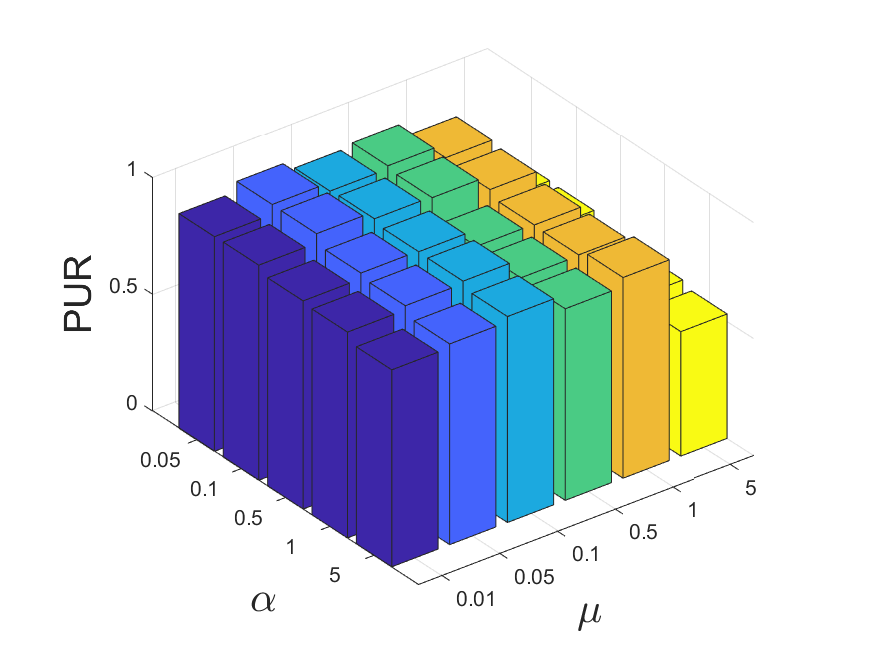
Figure 1: The parameter sensitivity on Handwritten.

For heterogeneous graph data, we find that $\alpha$ has little influence on the results, thus we fix it to $20$. DBLP, for instance, we find that its performance is robust to the number $m$ according to Fig. 2.

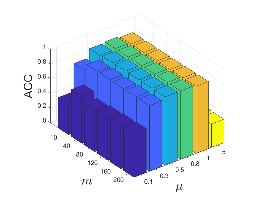
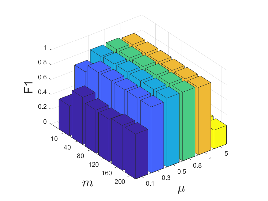
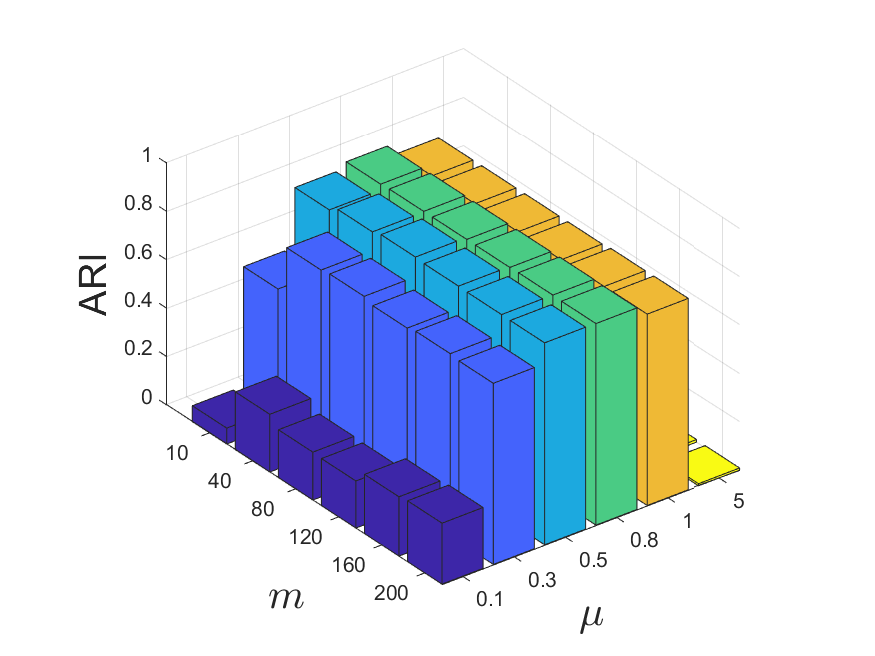
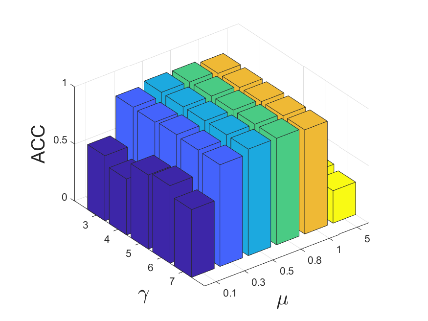
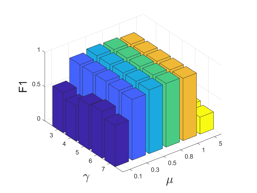
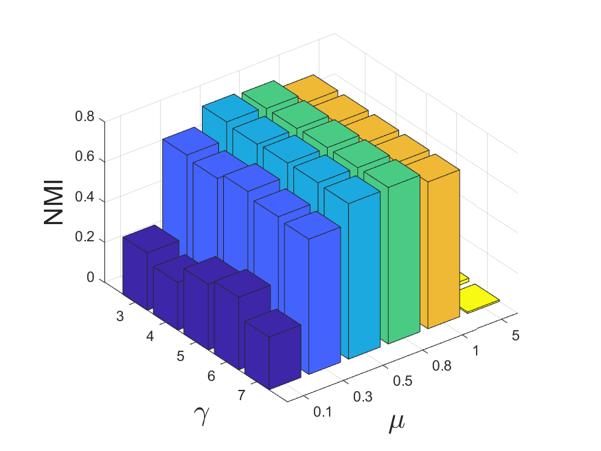
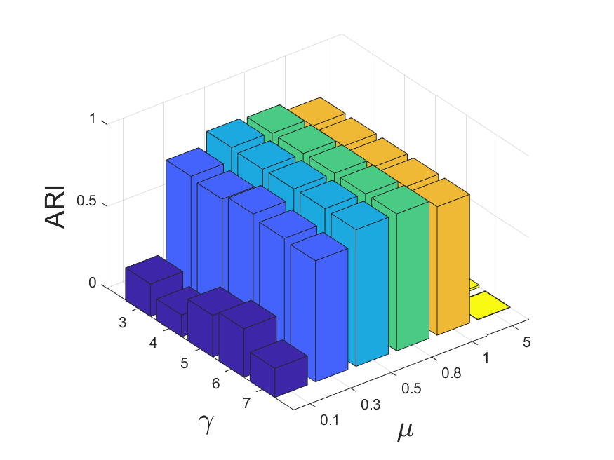
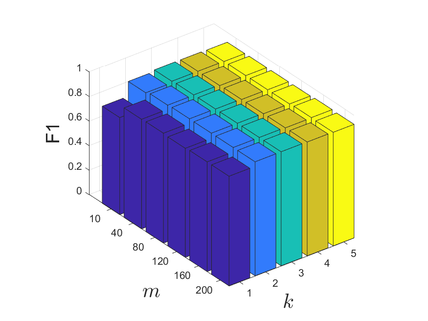
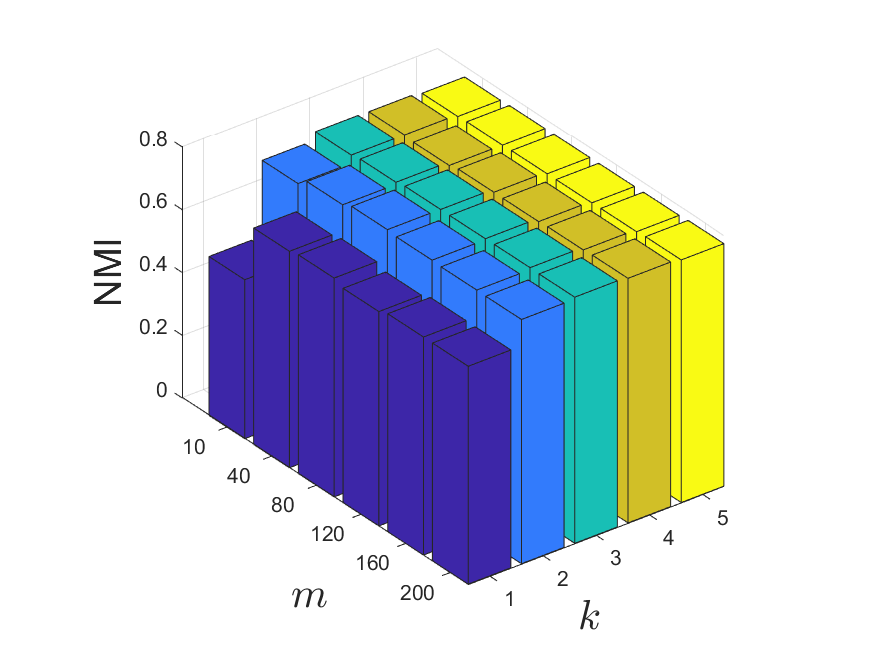
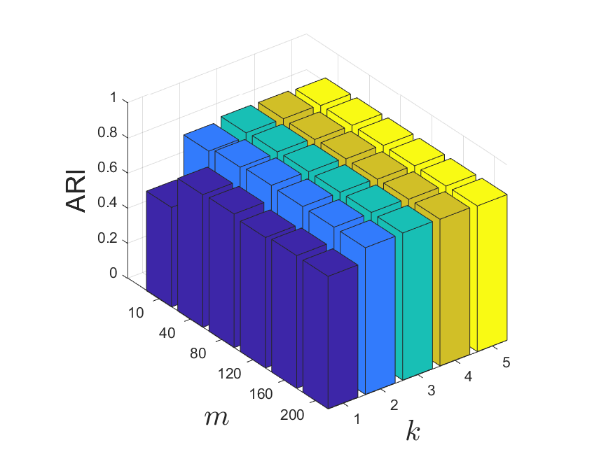
Figure 2: The parameter sensitivity on DBLP.

Therefore, we search $m$ in the range of 80 to 120 on all datasets. Besides, it is obvious that the performance is not sensitive to sampling parameter $\gamma$, thus we fix it to 2. Regarding filter order, $k=3$ or $k=4$ often generates good performance. If $k$ is too large, the resulted representation will become too smooth, which makes data points difficult to distinguish. In addition, we can see that either large or small $\mu$ are not good. Since different data have different levels of noise, the value of $\mu$ heavily depends on the specific dataset.

To intuitively see the effect of $\mu$, we fix $k=1$ and display the 2D embedding of DBLP using $t$-SNE algorithm van2008visualizing . As shown in Fig. 3, a proper $\mu$ could produce a clustering-friendly representation.

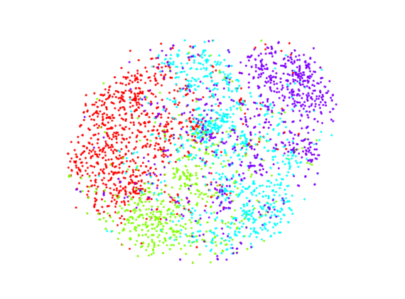
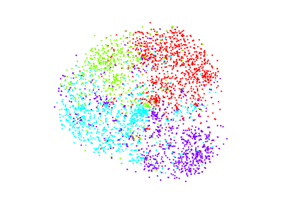
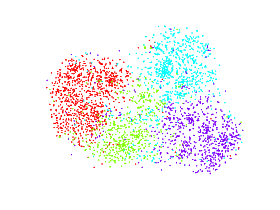
raw feature	$\mu=0.3$	$\mu=0.5$
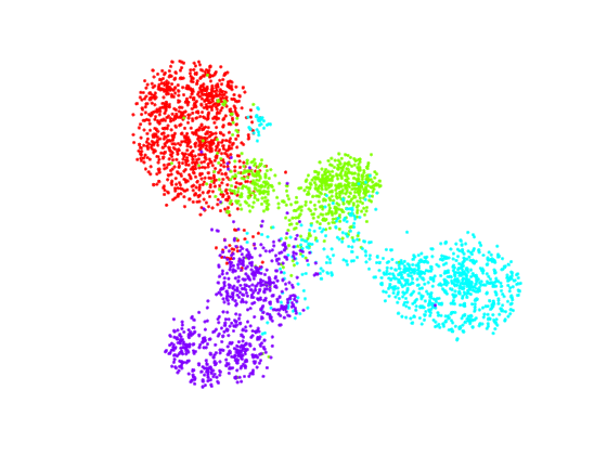
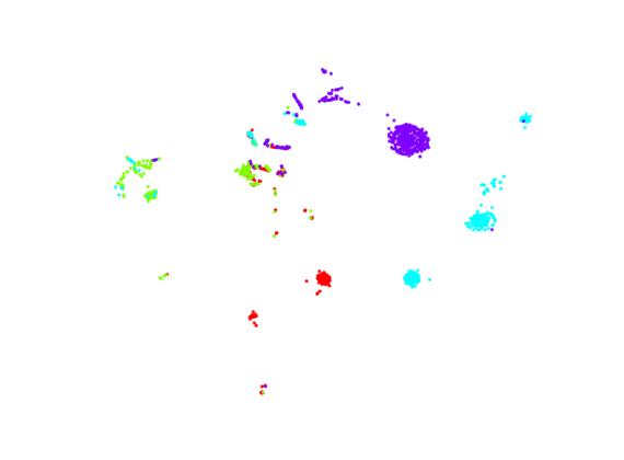
$\mu=0.6$	$\mu=0.8$	$\mu=1.0$

Figure 3: The 2D visualization of DBLP using t-SNE.

For example, points from different categories are well separated when $\mu=0.6$ or 0.8. When $\mu=1$, the cluster structure becomes vague.

5 Conclusion

In this paper, we propose a scalable graph filter-based multi-view clustering method. It is general to handle both feature and graph data. There are two novel components in the proposed framework. First, an adaptive graph filter is introduced to remove high-frequency noise. Second, a novel sampling mechanism is designed to improve the quality of anchors. Comprehensive experiments demonstrate that the proposed method is not only effective but also efficient. In particular, our proposed method surpasses several state-of-the-art deep neural networks based methods.

Compliance with ethical standards

Conflict of interest In compliance with ethical standards as researchers, the authors have no potential conflict of interest. The authors certify that they have no affiliations with or involvement in any organization or entity with any financial interest or non-financial interest in the subject matter or materials discussed in this manuscript.

References

- (1) Kang, Z., Lin, Z., Zhu, X., Xu, W.: Structured graph learning for scalable subspace clustering: From single-view to multi-view. IEEE Transactions on Cybernetics (2021)
- (2) Chao, G., Sun, S., Bi, J.: A survey on multi-view clustering. IEEE Transactions on Artificial Intelligence (2021)
- (3) Hou, C., Zeng, L.L., Hu, D.: Safe classification with augmented features. IEEE transactions on pattern analysis and machine intelligence 41(9), 2176–2192 (2018)
- (4) Yu, Q., Xu, W., Wu, Y., Zhang, H.: Learning to collocate fashion items from heterogeneous network using structural and textual features. In: International Conference on Neural Computing for Advanced Applications, pp. 166–180. Springer (2021)
- (5) Huang, S., Kang, Z., Xu, Z., Liu, Q.: Robust deep k-means: An effective and simple method for data clustering. Pattern Recognition 117, 107996 (2021)
- (6) Zhu, X., Zhu, Y., Zheng, W.: Spectral rotation for deep one-step clustering. Pattern Recognition 105, 107175 (2020)
- (7) Mi, Y., Ren, Z., Xu, Z., Li, H., Sun, Q., Chen, H., Dai, J.: Multi-view clustering with dual tensors. Neural Computing and Applications pp. 1–12 (2022)
- (8) Liu, Y.: Refined learning bounds for kernel and approximate -means. Advances in Neural Information Processing Systems 34 (2021)
- (9) Chen, M.S., Huang, L., Wang, C.D., Huang, D.: Multi-view clustering in latent embedding space. In: Proceedings of the AAAI conference on artificial intelligence, vol. 34, pp. 3513–3520 (2020)
- (10) Kumar, A., Daumé, H.: A co-training approach for multi-view spectral clustering. In: Proceedings of the 28th international conference on machine learning (ICML-11), pp. 393–400 (2011)
- (11) Kumar, A., Rai, P., Daume, H.: Co-regularized multi-view spectral clustering. Advances in neural information processing systems 24, 1413–1421 (2011)
- (12) Wang, H., Yang, Y., Zhang, X., Peng, B.: Parallel multi-view concept clustering in distributed computing. Neural Computing and Applications 32(10), 5621–5631 (2020)
- (13) Liu, X.: Incomplete multiple kernel alignment maximization for clustering. IEEE Transactions on Pattern Analysis and Machine Intelligence (2021)
- (14) Kang, Z., Zhao, X., Shi, Peng, C., Zhu, H., Zhou, J.T., Peng, X., Chen, W., Xu, Z.: Partition level multiview subspace clustering. Neural Networks 122, 279–288 (2020)
- (15) Zhang, C., Hu, Q., Fu, H., Zhu, P., Cao, X.: Latent multi-view subspace clustering. In: Proceedings of the IEEE conference on computer vision and pattern recognition, pp. 4279–4287 (2017)
- (16) Li, Z., Wang, Q., Tao, Z., Gao, Q., Yang, Z.: Deep adversarial multi-view clustering network. In: IJCAI, pp. 2952–2958 (2019)
- (17) Fan, S., Wang, X., Shi, C., Lu, E., Lin, K., Wang, B.: One2multi graph autoencoder for multi-view graph clustering. In: Proceedings of The Web Conference 2020, pp. 3070–3076 (2020)
- (18) Cheng, J., Wang, Q., Tao, Z., Xie, D.Y., Gao, Q.: Multi-view attribute graph convolution networks for clustering. In: IJCAI, pp. 2973–2979 (2020)
- (19) Nie, F., Li, J., Li, X.: Parameter-free auto-weighted multiple graph learning: A framework for multiview clustering and semi-supervised classification. In: International Joint Conference on Artificial Intelligence, pp. 1881–1887 (2016)
- (20) Brbić, M., Kopriva, I.: Multi-view low-rank sparse subspace clustering. Pattern Recognition 73, 247–258 (2018)
- (21) Xia, R., Pan, Y., Du, L., Yin, J.: Robust multi-view spectral clustering via low-rank and sparse decomposition. In: Proceedings of the AAAI conference on artificial intelligence, vol. 28 (2014)
- (22) Nie, F., Li, J., Li, X., et al.: Self-weighted multiview clustering with multiple graphs. In: IJCAI, pp. 2564–2570 (2017)
- (23) Wang, X., Lei, Z., Guo, X., Zhang, C., Shi, H., Li, S.Z.: Multi-view subspace clustering with intactness-aware similarity. Pattern Recognition 88, 50–63 (2019)
- (24) Kang, Z., Zhou, W., Zhao, Z., Shao, J., Han, M., Xu, Z.: Large-scale multi-view subspace clustering in linear time. In: Proceedings of the AAAI Conference on Artificial Intelligence, vol. 34, pp. 4412–4419 (2020)
- (25) Chen, P., Liu, L., Ma, Z., Kang, Z.: Smoothed multi-view subspace clustering. In: International Conference on Neural Computing for Advanced Applications, pp. 128–140. Springer (2021)
- (26) Liu, W., Chen, P.Y., Yeung, S., Suzumura, T., Chen, L.: Principled multilayer network embedding. In: 2017 IEEE International Conference on Data Mining Workshops (ICDMW), pp. 134–141. IEEE (2017)
- (27) Zhang, H., Qiu, L., Yi, L., Song, Y.: Scalable multiplex network embedding. In: IJCAI, vol. 18, pp. 3082–3088 (2018)
- (28) Wang, X., Ji, H., Shi, C., Wang, B., Ye, Y., Cui, P., Yu, P.S.: Heterogeneous graph attention network. In: The World Wide Web Conference, pp. 2022–2032 (2019)
- (29) Lin, Z., Kang, Z.: Graph filter-based multi-view attributed graph clustering. In: Proceedings of the Thirtieth International Joint Conference on Artificial Intelligence, IJCAI-21, pp. 2723–2729 (2021)
- (30) Lin, Z., Kang, Z., Zhang, L., Tian, L.: Multi-view attributed graph clustering. IEEE Transactions on Knowledge and Data Engineering (2021)
- (31) Dong, X., Thanou, D., Rabbat, M., Frossard, P.: Learning graphs from data: A signal representation perspective. IEEE Signal Processing Magazine 36(3), 44–63 (2019)
- (32) Pan, E., Kang, Z.: Multi-view contrastive graph clustering. Advances in Neural Information Processing Systems 34 (2021)
- (33) Ma, Z., Kang, Z., Luo, G., Tian, L., Chen, W.: Towards clustering-friendly representations: Subspace clustering via graph filtering. In: Proceedings of the 28th ACM International Conference on Multimedia, pp. 3081–3089 (2020)
- (34) Lv, J., Kang, Z., Lu, X., Xu, Z.: Pseudo-supervised deep subspace clustering. IEEE Transactions on Image Processing 30, 5252–5263 (2021)
- (35) Zhang, Z., Sun, Y., Wang, Y., Zhang, Z., Zhang, H., Liu, G., Wang, M.: Twin-incoherent self-expressive locality-adaptive latent dictionary pair learning for classification. IEEE Transactions on Neural Networks and Learning Systems 32(3), 947–961 (2020)
- (36) Nie, F., Wang, X., Jordan, M., Huang, H.: The constrained laplacian rank algorithm for graph-based clustering. In: Proceedings of the AAAI conference on artificial intelligence, vol. 30 (2016)
- (37) Tang, J., Qu, M., Wang, M., Zhang, M., Yan, J., Mei, Q.: Line: Large-scale information network embedding. In: Proceedings of the 24th international conference on world wide web, pp. 1067–1077 (2015)
- (38) Kipf, T.N., Welling, M.: Variational graph auto-encoders. In: NIPS Workshop on Bayesian Deep Learning (2016)
- (39) Van der Maaten, L., Hinton, G.: Visualizing data using t-sne. Journal of machine learning research 9(11) (2008)