An implicit, conservative and asymptotic-preserving electrostatic particle-in-cell algorithm for arbitrarily magnetized plasmas in uniform magnetic fields

Abstract

We introduce a new electrostatic particle-in-cell algorithm capable of using large timesteps compared to particle gyro-period under a uniform external magnetic field. The algorithm extends earlier electrostatic fully implicit PIC implementations with a new asymptotic-preserving particle-push scheme that allows timesteps much larger than particle gyroperiods. In the large-timestep limit, the integrator preserves all particle drifts, while recovering the full orbit for small timesteps. The scheme allows for a seamless, efficient treatment of particles with coexisting magnetized and unmagnetized species, and conserves energy and charge exactly without spoiling implicit solver performance. We demonstrate by numerical experiment with several problems of variable species magnetization (diocotron instability, modified two-stream instability, and drift instability) that orders of magnitude wall-clock-time speedups vs. the standard fully implicit electrostatic PIC algorithm are possible without sacrificing solution accuracy.

1 Introduction

Implicit particle-in-cell (PIC) algorithms (see e.g. Refs. [1, 2, 3, 4, 5] and references therein for recent implementations) may not be limited by the stability CFL timestep constraints of explicit PIC algorithms, and therefore hold much potential for more efficient kinetic plasma simulations. The fully implicit nonlinear PIC variety [1, 3, 4] is unconditionally stable, achieves simultaneous energy and charge conservation, ensuring long-term simulation fidelity by employing particle sub-cycling (a multirate integration approach), and enforcing nonlinear convergence of the particle-field system. The efficiency gains of implicit over explicit PIC reported in the literature [1, 2, 3, 4] originates largely from using large spatial cells (assuming constant number of particles per cell), but not from their ability to use large timesteps, due to the particle subcycling strategy needed to capture orbits accurately. Moreover, simultaneous energy and charge conservation demanded that particles do not step over cell faces in a single substep [1], requiring frequent orbit interruptions and nonlinear convergence for the orbit equations at each substep. The cost of particle subcycling in fully implicit PIC algorithms is particularly vexing in the context of strongly magnetized plasmas, where large gyrofrequencies will force commensurately small timesteps for accuracy. To make these methods competitive, an orbit integration strategy that can accurately step over the gyroperiod is needed.

Large timesteps compared to the gyroperiod (i.e., $\omega_{c}\Delta t\apprge 1$) can be used for the integration of the particle orbit equations without accuracy loss under certain conditions. This has been demonstrated for the explicit Boris particle-orbit integrator (“pusher” for short) [6] as well as implicit ones [7, 8]. These approaches capture most (if not all) zeroth- and first-order drifts of the guiding-center motion accurately, including the $\mathbf{E}\times\mathbf{B}$ drift, polarization drift, etc. However, significant drawbacks remain. In the explicit pusher, the gyroradius $\rho_{c}$ scales with $\Delta t$ (i.e., $\rho_{c}\sim O(v_{\perp}\Delta t)$, with $v_{\perp}$ the gyro-speed), which leads to significant orbit errors in $\rho_{c}$ when $\omega_{c}\Delta t\apprge 2$ [6]. Consequently, in practice one must limit the timestep to a fraction of the gyro-period for accuracy [9]. De-centered implicit pushers [7] introduce numerical damping that not only reduces the gyro-radius in time, but also breaks energy conservation, and are therefore unsuitable for long-term simulations. Time-centered Crank-Nicolson (CN) orbit integration schemes, however, show much promise. The CN scheme preserves the gyro-radius exactly, enables exact energy conservation, and retains the drift motions that persist at zero gyro-radius except for $\nabla B$ drifts, which require additional terms. In Ref. [8], a $\nabla B$ force was added to a CN integrator to account for the $\nabla B$ drift, but at the expense of energy conservation, allowing the magnetic field to do work on particles. More recent work [10] has shown that $\nabla B$-drift terms can be added to CN in a energy-conserving manner. We refer the reader to Ref. [10] for a discussion of the method, and for a more detailed accuracy comparison between various pushers.

There has been much renewed interest in PIC schemes for strong magnetization regimes, and in particular in the development of asymptotic preserving (AP) [11, 12, 13, 14] and uniformly accurate (UA) [15, 16, 17] methods. While AP schemes ensure numerical convergence to the asymptotic solution in the strongly magnetized regime, UA schemes seek numerical accuracy that is independent of the value of the magnetization, which is a stronger requirement. However, to date, UA schemes are restricted to either uniform magnetic fields [15, 16], or spatially varying but with uniform magnitude [17] (which removes the impact of the $\nabla B$ force on the long-time behavior of the system). Of particular relevance to this study is the approach proposed in Ref. [12], where an AP PIC scheme is constructed with an additional force term in the particle orbit equations, very similar to that proposed in Ref. [8], but again without strict conservation of energy.

In this study, we demonstrate the feasibility of an AP [18] implicit PIC algorithm that can employ particle substeps orders of magnitude larger than the gyroperiod without accuracy degradation or loss of strict conservation properties, and as a result is orders-of-magnitude faster than the subcycled fully implicit PIC variety for strongly magnetized plasmas [1]. For simplicity, we consider electrostatic collisionless plasmas in the presence of uniform magnetic fields. For these plasmas, CN captures all relevant drifts, and therefore can provide the basis for the present study. When implemented with a novel cell-crossing scheme that is both efficient and energy- and charge-conserving (similar in concept to that proposed in [19] for Vlasov-Maxwell PIC), the AP CN scheme proposed here delivers accurate and efficient kinetic simulations using large timesteps (i.e., $\omega_{ce}\Delta t\gg 1$) but still compatible with dynamical time scales of interest. Moreover, since the numerical gyro-frequency ($\hat{\omega}_{ce}$) decreases with the timestep according to the solution of $\hat{\omega}_{ce}\Delta t/2=\mathrm{atan}(\omega_{ce}\Delta t/2)$ [6, 10], it can become much smaller than the physical $\omega_{ce}$ for large $\Delta t$, effectively eliminating the numerical stiffness from Bernstein waves [20]. The resulting algorithm overcomes the particle-integration bottleneck of the standard nonlinear implicit PIC for strongly magnetized plasmas without needing to resolve the gyro-frequency.

The rest of the paper is organized as follows. Section 2 introduces the method employed in this study. The numerical implementation is described in Sec. 3. Section 4 demonstrates the effectiveness of the proposed algorithm with several electrostatic PIC tests. Finally, we conclude in Sec. 5.

2 Methodology

We consider next the key components of our AP particle-in-cell algorithm including particle substepping and orbit averaging, treatment of reflective boundaries, field solve, and enforcement of strict energy and charge conservation properties.

To begin, we intend to solve the electrostatic Vlasov-Ampere (VA) system for the electrostatic potential $\phi$ given by:

$$\epsilon_{0}\frac{\partial\nabla^{2}\phi}{\partial t} = \nabla\cdot\mathbf{j},$$ (1)

$$\mathbf{j}(\mathbf{x},t) = \sum_{\alpha}q_{\alpha}\int d\mathbf{v}\mathbf{v}f_{\alpha}(\mathbf{x},\mathbf{v},t),$$ (2)

$$\partial_{t}f_{\alpha}+\mathbf{v}\cdot\nabla f_{\alpha}+\frac{q_{\alpha}}{m_{\alpha}}\left(-\nabla\phi+\mathbf{v}\times\mathbf{B}_{0}\right)\cdot\nabla_{v}f_{\alpha} = 0.$$ (3)

Assuming the usual particle ansatz for the species particle distribution function, $f_{\alpha}\approx\sum_{p\in\alpha}w_{p}\delta(\mathbf{x}-\mathbf{x}_{p}(t))\delta(\mathbf{v}-\mathbf{v}_{p}(t))$, gives the particle closure for the current density:

$$\mathbf{j}(\mathbf{x},t) = \sum_{p}q_{p}w_{p}\mathbf{v}_{p}(t)\delta(\mathbf{x}-\mathbf{x}_{p}(t)),$$ (4)

$$\frac{dw_{p}}{dt}=0 \frac{d\mathbf{x}_{p}}{dt}=\mathbf{v}_{p}\,\,\,\,;\,\,\,\,\frac{d\mathbf{v}_{p}}{dt}=\frac{q_{p}}{m_{p}}\left(-\nabla\phi+\mathbf{v}\times\mathbf{B}_{0}\right).$$ ; (5)

In this study, $\mathbf{B}_{0}$ is considered uniform. These equations can be discretized with a multirate implicit formulation that conserves local charge and total energy exactly, as described in Refs. [1, 3, 4]. However, by design, the multirate particle integrator in the references must resolve the local gyrofrequency for accuracy, incurring significant inefficiencies for strongly magnetized plasmas. The purpose of this study is to generalize these implicit algorithms to be able to use arbitrary timesteps with respect to the gyrofrequency. In the very large gyrofrequency limit, $\omega_{ce}\Delta t\gg 1$, the particle motion is described by its gyrocenter, and the current density moment becomes the gyrocenter current contribution plus a magnetization current [21, 22]:

$$\mathbf{j}=\mathbf{j}_{gc}+\nabla\times\mathbf{M},$$ (6)

where $\mathbf{j}_{gc}$ is the gyro-center current. Since the magnetization current is solenoidal, it follows that $\nabla\cdot\mathbf{j}=\nabla\cdot\mathbf{j}_{gc}$, and therefore the field equation (Eq. 1) remains invariant in the strongly magnetized regime. This property renders the electrostatic PIC system, Eqs. 1, 4, and 5, ideally suited for exploration of asymptotic preserving discretizations of the particle-field equations.

2.1 Particle sub-stepping and orbit-averaging

We seek to employ very large timesteps compared to the gyroperiod for advancing particles using a CN integrator (see Refs. [1, 3, 4] and also the discussion below). By doing so, the particle orbits do not resolve the gyromotion, but are still able to capture low-order drift motions while preserving the Larmor radius [10]. Specifically, as shown in the reference, CN without modification can capture all the low-order drifts such as $E\times B$ drift, polarization drift, curvature drift, etc., except for the magnetic drift (which does not appear for a constant magnetic field, the case considered in this study).

In earlier energy-conserving implicit PIC implementations [1, 3, 4], automatic charge conservation was enforced without loss of energy conservation by having particles stop at cell faces. While this approach affords significant accuracy improvements vs. non-conserving strategies, its disadvantage is that the number of cell crossings (and therefore of substeps) increases with the size of the implicit timestep. The cost of the orbit integration grows accordingly, thus offsetting any potential efficiency gains of the implicit scheme from large timesteps.

To remove this limitation and improve efficiency without sacrificing accuracy, we introduce in this study a new CN mover without the requirement that each particle stops at cell faces, while still enforcing discrete charge and energy conservation. The key innovation of the approach is to allow orbit substeps that can be much larger than the cell size, assuming each substep is straight with a constant velocity across the whole substep. For an implicit field timestep $\Delta t$, the orbit equations are solved for each orbit substep $\Delta\tau^{\nu}$ ($\Delta t\geq\Delta\tau^{\nu}>0$, where $\nu$ denotes the substep number), which is now determined according to physical considerations beyond the cell size (e.g., see Ref. [10]). Charge and energy conservation are still enforced strictly by keeping track of segments (defined as the part of a substep that is within a cell) crossed by the straight substep, a procedure done on the fly in a very efficient manner. Accordingly, the average cost of each particle orbit push becomes largely independent of the size of the implicit field timestep, translating the efficiency savings directly into wall-clock-time savings. In what follows, we outline the basic particle sub-stepping and orbit-averaging techniques proposed in this study.

We begin with the implicit CN discretization for the particle orbit equations used for each substep $\nu$,

$$\mathbf{x}_{p}^{\nu+1} =\mathbf{x}_{p}^{\nu}+\Delta\tau_{p}^{\nu}\mathbf{v}_{p}^{\nu+1/2},$$ (7)

$$\mathbf{v}_{p}^{\nu+1} =\mathbf{v}_{p}^{\nu}+\frac{\Delta\tau_{p}^{\nu}q_{p}}{m_{p}}\left(\mathbf{E}_{p}^{\nu+1/2}+\mathbf{v}_{p}^{\nu+1/2}\times\mathbf{B}_{0}\right),$$ (8)

where $q_{p}$, $m_{p}$ are the particle charge and mass, the integer superscript $\nu$ denotes the substep time level, $\mathbf{v}_{p}^{\nu+1/2}=(\mathbf{v}_{p}^{\nu}+\mathbf{v}_{p}^{\nu+1})/2$, $\mathbf{B}_{0}$ is a constant external magnetic field (temporally and spatially), $\mathbf{E}_{p}^{\nu+1/2}$ is the segment-averaged particle electric field (to be specified), and $\Delta\tau_{p}^{\nu}$ is the particle sub-timestep. Note that, for any particle $p$, $\sum_{\nu\in n}\Delta\tau_{p}^{\nu}=\Delta t$, where the summation is over all substeps in the timestep $n$. Equation 8 can be analytically inverted [23] to give:

$$\mathbf{a}_{p} =\mathbf{v}_{p}^{\nu}+\alpha_{p}\mathbf{E}_{p}^{\nu+1/2},$$ (9)

$$\mathbf{v}_{p}^{\nu+1/2} ={\color[rgb]{1,0,0}\frac{\mathbf{a}_{p}+\alpha_{p}\mathbf{a}_{p}\times\mathbf{B}_{0}+\alpha_{p}^{2}(\mathbf{a}_{p}\cdot\mathbf{B}_{0})\mathbf{B}_{0}}{1+(\alpha_{p}B_{0})^{2}},}$$ (10)

$$\mathbf{x}_{p}^{\nu+1} =\mathbf{x}_{p}^{\nu}+\Delta\tau_{p}^{\nu}\mathbf{v}_{p}^{\nu+1/2},$$ (11)

$$\mathbf{v}_{p}^{\nu+1} =2\mathbf{v}_{p}^{\nu+1/2}-\mathbf{v}_{p}^{\nu},$$ (12)

where $\alpha_{p}=0.5\Delta\tau_{p}^{\nu}q_{p}/m_{p}$. Here, we have assumed that, during the (possibly very large compared to the gyroperiod) sub-timestep $\Delta\tau_{p}^{\nu}$, the velocity is constant and the trajectory is a straight line (see Eq. 11 and Fig. 1). Since the right-hand-side of Eqs. 10-11 depends on both $\mathbf{x}_{p}^{\nu+1}$ and $\mathbf{v}_{p}^{\nu+1/2}$, a nonlinear iteration is needed. However, the analytically inverted form in Eqs. 9-12 is asymptotically well posed for large timesteps ($\alpha_{p}B_{0}=\Delta\tau_{p}\omega_{c,p}\gg 1$), and a simple Picard iteration generally converges to very tight tolerances in very few iterations [3, 24].

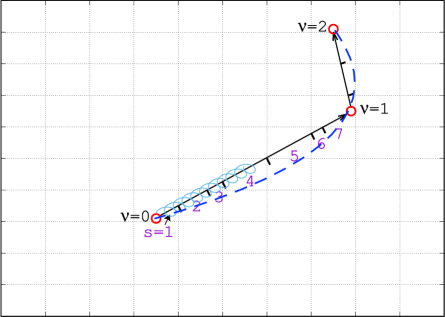
Figure 1: An illustration of a two-substep particle move. The substeps are between for $\nu=0,1$ and $\nu=1,2$, each of which is a straight line. Within each substep, the orbit line is further divided into segments separated by cell boundaries, which are labeled by $s=1,2$, etc. as shown for the first substep. The division into cell segments is done for each substep. In our algorithm, depending on local conditions, it is possible that a given substep approximates either an asymptotic guiding-center orbit (e.g., the solid spiral orbit) or a part of a well-resolved orbit (e.g., the dashed curve).

We now specify the particle electric field $\mathbf{E}_{p}^{\nu+1/2}$, which is obtained by segment-averaging along the straight-line orbit during the particle substep $\nu$ as:

$$\mathbf{E}_{p}^{\nu+\nicefrac{{1}}{{2}}}=\sum_{h}\mathbf{E}_{h}^{n+\nicefrac{{1}}{{2}}}\cdot\left\langle\bar{\bar{\mathbf{S}}}(\mathbf{x}_{h}-\mathbf{x}_{p}^{s+\nicefrac{{1}}{{2}}})\right\rangle_{p}^{\nu},$$ (13)

where $h=(i,j,k)$ is the mesh index,

$$\mathbf{E}_{h}^{n+\nicefrac{{1}}{{2}}}=\frac{\mathbf{E}_{h}^{n+1}+\mathbf{E}_{h}^{n}}{2}$$ (14)

is the mid-time electric field, defined at cell faces, the superscript $s$ denotes a segment of length $\Delta\mathbf{x}_{p}^{s}$ on the straight-line orbit segment $\Delta\mathbf{x}_{p}^{\nu}=\mathbf{x}_{p}^{\nu+1}-\mathbf{x}_{p}^{\nu}$ (see Fig. 1), and $\mathbf{x}_{p}^{s+\nicefrac{{1}}{{2}}}$ is the mid-point of $\Delta\mathbf{x}_{p}^{s}$. In Eq. 13, we have introduced the segment-average operator of the shape function $\left\langle\bar{\bar{\mathbf{S}}}(\mathbf{x}_{h}-\mathbf{x}_{p}^{s+\nicefrac{{1}}{{2}}})\right\rangle_{p}^{\nu}$ along the $\nu$-substep of the orbit of particle $p$, which will be defined in detail below. In each segment $[\mathbf{x}_{p}^{s},\mathbf{x}_{p}^{s+1}]$, the shape function dyad at cell faces is evaluated at $\mathbf{x}_{p}^{s+\nicefrac{{1}}{{2}}}$ as:

$$\bar{\bar{\mathbf{S}}}(\mathbf{x}_{i,j,k}-\mathbf{x}_{p}^{s+\nicefrac{{1}}{{2}}}) = \mathbf{i}\otimes\mathbf{i}\,\,S_{1}(x_{i+\nicefrac{{1}}{{2}}}-x_{p}^{s+\nicefrac{{1}}{{2}}})\mathcal{\mathbb{S}}_{22,jk}^{s+\nicefrac{{1}}{{2}}}(y_{p},z_{p})$$

$$+ \mathbf{j}\otimes\mathbf{j}\,\,S_{1}(y_{j+\nicefrac{{1}}{{2}}}-y_{p}^{s+\nicefrac{{1}}{{2}}})\mathcal{\mathbb{S}}_{22,ik}^{s+\nicefrac{{1}}{{2}}}(z_{p},x_{p})$$

$$+ \mathbf{k}\otimes\mathbf{k}\,\,S_{1}(z_{k+\nicefrac{{1}}{{2}}}-z_{p}^{s+\nicefrac{{1}}{{2}}})\mathcal{\mathbb{S}}_{22,ij}^{s+\nicefrac{{1}}{{2}}}(x_{p},y_{p}),$$

where $\mathbf{i},\mathbf{j},\mathbf{k}$ are unit vectors in the $x$, $y$, $z$ directions, respectively, $\otimes$ denotes tensor product, $S_{1}(x_{i+\nicefrac{{1}}{{2}}}-x_{p}^{s+\nicefrac{{1}}{{2}}})$ denotes linear B-spline shape function with $x_{i+\nicefrac{{1}}{{2}}}$ at cell faces, and

$$\mathcal{\mathbb{S}}_{22,jk}^{s+\nicefrac{{1}}{{2}}}(y,z)\equiv\frac{1}{3} \left[S_{2}(y_{j}-y^{s+1})S_{2}(z_{k}-z^{s+1})+\frac{S_{2}(y_{j}-y^{s})S_{2}(z_{k}-z^{s+1})}{2}\right.$$

$$\left.\>\;+\frac{S_{2}(y_{j}-y^{s+1})S_{2}(z_{k}-z^{s})}{2}+S_{2}(y_{j}-y^{s})S_{2}(z_{k}-z^{s})\right]$$ (16)

is defined with the explicit purpose of enforcing charge conservation [25], as will be shown below. In the last equation, $S_{2}(y_{j}-y^{s+1})$ is the quadratic B-spline shape function, with $y_{j}$ denoting a cell center (in $y$). The components of the segment-averaged shape function dyad $\left\langle\bar{\bar{\mathbf{S}}}(\mathbf{x}_{h}-\mathbf{x}_{p}^{s+\nicefrac{{1}}{{2}}})\right\rangle_{p}^{\nu}$ along the $\nu$ substep of the orbit of particle $p$ are defined as:

$$\mathbf{i}\cdot\left\langle\bar{\bar{\mathbf{S}}}(\mathbf{x}_{i,j,k}-\mathbf{x}_{p}^{s+\nicefrac{{1}}{{2}}})\right\rangle_{p}^{\nu}=\frac{\mathbf{i}}{\Delta x_{p}^{\nu}}\sum_{s\in\nu}S_{1}(x_{i+\nicefrac{{1}}{{2}}}-x_{p}^{s+\nicefrac{{1}}{{2}}})\mathcal{\mathbb{S}}_{22,jk}^{s+\nicefrac{{1}}{{2}}}(y_{p},z_{p})\Delta x_{p}^{s},$$ (17)

and similarly with $\mathbf{j}$ and $\mathbf{k}$ components. Here, the summation is over all segments that belong to the substep $\nu$.

As a result of the above gathering, $\mathbf{E}_{p}^{\nu+\nicefrac{{1}}{{2}}}$ is the segment-averaged electric field for the straight line $[\mathbf{x}_{p}^{\nu},\mathbf{x}_{p}^{\nu+1}]$ of substep $\nu$. The number of $\Delta\mathbf{x}_{p}^{s}$ segments is determined by the number of cell-crossings. The sub-timestep $\Delta\tau^{\nu}$ may be determined by a timestep estimator [1, 10], as discussed below. Similarly, by symmetry (required for strict energy conservation, as we show below), we obtain the segment-averaged current density at cell faces from:

$$\mathbf{j}_{h,p}^{\nu+\nicefrac{{1}}{{2}}}=\frac{q_{p}}{\Delta_{h}}\mathbf{v}_{p}^{\nu+\nicefrac{{1}}{{2}}}\cdot\left\langle\bar{\bar{\mathbf{S}}}(\mathbf{x}_{h}-\mathbf{x}_{p}^{s+\nicefrac{{1}}{{2}}})\right\rangle_{p}^{\nu},$$ (18)

where $\Delta_{h}$ denotes cell volume. It is worth noting that the proposed deposition scheme is similar to the one proposed by Esirkepov in Ref. [26], but we allow segment averaging over many cells (instead of just one in the reference), and we are limited to at most second-order B-splines (instead of arbitrary order).

2.2 Boundary treatment of reflective particles

Realistic finite-domain particle simulations will feature physical boundaries (e.g., walls), and therefore it is important to provide a mechanism to adapt the AP particle orbit integration in their presence. We consider here the case of perfectly reflecting walls, which do not spoil energy conservation [27] and are suitable to diagnose and demonstrate conservation properties. The treatment proposed here can be generalized to other boundary conditions (e.g., absorption, emission, etc.), if needed.

Given the particle sub-stepping strategy described above, it is natural and straightforward to include a boundary condition. This is because we can simply make one of the particle substeps end at the wall. This is done by iterating the particle EOM such that the particle ends at the wall when hitting it. For reflective boundary conditions, the normal velocity of the particle is flipped when the particle hits the wall. More specifically, if a particle is found to move beyond a wall, we resolve the full particle orbit with the substep computed as::

$$\Delta\tau_{p}^{\nu}=\textsf{min}\left(\Delta\tau_{p}^{\nu,*},\frac{x_{w}-x_{p}^{\nu}}{v_{px}^{\nu+\nicefrac{{1}}{{2}}}},\frac{y_{w}-y_{p}^{\nu}}{v_{py}^{\nu+\nicefrac{{1}}{{2}}}},\frac{z_{w}-z_{p}^{\nu}}{{\color[rgb]{1,0,0}v_{pz}^{\nu+\nicefrac{{1}}{{2}}}}}\right),$$ (19)

where $\Delta\tau_{p}^{\nu,*}$ is found from a timestep estimator (see Ref. [1] and also below). If any velocity component is zero, the particle will not move in that direction. Iterations of the particle EOM for that substep will carry on with the updated $\Delta\tau_{p}^{\nu}$ until convergence. In practice, we iterate Eqs. 9-11 to convergence, and if a particle intersects the boundary, its position for the end of that substep is placed at the wall according to Eq. 19. After convergence, we flip the sign of its normal component to the wall,

$$\mathbf{n}\cdot\mathbf{v}_{p}^{\nu+1}\rightarrow-\mathbf{n}\cdot\mathbf{v}_{p}^{\nu+1},$$

where $\mathbf{n}$ denotes the normal vector to the wall boundary, and the orbit integration continues as before.

When the particle is deemed close to the boundary, its substep $\Delta\tau^{\nu}$ is estimated to control the integration error of the Crank–Nicolson temporal scheme, which can be succinctly written as:

$$\hat{\mathbf{x}}^{\nu+1} =\mathbf{x}^{\nu}+\Delta\tau^{\nu}\frac{\hat{\mathbf{v}}^{\nu+1}+\mathbf{v}^{\nu}}{2},$$ (20)

$$\hat{\mathbf{v}}^{\nu+1} =\mathbf{v}^{\nu}+\Delta\tau^{\nu}\frac{\hat{\mathbf{a}}^{\nu+1}+\mathbf{a}^{\nu}}{2}.$$ (21)

Assuming that $\mathbf{a}(\tau)\approx\mathbf{a}^{\nu}+(d\mathbf{a}/d\tau)^{\nu}\tau$, we can re-write the equations as

$$\hat{\mathbf{x}}^{\nu+1}=\mathbf{x}^{\nu}+\mathbf{v}^{\nu}\Delta\tau^{\nu}+\frac{1}{2}\mathbf{a}^{\nu}(\Delta\tau^{\nu})^{2}+\frac{1}{4}(\frac{d\mathbf{a}}{d\tau})^{\nu}(\Delta\tau^{\nu})^{3}+\mathcal{O}((\Delta\tau^{\nu})^{4}).$$ (22)

Taylor-expanding the exact solution in time we obtain:

$$\mathbf{x}^{\nu+1}=\mathbf{x}^{\nu}+\mathbf{v}^{\nu}\Delta\tau^{\nu}+\frac{1}{2}\mathbf{a}^{\nu}(\Delta\tau^{\nu})^{2}+\frac{1}{6}(\frac{d\mathbf{a}}{d\tau})^{\nu}(\Delta\tau^{\nu})^{3}+\mathcal{O}((\Delta\tau^{\nu})^{4}).$$ (23)

The leading local truncation error is found by subtracting Eq. 23 and 22, yielding:

$$\mathcal{E}_{\Delta\tau}=\frac{1}{12}(\frac{d\mathbf{a}}{d\tau})^{\nu}(\Delta\tau^{\nu})^{3}.$$ (24)

Equation 24 is rearranged to find an estimate of $\Delta\tau^{\nu}$ as:

$$\Delta\tau^{\nu}=\left(\frac{12\mathcal{E}_{\Delta\tau}}{\left\|(d\mathbf{a}/d\tau)^{\nu}\right\|}\right)^{\frac{1}{3}},$$ (25)

where $\mathcal{E}_{\Delta\tau}$ is a user-provided local error tolerance (here we use $\mathcal{E}_{\Delta\tau}=0.01$). The rate of change of the acceleration needs to be estimated along the particle substep $\nu$. In this study, we predict it at the beginning of the substep by using Euler’s scheme with a tiny step $\delta\tau=10^{-8}$ to push the particle to a new location $\mathbf{x}_{E}$, and compute $(\frac{d\mathbf{a}}{d\tau})^{\nu}\simeq(\mathbf{a}(\mathbf{x}_{E})-\mathbf{a}^{\nu})/\delta\tau$. More sophisticated estimates that account for the change of $\mathbf{a}$ along the full substep may be needed in the future, and will be explored in future work.

2.3 Field solver

We find the electrostatic potential from Gauss’ law combined with the continuity equation [3, 4]:

$$\epsilon_{0}\frac{\partial\nabla^{2}\phi}{\partial t}-\nabla\cdot\mathbf{j}=0.$$ (26)

In discrete form, it reads:

$$\epsilon_{0}(\nabla_{h}^{2}\phi_{h}^{n+1}-\nabla_{h}^{2}\phi_{h}^{n})-\Delta t\nabla_{h}\cdot\bar{\mathbf{j}}_{h}^{n+1/2}=0,$$ (27)

which is the standard second-order time-domain finite-difference scheme on the Yee mesh (as in Ref. [4]), with $\phi_{h}$ defined at cell centers and components of $\bar{\mathbf{j}}_{h}$ colocated with the electric field ones (normal to faces). The orbit-averaged current density is obtained from:

$$\bar{\mathbf{j}}_{h}^{n+1/2}=\frac{1}{\Delta t}\sum_{p}\sum_{\nu\in n}\mathbf{j}_{h,p}^{\nu+\nicefrac{{1}}{{2}}}\Delta\tau_{p}^{\nu},$$ (28)

which can be expanded using Eq. 18 as:

$$\bar{\mathbf{j}}_{h}^{n+1/2} =\frac{1}{\Delta t}\sum_{p}\sum_{\nu\in n}\frac{q_{p}}{\Delta_{h}}\mathbf{v}_{p}^{\nu+\nicefrac{{1}}{{2}}}\cdot\left\langle\bar{\bar{\mathbf{S}}}(\mathbf{x}_{h}-\mathbf{x}_{p}^{s+\nicefrac{{1}}{{2}}})\right\rangle^{\nu}\Delta\tau_{p}^{\nu},$$

$$=\frac{1}{\Delta_{h}\Delta t}\sum_{p}\sum_{s\in n}q_{p}\Delta\mathbf{x}_{p}^{s}\cdot\bar{\bar{\mathbf{S}}}(\mathbf{x}_{h}-\mathbf{x}_{p}^{s+\nicefrac{{1}}{{2}}}),$$ (29)

where the double sum performs the average over all segments of all particles for the whole timestep. The electric field is obtained at integer time levels and cell faces by a central-difference face gradient:

$$\mathbf{E}_{h}=-\nabla_{h}\phi_{h}.$$ (30)

As is demonstrated in the next section, the discrete continuity equation

$$\rho_{h}^{n+1}-\rho_{h}^{n}+\Delta t\nabla_{h}\cdot\bar{\mathbf{j}}_{h}^{n+1/2}=0$$ (31)

is exactly satisfied when $\rho_{h}$ is defined as:

$$\rho_{h}=\sum_{p}\frac{q_{p}}{\Delta_{h}}S_{2}(x_{i+1/2}-x_{p})S_{2}(y_{j+1/2}-y_{p})S_{2}(z_{k+1/2}-z_{p}).$$ (32)

Therefore, up to the nonlinear tolerance, the discrete Gauss’s law follows from Eq. 27 and 31 as

$$\epsilon_{0}\nabla_{h}^{2}\phi_{h}^{n+1}=-\rho_{h}^{n+1},$$ (33)

for $n>0$ if it is satisfied at $n=0$.

2.4 Energy and charge conservation properties

We show that the proposed algorithm is energy- and charge-conserving as follows. For energy conservation, we prove that the discrete total energy (TE) is exactly conserved without energy sources, i.e.,

$$\left.\left(\mathrm{TE}\right)\right|_{n}^{n+1}=\left.\left(W_{E}+K\right)\right|_{n}^{n+1}=0,$$ (34)

where

$$W_{E}^{n}\equiv\frac{\epsilon_{0}}{2}\sum_{h}\bm{\Delta}_{h}(\mathbf{E}_{h}^{n})^{2},$$

and

$$K^{n}\equiv\frac{1}{2}\sum_{p}m_{p}(v_{p}^{n})^{2}.$$

This is shown as follows:

$$K^{n+1}-K^{n} =\sum_{p}m_{p}\frac{\mathbf{v}_{p}^{n+1}+\mathbf{v}_{p}^{n}}{2}(\mathbf{v}_{p}^{n+1}-\mathbf{v}_{p}^{n})$$

$$=\sum_{p}\cancel{m_{p}}\sum_{\nu\in n}\frac{\mathbf{v}_{p}^{\nu+1}+\mathbf{v}_{p}^{\nu}}{2}\cdot\left(\mathbf{E}_{p}^{\nu+1/2}+\frac{\mathbf{v}_{p}^{\nu+1}+\mathbf{v}_{p}^{\nu}}{2}\times\mathbf{B}_{0}\right)\frac{\Delta\tau^{\nu}q_{p}}{\cancel{m_{p}}}$$

$$=\sum_{p}\sum_{\nu\in n}\Delta\mathbf{x}_{p}^{\nu}q_{p}\sum_{h}\mathbf{E}_{h}^{n+\nicefrac{{1}}{{2}}}\cdot\left\langle\bar{\bar{\mathbf{S}}}(\mathbf{x}_{h}-\mathbf{x}_{p}^{s+\nicefrac{{1}}{{2}}})\right\rangle_{p}^{\nu}$$

$$=\sum_{h}\mathbf{E}_{h}^{n+\nicefrac{{1}}{{2}}}\cdot\bar{\mathbf{j}}_{h}^{n+1/2}\Delta_{h}\Delta t$$

$$=-\sum_{h}\nabla_{h}\phi_{h}^{n+\nicefrac{{1}}{{2}}}\cdot\bar{\mathbf{j}}_{h}^{n+1/2}\Delta_{h}\Delta t$$

$$=\sum_{h}\phi_{h}^{n+\nicefrac{{1}}{{2}}}\nabla_{h}\cdot\bar{\mathbf{j}}_{h}^{n+1/2}\Delta_{h}\Delta t$$

$$=\sum_{h}\phi_{h}^{n+\nicefrac{{1}}{{2}}}\epsilon_{0}\frac{\nabla_{h}^{2}\phi_{h}^{n+1}-\nabla_{h}^{2}\phi_{h}^{n}}{\cancel{\Delta t}}\Delta_{h}\cancel{\Delta t}$$

$$=-\frac{\epsilon_{0}}{2}\sum_{h}\left[(\mathbf{E}_{h}^{n+1})^{2}-(\mathbf{E}_{h}^{n})^{2}\right]\Delta_{h}$$

$$=-(W_{E}^{n+1}-W_{E}^{n}),$$

where we have used Eq. 8 for the second equality, Eq. 7, 13 and $\frac{\mathbf{v}^{\nu+1}+\mathbf{v}^{\nu}}{2}\cdot\left(\frac{\mathbf{v}^{\nu+1}+\mathbf{v}^{\nu}}{2}\times\mathbf{B}_{0}\right)=0$ for the third equality, Eq. 18, 28 for the fourth equality, Eq. 30 for fifth equality, integration by parts in the sixth equality, Eq. 27 for the seventh equality, integration by parts and Eq. 30 for the eighth equality, and we denote $\phi^{n+\nicefrac{{1}}{{2}}}\equiv(\phi^{n+1}+\phi^{n})/2$. Note that the discrete integration (or summation) by parts is satisfied for the standard second-order finite-difference schemes with periodic boundary conditions. We note that the derivation remains valid with a perfect-conductor boundary and reflecting particles. Assuming that we have perfect conductor walls confining the $y$-direction, with $\phi=0$ at both walls (i.e., no imposed electric field), all the above steps remain the same, including the summation by parts:

$$\sum_{j=0}^{N_{y}+1}\frac{\phi_{j}-\phi_{j-1}}{\Delta y}\bar{\mathfrak{j}}_{j}=-\sum_{j=0}^{N_{y}+1}\phi_{j}\frac{\bar{\mathfrak{j}}_{j}-\bar{\mathfrak{j}}_{j-1}}{\Delta y},$$

where we have used $\phi_{0}=\phi_{N_{y+1}}=0$. In multiple dimensions, the summation by parts is done for each dimension separately.

Regarding charge conservation, we show next that

$$\rho_{h}^{n+1}-\rho_{h}^{n}+\Delta t\nabla_{h}\cdot\mathbf{\bar{j}}_{h}^{n+1/2}=0.$$ (35)

It is sufficient that Eq. 35 be satisfied for each particle (the total follows when summing over all particle contributions), which can be written as

$$\sum_{\nu\in n}\left(\rho_{h,p}^{\nu+1}-\rho_{h,p}^{\nu}+\Delta\tau_{p}^{\nu}\nabla_{h}\cdot\mathbf{j}_{h,p}^{\nu+\nicefrac{{1}}{{2}}}\right)=0.$$ (36)

It is therefore sufficient for the continuity equation to be satisfied for each substep $\nu$, which may be written as

$$\sum_{s\in\nu}(\rho_{h,p}^{s+1}-\rho_{h,p}^{s})+\Delta\tau_{p}^{\nu}\nabla_{h}\cdot\mathbf{j}_{h,p}^{\nu+\nicefrac{{1}}{{2}}}=0,$$ (37)

where:

$$\rho_{h,p}^{s}=\frac{q_{p}}{\Delta_{h}}S_{2}(x_{i}-x_{p}^{s})S_{2}(y_{j}-y_{p}^{s})S_{2}(z_{k}-z_{p}^{s}),$$ (38)

and as before we use $s$ and $s+1$ for the start and end points of a segment $s$, respectively. Equation 37 can be expanded using Eq. 18 as:

$$\sum_{s\in\nu}\left[\rho_{h,p}^{s+1}-\rho_{h,p}^{s}+\nabla_{h}\cdot\frac{q_{p}}{\Delta_{h}}\bar{\bar{\mathbf{S}}}(\mathbf{x}_{h}-\mathbf{x}_{p}^{s+\nicefrac{{1}}{{2}}})\cdot\Delta\mathbf{x}_{p}^{s}\right]=0.$$ (39)

The expression in the square bracket describes the continuity equation for each segment $s$. Given Eqs. 38 and 2.1, 16, it follows that the continuity equation is exactly satisfied because:

$$(\rho_{h,p}^{s+1}-\rho_{h,p}^{s})\Delta_{h}/q_{p} = S_{2}(x_{i}-x_{p}^{s+1})S_{2}(y_{j}-y_{p}^{s+1})S_{2}(z_{k}-z_{p}^{s+1})$$ (40)

$$- S_{2}(x_{i}-x_{p}^{s})S_{2}(y_{j}-y_{p}^{s})S_{2}(z_{k}-z_{p}^{s})$$

$$= \left[S_{2}(x_{i}-x_{p}^{s+1})-S_{2}(x_{i}-x_{p}^{s})\right]\mathcal{\mathbb{S}}_{22,jk}^{s+\nicefrac{{1}}{{2}}}(y_{p},z_{p})$$

$$+ \left[S_{2}(y_{j}-y_{p}^{s+1})-S_{2}(y_{j}-y_{p}^{s})\right]\mathbb{S}_{22,ik}^{s+\nicefrac{{1}}{{2}}}(z_{p},x_{p})$$

$$+ \left[S_{2}(z_{k}-z_{p}^{s+1})-S_{2}(z_{k}-z_{p}^{s})\right]\mathbb{S}_{22,ij}^{s+\nicefrac{{1}}{{2}}}(x_{p},y_{p}),$$

and, in the $x$-direction, it can be shown that [1]:

$$S_{2}(x_{i}-x_{p}^{s+1})-S_{2}(x_{i}-x_{p}^{s})+(\Delta x_{p}^{s})\frac{S_{1}(x_{i+\nicefrac{{1}}{{2}}}-x_{p}^{s+\nicefrac{{1}}{{2}}})-S_{1}(x_{i-\nicefrac{{1}}{{2}}}-x_{p}^{s+\nicefrac{{1}}{{2}}})}{\Delta x}=0,$$ (41)

and similarly for the $y$ and $z$ directions. Substituting Eq. 40 in Eq. 39 proves that Eq. 39 is exactly satisfied, and therefore so is Eq. 35. As with earlier charge-conserving implementations [1, 4], $\rho$ and $\mathbf{j}$ can use lower-order shape functions if desired (see Ref. [19] for an example).

3 Numerical implementation

We describe the full algorithm in detail in Algorithm 1, including the outer (field) time step (line 5), the residual evaluation (line 15), and the particle push (line 20). We describe the particle and field iterative algorithms in some detail next.

Algorithm 1 Fully implicit time-advance algorithm for the asymptotic-preserving particle-in-cell algorithm proposed in this study.

1:Given initial $\phi_{h}^{0}$ and $\left\{\mathbf{x}_{p}^{n},\mathbf{v}_{p}^{n}\right\}$

2:for $n=0$ to $N-1$ do $\triangleright$ $N$: total number of timesteps

3:     $\phi_{h}^{n+1}=\textsf{advancePotential}(\phi_{h}^{n})$

4:end for

5:

6:procedure advancePotential($\phi_{h}^{n}$)

7:     $\phi_{h}^{n+1}\leftarrow\phi_{h}^{n}$

8:     $R_{0}\leftarrow\textsf{evaluateResidual}(\phi_{h}^{n+1});\leavevmode\nobreak\ R=R_{0}$

9:     while $||R||>\epsilon_{a}+\epsilon_{r}||R_{0}||$ do $\triangleright$ $\epsilon_{a,r}\equiv$ nonlinear tolerances

10:         $\delta\phi_{h}^{n+1}=-P^{-1}R$ $\triangleright$ Apply preconditioner [4]

11:         $\delta\phi_{h}^{n+1}\leftarrow\textsf{AA}(\delta\phi_{h}^{n+1},\textsf{nvec})$ $\triangleright$ Apply Anderson Acceleration

12:          $\phi_{h}^{n+1}\leftarrow\phi_{h}^{n+1}+\delta\phi_{h}^{n+1}$ $\triangleright$ Update nonlinear state

13:         $R\leftarrow\textsf{evaluateResidual}(\phi_{h}^{n+1})$

14:     end while

15:end procedure

16:

17:procedure evaluateResidual($\phi_{h}^{n+1}$)

18:     $\mathbf{E}_{h}^{n+\nicefrac{{1}}{{2}}}\leftarrow-\nabla_{h}(\phi_{h}^{n+1}+\phi_{h}^{n})/2$

19:     $\bar{\mathbf{j}}_{h}^{n+1/2}\leftarrow$ pushParticles ($\mathbf{E}_{h}^{n+\nicefrac{{1}}{{2}}},\mathbf{B}_{0})$

20:     $R=\epsilon_{0}(\nabla_{h}^{2}\phi_{h}^{n+1}-\nabla_{h}^{2}\phi_{h}^{n})-\Delta t\nabla_{h}\cdot\bar{\mathbf{j}}_{h}^{n+1/2}$ $\triangleright$ Eq. 27

21:end procedure

22:

23:procedure pushParticles($\mathbf{E}_{h}^{n+\nicefrac{{1}}{{2}}}$ , $\mathbf{B}_{0}$)

24:     for each particle do

25:         $\tau\leftarrow 0$ ; $\nu\leftarrow 0$

26:         $\mathbf{x}_{p}^{\nu}\leftarrow\mathbf{x}_{p}^{n}$ ; $\mathbf{v}_{p}^{\nu}\leftarrow\mathbf{v}_{p}^{n}$

27:         while $\tau<\Delta t$ do

28:              Estimate $\Delta\tau_{p}^{\nu}$$\triangleright$ e.g., $\Delta\tau_{p}^{\nu}=\Delta t$ or Eq. 25

29:              Set $\mathbf{x}_{p}^{\nu+1}\leftarrow\mathbf{x}_{p}^{\nu}$ ; $\mathbf{v}_{p}^{\nu+1}\leftarrow\mathbf{v}_{p}^{\nu}$

30:              while not converged do

31:                  Compute segments $\Delta\mathbf{x}_{s}^{\nu}$ and perform field average $\triangleright$ Eq. 13

32:                  Solve for {$\mathbf{x}_{p}^{\nu+1},\mathbf{v}_{p}^{\nu+1}$} $\triangleright$ Eqs. 9-12

33:              end while

34:              Recompute segments $\Delta\mathbf{x}_{s}^{\nu}$ and collect $\mathbf{j}_{h,p}^{\nu+\nicefrac{{1}}{{2}}}$ $\triangleright$ Eq. 18

35:              $\tau\leftarrow\tau+\Delta\tau_{p}^{\nu}$

36:              $\nu\leftarrow\nu+1$

37:         end while

38:         Collect $\bar{\mathbf{j}}_{h}$ $\triangleright$ Eq. 28

39:     end for

40:end procedure

3.1 Particle iterative algorithm (procedure pushParticles in Alg. 1)

The procedure pushParticles consists of a triple loop, the outer of which cycles over particles, the middle one traverses the orbit in substeps, and the inner one converges on the particle equations per substep. In the inner loop, we solve the orbit equations for each particle, which are iterated to convergence in each substep $\nu$, with electric fields and current densities segment-averaged as indicated earlier. Substepping is equipped with a timestep estimator for $\Delta\tau_{p}$ (Eq. 25). Particle substepping can be particularly useful in the presence of magnetic field gradients [10], when the magnetic field is weak, and for boundary treatment of particles near a wall. In the present setting, we initially set $\Delta\tau_{p}^{\nu}=\Delta t$ for all particles, and only turn on the timestep estimator when convergence for a given orbit substep is slow or when near a physical boundary.

The particle phase-space positions per substep $\nu$ are found by iterating Eqs. 7-8 in a Picard fashion. The iteration is initialized with the previous substep position and velocity, $(\mathbf{x}_{p}^{\nu},\mathbf{v}_{p}^{\nu})$. After each substep iteration to find the final position $(\mathbf{x}_{p}^{\nu+1},\mathbf{x}_{p}^{\nu+1})$, segments $\Delta\mathbf{x}_{p}^{s}$ are computed from cell crossings assuming a straight orbit (Fig. 1). Once segments are known, the electric field is segment-averaged (Eq. 13), and the iteration proceeds.

The segment-averaged current density is obtained once the substep iteration is complete. The average particle electric field (Eq. 13) is gathered to particles first at each $\mathbf{x}_{p}^{s+1/2}$ location (involving a sum over adjacent cells), and then averaged along the corresponding $\nu$ substep. The current density scatter is implemented exactly as indicated in Eq. 29, i.e., accumulated first at each cell per segment per particle, and then adding all particle’s contributions in every cell. This procedure ensures that all averaging operations are performed on a per particle basis and locally on the mesh.

3.2 Field iterative algorithm (procedure advancePotential in Alg. 1)

The procedure advancePotential in Algorithm 1 requires an iterative nonlinear solver. Here, we employ a preconditioned Anderson Acceleration (AA) solver [28, 29]. As opposed to Jacobian-free Newton-Krylov (JFNK) solvers, AA does not require differentiation and is therefore less susceptible to convergence issues due to non-differentiability in particle orbits (which occur, for instance, when particle orbits diverge due to the perturbation in the Gateaux derivative in JFNK). The nonlinear residual that drives the AA is formulated by enslaving the particle-push step to obtain the current density (as indicated in the evaluateResidual procedure in Alg. 1). We precondition the iteration by using the electrostatic component of the more general electromagnetic preconditioner discussed in Ref. [4].

4 Numerical experiments

In what follows, we consider three different problems on varying complexity and magnetization: a single-magnetized-species Diocotron instability in 2D, a 1D modified two-stream instability in which electrons are magnetized but ions are not, and a drift-wave instability with both ions and electrons magnetized in 2D with perfect-conductor boundaries. Unless otherwise stated, we normalize the plasma quantities to ion units, in which the charge-mass ratio $q_{i}/m_{i}$, ion plasma frequency $\omega_{pi}$, and ion Debye length $\lambda_{Di}$ are set to unity.

4.1 Diocotron instability

The Diocotron instability occurs in a low density ($\omega_{p}<\omega_{c}$) cross-field electron population. Here, we follow the simulation setup of Ref. [9]. A cold electron beam of uniform density is placed in between two conducting plates without contact. There are no ions in this simulation, so we use electron units: $q_{e}/m_{e}=\omega_{pe}=\lambda_{De}=1$. The magnetic field is uniform in the $z$-direction, and of magnitude such that $\omega_{ce}/\omega_{pe}=\sqrt{20}$ (i.e., $B_{z}=\sqrt{20}$). The simulation domain is $[-8,8]\times[-8,8]\lambda_{De}^{2}$ in 2D, with periodic boundary conditions (B.C.) in the $x$-direction and perfect conductor and reflective B.C. in the $y$-direction. The electrons are stationary to begin with, and uniformly distributed in $[-8,8]\times[-1,1]\lambda_{De}^{2}$ (see Fig. 2). The simulation is performed in a 2D-3V configuration using a $32\times 64$ grid and 40 particles per cell.

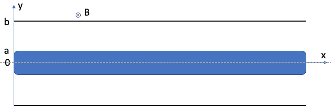
Figure 2: Simulation setup for the Diocotron instability. The 2D domain is periodic in $x$ and confined in $y$. An electron beam of a width $a$ is sitting in the middle of the domain. A uniform magnetic field B is pointing in the $z$ direction, perpendicular to the $x-y$ plane.

Figure 3 shows simulation results for the Diocotron instability using the CN pusher proposed here. The results in the figure demonstrate excellent agreement in the linear growth rate between theory and simulations for both a relatively small timestep ($\omega_{ce}\Delta t=0.45$, which is comparable to that used in Ref. [9]) and a very large one ($\omega_{ce}\Delta t=18$). Agreement is also excellent in the nonlinear stage of the simulation. Proof of charge conservation (to numerical round off) and energy conservation (to nonlinear tolerance) is also provided (panels b and d). Momentum is not exactly conserved in either simulation, but errors are much smaller with the AP integrator than the well resolved one (panel c). The growth rate of the fundamental mode is $\gamma=0.2\omega_{0}=0.01\omega_{ce}=0.045\omega_{pe}$ [9], where $\omega_{0}=d(E/B)/dy$ is the characteristic timescale of the shear in the $\mathbf{E}\times\mathbf{B}$ drift velocity. Therefore, the largest timestep considered is $\Delta t\gamma=0.18$, which is still reasonable for a second-order method. The total number of nonlinear iterations per time step increases only by a factor of 2 (from 5 to 10) when increasing $\Delta t$ by a factor of 40 for a nonlinear tolerance of $10^{-10}$, resulting in an overall CPU speedup of about 14.5.

Figure 3: Simulation results for the Diocotron instability problem. Panel a depicts the growth in amplitude of the fundamental mode ($k=2\pi/L_{x}$). Panels b, c, d are time histories of the root-mean-square (rms) of the charge continuity equation (defined as root-mean-square of the residual of Eq. 35) , the total momentum error (defined as sum of all particles momentum in the $x$-direction) and total energy error (defined as $(TE^{n+1}-TE^{n})/TE^{n}$), respectively.

4.2 Modified two-stream instability

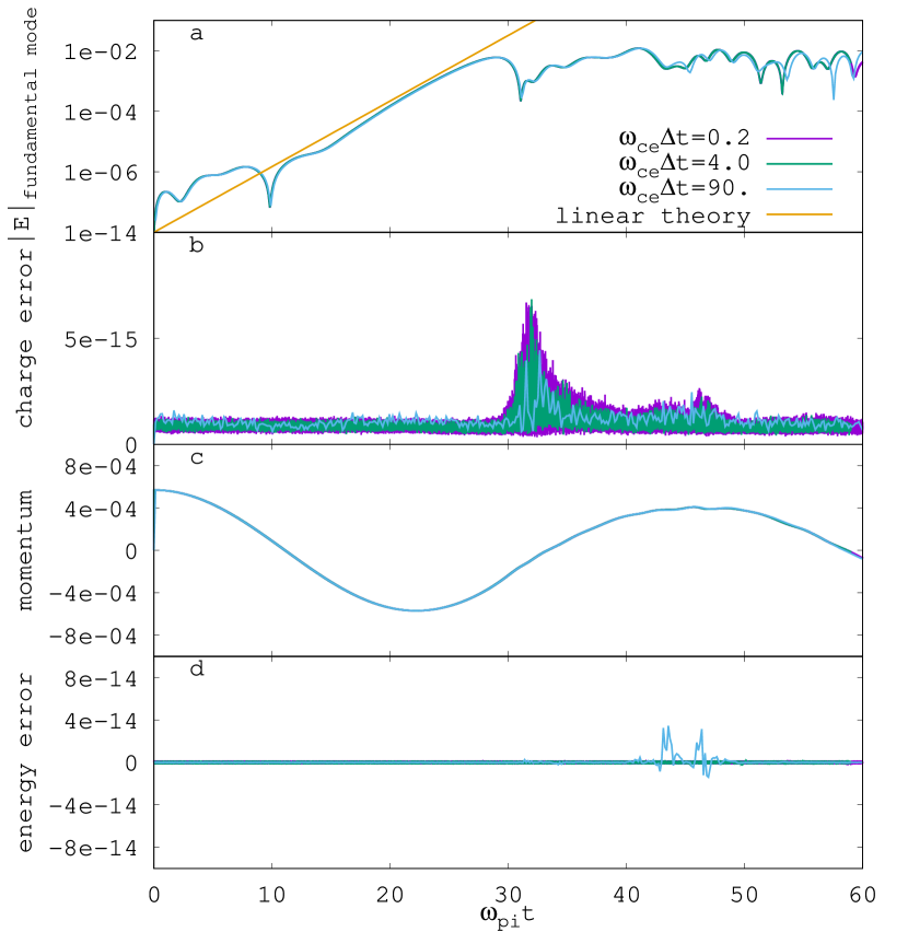
Figure 4: Simulation results for the modified two-stream instability problem. Panel a depicts the growth in the electric-field energy with three different timesteps. Panels b, c, d depict time histories of the root-mean-square (rms) of the charge continuity equation, the total momentum (normalized by $\sum_{p}m_{i}U$) , and total energy error, respectively (measured as in Fig. 3). Nonlinear tolerance is set at $10^{-10}$.

Figure 4 shows results from a simulation of the modified two-stream instability (MTSI) [30], in which electrons and ions are drifting towards each other across an external magnetic field. The MTSI happens in the regime $\omega_{ce}\gg\omega\gg\omega_{ci}$, i.e., electrons are strongly magnetized but ions are unmagnetized. The cold plasma dispersion relation is [30]:

$$1+\sin(\theta)\frac{\omega_{pe}^{2}}{\omega_{ce}^{2}}-\frac{1}{(\omega-\mathbf{k}\cdot\mathbf{U})^{2}}-\cos(\theta)\frac{\omega_{pe}^{2}}{\omega^{2}}=0,$$

where $\theta$ is a small angle between the wave vector $\mathbf{k}$ and the relative velocity $\mathbf{U}$, and the magnetic field $\mathbf{B}$ is perpendicular to $\mathbf{U}$. The simulation is performed in a 1D-3V configuration with $L_{x}=1.8229$ $\lambda_{Di}$, 32 cells and 100 particles per cell. In this test, $\omega_{ce}/\omega_{pe}=10$ and $m_{i}/m_{e}=5000$. In ion units, $m_{i}=1.0$ and $B=1/\sqrt{50}$. The magnetic field is mostly pointed in the $y$ direction but slightly tilted such that $B_{x}/B=\sin(\theta)=\sqrt{m_{e}/m_{i}}$. Electrons are stationary, and ions have a relative velocity of $U=0.5$. For these parameters, the growth rate is $\gamma=0.4992\omega_{pi}.$

We consider three timestep sizes, a small one with about 32 steps per gyroperiod ($\Delta t=0.2\omega_{ce}^{-1}$), an intermediate one with about 1.6 steps per gyro-period ($\Delta t=4.0\omega_{ce}^{-1}$), and a very large one with 0.07 steps per gyro-period ($\Delta t=90\omega_{ce}^{-1}$). The results in the figure again demonstrate excellent agreement for all timesteps, and excellent conservation of charge and energy (panels b and d).

Table 1: Solver performance for the modified two-stream instability problem with respect to mass ratio $m_{i}/m_{e}$ for the largest timestep considered. The problem is set up using ion units, so the only parameter that is varied is the electron mass. All runs employ a fixed timestep $\Delta t=0.127\omega_{pi}^{-1}$, corresponding to different timesteps in $\omega_{ce}$ units as we vary the mass ratio, as detailed in the second column of the table. The wall-clock time (WCT) for 20 timesteps, the corresponding number of nonlinear iterations (NLI) for a nonlinear tolerance of $10^{-10}$, and the estimated speedup with respect to the $\Delta t=0.2\omega_{ce}^{-1}$ case are listed. The speedup is estimated for the same final time in $\omega_{pi}$ units, assuming the cost per timestep of the $\Delta t=0.2\omega_{ce}^{-1}$ run does not fundamentally change over the span of the longer runs.

$m_{i}/m_{e}$	$\omega_{ce}\Delta t$	WCT (s)	NLI	Speedup
1000	18	5.5	5.9	40
2000	36	5.5	5.9	80
5000	90	5.18	5.9	212
10000	180	5.09	5.9	430

We look next at the performance of the solver as a function of the ion-electron mass ratio (which determines electron magnetization). Table 1 shows that both the wall-clock time and the number of nonlinear iterations stay constant as the mass ratio increases from 1000 to 10000, i.e., by a factor of 10 (with other numerical parameters unchanged), demonstrating complete insensitivity of the performance of the algorithm to the mass ratio (i.e., to the electron magnetization level) for this problem, and significant speedups as the mass ratio increases, up to 430 for the 10000 mass-ratio case.

4.3 Drift-wave instability

Finally, we consider a drift-wave instability driven by a non-uniform plasma density profile in a 2D bounded slab of magnetized plasma. The magnetic field is homogeneous and nearly perpendicular to the density gradient. The drift waves simulated are low-frequency electrostatic waves well below the ion cyclotron frequency and propagating almost perpendicularly to the magnetic field, justifying the 2D simulation. We choose a 2D simulation domain (with $L_{x}\times L_{y}=16\times 32\lambda_{De}^{2}=32\times 64\lambda_{Di}^{2}$) with a mesh of $32\times 64$ grid points. We set the $x$-direction to be periodic and the $y$-direction to be bounded with a perfect conductor. The magnetic field has a small component in the $x$-direction, i.e., $B_{x}=0.01047\ll B_{z}=0.399986$, and $B_{y}=0$. The density gradient is set to be $n(y)=\kappa L_{y}e^{-\kappa y}/(1-e^{-\kappa L_{y}})$ with $\kappa=0.14\,\lambda_{De}^{-1}=0.07\,\lambda_{Di}^{-1}$. Other parameters are $m_{e}=1/25$, $m_{i}=1$, $v_{the}=10$, $v_{thi}=1$, and $\omega_{ci}/\omega_{pi}=0.4$. These parameters are chosen identically to those used in Ref. [31] (although with a different normalization convention, as we employ ion units here). We employ 8 particles per cell and $\Delta t=0.04\,\omega_{pi}^{-1}=0.4\,\omega_{ce}^{-1}$, the same as in Ref. [31]. We will also show results with a larger timestep, $\Delta t=0.2\,\omega_{pi}^{-1}=2.0\,\omega_{ce}^{-1}$, for comparison. A sketch of the plasma density profile in the 2D domain is shown in Fig. 5.

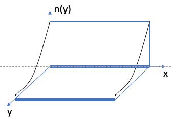
Figure 5: Density profile for the drift wave instability. The 2D domain is periodic in $x$ and confined by perfect conductors in $y$.

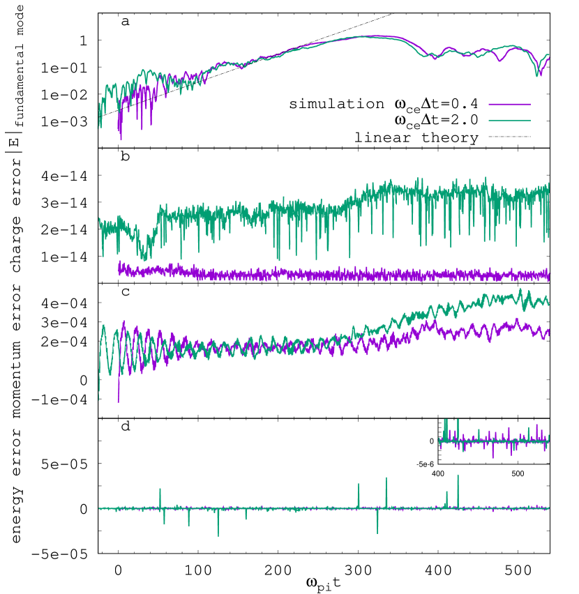
Figure 6: Simulation results for the drift-wave instability problem. Panel a depicts the growth in the electric-field energy with two different timesteps, $\Delta t=0.4\,\omega_{ce}^{-1},\,2.0\,\omega_{ce}^{-1}$. Panels b, c, d depict time histories of the root-mean-square (rms) of the charge continuity equation, the total momentum error (normalized to $\sum_{\alpha}\sum_{p}m_{p}v_{th\alpha}$), and total energy error, respectively (measured as in Fig. 3). The $\Delta t=2.0\,\omega_{ce}^{-1}$ curves are shifted left in all panels by 25 time units to provide a better comparison of the growing phase of the instability with the $\Delta t=0.4\,\omega_{ce}^{-1}$ results. The top-right corner of panel d provides additional details of the energy error over the time range [400-540].

Simulation results are shown in Fig. 6, where we find good agreement of the growth-rate of the fundamental mode with the linear theory. The growth rate is obtained as the imaginary part of the solution to the linear dispersion relation [31],

$$\sum_{\alpha}\frac{1}{T_{\alpha}}\left[1+\frac{\omega+\omega_{\alpha}^{\star}}{\sqrt{2}k_{\parallel}v_{th\alpha}}I_{0}(\hat{b}_{\alpha})e^{-\hat{b}_{\alpha}}Z\left(\frac{\omega}{\sqrt{2}k_{\parallel}v_{th\alpha}}\right)\right]=0,$$ (42)

where $\alpha$ denotes species, $v_{th\alpha}=\sqrt{T_{\alpha}/m_{\alpha}}$, $k_{\parallel}=k_{y}\cos\theta$ with $\theta$ the angle between $\mathbf{B}$ and $\mathbf{k}$, $I_{0}$ is the Bessel function of the first kind and order 0 [32], $\hat{b}_{\alpha}=r_{\alpha}^{2}(k_{x}^{2}+k_{y}^{2})$, $r_{\alpha}=v_{th\alpha}/\omega_{c\alpha}$, $\omega^{\star}=k_{y}T_{e}\kappa/m_{i}\omega_{ci}$, $\omega_{e}^{\star}=-\omega^{\star}$, $\omega_{i}^{\star}=\omega^{\star}T_{i}/T_{e}$, and $Z$ is the plasma dispersion function [33]. In this simulation, $k_{x}r_{i}=0.12$ and $k_{y}r_{i}=0.49$ for the longest wavenumber mode. The instability evolves fairly slowly. It takes a relatively long time (~250 $\omega_{pi}^{-1}$) for the mode to grow exponentially (with a growth rate of $\gamma=0.024\omega_{pi}$), and another ~50 $\omega_{pi}^{-1}$ to saturate nonlinearly. Nonlinear saturation occurs due to the flattening of the density profile. In the other panels of Fig. 6, we again see excellent charge and energy conservation, and reasonable momentum conservation. Figure 7 shows a few snapshots in time of the ion density profile. It is clear that the profile is able to maintain the initial exponential profile up to $t\sim 230\omega_{pi}^{-1}$ in the linear stage, after which the density starts to flatten out and the instability transitions into the nonlinear stage.

A few comments are in order when comparing against the results in Ref. [31]. We firstly note that the simulation algorithms are quite different. The reference reports using a guiding-center model simulated by a dipole-expansion technique with finite-size particles and explicit time-integration, while we use an asymptotic-preserving implicit PIC algorithm. Nevertheless, our simulations find good agreement with the linear theory for about as long as the simulations in the reference. Both sets of results run into a slower-growing phase before getting into the saturated nonlinear stage, which is caused by the flattening of the density gradient. While it appears that the instability gets into clear exponential growth earlier in the simulations in the reference than in ours, we speculate that this is likely due to the initialization procedure.

Another obvious difference between the two approaches is the treatment of particle boundary conditions. As is well-known, the treatment of particle boundaries in the guiding-center model can be troublesome [34], whereas in our algorithm the boundary treatment is quite natural and straightforward, as we can seamlessly transition particles to full-orbit integration if they hit the wall. In our simulations, we do this by estimating the sub-timestep according to the full-orbit time estimator described in Sec. 2.2 if a particle is reflected by the wall. We have found that this simple treatment affords both long-term accuracy and robustness in practice.

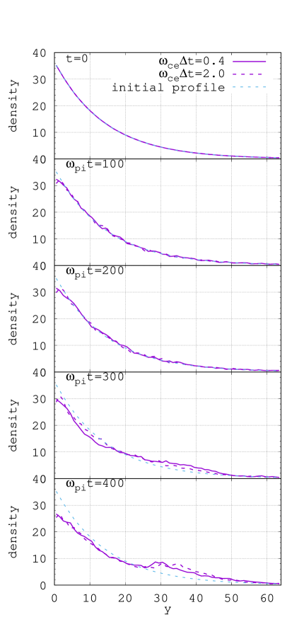
Figure 7: Ion density profiles at different times during the drift-wave instability evolution. The density is averaged over the $x$ domain. The initial density is an exponential profile. Four snapshots are depicted to show the evolution of the density profile in $y$.

There are significant differences between $\Delta t=0.4\,\omega_{ce}^{-1}$ and $\Delta t=2.0\,\omega_{ce}^{-1}$ in terms of performance. For instance, for 20 timesteps, the average number of nonlinear iterations per timestep is 4.9 and 8.1, respectively, with corresponding wall-clock times of 110 s and 182 s. We see that, as the timestep is increased by a factor of 5, the average number of Newton iterations increases only by a factor of about 1.6, and the CPU time increases proportionally, resulting in a speedup of about 3.0 to reach the same final simulation time (in $\omega_{pi}$ units). It is also worth noting that, for $\Delta t=2.0\,\omega_{ce}^{-1}$, electrons may travel on average a distance of $v_{the}\Delta t=2\lambda_{Di}$, about 14$\%$ of the gradient length scale ($1/\kappa\simeq 14\,\lambda_{Di}$). For larger timesteps, it may be necessary to include the gradient length scale in the timestep estimator, as proposed in Ref. [10].

Table 2: Solver performance with respect to mass ratio $m_{i}/m_{e}$ for the drift-wave instability problem. All runs employ a fixed timestep ${\color[rgb]{0,0,0}\,\omega_{pi}^{-1}}$, corresponding to different timesteps in $\omega_{ce}$ units as we vary the mass ratio, as detailed in the second column of the table. The wall-clock time (WCT) for 20 timesteps, the corresponding number of nonlinear iterations (NLI), and the estimated speedup with respect to the $\Delta t=0.4\,\omega_{ce}^{-1}$ case are listed.

$m_{i}/m_{e}$	$\omega_{ce}\Delta t$	WCT (s)	NLI	Speedup
25	0.4	110	4.9	1
100	1.6	113	5.3	4.8
1000	16	133	6.4	41.3
2500	40	182	8.1	60.4

It is again of interest to examine the performance of the algorithm as we increase the ion-electron mass ratio for the drift-wave problem. Table 2 shows the CPU time and nonlinear iteration count when varying the mass ratio from 25 to 2500 for $\Delta t=0.04\,\omega_{pi}^{-1}$ while keeping all other numerical parameters fixed. It shows that the wall-clock time only increases by about a factor of 1.6 as the mass ratio increases by a factor of 100, again demonstrating significant insensitivity to the electron magnetization, as expected from an AP formulation, and the potential for significant speedups as the mass ratio increases.

5 Discussion and summary

In this study, we have demonstrated an implicit, conservative PIC algorithm capable of stepping over gyration timescales in strongly magnetized regimes without apparent loss of accuracy and while conserving charge and energy exactly. The approach allows adjustment of the particle orbit timestep to the presence of boundaries, thus allowing a straightforward boundary treatment. Our implementation is for the time being electrostatic (which avoids complexities due to the presence of magnetization currents in the electromagnetic case [21]), and considers a uniform magnetic field (which avoids the $\nabla B$ drift, and allows the use of a straightforward Crank-Nicolson integrator). Even in this reduced context, the results in this study are remarkable in that they demonstrate the ability of the AP PIC algorithm to produce orders-of-magnitude computational savings in strongly magnetized environments vs. the well-resolved subcycled method, without spoiling conservation properties or long-term accuracy. Key to the development of the method is the break-up of the particle orbit into substeps in which the particle velocity is considered constant. Substeps are determined so as to resolve electric-field length scales. These substeps may traverse an arbitrary number of cells, with the local charge and energy deposition to the crossed cells computed a posteriori. If a particle hits a wall, we employ a simple second-order timestep estimator and apply a full-orbit treatment for that particle for that timestep. As a result of decoupling particle cell crossings (required for strict charge and energy conservation) from the actual orbit integration, orders of magnitude CPU speedups are realized (speedups of more than two orders of magnitude have been demonstrated for results of equivalent accuracy). It is important to note that the field solver is able to step over gyro-motion timescales (and associated Bernstein waves) without requiring the particles to resolve their gyro-motion.

Future work will consider several directions. In the short term, we will extend the CN integrator to include $\nabla B$-drift corrections (as proposed in Ref. [10]) to allow for nontrivial magnetic field configurations. In this case, the particle pushing can be done in a similar fashion as in this study, that is, a particle will be pushed in straight lines within sub-timesteps, with additional average forces and sub-timestep constraints related to the magnetic field gradient. Next, we will extend the approach to the electromagnetic regime in which the magnetic field is determined self-consistently. In this case, the effects of magnetization current need to be included. Longer-term, we will consider extending the AP orbit integrator to include finite-Larmor-radius effects. The challenge there will be to generalize the mover in Ref. [10] to the gyro-kinetic regime (for which $k\rho_{c}\sim\mathcal{O}(1)$, with $\rho_{c}$ the gyroradius and $k$ the characteristic inverse length scale), and incorporate it without losing charge and energy conservation in the implicit PIC framework.

References

- [1] G. Chen, L. Chacón, and D. C. Barnes, “An energy-and charge-conserving, implicit, electrostatic particle-in-cell algorithm,” Journal of Computational Physics, vol. 230, no. 18, pp. 7018–7036, 2011.
- [2] G. Lapenta and S. Markidis, “Particle acceleration and energy conservation in particle in cell simulations,” Physics of Plasmas, vol. 18, no. 7, p. 072101, 2011.
- [3] G. Chen and L. Chacón, “An energy-and charge-conserving, nonlinearly implicit, electromagnetic 1d-3v vlasov–darwin particle-in-cell algorithm,” Computer Physics Communications, vol. 185, no. 10, pp. 2391–2402, 2014.
- [4] G. Chen and L. Chacón, “A multi-dimensional, energy-and charge-conserving, nonlinearly implicit, electromagnetic Vlasov–Darwin particle-in-cell algorithm,” Computer Physics Communications, vol. 197, pp. 73–87, 2015.
- [5] G. Lapenta, “Exactly energy conserving semi-implicit particle in cell formulation,” Journal of Computational Physics, vol. 334, pp. 349–366, 2017.
- [6] S. Parker and C. Birdsall, “Numerical error in electron orbits with large cet,” Journal of Computational Physics, vol. 97, no. 1, pp. 91–102, 1991.
- [7] D. Barnes, T. Kamimura, J.-N. Leboeuf, and T. Tajima, “Implicit particle simulation of magnetized plasmas,” Journal of Computational Physics, vol. 52, no. 3, pp. 480–502, 1983.
- [8] H. Vu and J. Brackbill, “Accurate numerical solution of charged particle motion in a magnetic field,” Journal of Computational Physics, vol. 116, no. 2, pp. 384–387, 1995.
- [9] R. Levy and R. W. Hockney, “Computer experiments on low-density crossed-field electron beams,” The Physics of Fluids, vol. 11, no. 4, pp. 766–771, 1968.
- [10] L. F. Ricketson and L. Chacón, “An energy-conserving and asymptotic-preserving charged-particle orbit implicit time integrator for arbitrary electromagnetic fields,” Journal of Computational Physics, vol. 418, p. 109639, 2020.
- [11] F. Filbet and L. M. Rodrigues, “Asymptotically stable particle-in-cell methods for the vlasov–poisson system with a strong external magnetic field,” SIAM Journal on Numerical Analysis, vol. 54, no. 2, pp. 1120–1146, 2016.
- [12] F. Filbet and L. M. Rodrigues, “Asymptotically preserving particle-in-cell methods for inhomogeneous strongly magnetized plasmas,” SIAM Journal on Numerical Analysis, vol. 55, no. 5, pp. 2416–2443, 2017.
- [13] F. Filbet, T. Xiong, and E. Sonnendrucker, “On the vlasov–maxwell system with a strong magnetic field,” SIAM Journal on Applied Mathematics, vol. 78, no. 2, pp. 1030–1055, 2018.
- [14] F. Filbet, L. M. Rodrigues, and H. Zakerzadeh, “Convergence analysis of asymptotic preserving schemes for strongly magnetized plasmas,” Numerische Mathematik, vol. 149, no. 3, pp. 549–593, 2021.
- [15] E. Frénod, S. A. Hirstoaga, M. Lutz, and E. Sonnendrücker, “Long time behaviour of an exponential integrator for a vlasov-poisson system with strong magnetic field,” Communications in Computational Physics, vol. 18, no. 2, pp. 263–296, 2015.
- [16] N. Crouseilles, M. Lemou, F. Méhats, and X. Zhao, “Uniformly accurate particle-in-cell method for the long time solution of the two-dimensional vlasov–poisson equation with uniform strong magnetic field,” Journal of Computational Physics, vol. 346, pp. 172–190, 2017.
- [17] P. Chartier, N. Crouseilles, M. Lemou, F. Méhats, and X. Zhao, “Uniformly accurate methods for three dimensional vlasov equations under strong magnetic field with varying direction,” SIAM Journal on Scientific Computing, vol. 42, no. 2, pp. B520–B547, 2020.
- [18] S. Jin, “Efficient asymptotic-preserving (ap) schemes for some multiscale kinetic equations,” SIAM Journal on Scientific Computing, vol. 21, no. 2, pp. 441–454, 1999.
- [19] G. Chen, L. Chacon, L. Yin, B. J. Albright, D. J. Stark, and R. F. Bird, “A semi-implicit, energy-and charge-conserving particle-in-cell algorithm for the relativistic vlasov-maxwell equations,” Journal of Computational Physics, vol. 407, p. 109228, 2020.
- [20] T. H. Stix, Waves in plasmas. Springer Science & Business Media, 1992.
- [21] A. J. Brizard and C. Tronci, “Variational principles for the guiding-center vlasov-maxwell equations,” arXiv preprint arXiv:1602.05030, 2016.
- [22] R. D. Hazeltine and F. L. Waelbroeck, The framework of plasma physics. CRC Press, 2018.
- [23] O. Buneman, C. Barnes, J. Green, and D. Nielsen, “Principles and capabilities of 3-d, e-m particle simulations,” Journal of Computational Physics, vol. 38, no. 1, pp. 1–44, 1980.
- [24] O. Koshkarov, L. Chacón, G.Chen, and L. F. Ricketson, “Fast nonlinear iterative solver for an implicit, energy-conserving, asymptotic-preserving charged-particle orbit integrator,” J. Comput. Phys., 2022. accepted.
- [25] A. Stanier, L. Chacón, and G. Chen, “A fully implicit, conservative, non-linear, electromagnetic hybrid particle-ion/fluid-electron algorithm,” Journal of Computational Physics, vol. 376, pp. 597–616, 2019.
- [26] T. Z. Esirkepov, “Exact charge conservation scheme for particle-in-cell simulation with an arbitrary form-factor,” Computer Physics Communications, vol. 135, no. 2, pp. 144–153, 2001.
- [27] L. Chacón and G. Chen, “A curvilinear, fully implicit, conservative electromagnetic PIC algorithm in multiple dimensions,” Journal of Computational Physics, vol. 316, pp. 578–597, 2016.
- [28] D. G. Anderson, “Iterative procedures for nonlinear integral equations,” Journal of the ACM (JACM), vol. 12, no. 4, pp. 547–560, 1965.
- [29] H. F. Walker and P. Ni, “Anderson acceleration for fixed-point iterations,” SIAM Journal on Numerical Analysis, vol. 49, no. 4, pp. 1715–1735, 2011.
- [30] J. B. McBride, E. Ott, J. P. Boris, and J. H. Orens, “Theory and simulation of turbulent heating by the modified two-stream instability,” The Physics of Fluids, vol. 15, no. 12, pp. 2367–2383, 1972.
- [31] W. Lee and H. Okuda, “Anomalous transport and stabilization of collisionless drift-wave instabilities,” Physical Review Letters, vol. 36, no. 15, p. 870, 1976.
- [32] M. Abramowitz, I. A. Stegun, and R. H. Romer, “Handbook of mathematical functions with formulas, graphs, and mathematical tables,” 1988.
- [33] B. D. Fried and S. D. Conte, The plasma dispersion function: the Hilbert transform of the Gaussian. Academic Press, 1961.
- [34] W. Lee and H. Okuda, “A simulation model for studying low-frequency microinstabilities,” Journal of Computational Physics, vol. 26, no. 2, pp. 139–152, 1978.