Linear Regularizers Enforce the Strict Saddle Property

Linear Regularizers Enforce the Strict Saddle Property

Abstract

Satisfaction of the strict saddle property has become a standard assumption in non-convex optimization, and it ensures that many first-order optimization algorithms will almost always escape saddle points. However, functions exist in machine learning that do not satisfy this property, such as the loss function of a neural network with at least two hidden layers. First-order methods such as gradient descent may converge to non-strict saddle points of such functions, and there do not currently exist any first-order methods that reliably escape non-strict saddle points. To address this need, we demonstrate that regularizing a function with a linear term enforces the strict saddle property, and we provide justification for only regularizing locally, i.e., when the norm of the gradient falls below a certain threshold. We analyze bifurcations that may result from this form of regularization, and then we provide a selection rule for regularizers that depends only on the gradient of an objective function. This rule is shown to guarantee that gradient descent will escape the neighborhoods around a broad class of non-strict saddle points, and this behavior is demonstrated on numerical examples of non-strict saddle points common in the optimization literature.

1 Introduction

Interest in non-convex optimization has grown in recent years, driven by applications such as training deep neural networks. Often, one seeks convergence to a local minimizer in such problems because finding global minima is known to be NP complete (Murty and Kabadi 1987). To ensure convergence to minimizers, one research direction in non-convex optimization has been the identification of problem properties for which particular algorithms escape saddle points. One such property, which has become common in the non-convex optimization literature since its introduction in (Ge et al. 2015), is the strict saddle property (SSP), which states that the Hessian of every saddle point of a function has at least one negative eigenvalue. It was later shown that gradient descent and other first order methods almost always escape saddle points of objective functions that satisfy the SSP (and other mild assumptions) (Lee et al. 2016; Panageas and Piliouras 2017; Lee et al. 2017).

Because of this behavior, a growing body of non-convex optimization research has either focused on problems for which the SSP is known to hold, or simply assumed the SSP holds for a generic problem and derived convergence guarantees that result from it. However, verification of the SSP for a general, unstructured problem is difficult in practice, and there exist problems in machine learning for which the SSP does not hold, such as training a neural network with at least two hidden layers (Kawaguchi 2016).

Motivated by these challenges, we develop a linear regularization framework that will allow first-order methods to escape saddle points that are not strict. Specifically, our approach is to enforce the SSP by regularizing problems when in the vicinity of a non-strict saddle point, rather than simply assuming that the SSP holds. We show that this can be done with a linear regularizer, motivated by John Milnor’s proof that almost all choices of such a term will render a function Morse (and therefore enforce the SSP) (Milnor 1965). We are also motivated by the success of regularization techniques in convex optimization, where quadratic perturbations are used to provide strong convexity to objective functions (Facchinei and Pang 2007), and we believe that the linear regularizers we present are their natural counterparts in the non-convex setting.

1.1 Related Work

A large body of work exists on the convergence properties of gradient descent and other first-order methods on problems with the SSP, including algorithms that consider deterministic gradient descent (Dixit and Bajwa 2020; Schaeffer and McCalla 2019), and those that incorporate noise into their updates (Xu, Jin, and Yang 2017; Daneshmand et al. 2018; Yang, Hu, and Li 2017; Ge et al. 2015). These methods are shown to escape strict saddles, but have not been shown to escape non-strict saddles, and therefore rely on the SSP.

While these methods are shown to escape strict saddles in the limit, they can get stuck near strict saddles for exponential time, which can cause numerical slowdowns (Du et al. 2017). Attempts have been made to accelerate the escape near strict saddle points (Jin et al. 2017; Agarwal et al. 2017; Jin, Netrapalli, and Jordan 2018). However, first-order methods may actually converge to non-strict saddles, and such accelerated methods do not escape.

Current research into escaping non-strict saddle points uses higher-order information and/or algorithms. Perhaps the best known is (Anandkumar and Ge 2016), which guarantees convergence to a third-order optimal critical point. That paper replaces the SSP, which is a property of the Hessian, with a condition on the third-order derivative of the objective function. Work in (Zhu, Han, and Jiang 2020) expands on these results and includes simulations for a function that does not satisfy the SSP. Later work in (Chen and Toint 2021) provides a method to converge to $p^{th}$-order critical points using $p^{th}$-order information, while also demonstrating that doing so is NP-hard for $p\geq 4$. Recent work in (Truong 2021) examines the behavior of a second-order method on common examples of non-strict saddle points, and (Nguyen and Hein 2017) develop a weaker form of the SSP that guarantees escape from saddle points when training a particular neural network. In contrast, we require only first-order information and provably escape from non-strict saddles using linear regularizers under weak assumptions.

Previous research has shown that regularizing with quadratic or sums of squares (SOS) terms will make a function Morse, which is sufficient to ensure the SSP is satisfied (Lerario 2011; Nicolaescu 2011). However, no convergence or bifurcation analysis was performed on the regularized function, and indeed these results originate outside the non-convex optimization literature. We show in Example 2.6 that quadratic and SOS regularizers can actually convert a non-strict saddle point into a local minimum, and thus we do not use them.

1.2 Contributions

The contributions of this paper are the following:

• We identify certain properties that any linear regularization scheme must have, namely that regularizers cannot be chosen randomly, must be chosen locally, and must have their norms obey an upper bound dependent on $f$.

• We present a regularization scheme that has the above properties, and analyze the bifurcations it induces.

• We prove that, under a condition much weaker than the SSP, the presented regularization scheme escapes all saddle points (strict and non-strict) of $f$.

• We bound the regularization error seen at minima that is induced by linear regularizers.

The remainder of the paper is organized as follows. Section 2 establishes the theoretical motivation behind a linear regularization scheme. In Section 3, we analyze the bifurcations that may occur when regularizing, identify the properties a linear regularization scheme for SSP enforcement must have, and present a particular choice of regularizer that has these properties. In Section 4, we prove this regularization method escapes saddle points that satisfy a condition weaker than the SSP and demonstrate this escape on examples of non-strict saddle points taken from the literature. In Section 5, we analyze a hyperparameter that regulates the size of regularization and its effect on speed and accuracy, and in Section 6 we provide concluding remarks.

2 Linear Regularization

Throughout this paper, $f:\mathbb{R}^{n}\rightarrow\mathbb{R}$ denotes a function in $C^{2}$, the space of twice-continuously differentiable functions, with $L$-Lipschitz gradient $\nabla f$. The symbol $g:\mathbb{R}^{n}\rightarrow\mathbb{R}^{n}$ denotes a first-order map, with iterates generated by the sequence $x_{k}=g(x_{k-1})=g^{k}(x_{0})$. For clarity, in this paper we take $g$ to represent a gradient descent mapping, i.e., $g(x)=x-\gamma\nabla f(x)$, with $\gamma\in(0,1/L)$, though we note the results of this paper hold for any choice of $g$ that avoids strict saddle points, see (Lee et al. 2017). The following definition regards the critical points of $f$:

Definition 2.1.

1. A point $x^{*}$ is a critical point of $f$ if $\nabla f(x^{*})=0$ or, equivalently, $g(x^{*})=x^{*}$.

2. A critical point $x^{*}$ is isolated if there exists a neighborhood $U$ around $x^{*}$ with $x^{*}$ as the only critical point in $U$. Otherwise it is called non-isolated.

3. A critical point of $f$ is a local minimum if there exists a neighborhood $U$ around $x^{*}$ such that $f(x^{*})\leq f(x)$ for all $x\in U$, and a local maximum if $f(x^{*})\geq f(x)$.

4. A critical point of $f$ is a saddle point if for all neighborhoods $U$ around $x^{*}$, there exist $y,z\in U$ such that $f(y)\leq f(x^{*})\leq f(z)$.

5. A critical point of $f$ is a strict saddle if $\lambda_{min}(\nabla^{2}f(x^{*}))<0$.

6. The local stable set $W^{s}_{g}(x^{*})$ defined on some neighborhood $U$ of a critical point $x^{*}$ is the set of initial conditions of the first-order map $g$ in $U$ that converge to $x^{*}$, i.e., $W^{s}_{g}(x^{*})=\{x\in U:\lim_{k\to\infty}g^{k}(x)=x^{*}\}$. The local unstable set is defined as $W^{u}_{g}(x^{*})=\{x\in U:\lim_{k\to\infty}g^{k}(x)\neq x^{*}\}$. If $U=\mathbb{R}^{n}$, then $W^{s}_{g}(x^{*})$ ($W^{u}_{g}(x^{*})$) is the global stable (unstable) set.

Here $\lambda_{min}(\cdot)$ denotes the minimum eigenvalue of a square matrix. Lemma 2.2 states that, for almost all initial conditions, $g^{k}(x)$ does not converge to a strict saddle:

Lemma 2.2.

(Panageas and Piliouras 2017) Let $f:\mathbb{R}^{n}\rightarrow\mathbb{R}$ be a $C^{2}$ function with $L$-Lipschitz gradient. The set of initial conditions $x\in\mathbb{R}^{n}$ such that $g^{k}(x)$ converges to a strict saddle point of $f$ is of (Lebesgue) measure zero.

Proof: See Theorem 2 in (Panageas and Piliouras 2017). $\hfill\square$

The underlying principle is that, for a saddle $x^{*}$, a single negative eigenvalue of $\nabla^{2}f(x^{*})$ renders $W^{s}_{g}(x^{*})$ measure zero. This is the motivating principle behind the study of the strict saddle property:

Definition 2.3.

A function $f$ satisfies the strict saddle property (SSP) if every saddle point of $f$ is strict.

From Lemma 2.2, gradient descent will almost always avoid every strict saddle point of an objective function $f$. Therefore, if $f$ satisfies the SSP, then gradient descent will almost always avoid all saddle points of $f$. Provided gradient descent converges (i.e., $\lim_{k\to\infty}g^{k}(x)$ exists), it must then almost always converge to a local minimum. We note that $g^{k}(x)$ is guaranteed to converge in a variety of settings, including when $f$ is analytic or coercive, and we will proceed with the assumption that $f$ satisfies one of these properties.

However, verifying that a general, unstructured function satisfies the SSP is difficult in practice, and functions of interest exist that are known not to satisfy the SSP, such as the loss function of a neural network with at least two hidden layers (Kawaguchi 2016). These functions may have non-strict saddles:

Definition 2.4.

A saddle point $x^{*}$ of $f$ is a non-strict saddle if $\lambda_{min}(\nabla^{2}f(x^{*}))=0$.

We make a brief point on terminology here. The definition of a degenerate saddle varies between the dynamical systems and computer science literature, so to avoid confusion in this paper a degenerate saddle is any saddle point $x^{*}$ whose Hessian has at least one zero eigenvalue (i.e., $\nabla^{2}f(x^{*})$ is singular), while a non-strict saddle is a saddle with a Hessian whose minimum eigenvalue is zero (i.e., $\nabla^{2}f(x^{*})$ is singular and positive semi-definite). Using this terminology, any non-strict saddle is necessarily degenerate. We note that the SSP is not a non-degeneracy condition, as the Hessians of strict saddles may be degenerate, as long as they have at least one negative eigenvalue. Example 2.5 illustrates the key problem with non-strict saddle points, which is that their stable sets are not necessarily measure zero.

Example 2.5.

Consider the function $f(x,y)=\frac{1}{3}x^{3}+\frac{1}{2}y^{2}$, with negative gradient field plotted in Figure 1. Here, $(0,0)$ is a non-strict saddle of $f$, with $\nabla^{2}f(0,0)$ having $1$ and $0$ as eigenvalues. We see that $W^{s}_{g}(0,0)=\{(x,y):x>0\}$, depicted by the red region. That is, the set of initial conditions for which $g^{k}(x,y)$ converges to $(0,0)$ is not measure zero and is in fact a closed halfspace of $\mathbb{R}^{2}$.

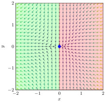
Figure 1: The negative gradient field of $f(x,y)=\frac{1}{3}x^{3}+\frac{1}{2}y^{2}$. The blue dot at $(0,0)$ denotes the non-strict saddle point, $W^{u}_{g}(0,0)$ is denoted by the green region, and $W^{s}_{g}(0,0)$ by red.

Instead of modifying gradient descent to somehow accommodate non-strict saddles, we instead wish to modify the problem itself in such a way that the modified function satisfies the SSP, either by making non-strict saddles strict or eliminating them altogether. That is, we wish to find a regularization scheme that enforces satisfaction of the SSP and thus ensures the escape of non-strict saddles. While quadratic and sums of squares regularizers are used in convex optimization, they can be harmful in non-convex problems because they can change the positive semi-definite Hessian of a non-strict saddle into a positive definite one, turning such a saddle into a local minimum:

Example 2.6.

Consider again the function $f(x,y)=\frac{1}{3}x^{3}+\frac{1}{2}y^{2}$, which has a non-strict saddle at $(0,0)$ with eigenvalues $1$ and $0$. If a sum of squares regularization term $\frac{1}{2}\alpha_{x}x^{2}+\frac{1}{2}\alpha_{y}y^{2}$ is added to $f$, then $(0,0)$ remains a critical point of the regularized function, but the eigenvalues of the regularized Hessian become $\alpha_{x}$ and $1+\alpha_{y}$, rendering $(0,0)$ a local minimum for all $\alpha_{x},\alpha_{y}>0$.

Instead, the following lemma provides motivation for using a linear regularization term.

Lemma 2.7.

(Milnor 1965) If $f:\mathbb{R}^{n}\rightarrow\mathbb{R}$ is a $C^{2}$ function, then for almost all $l\in\mathbb{R}^{n}$, the critical points of the function $f_{l}(x)=f(x)+l^{T}x$ have only non-singular Hessians.

Proof: See Lemma A in (Milnor 1965). $\hfill\square$

This lemma states that for almost any choice of $l$ (any except a set of Lebesgue measure zero) the regularized function $f_{l}$ will have only non-degenerate critical points. The fact that non-degenerate saddles are strict immediately gives us the following corollary:

Corollary 2.8.

If $f:\mathbb{R}^{n}\rightarrow\mathbb{R}$ is $C^{2}$, then for almost all $l\in\mathbb{R}^{n}$, the function $f_{l}(x)=f(x)+l^{T}x$ satisfies the SSP.

This regularization method does not affect the Hessian (i.e., $\nabla^{2}f(x)=\nabla^{2}f_{l}(x)$), avoiding the problems caused by sums of squares and quadratic regularizers. Corollary 2.8 now motivates the following question, which will be the focus of the remainder of this paper:

Question 2.9.

Can a linear regularization scheme be used to enforce the SSP on functions that do not satisfy it? If so, what properties must such a scheme have?

Though Corollary 2.8 states that almost every choice of $l$ will enforce the SSP, it is important to understand how the SSP is enforced. As we will see in the following section, this regularization method enforces satisfaction of the SSP by creating bifurcations of degenerate critical points of $f$, and we must carefully analyze these bifurcations to ensure that we attain the desired convergence properties.

3 Bifurcations

Regularization of a function perturbs non-degenerate critical points, which can be limited by a judicious choice of regularizer. However, the same is not true of degenerate critical points, as can be seen in the following example.

Example 3.1.

Consider again the function  $f(x,y)=\frac{1}{3}x^{3}+\frac{1}{2}y^{2}$ and consider two regularizations that add terms of the form $l_{x}x+l_{y}y$. The first sets $l_{x}=1$ and $l_{y}=0$ and the second sets $l_{x}=-1$ and $l_{y}=0$, and we plot the trajectory behavior of gradient descent for each in Figure 2.

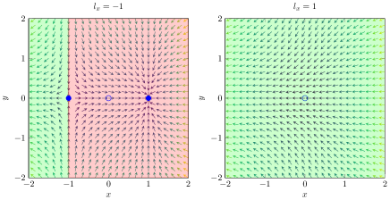
Figure 2: With $l_{x}=-1$ we create a local minimum and a strict saddle, and the escape region shifts (left). With $l_{x}=1$, the critical point is destroyed and gradient descent escapes the saddle from every initial condition (right).

Observe that when $l_{x}=-1$, the original non-strict saddle splits into a strict saddle at $(-1,0)$ and a local minimum at $(1,0)$. Both of these points are non-degenerate, satisfying the SSP as ensured by Corollary 2.8. However, we can see that $W^{s}_{g}$ (now defined for both of the resulting critical points, shown in red) has actually expanded. We have observed a local bifurcation of the non-strict saddle point at $x^{*}$.

Definition 3.2.

Let $h:\mathbb{R}^{n}\times\mathbb{R}^{k}\rightarrow\mathbb{R}$ be a $C^{2}$ function. Let $(x^{*},\mu^{*})$ be a point for which $\nabla_{x}h(x^{*},\mu^{*})=0$ and $\nabla_{x}^{2}h(x^{*},\mu^{*})$ is singular. A local bifurcation of this gradient system occurs at $x^{*}$ when a smooth change in the parameter $\mu$ away from $\mu^{*}$ induces a sudden change in the stability properties of the negative gradient vector field at $x^{*}$.

A “sudden change in stability properties” can mean a number of things, see (Guckenheimer and Holmes 2013), but in the situation presented in this paper (a codimension-one linear perturbation of a gradient system) it refers almost exclusively to saddle-node bifurcations. Example 3.1, for which $h(x,y,\mu)=\frac{1}{3}x^{3}+\frac{1}{2}y^{2}+\mu x$, illustrates a saddle-node bifurcation, where a degenerate critical point at $x^{*}$ splits into two or more critical points, or the critical point at $x^{*}$ is eliminated. This bifurcation occurs when $\mu$ crosses from zero to being positive or negative, and it results in $W^{s}_{g}(x^{*})$ changing size or dimension. Note that the saddle-node bifurcation in Example 3.1 has created a false minimum at $(1,0)$:

Definition 3.3.

A false minimum is a local minimum of $f_{l}$ that resulted from a bifurcation of a degenerate saddle point of $f$ that was caused by the linear regularizer $l^{T}x$.

In Example 3.1, one can see that for any $l_{x}<0$, a saddle-node bifurcation occurs. We also observe that when $l_{x}=1$ (and in fact whenever $l_{x}>0$) the critical point at $(0,0)$ is destroyed and all trajectories of gradient descent escape the neighborhood of $(0,0)$ (i.e., $W^{u}_{g}=\mathbb{R}^{2}$, shown in green). This gives us the following remark regarding Question 2.9:

Remark 3.4.

Any linear regularization scheme that chooses $l$ randomly has a positive probability of creating a false minimum near a non-strict saddle point of $f$.

Intuitively then, $l$ should have some dependence on $f$, and $\nabla f$ specifically is the only information available to a first-order algorithm. We note that because $l$ cannot be chosen randomly, we cannot rely solely on Corollary 2.8 to guarantee that a particular choice of $l$ enforces the SSP.

We present the following example to illustrate another property a linear regularization scheme must have.

Example 3.5.

The function $f(x)=(x-1)^{3}(x+1)^{3}$ has non-strict saddles at $x=-1$ and $x=1$. For any arbitrarily small choice of $l>0$, the non-strict saddle at $x=-1$ undergoes a saddle-node bifurcation and the non-strict saddle at $x=1$ is destroyed. For any arbitrarily small choice of $l<0$, the non-strict saddle at $x=1$ experiences a saddle-node bifurcation and the non-strict saddle at $x=-1$ is destroyed.

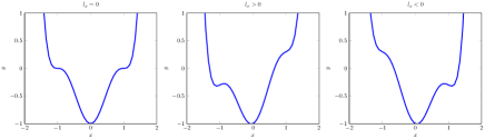
Figure 3: Plots of the function $(x-1)^{3}(x+1)^{3}+lx$ for $l=0$, $l>0$, and $l<0$. Regardless of the sign of $l$, one of the original degenerate critical points is bifurcated into a false minimum and a local maximum, and the other is eliminated for every regularizer $l\neq 0$.

A natural consequence of Example 3.5 is the following remark regarding Question 2.9:

Remark 3.6.

There exist $C^{2}$ functions for which any constant, global choice of $l\neq 0$ creates a false minimum.

Therefore, a linear regularization scheme should choose $l$ “locally”, changing the choice of $l$ when in the neighborhood of different critical points. In order to do so practically we take inspiration from (Jin et al. 2017) and define a “small gradient region”, outside of which $l=0$ and inside of which $l$ will be chosen according to some selection rule that we will devise below:

Definition 3.7.

Fix $\theta>0$ and let $L_{\theta}=\{x\in\mathbb{R}^{n}:\|\nabla f(x)\|_{2}\leq\theta\}$. That is, the small-gradient region $L_{\theta}$ is the subset of $\mathbb{R}^{n}$ for which the norm of the gradient of $f$ is less than or equal to $\theta$. For a particular $x\in L_{\theta}$, let the small-gradient neighborhood $\Theta(x)$ be the largest connected subset of $L_{\theta}$ that contains $x$.

As long as $\theta$ is chosen small enough, a point in $L_{\theta}$ must be “near” a critical point of $f$. Local linear regularization means that if an algorithm enters $L_{\theta}$ at some point $x_{0}$, then the algorithm will choose a regularizer $l$ and use it until it exits $\Theta(x_{0})$ (after which $l$ is reset to zero). Recall from Example 3.5 that a choice of $l$ that destroys one degenerate critical point may induce a saddle-node bifurcation at another. Therefore, to avoid a saddle node bifurcation within $\Theta(x_{0})$, we must ensure $\Theta(x_{0})$ contains at most one critical point or connected manifold of critical points. We formalize this idea with the following definition and assumption:

Definition 3.8.

Let $X^{*}=\{x^{*}\in\mathbb{R}^{n}:\nabla f(x^{*})=0\}$. That is, $X^{*}$ is the set of all isolated or non-isolated critical points of $f$. For a particular $x^{*}\in X^{*}$, let $\Phi(x^{*})$ be the largest connected subset of $X^{*}$ such that $x^{*}\in\Phi(x^{*})$.

If $x^{*}$ is an isolated critical point, then $\Phi(x^{*})=\{x^{*}\}$. If $x^{*}$ is non-isolated, then $\Phi(x^{*})$ is the connected critical manifold that contains $x^{*}$.

Assumption 3.9.

For $f$, there exists $\bar{\theta}>0$ such that if ${\theta<\bar{\theta}}$, then for every $x^{*}\in X^{*}$, $\Theta(x^{*})\cap X^{*}=\Phi(x^{*})$.

Note that, trivially, $X^{*}\subset L_{\theta}$ for any $\theta>0$. Assumption 3.9 simply states that $\theta$ can be chosen small enough that any critical point $x^{*}$ is isolated in $\Theta(x^{*})$ from all other critical points it is not connected to.

Recall again from Example 3.5 that a choice of $l$ that does not induce a saddle-node bifurcation at $x^{*}$ may do so for other degenerate critical points of $f$. We want to ensure that false minima, or indeed any critical points that result from a bifurcation or perturbation of a critical point other than $x^{*}$, do not end up in the set $\Theta(x^{*})$. This is guaranteed by the following theorem:

Theorem 3.10.

Let $x^{*}$ be a critical point of $f$, and let $\|l\|_{2}<\theta<\bar{\theta}$. Let $x^{*}_{l}$ be a critical point of the regularized function $f_{l}$ that resulted as a bifurcation or a perturbation of $x^{*}$. Then $x^{*}_{l}\in\Theta(x^{*})$.

Proof: See Appendix A.1. $\hfill\square$

Theorem 3.10 ensures that, even if a particular choice of $l$ induces a bifurcation at another degenerate critical point $y^{*}\in X^{*}$, the critical points that result from that bifurcation are contained within $\Theta(y^{*})$, which is disjoint from $\Theta(x^{*})$, provided $l$ is sufficiently small. In fact, Theorem 3.10 implies that the topology of $\Theta(x^{*})$ after regularization depends only on the topology of $\Theta(x^{*})$ prior to regularization. Given this fact, we now wish to choose $l$ such that, if the critical point $x^{*}$ is a degenerate saddle, regularization does not create any false minima in $\Theta(x^{*})$. We know from Remark 3.4 that the choice of $l$ for $\Theta(x^{*})$ must depend on the values of $\nabla f$ on $\Theta(x^{*})$, and from Theorem 3.10 that we must have $\|l\|_{2}\leq\theta$. Upon entering $\Theta(x^{*})$ at a point $x_{0}$, the only value of $\nabla f$ over $\Theta(x^{*})$ available is $\nabla f(x_{0})$. Therefore it is natural that the choice of $l$ for $\Theta(x^{*})$ should be some function of $\nabla f(x_{0})$. Two immediate candidates are $l=\nabla f(x_{0})$, or $l=-\nabla f(x_{0})$. To understand the implications of either of these potential choices, we look at the following theorem:

Theorem 3.11.

(Guckenheimer and Holmes 2013) Consider the function $f(x)+\mu l^{T}x$ with $\mu\in\mathbb{R}$ and $l,x\in\mathbb{R}^{n}$. Assume that for $\mu=0$ there exists a critical point $x^{*}$ such that:

1. $\nabla^{2}f(x^{*})$ has $n-1$ positive eigenvalues, and a simple eigenvalue 0 with eigenvector $v$.

2. $v^{T}l\neq 0$.

3. $v^{T}\nabla^{3}f(x^{*})(v,v)\neq 0$.

Then there is a smooth critical curve in $\mathbb{R}^{n}\times\mathbb{R}$ passing through $(x^{*},0)$ tangent to the hyperplane $\mathbb{R}^{n}\times\{0\}$ with no critical point on one side of the hyperplane and two critical points on the other side for each $\mu$. The two critical points are hyperbolic and have stable manifolds of dimensions $n-1$ and $n$ respectively.

Proof: See Theorem 3.4.1 in (Guckenheimer and Holmes 2013). $\hfill\square$

Theorem 3.11 considers a simple case: a non-strict saddle point $x^{*}$ of $f$ whose Hessian has a single zero eigenvalue and satisfies a mild third-order condition. It states that if the choice $l=u\in\mathbb{R}^{n}$ induces a saddle-node bifurcation at $x^{*}$, then the choice $l=-u$ will instead eliminate the critical point $x^{*}$. We now combine Theorem 3.11 with a concept that appears trivial at first: for some point $x_{0}$, the choice $l=-\nabla f(x_{0})$ will create a critical point of $f_{l}$ at $x_{0}$. From Theorem 3.10, this critical point at $x_{0}$ can only be the result of a bifurcation that occurred in $\Theta(x^{*})$, which contains only $x^{*}$ as a critical point. From Theorem 3.11, if the choice of $l=\nabla f(x_{0})$ induces a bifurcation of $x^{*}$, then the choice of $l=-\nabla f(x_{0})$ instead destroys the non-strict critical point.

Theorem 3.11 and the above discussion imply that the choice $l=\nabla f(x_{0})$ may be a good candidate for our regularization selection rule. Under this rule, when $g^{k}(x)$ enters the small-gradient region $L_{\theta}$ at some point $x_{0}$, $l$ is set to $\nabla f(x_{0})$ and the update law is switched to $g_{l}(x)=x-\gamma(\nabla f(x)+l)$ until $g^{k}_{l}(x)$ leaves $L_{\theta}$. Note that because linear regularization does not affect the Hessian, and by extension the Lipschitz constant $L$, $\gamma$ remains unchanged between $g$ and $g_{l}$. While this method may bear some superficial similarity to “momentum methods” such as in (Jin, Netrapalli, and Jordan 2018), this method differs in that (i) $l$ is not time-varying while in $\Theta(x^{*})$, and (ii) momentum methods rely on the SSP.

We note that Theorem 3.11 provides intuition behind this choice of regularization, but does not provide general theoretical guarantees. To do so we next determine the general cases for which locally linearly regularized gradient descent avoids non-strict saddles.

4 Exit Condition of $\Theta(x^{*})$

By construction, a point $x^{*}_{l}\in\Theta(x^{*})$ is a critical point of $f_{l}$ if and only if $\nabla f(x^{*}_{l})=-l$. Because a linear regularizer does not affect the Hessian, $\nabla^{2}f_{l}(x^{*}_{l})=\nabla^{2}f(x^{*}_{l})$. That is, if $x^{*}_{l}$ is a critical point of $f_{l}$, its convergence behavior is determined by the Hessian of $f$ at $x^{*}_{l}$. In order to analyze this, let us stratify $\Theta(x^{*})$ based on the properties of its Hessian:

Definition 4.1.

For a $C^{2}$ function $f:\mathbb{R}^{n}\rightarrow\mathbb{R}$:

• $\Lambda^{+}=\{x\in\mathbb{R}^{n}:\lambda_{min}\nabla^{2}f(x)>0\}$

• $\Lambda^{0}\,=\{x\in\mathbb{R}^{n}:\lambda_{min}\nabla^{2}f(x)=0\}$

• $\Lambda^{-}=\{x\in\mathbb{R}^{n}:\lambda_{min}\nabla^{2}f(x)<0\}$.

Note that $\mathbb{R}^{n}=\Lambda^{+}\cup\Lambda^{0}\cup\Lambda^{-}$. If $x^{*}_{l}\in\Lambda^{-}$, then it is a strict saddle, and $g^{k}(x)$ will not converge to $x^{*}_{l}$, as shown by the following lemma:

Lemma 4.2.

Let $x_{0}\in\Theta(x^{*})$ for some $x^{*}\in X^{*}$ and let $l=\nabla f(x_{0})$. Let $Y^{*}_{l}=\Theta(x^{*})\cap\Lambda^{-}\cap X^{*}_{l}$, where $X^{*}_{l}$ is the critical set of $f_{l}$. Let $\epsilon$ be drawn uniformly from the $n$-Ball with radius $\frac{\theta-\|l\|_{2}}{L}$. Then

$$\Pr\left(\lim_{k\rightarrow\infty}g_{l}^{k}(x_{0}+\epsilon)\in Y^{*}_{l}\right)=0.$$ (1)

Proof: All elements of $Y^{*}_{l}$ are strict saddle points of the function $f_{l}$. The map $g_{l}(x)$ is equivalent to gradient descent on $f_{l}$. Using this information, Corollary 9 in (Lee et al. 2016) provides the result. $\hfill\square$

Note that the one-time perturbation of $x_{0}$ is done to satisfy a genericity condition necessary to use Corollary 9 in (Lee et al. 2016), and this perturbation is only done when entering $L_{\theta}$, see (Jin et al. 2017). The restriction $\|\epsilon\|_{2}\leq\frac{\theta-\|l\|_{2}}{L}$ ensures $x_{0}+\epsilon\in\Theta(x^{*})$. Locally linearly regularized gradient descent with this perturbation is presented in Algorithm 1.

Algorithm 1 Locally Linearly Regularized Gradient Descent

  Input: Stepsize $\gamma>0$, Small gradient parameter $\theta>0$

  for k = 0,1… do

     if $\|\nabla f(x_{k})\|>\theta$ then

        $x_{k+1}\leftarrow x_{k}-\gamma\nabla f(x_{k})$

     else if $\|\nabla f(x_{k})\|\leq\theta\And\|\nabla f(x_{k-1})\|>\theta$ then

        $l\leftarrow\nabla f(x_{k})$

        $x_{k}\leftarrow x_{k}+\epsilon$ $\epsilon$ uniformly $\sim\mathbb{B}_{0}(\frac{\theta-\|l\|_{2}}{L})$

        $x_{k+1}\leftarrow x_{k}-\gamma(\nabla f(x_{k})+l)$

     else

        $x_{k+1}\leftarrow x_{k}-\gamma(\nabla f(x_{k})+l)$

     end if

  end for

If $x^{*}_{l}\notin\Lambda^{-}$, then it must lie in either $\Lambda^{0}$ or $\Lambda^{+}$. If $x^{*}_{l}\in\Lambda^{0}$, then $f_{l}$ does not satisfy the SSP. If $x^{*}_{l}\in\Lambda^{+}$ and $x^{*}$ is a saddle point, then $x^{*}_{l}$ is a false minimum by Definition 3.3. Therefore, in order to guarantee Algorithm 1 escapes $\Theta(x^{*})$ when $x^{*}$ is a saddle point, we wish to show that the choice $l=\nabla f(x_{0})$ for $x_{0}\in\Theta(x^{*})$ always results in $x^{*}_{l}\in\Lambda^{-}$, if $x^{*}_{l}$ exists. We formalize this notion with the following definition and assumption:

Definition 4.3.

Let $\Psi(\Theta(x^{*}))=\{x\in\Theta(x^{*}):\exists y\in\Theta(x^{*})\textit{ such that }\nabla f(y)=-\nabla f(x)\textit{ and }y\notin\Lambda^{-}\}$.

Assumption 4.4.

For the function $f$, for any saddle point $x^{*}$, $\Psi(\Theta(x^{*}))=\emptyset$.

If $\Psi(\Theta(x^{*}))$ is nonempty and $x_{0}\in\Psi(\Theta(x^{*}))$, then the choice $l=\nabla f(x_{0})$ creates a false minimum or degenerate point in $\Theta(x^{*})$. Assumption 4.4 therefore implies that for any saddle point $x^{*}$ of $f$ and for any point $x_{0}\in\Theta(x^{*})$, the choice $l=\nabla f(x_{0})$ will not create a false minimum or degenerate point in $\Theta(x^{*})$. This leads to the main theorem of this work, which addresses the ability of linearly regularized gradient descent to exit the small-gradient neighborhood of non-strict saddle points in finite time:

Theorem 4.5.

Let $x^{*}\in X^{*}$ be a saddle point of $f$, and let Assumptions 3.9 and 4.4 hold. Let $l=\nabla f(x_{0})$ for some $x_{0}\in\Theta(x^{*})$ with $\theta<\bar{\theta}$. Then there almost always exists a finite integer $k_{p}$ such that $g^{k_{p}}_{l}(x_{0}{\color[rgb]{1,0,0}+\epsilon})\notin\Theta(x^{*})$.

Proof: See Appendix A.2. $\hfill\square$

Theorem 4.5 states that under Assumption 4.4, Algorithm 1 exits $\Theta(x^{*})$ for any saddle point $x^{*}$ in finite time. Note Assumption 4.4 only applies to saddle points, as we do not wish to escape $\Theta(x^{*})$ if $x^{*}$ is a local minimum of $f$.

Assumption 4.4 gives a sufficient condition for which this regularization method avoids saddles. It is weaker than the SSP, allowing for a class of non-strict saddles. Identifying functions that satisfy Assumption 4.4 is therefore no harder than identifying those with the SSP, and in the following corollaries we identify two properties non-strict saddles may have that are sufficient to satisfy Assumption 4.4.

Corollary 4.6.

Let $\nabla f(\Theta(x^{*}))$ denote the set of all gradients that exist on $\Theta(x^{*})$. If $\nabla f(\Theta(x^{*}))$ lies on an open half-space of $\mathbb{R}^{n}$, then $\Psi(\Theta(x^{*}))=\emptyset$.

Trivially, if $x_{0}\in\Theta(x^{*})$, then $\nabla f(x_{0})\in\nabla f(\Theta(x^{*}))$. If $f$ satisfies the condition in Corollary 4.6, then $-\nabla f(x_{0})\notin\nabla f(\Theta(x^{*}))$. That is, for $l=\nabla f(x_{0})$ no point $x^{*}_{l}\in\Theta(x^{*})$ exists such that $\nabla f(x^{*}_{l})=-l$, which implies $f_{l}$ has no critical points in $\Theta(x^{*})$. Clearly, if $f_{l}$ has no critical points in $\Theta(x^{*})$, then Algorithm 1 exits $\Theta(x^{*})$ by Theorem 4.5. Heuristically, if a function can be approximated by an odd polynomial along at least one direction in $\Theta(x^{*})$, then by Corollary 4.6 typically $\Psi(\Theta(x^{*}))=\emptyset$, as in Example 4.7.

Example 4.7.

Consider the function $f(x,y)=\frac{1}{3}x^{3}+xy^{2}$, which has a non-strict saddle at $(0,0)$ that satisfies the condition in Corollary 4.6. This is because $\nabla_{x}f(x,y)=x^{2}+y^{2}$, which is non-negative everywhere. $W^{s}_{g}(0,0)$ is represented by the red region in Figure 4, and for every $x_{0}\in W^{s}(0,0)$, we see that the regularzer $l=\nabla f(x_{0})$ results in no critical points of $f_{l}$ in $\Theta(0,0)$, and Algorithm 1 exits $\Theta(0,0)$.

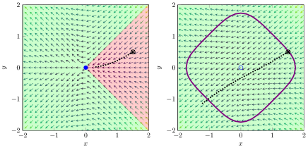
Figure 4: The point $x_{0}=(1.5,0.5)$ lies in $W^{s}_{g}(0,0)$ for the function $f(x,y)=\frac{1}{3}x^{3}+xy^{2}$, so $g^{k}(x_{0})$ converges to $(0,0)$ (left). With $l=\nabla f(x_{0})$ the critical point at $(0,0)$ is eliminated, and $g_{l}^{k}(x_{0})$ escapes $\Theta(x_{0})$ for $\theta=3$ in 7 iterations, and enters $W^{u}_{g}(0,0)$ (right).

Corollary 4.8.

If $\Lambda^{-}\cap\Theta(p)=\Theta(p)$ then $\Psi(\Theta(p))=\emptyset$.

From Theorem 4.5, if there are only strict saddles in $\Theta(x^{*})$ after regularization, then Algorithm 1 exits $\Theta(x^{*})$. Under Corollary 4.8, critical points of $f_{l}$ must be strict saddles. Generally, this condition is satisfied by objectives with non-isolated non-strict saddle points, such as in Example 4.9.

Example 4.9.

Consider the function $f(x,y)=\frac{1}{3}xy^{3}$, which has a non-strict critical subspace on the $x$-axis. For this function $-\nabla f(x,y)=\nabla f(-x,-y)$, meaning choosing $l=\nabla f(x_{0},y_{0})$ for any $(x_{0},y_{0})$ will create a critical point of $f_{l}$ at $(-x_{0},-y_{0})$. However, $\lambda_{min}(\nabla^{2}f(x,y))<0$ everywhere with $y\neq 0$, meaning $(-x_{0},-y_{0})$ will be a strict saddle, and Algorithm 1 exits $\Theta(0,0)$, shown in Figure 5.

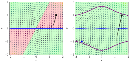
Figure 5: The function $f(x,y)=\frac{1}{3}xy^{3}$ has a critical subset on the line $y=0$. The point $x_{0}=(1.5,1)$ lies in $W^{s}_{g}$ (where $y=0$), so $g^{k}(x_{0})$ converges to $y=0$ (left). With $l=\nabla f(x_{0})$, the critical subset at $y=0$ is eliminated and a strict saddle point of $f_{l}$ is created at $(-1.5,-1)$. Then Algorithm 1 exits $\Theta(x_{0})$ for $\theta=4.7$ in 15 iterations, and enters $W^{u}_{g}$ (where $y=0$) (right).

5 The Role of the Hyperparameter $\theta$

The behavior of a locally linearly regularized algorithm is highly dependent on the hyperparameter $\theta$. Due to space constraints, determining the upper bound $\bar{\theta}$ from Assumption 3.9 for a particular function $f$ is deferred to a future publication. However, we do wish to illustrate the performance tradeoff between speed and accuracy governed by the choice of $\theta$. Intuitively, small values of $\theta$ should lead to small regularization error. This is formalized in the following theorem.

Theorem 5.1.

Assume $\theta$ is chosen small enough such that, for every critical point $x^{*}$ of $f$ that satisfies $x^{*}\in\Lambda^{+}$, we also have $\Theta(x^{*})\subset\Lambda^{+}$. If $\|l\|_{2}<\theta$, then $f_{l}$ will have exactly one critical point $x^{*}_{l}$ in $\Theta(x^{*})$, and $x^{*}_{l}$ will be a non-degenerate minimum. Additionally, if $f$ is $\alpha$-strongly convex on $\Theta(x^{*})$, then the cost error between $x^{*}_{l}$ and $x^{*}$ induced by regularizing is bounded by $f(x^{*}_{l})-f(x^{*})\leq\frac{\theta^{2}}{2\alpha}$.

Proof: See Appendix A.3. $\hfill\square$

The assumption that $f$ is $\alpha$-strongly convex in the neighborhood of local minima is standard in the SSP literature, see Assumption A3.a in (Jin et al. 2017). To examine the tradeoff between this error and runtime, we examine the Inverted Wine Bottle, the two-dimensional version of the function in Example 3.5. This function has a global minimum at $(0,0)$ surrounded by a ring of non-strict saddles on the unit circle. Unregularized gradient descent initialized outside the unit circle will become stuck and fail to reach the minimum, but locally linearly regularized gradient descent will bypass the ring and reach the origin within some regularization error. We initialize Algorithm 1 at $(1,1)$ with $\gamma=\frac{1}{54}$ and run using values of $\theta$ varying from $0.01$ to $1.7$ ($\bar{\theta}\approx 1.717$ for this function). Each run of the algorithm terminates when $\|\nabla f(x)+l\|\leq 10^{-7}$. The runtime and final cost error due to regularization are plotted in Figure 6.

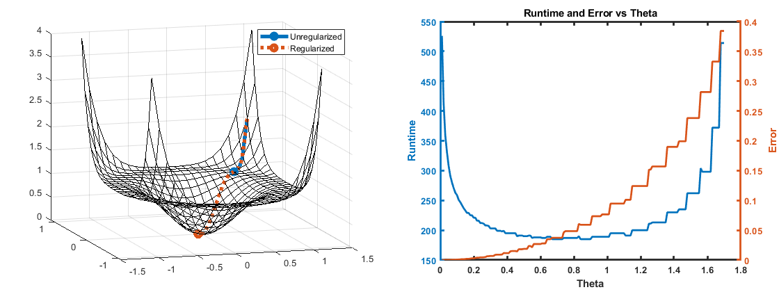
Figure 6: Left: Unregularized gradient descent (blue line) converges to the non-strict saddle ring of the inverted wine bottle $f(x,y)=1+(\sqrt{x^{2}+y^{2}}-1)^{3}(\sqrt{x^{2}+y^{2}}+1)^{3}$. Algorithm 1 with $\theta=0.7$ (orange dashed line) converges with minor error. Right: Runtime (blue) and final cost error (orange) as $\theta$ is varied. Unregularized gradient descent (not shown) had a final cost error of $1$ and a runtime of $10,979$.

Figure 6 shows that final cost error increases with $\theta$, as expected from Theorem 5.1, but the relationship between $\theta$ and the runtime is more complex. Initially, as $\theta$ is varied away from $0$, the runtime decreases. This is intuitive, as smaller choices of $\theta$ limit the use of regularizers to smaller regions of the space of iterates. However, as $\theta$ approaches $\bar{\theta}$, the runtime increases. This is due to the large perturbation of the minimum resulting from the large value of $l$. That is, for small values of $\theta$ the algorithm takes a long time to escape saddle points, and for large values of $\theta$ it takes a long time to converge to the minimum. A full analysis of how to tune $\theta$ and its effects on the performance of a locally linearly regularized algorithm is the subject of future work.

6 Concluding Remarks

We have answered Question 2.9 by demonstrating that linear regularizers can be used to enforce the SSP for non-convex objective functions, and that any such regularization scheme must both do so locally and must choose $l$ based on first-order information. We have presented a local linear regularization scheme with these properties that enforces satisfaction of the SSP. This scheme is proven to escape a broad class of isolated and non-isolated non-strict saddle points. Future work will address tuning the hyperparameter $\theta$.

Appendix A Appendix

A.1 Proof of Theorem 3.10

Consider the function $h(x,\mu)=\nabla f(x)+\mu l$ with $\|l\|_{2}<\theta$. $h$ maps $\mathbb{R}^{n}\times\mathbb{R}\rightarrow\mathbb{R}^{n}$, and $(x^{*},0)$ represents a critical point of the non-regularized function $f$. Consider a point $(x^{*}_{l},1)\in\mathbb{R}^{n}\times[0,1]$ where $\nabla f(x^{*}_{l})+l=0$, which corresponds to a critical point of the regularized function $f(x)+l^{T}x$. If the critical point of $f_{l}$ at $x^{*}_{l}$ resulted as a bifurcation originating at $x^{*}$, then the Implicit Function Theorem (Theorem 2.3 in (Matsumoto 2002)) states that there exists an open neighborhood $U\subset\mathbb{R}$ containing $\mu=1$ such that there exists a smooth function $\zeta:U\rightarrow\mathbb{R}^{n}$ such that $\zeta(1)=x^{*}_{l}$ and $\nabla f(\zeta(\mu))+\mu l=0$ for all $\mu\in U$. That is, starting at $\mu=1$ and moving in the negative direction, $(\zeta(\mu),\mu)$ is a smooth curve in $\mathbb{R}^{n}\times[0,1]$ that describes the location of a critical point for different values of $\mu$. Because $\|\nabla f(\zeta(\mu))\|_{2}=\mu\|l\|_{2}<\theta$ for all $\mu\in[0,1]$, this curve must lie in the connected subset of $L_{\theta}\times[0,1]$ that contains $(x^{*},0)$, which is $\Theta(x^{*})\times[0,1]$. Therefore $x^{*}_{l}\in\Theta(x^{*})$. $\hfill\square$

A.2 Proof of Theorem 4.5

The map $g_{l}(x)$ is equivalent to gradient descent on the function $f_{l}(x)=f(x)+l^{T}x$. Under Assumption 4.4, any critical points in $\Theta(x^{*})$ must lie in $\Lambda^{-}$, which implies they are strict saddles. Lemma 4.2 states $\lim_{k\rightarrow\infty}g_{l}^{k}(x_{0})$ is almost never a strict saddle. Therefore $\lim_{k\rightarrow\infty}g_{l}^{k}(x_{0})$ will almost always lie outside $\Theta(x^{*})$, implying it exits $\Theta(x^{*})$ in finite time. $\hfill\square$

A.3 Proof of Theorem 5.1

From Theorem 3.10, a perturbation of $x^{*}$ remains in $\Theta(x^{*})$. Because $\Lambda^{0}\cap\Theta(x^{*})=\emptyset$, no point $x\in\Theta(x^{*})$ has $\nabla^{2}f(x)$ singular, therefore there exists exactly one point $x^{*}_{l}\in\Theta(x^{*})$ for which $\nabla f(x^{*}_{l})+l=0$, and $x^{*}_{l}\in\Lambda^{+}$. $\alpha$-strong convexity on $\Theta(x^{*})$ implies that, for every point $x\in\Theta(x^{*})$, $\frac{1}{2}\|\nabla f(x)\|^{2}\geq\alpha(f(x)-f(x^{*}))$ holds. Since $x^{*}_{l}\in\Theta(x^{*})$, then $\|\nabla f(x^{*}_{l})\|_{2}\leq\theta$. The result follows by substitution. $\hfill\square$

References

- Agarwal et al. (2017) Agarwal, N.; Allen-Zhu, Z.; Bullins, B.; Hazan, E.; and Ma, T. 2017. Finding approximate local minima faster than gradient descent. In Proceedings of the 49th Annual ACM SIGACT Symposium on Theory of Computing, 1195–1199.
- Anandkumar and Ge (2016) Anandkumar, A.; and Ge, R. 2016. Efficient approaches for escaping higher order saddle points in non-convex optimization. In Conference on learning theory, 81–102. PMLR.
- Chen and Toint (2021) Chen, X.; and Toint, P. L. 2021. High-order evaluation complexity for convexly-constrained optimization with non-Lipschitzian group sparsity terms. Mathematical Programming, 187(1): 47–78.
- Daneshmand et al. (2018) Daneshmand, H.; Kohler, J.; Lucchi, A.; and Hofmann, T. 2018. Escaping saddles with stochastic gradients. In International Conference on Machine Learning, 1155–1164. PMLR.
- Dixit and Bajwa (2020) Dixit, R.; and Bajwa, W. U. 2020. Exit Time Analysis for Approximations of Gradient Descent Trajectories Around Saddle Points. arXiv preprint arXiv:2006.01106.
- Du et al. (2017) Du, S. S.; Jin, C.; Lee, J. D.; Jordan, M. I.; Poczos, B.; and Singh, A. 2017. Gradient descent can take exponential time to escape saddle points. arXiv preprint arXiv:1705.10412.
- Facchinei and Pang (2007) Facchinei, F.; and Pang, J.-S. 2007. Finite-dimensional variational inequalities and complementarity problems. Springer Science & Business Media.
- Ge et al. (2015) Ge, R.; Huang, F.; Jin, C.; and Yuan, Y. 2015. Escaping from saddle points - online stochastic gradient for tensor decomposition. In Conference on learning theory, 797–842. PMLR.