Non-asymptotic confidence bands on the probability an individual benefits from treatment (PIBT)

Abstract

The premise of this work, in a vein similar to predictive inference with quantile regression, is that observations may lie far away from their conditional expectation. In the context of causal inference, due to the missing-ness of one outcome, it is difficult to check whether an individual’s treatment effect lies close to its prediction given by the estimated Average Treatment Effect (ATE) or Conditional Average Treatment Effect (CATE). With the aim of augmenting the inference with these estimands in practice, we further study an existing distribution-free framework for the plug-in estimation of bounds on the probability an individual benefits from treatment (PIBT), a generally inestimable quantity that would concisely summarize an intervention’s efficacy if it could be known. Given the innate uncertainty in the target population-level bounds on PIBT, we seek to better understand the margin of error for the estimation of these target parameters in order to help discern whether estimated bounds on treatment efficacy are tight (or wide) due to random chance or not. In particular, we present non-asymptotic guarantees to the estimation of bounds on marginal PIBT for a randomized controlled trial (RCT) setting. We also derive new non-asymptotic results for the case where we would like to understand heterogeneity in PIBT across strata of pre-treatment covariates, with one of our main results in this setting making strategic use of regression residuals. These results, especially those in the RCT case, can be used to help with formal statistical power analyses and frequentist confidence statements for settings where we are interested in inferring PIBT through the target bounds under minimal parametric assumptions.

1 Introduction

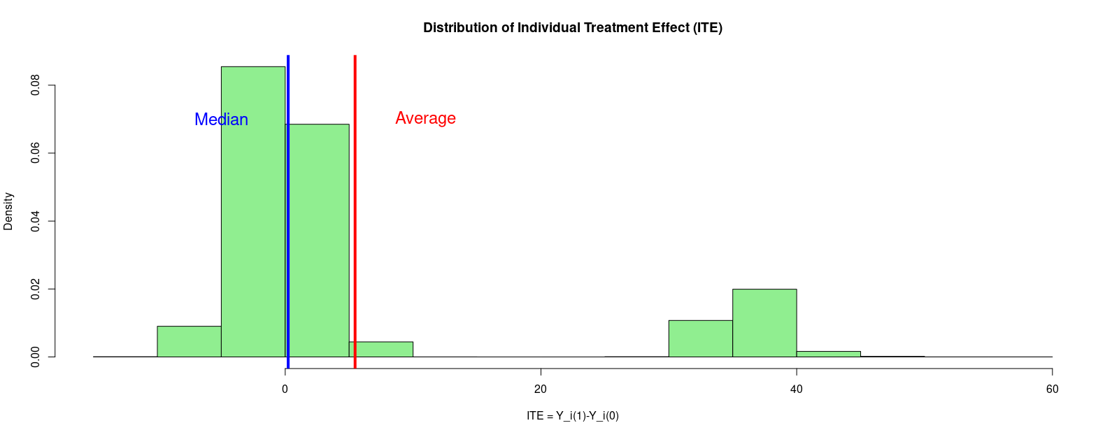
Figure 1: A hypothetical distribution for the Individual Treatment Effects. Here, the mean is positive yet the probability an individual’s treatment outcome is better (larger in value) than their control outcome is approximately 50%.

We are interested in the individual treatment effect (ITE):

$$\Delta_{i}:=Y_{i}(1)-Y_{i}(0),\ i=1,2,\dots,N,$$

where $Y_{i}(w)$ for $w=0,1$ is known as a potential outcome (Splawa-Neyman et al.,, 1990; Rubin,, 1974) and equivalently as a counterfactual (Pearl,, 2009; Hernán and Robins,, 2020). Here, $Y_{i}(w)$ corresponds to the outcome $Y_{i}$ of interest when a hypothetical experimenter intervenes with nature to force the binary exposure indicator $W_{i}$ for individual $i$ to be little $w\in\{0,1\}$, typically through random assignment in an experiment. This intervention can also be denoted by (Pearl,, 2009)’s “do” operator: $Y_{i}(w)$ is the outcome we observe under $\text{do}(W_{i}=w)$.

Suppose a large value of the observed outcome $Y_{i}=W_{i}Y_{i}(1)+[1-W_{i}]Y_{i}(0)$ is “good” for an individual. Assuming we wish to show $W_{i}=1$ is effective at accomplishing this, we will consider an individual such that

$$\Delta_{i}>\delta$$ (1)

to have benefited from treatment. We can take $\delta$ to be any relevant threshold we’d like, such as $\delta=0$. We may also reverse the inequality if more appropriate. Moreover, if the outcome of interest is strictly positive, we may alternatively define benefiting from treatment in terms of the ratio of an individual’s potential outcomes being above a threshold as we discuss in Section 2.4. For simplicity of presentation and without any loss of generality for these alternative definitions which our results can be applied to, we will work with definition given by the inequality in (1).

As can be appreciated from the hypothetical distribution of the individual treatment effects in Figure 1, it is very well possible that the average of the individual treatment effect distribution is pulled by outliers and therefore may mislead us. This example motivates our interest in the probability an individual benefits from treatment (PIBT) as provided in Definition 1.

Definition 1 (The probability an individual benefits from treatment (PIBT)).

To understand heterogeneity in treatment effect for individuals across differing strata of a pre-treatment covariate, $X_{i}$, denote

$$\theta(\delta,x):=\text{Pr}\left(\Delta_{i}>\delta|X_{i}=x\right)$$

as the conditional probability an individual benefits from treatment in pre-treatment covariate stratum $x$. To understand the effect of treatment for all individuals regardless of strata, denote

$$\theta(\delta):=\text{Pr}\left(\Delta_{i}>\delta\right)$$

as the marginal probability an individual benefits from treatment.

Here, $X_{i}$ is a pre-treatment covariate that is thought to deconfound variability in the observed outcome $Y_{i}$ that is not due to $W_{i}$ and exogenous noise alone (see Assumption 4 and Example 2) (Rubin,, 1974; Imbens and Rubin,, 2015). One can see that $\theta(\delta)=\mathbb{E}\left[\theta(X_{i},\delta)\right]$, where the expectation is taken with respect to the confounder $X_{i}$. Consider now two very similar quantities in Definition 2.

Definition 2 (Probability a treatment outcome is better than an independently drawn control outcome).

To understand heterogeneity in treatment’s effect across differing individuals and across differing strata of a pre-treatment covariate strata, denote

$$\eta(\delta,x):=\text{Pr}\left(Y_{i}(1)-Y_{j}(0)>\delta|X_{i}=X_{j}=x;i\neq j\right)$$

as the probability that a randomly selected individual in pre-treatment covariate stratum $x$ has a treatment potential outcome that is better than the control potential outcome of a differing randomly selected individual also in stratum $x$. To understand treatment’s effect across differing individuals overall, denote

$$\eta(\delta):=\text{Pr}\left(Y_{i}(1)-Y_{j}(0)>\delta;i\neq j\right)$$

as the overall probability that a randomly selected individual has a treatment outcome that is better than a differing randomly selected individual’s control outcome.

Of crucial importance, $\theta(\delta,x)$ and $\theta(\delta)$ are not in general the same as $\eta(\delta,x)$ and $\eta(\delta)$ in Definition 2 (Hand,, 1992; Greenland et al.,, 2020). This is because $Y_{i}(1)$ and $Y_{i}(0)$ are in general dependent random variables, while $Y_{i}(1)$ is independent of $Y_{j}(0)$ when $i\neq j$ under the standard Stable Unit Treatment Value Assumption (see Assumption 1). Under appropriate identifiability assumptions, such as Assumption 3 or Assumption 4 below, $\eta(\delta,x)$ and $\eta(\delta)$ can be identified because we can generally sample from the distributions $Y_{i}|W_{i}=w,X_{i}=x$ and $Y_{i}|W_{i}=w$ for $w=0,1$. It is impossible to sample from the joint distributions of $(Y_{i}(0),Y_{i}(1))$ marginally or given $X_{i}=x$, because an individual cannot be in both the treatment group and the control group simultaneously. So we cannot generally identify $\theta(\delta,x)$ nor $\theta(\delta)$. Not even if we are able to perfectly match individuals in opposite treatment groups based on pre-treatment covariates.

The goal nonetheless is to reason about $\theta(\delta,x)$ and $\theta(\delta)$ through estimated bounds on these quantities. Building from the work of Fan and Park, (2010), our focus is on deriving closed-form, non-asymptotic margin of errors on these estimated bounds for an overall confidence band on PIBT of the form: PIBT is contained between

$$[\text{estimator for lower bound on PIBT}]-\text{[margin of error for PIBT bounds]}$$ (2)

and

$$\text{[estimator for upper bound on PIBT]}+\text{[margin of error for PIBT bounds]}$$ (3)

with some target frequentist confidence level. This interpretation with respect to PIBT is motivated by that of Fay et al., (2018) for the bootstrap confidence intervals they calculate using the PIBT bound estimators of Fan and Park, (2010) in the randomized experiment setting.

1.0.1 Overview of our contributions

The contributions of the present work are as follows.

1. For the bounds on the marginal probability an individual benefits from treatment which are estimated with data from a randomized controlled trial (RCT), we derive a closed-form concentration inequality depending on only the sample size and the desired frequentist confidence level. As discussed in Section 2.3, this allows for a formal statistical power analysis, albeit conservative, but notably without the requirement of an asymptotic limiting distribution nor the specification of any unknown parameters (e.g. plausible effect sizes).

2. Making strategic use of regression residuals, we also discuss how to estimate, possibly in an observational setting, the PIBT conditional on strata of an individual’s pre-treatment co-variates. We accompany the proposed approach to study heterogeneity in PIBT with a simple but general theorem that suggests how to extend or obviate from this approach with regression residuals. For the approach with regression residuals, we provide tailored versions of the general statement that allow for a frequentist confidence interpretation simultaneously at all pre-treatment covariate strata. In Section 3.2.1, we provide an extended discussion of the application of this result to the canonical linear regression model.

The existing mathematical results we exploit include the following. Key to establishing the population-level target bounds on PIBT, we use the Makarov bounds first introduced in Makarov, (1982) and later generalized in (Frank et al.,, 1987; Williamson and Downs,, 1990). These works establish a distribution-free bound on the cumulative distribution function (CDF) on the sum (or difference or product) of two or more random variables having any unknown joint distribution and fixed marginal distributions. For the non-asymptotic concentration results (the margin of error derivations), the novel contribution of this paper, we use the Dvoretzky–Kiefer–Wolfowitz (DKW) inequality (Dvoretzky et al.,, 1956; Massart,, 1990; Naaman,, 2021). The DKW inequality gives a distribution free, non-asymptotic deviation inequality for the supremum difference at any evaluation point between a target CDF and its empirical analogue estimated with a sample of independent and identically distributed (i.i.d.) random variables.

1.1 Existing work

1.1.1 Bounding the Distribution of Individual Treatment Effects

Statistical inference on the CDF of the ITE distribution, $1-\theta(\delta)$, has been of interest before the present work. In particular, we are decidedly not unique in applying Makarov, (1982)’s bounds to study the ITE’s CDF. Fan and Park, (2010) estimate bounds on $1-\theta(\delta)$ under a randomized controlled trial (RCT) setting in which the distributions of $Y_{i}(1)$ and $Y_{i}(0)$ are each marginally identified. These authors present a straightforward plug-in estimation approach that uses the empirical marginal CDFs to estimate the lower bound and upper bound on $1-\theta(\delta)$ in practice. We make use of this same plug-in estimation approach for the RCT setting as well.

The contribution of this work, relative to the contribution of Fan and Park, (2010) in the RCT setting, is the concentration inequality for the estimated PIBT bounds. Under regularity conditions, the authors show asymptotically that the plug-in bound estimators follow either a normal distribution (centered at the target bound), or a truncated normal distribution, or a point mass. Exactly which distribution this is depends on the supremum difference between the two potential outcomes’ CDFs, which is unkown. Even if we knew that the asymptotic distribution of the estimator is Gaussian, a prospective power analysis further requires an estimator for the standard error (not provided in their work) to guarantee a target confidence level and margin of error (e.g. a maximum deviation of 0.05). This points to a strength of the main concentration result in this setting: despite the possibility that the plug-in estimator can have a non-trivial, possibly biased, sampling distribution in a finite sample, the confidence level we can have for a target margin of error depends only on sample size (see the discussion around Theorem 1 and Figure 3 for details).

Fay et al., (2018) further discuss the statistical inference technique of Fan and Park, (2010) in conjunction with the quantity $1-\eta(\delta)$ in Definition 2. They discuss how $1-\eta(\delta)$ (plus a tie correction term allowing for discrete outcomes) is related to the Wilcoxon-Mann-Whitney U test (Wilcoxon,, 1945; Mann and Whitney,, 1947), often used as a non-parametric alternative to the 2 sample t-test (Fay and Proschan,, 2010). Through extensive synthetic examples and an application to study vaccine efficacy, these authors demonstrate that $\eta$ and $\theta$ can be related, for example should certain parametric models hold. But they caution that one must remain very wary of Hand, (1992)’s paradox: $\theta(\delta)<1/2$ can be the case, i.e. treatment is ineffective for a majority of individuals, yet $\eta(\delta)>1/2$ may lead us to believe otherwise. Similarly, $\eta(\delta)<1/2$ and $\theta(\delta)>1/2$ can instead be the case. Relatedly, Greenland et al., (2020) cautions about the danger of conflating $\eta(\delta)$ with $\theta(\delta)$.

Interestingly, it has been established that the Makarov bounds for the marginal CDF of $\Delta_{i}$ studied in (Fan and Park,, 2010) are point-wise but not uniformly sharp (Firpo and Ridder,, 2010, 2019). This means that Makarov, (1982)’s bounds, evaluated at a point $\delta\in\text{support}(\Delta_{i})$, arise from a joint distribution on the support of $(Y_{i}(0),Y_{i}(1))$ which itself may not satisfy the constraint of (Makarov,, 1982) with respect to the fixed CDFs of one outcome. These authors then show how one can tighten the population-level Makarov bounds on the marginal ITE CDF evaluated at only a finite set of points $\delta_{1},\dots,\delta_{m}\in\text{support}(\Delta_{i})$ ($m\geq 2)$. While promising, we consider the estimation of these tightened bounds for $\delta_{1},\dots,\delta_{m}$ beyond the scope of this paper as it is not immediately clear that it is amenable to our analysis.

For continuous outcomes in a randomized experiment setting, Frandsen and Lefgren, (2021) works under a condition known as mutual stochastic increasing-ness of the potential outcomes $(Y_{i}(0),Y_{i}(1))$ (Lehmann,, 1966). The authors write that this condition, a more general way to define positive correlation, “means that individuals with higher potential outcomes in one treatment state draw from a more favorable–in the first order stochastic sense–conditional distribution of outcomes in the other state.” The plug-in estimation approach we use in the RCT case does not make the assumption of positive correlation: it works for any joint distribution on $(Y_{i}(0),Y_{i}(1))$ (Fan and Park,, 2010), including those with any type of negative association. Given that their numerical results suggest greater precision in the point estimates of the bounds on (one minus) PIBT compared to Fan and Park, (2010)’s approach, an interesting avenue for further extensions of the power analysis we propose here is to incorporate their estimation approach for greater precision in settings where we believe positive correlation between potential outcomes is justified.

Also in the context of a randomized experiment, Caughey et al., (2021) study PIBT under a randomization inference setup that is traditionally used to test the sharp null hypothesis that all individual treatment effects are constant (Fisher,, 1935). The authors extend this framework to test whether individual treatment effects are bounded, and they also present a strategic use of order statistics to reason about PIBT. Compared to the model-based approach we take here, which assumes the existence of a super-population the sample at hand is drawn from and for which our plug-in estimators provide inference for, their work appears to be a nice alternative under the differing assumption that randomness is solely due to random assignment of subjects to a treatment.

Of special note, the quantity $\theta(\delta)$ in Definition 1 when $0<\delta<1$ is equivalent to what is known as the “probability of necessity and sufficiency (PNS)” when $Y_{i}(0)$ and $Y_{i}(1)$ take on binary values (Pearl,, 1999; Tian and Pearl,, 2000; Pearl,, 2009). In this case, PNS and what we call “marginal PIBT” are given by the joint probability $\text{Pr}\left(Y_{i}(1)=1,Y_{i}(0)=0\right)$. As suggested by the intriguing use of prepositional logic terminology in its name, PNS informs us of an intervention’s effectiveness at achieving a strictly better outcome. Bounding and estimation approaches different from the approach taken by Fan and Park, (2010) (our focus) are provided in Pearl, (1999); Tian and Pearl, (2000). In particular, both experimental and observational data can be used to bound PNS. See also Cinelli and Pearl, (2021) for a recent, though less didactic, discussion on PNS and related quantities that inform about treatment’s efficacy.

1.1.2 PIBT conditional on pre-treatment covariates

Fan and Park, (2010) also discuss the conditional bounds for the conditional PIBT, $1-\theta(\delta,x)$, at the population-level along with a brief discussion of possible estimation approaches. The appendix of Frandsen and Lefgren, (2021) also discuss a generalization of the mutual stochastic increasing-ness assumption in order to arrive at bounds for $1-\theta(\delta,x)$. In the context of ordinal outcomes, using Makarov’s bounds to study the ITE, Lu et al., (2015) also consider the case we would like to condition on covariates. All three suggest some form of distributional regression, the semi-parametric estimation of a conditional CDF (Koenker et al.,, 2013; Chernozhukov et al.,, 2013; Kneib et al.,, 2021), but they give no formal theoretical guarantees and little discussion on how to conduct statistical inference with the bound estimators. We here fill in this gap.

Related to our use of pre-treatment covariates, Lei and Candès, (2021) develops prediction intervals for the individual treatment effect based on quantile regression (Koenker and Bassett,, 1978) with strategic calibration using conformal inference (Vovk et al.,, 2005; Shafer and Vovk,, 2008; Tibshirani et al.,, 2019). Moreover, this work is extended by Jin et al., (2021) to a case where unobserved confounding is possible. Our work here is complementary to these advances, in analogy to the inverse relation between quantiles and the CDF of a distribution. We direct the interested reader to the discussion in (Fan and Park,, 2010) on the use of Makarov’s bounds to further obtain bounds on the quantiles of the marginal distribution of the individual treatment effects. With respect to theoretical guarantees, Theorem 3 below is with respect to the supremum of any inputted pre-treatment covariate level, whereas the guarantees of Lei and Candès, (2021) are with respect to any single randomly generated covariate level. This is a subtle but important difference: one may like inference about heterogeneity in individual treatments effects to extend simultaneously to multiple individuals with fixed (non-random) covariate levels, not necessarily a single random individual. On the other hand, our work does not necessarily extend to a target population beyond that represented by our training sample, and one of the main results here (Theorem 3) makes use of a regularity condition on regression residuals that quantile regression generally avoids.

1.2 Assumptions

Throughout this work, we will assume the stable unit treatment value assumption (SUTVA) in Assumption 1.

Assumption 1 (Stable Unit Treatment Value Assumption (SUTVA)).

We quote Imbens and Rubin, (2015): “The potential outcomes for any unit do not vary with the treatments assigned to other units, and, for each unit, there are no different forms or versions of each treatment level, which lead to different potential outcomes.”

We will also assume consistency of the observed outcome throughout as given in Assumption 2.

Assumption 2 (Consistency).

The observed outcome is dictated by treatment receipt indicator $W_{i}$:

$$Y_{i}:=W_{i}Y_{i}(1)+[1-W_{i}]Y_{i}(0).$$

Depending on the setting in which we would like to bound PIBT, we will also work with differing identification assumptions which are discussed now. Assumption 3 and 4 are in line with the Neyman-Rubin potential outcome model. To demonstrate how these assumptions can come up, we provide Examples 1 and 2 which make use of Pearl, (2009)’s structural causal model (SCM).

1.2.1 The randomized controlled trial case

Assumption 3 (Strong Ignorability (Rubin,, 1974; Imbens and Rubin,, 2015)).

For $i=1,2,\dots,n$, assume $(Y_{i}(0),Y_{i}(1))\mbox{$\perp\!\!\!\perp$}W_{i}$ and $\text{Pr}\left(W_{i}=1\right)$ is bounded away from $0$ and $1$.

Example 1 next gives a situation in which the marginal independence component of Assumption 3 holds: noting that $Y_{i}(w):=h_{Y}(w,X_{i},\epsilon_{iY})$ for non-random $w=0,1$ and that $(X_{i},\epsilon_{iY})\mbox{$\perp\!\!\!\perp$}W_{i}$, it follows that $(Y_{i}(0),Y_{i}(1))$ is independent of random treatment assignment indicator $W_{i}$.

Example 1.

Let $h_{X},h_{W},$ and $h_{Y}$ be fixed functions. For $i=1,2,\dots,n$, assume the random variables of interest are generated i.i.d. according to:

$$\begin{cases}X_{i}&=h_{X}(\epsilon_{iX})\\ W_{i}&=h_{W}(\epsilon_{iW})\\ Y_{i}&=h_{Y}(W_{i},X_{i},\epsilon_{iY})\\ \end{cases}.$$

Here, $(\epsilon_{iX},\epsilon_{iW},\epsilon_{iY})$ are the latent causes for variation in $(X_{i},W_{i},Y_{i})$, and they are mutually independent.

1.2.2 The pre-treatment covariate adjusted case

Figure 2: A DAG with common cause $X_{i}$ between $W_{i}$ and $Y_{i}$.

Assumption 4 (Strong Conditional Ignorability (Rubin,, 1974; Imbens and Rubin,, 2015)).

For $i=1,2,\dots,n$, assume $(Y_{i}(0),Y_{i}(1))\mbox{$\perp\!\!\!\perp$}W_{i}|X_{i}$ and $\text{Pr}\left(W_{i}=1\middle|X_{i}\right)$ is bounded away from $0$ and $1$ almost surely.

Example 2 which goes along with Figure 2 gives an example in which the conditional independence component of Assumption 4 holds. Conditional on $X_{i}=x$, a non-random value, we have that $Y_{i}(w)=h_{Y}(w,x,\epsilon_{iY})$ for non-random $w=0,1$. From this and the fact that $\epsilon_{iY}\mbox{$\perp\!\!\!\perp$}W_{i}$, it follows that $(Y_{i}(0),Y_{i}(1))$ is independent of random $W_{i}$ conditional on $X_{i}=x$, for any value of $x$.

Example 2.

Let $h_{X},h_{W},$ and $h_{Y}$ be fixed functions. For $i=1,2,\dots,n$, assume the random variables of interest are generated i.i.d. according to:

$$\begin{cases}X_{i}&=h_{X}(\epsilon_{iX})\\ W_{i}&=h_{W}(X_{i},\epsilon_{iW})\\ Y_{i}&=h_{Y}(W_{i},X_{i},\epsilon_{iY})\\ \end{cases}.$$

Here, $(\epsilon_{iX},\epsilon_{iW},\epsilon_{iY})$ are the latent causes for variation in $(X_{i},W_{i},Y_{i})$, and they are mutually independent.

2 PIBT bounds in a randomized controlled trial

Here, we aim to estimate bounds on $\theta(\delta)=\text{Pr}\left(Y_{i}(1)-Y_{i}(0)>\delta\right)$, the marginal PIBT in Definition 1. In order for us to identify these bounds, we will work under Assumption 3. Denote Makarov, (1982)’s lower bound and upper bound on PIBT as $\theta^{L}(\delta)$ and $\theta^{U}(\delta)$, which are such that

$$\theta^{L}(\delta)\ \leq\ \theta(\delta)=\text{Pr}\left(Y_{i}(1)-Y_{i}(0)>\delta\right)\ \leq\ \theta^{U}(\delta).$$

Denote their corresponding estimators based on i.i.d. data as $\hat{\theta}^{L}(\delta)$ and $\hat{\theta}^{U}(\delta)$, respectively. Theorem 1 is the main result in this section, providing a guarantee for the accuracy of these estimators, which we now formally define.

2.1 The target bounds on PIBT and their estimators

We refer the reader to Lemma 1 in Appendix A for the formal statement of the Makarov bounds. The target parameters $\theta^{L}(\delta)$ and $\theta^{U}(\delta)$ are in terms of the potential outcomes’ marginal CDFs. Here, the marginal CDF of $Y_{i}(w)$ is:

$$F_{w}(y):=\text{Pr}\left(Y_{i}(w)\leq y\right),$$

which is identified under Assumption 3. That is, $F_{w}(y)=\text{Pr}\left(Y_{i}\leq y|W_{i}=w\right)$, the marginal CDF of the observed outcomes in treatment group $w=0,1$. Denote the empirical cumulative distribution function (eCDF) for $Y_{i}(w)$, a natural estimator for $F_{w}(y)$, as:

$$\hat{F}_{wn}(y):=\frac{1}{n_{w}}\sum_{i:\ W_{i}=w}\mathbf{1}\left\{Y_{i}\leq y\right\}\text{ for }w=0,1.$$ (4)

Here, $\mathbf{1}\left\{\cdot\right\}$ is the indicator function. Using Lemma 1 in Appendix A, the target parameters to bound $\theta(\delta)$ across any joint distribution of $(Y_{i}(0),Y_{i}(1))$ are:

$${\theta}^{L}(\delta) = -\min\left(\inf_{y}\left\{F_{1}(y+\delta/2)-F_{0}(y-\delta/2)\right\},0\right)$$

for the lower bound, while for the upper bound we have:

$${\theta}^{U}(\delta) = 1-\max\left(\sup_{y}\left\{F_{1}(y+\delta/2)-F_{0}(y-\delta/2)\right\},0\right).$$

Correspondingly, we can obtain the bound estimators by plugging in the CDF estimators as in Fan and Park, (2010):

$$\hat{\theta}^{L}(\delta):=-\min\left(\inf_{y}\left[\hat{F}_{1n}(y+\delta/2)-\hat{F}_{0n}(y-\delta/2)\right],0\right)$$

and

$$\hat{\theta}^{U}(\delta):=1-\max\left(\sup_{y}\left[\hat{F}_{1n}(y+\delta/2)-\hat{F}_{0n}(y-\delta/2)\right],0\right)$$

for the lower bound and upper bound, respectively.

2.2 The main result in the RCT setting

Given the choice of our estimators $(\hat{\theta}^{L}(\delta),\hat{\theta}^{U}(\delta))$, the question becomes how accurate they are for a given sample size $n$. Theorem 1 provides us with this understanding.

Theorem 1 (Concentration inequality for the bounds on PIBT in an RCT).

If $(Y_{1}(0),Y_{1}(1)),\dots,(Y_{n}(0),Y_{n}(1))$ are i.i.d. and Assumption 3 (strong ignorability) holds, then for any $\alpha\in(0,1)$, we have that:

$$\text{Pr}\left(\sup_{\delta}\left\{\left|\hat{\theta}^{L}(\delta)-\theta^{L}(\delta)\right|\vee\left|\hat{\theta}^{U}(\delta)-\theta^{U}(\delta)\right|\right\}\leq\left(\frac{\log(4/\alpha)}{2}\right)^{\frac{1}{2}}\left(n_{0}^{-\frac{1}{2}}+n_{1}^{-\frac{1}{2}}\right)\right)\ \geq\ 1-\alpha.$$

In Theorem 1, "$\vee$" is the maximum between the left and right arguments. Moreover, $n_{0}$ is the number of control group units, while $n_{1}$ is the number of treatment group units. The proof of Theorem 1 is contained in Appendix B.2. The core idea is to first show that the bound estimators’ joint deviation can be understood in terms of the deviation between the potential outcome’s CDFs and eCDFs uniformly across each $y\in\text{support}(Y_{i})$ and $w=0,1$. That is, we must show that it is sufficient to bound:

$$\max_{w=0,1}\sup_{y}\left|\hat{F}_{wn}(y)-F_{w}(y)\right|$$

with high probability. Conveniently, this second part of the proof to Theorem 1 is given by the DKW inequality (Dvoretzky et al.,, 1956; Massart,, 1990; Naaman,, 2021) under the mild assumption that $Y_{i}$ for each $i$ such that $W_{i}=w$ must be i.i.d..

In Remark 1, we can see the practical implication of Theorem 3. The validity of Remark 1 follows from the definition of the target parameters, $\theta^{L}(\delta)$ and $\theta^{U}(\delta)$, and the derived margin of error for their estimation. In Section 2.3, we further discuss its practical implication with respect to a statistical power analysis.

Remark 1.

Using Theorem 1, we can say that with confidence at least $(1-\alpha)\times 100\%$, the probability an individual represented by our randomized controlled trial will benefit from treatment,

$$\theta(\delta)=\text{Pr}\left(Y_{i}(1)-Y_{i}(0)>\delta\right),$$

for any threshold $\delta$ of interest, is between

$$\hat{\theta}^{L}(\delta)-\left(\frac{\log(4/\alpha)}{2}\right)^{\frac{1}{2}}\left(n_{0}^{-\frac{1}{2}}+n_{1}^{-\frac{1}{2}}\right)$$

and

$$\hat{\theta}^{U}(\delta)+\left(\frac{\log(4/\alpha)}{2}\right)^{\frac{1}{2}}\left(n_{0}^{-\frac{1}{2}}+n_{1}^{-\frac{1}{2}}\right).$$

2.3 A power analysis with Theorem 1

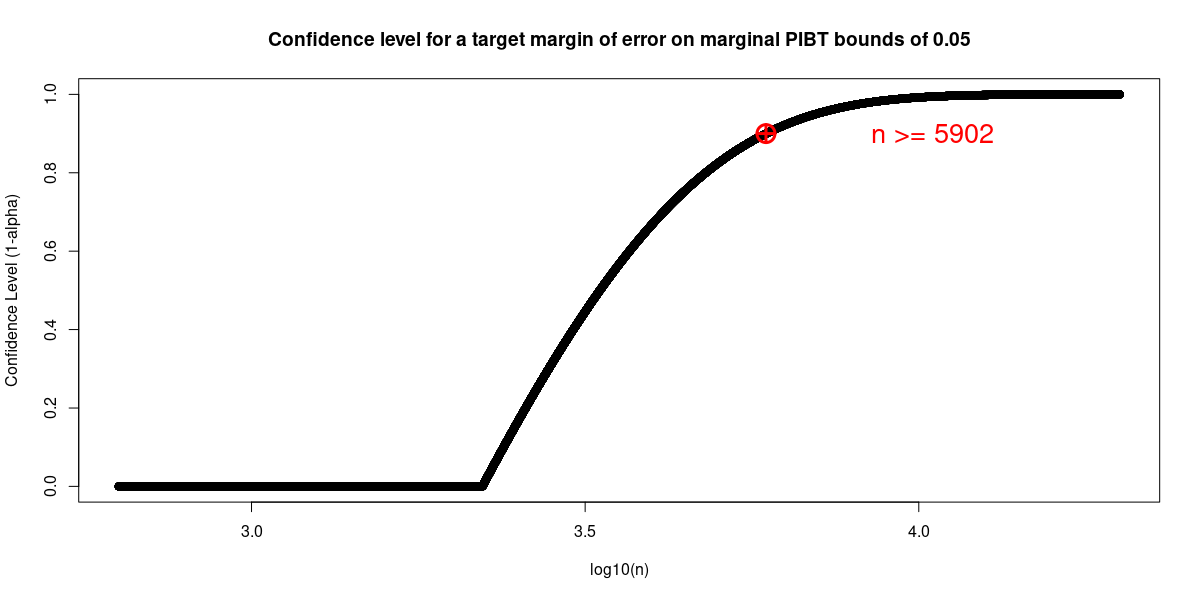
Figure 3: An example power analysis based on Theorem 1. Here, $n_{0}=n_{1}$ and $n=n_{0}+n_{1}$. The target margin of error is $0.05$, while the target confidence level is 90%. A sample size of $n\geq 5902$ guarantees this margin of error with at least a 90% confidence level.

Figure 3 presents an example power analysis making use of Theorem 1 for the case that $n_{0}=n_{1}$ and a target margin of error of $0.05$. In general, suppose our target margin of error for

$$\sup_{\delta}\left\{\left|\hat{\theta}^{L}(\delta)-\theta^{L}(\delta)\right|\vee\left|\hat{\theta}^{U}(\delta)-\theta^{U}(\delta)\right|\right\}$$

is $\varepsilon\in(0,1)$. Solving for the significance level $\alpha_{\varepsilon}$ when we set $\varepsilon$ equal to the margin of error in Theorem 1:

$$\varepsilon\ \dot{=}\ \left(\frac{\log(4/\alpha_{\varepsilon})}{2}\right)^{\frac{1}{2}}\left(n_{0}^{-\frac{1}{2}}+n_{1}^{-\frac{1}{2}}\right)$$

gives:

$$\alpha_{\varepsilon}=4\exp\left(-2\left(n_{0}^{-\frac{1}{2}}+n_{1}^{-\frac{1}{2}}\right)^{-2}\varepsilon^{2}\right).$$

The confidence level we can thus have for the target margin of error $\varepsilon$ at any given sample size $(n_{0},n_{1})$ is at least:

$$\begin{cases}1-\alpha_{\varepsilon}&\text{ if }0\leq\alpha_{\varepsilon}\leq 1\\ 0&\text{ otherwise}\end{cases}.$$

2.4 Differing definition of benefiting from treatment in terms of the ratio of potential outcomes

We also have the following simple extension to ratios of potential outcomes. It is motivated by Theorem 2 of Williamson and Downs, (1990), which derives bounds for the CDF of a sum, difference, product, or ratio of two random variables with an unknown joint distribution.

Suppose that we are interested in strictly positive potential outcomes $\tilde{Y}_{i}(0)$ and $\tilde{Y}_{i}(1)$. For example, this can be in a setting where the time to an event is the outcome of interest (Cox,, 1972; Stitelman and van der Laan,, 2010; Austin,, 2014; Schober and Vetter,, 2018; Cai and van der Laan,, 2020). Using a threshold $\tilde{\delta}>0$ (e.g. $\tilde{\delta}=1$), one may alternatively consider an individual to have benefited from treatment should the inequality

$$\tilde{Y}_{i}(1)/\tilde{Y}_{i}(0)>\tilde{\delta}$$

occur. That is, individual $i$ is deemed to have benefited from treatment should their treatment outcome be larger than their control outcome by a factor larger than $\tilde{\delta}$. Correspondingly, one may be interested in bounding the unidentifiable probability

$$\tilde{\theta}(\tilde{\delta}):=\text{Pr}\left(\tilde{Y}_{i}(1)/\tilde{Y}_{i}(0)>\tilde{\delta}\right).$$

To do so, one can work with the variable transformation

$$Y_{i}(w)\ \dot{=}\ \log(\tilde{Y}_{i}(w));w=0,1.$$

Given our definition of $\theta(\delta)$ in Definition 1 and the one-to-one nature of the log transformation, we get that

$$\tilde{\theta}(\tilde{\delta})=\theta(\delta)$$

when we set $\delta\ \dot{=}\ \log(\tilde{\delta})$. It follows that:

$$\theta^{L}(\delta)\leq\tilde{\theta}(\tilde{\delta})\leq\theta^{U}(\delta).$$

We will simply have to work with the eCDF of $\log(\tilde{Y}_{i}(w))$ when obtaining the estimators $\hat{\theta}^{L}(\delta)$ and $\hat{\theta}^{U}(\delta)$. Moreover, Theorem 1 here is still useful to conduct inference on $\tilde{\theta}(\tilde{\delta})$ under the i.i.d. assumption.

3 PIBT bounds with pre-treatment covariates

We now seek to estimate bounds on the unidentifiable probability an individual benefits from treatment (PIBT) in pre-treatment stratum $X_{i}=x$:

$$\theta(\delta,x)=\text{Pr}\left(\Delta_{i}>\delta|X_{i}=x\right).$$

Could it be known, this quantity is helpful to understand whether the benefit of receiving treatment varies across pre-treatment covariate strata. Denote the target bounds as $\theta^{L}(\delta,x)$ and $\theta^{U}(\delta,x)$, the lower and upper bound, respectively. They satisfy:

$$\theta^{L}(\delta,x)\leq\theta(\delta,x)\leq\theta^{U}(\delta,x).$$

And denote the corresponding estimators as $\hat{\theta}^{L}(\delta,x)$ and $\hat{\theta}^{U}(\delta,x)$, respectively. We would like a guarantee about how close $(\hat{\theta}^{L}(\delta,x),\hat{\theta}^{U}(\delta,x))$ is to $(\theta^{L}(\delta,x),\theta^{U}(\delta,x))$.

Remark 2 (Large enough sample at a covariate stratum?).

Importantly, we note that should a large enough sample be collected at stratum $x$ of the pre-treatment covariates, Theorem 1 can be applied for a frequentist confidence statement about $\theta(\delta,x)$ using the analogous interpretation in Remark 1. The rest of this section is useful for the case that a large enough sample is not collected for some or all of the pre-treatment covariate strata of interest.

Theorem 2 is the main non-asymptotic, non-parametric result for this setting. Theorem 3 is the adaptation of Theorem 2 to a case where we strategically use regression residuals to estimate the bounds on PIBT. For this approach with regression residuals, we show how a confidence statement about the conditional PIBT bound estimators can be written in terms of a target confidence level that is adjusted according to how accurate the regression function estimator is. In Corollary 1, we demonstrate how the statement written in this manner implies that the conditional bound estimators are as statistically efficient as the regression function estimator of choice. Moreover, Proposition 1 adopts the more general Theorem 3 to the canonical linear regression case. We demonstrate how to use this result to conduct a power analysis for the simultaneous inference on PIBT at all pre-treatment covariate strata.

3.1 The target bounds on conditional PIBT, their estimators, and the main result

The bounds $\theta^{L}(\delta,x)$ and $\theta^{U}(\delta,x)$ make use of the conditional CDFs ($w=0,1$):

$$F_{w}(y|x):=\text{Pr}\left(Y_{i}(w)\leq y\middle|X_{i}=x\right)=\text{Pr}\left(Y_{i}\leq y\middle|X_{i}=x,W_{i}=w\right),$$

with the second equality due to Assumption 4 and consistency. Explicitly, due to Lemma 1 in Appendix A, we have:

$$\theta^{L}(\delta,x)=-\min\left(\inf_{y}\left\{F_{1}(y+\delta/2|x)-F_{0}(y-\delta/2|x)\right\},0\right)$$

along with

$$\theta^{U}(\delta,x)=1-\max\left(\sup_{y}\left\{F_{1}(y+\delta/2|x)-F_{0}(y-\delta/2|x)\right\},0\right)$$

at the population-level. Denote

$$G(y,\delta,x):=F_{1}(y+\delta/2|x)-F_{0}(y-\delta/2|x),$$

and its corresponding estimator as $\hat{G}_{n}(y,\delta,x)$ based on the training sample. In practice, one may specify $\hat{G}_{n}(y,\delta,x)$ as the difference of two conditional CDF estimators as in Corollary 1 below. The plug-in estimators for the lower bound and upper bounds, respectively, will be:

$$\hat{\theta}^{L}(\delta,x)=-\min\left(\inf_{y}\left\{\hat{G}(y,\delta,x)\right\},0\right)$$ (5)

along with

$$\hat{\theta}^{U}(\delta,x)=1-\max\left(\sup_{y}\left\{\hat{G}_{n}(y,\delta,x)\right\},0\right).$$ (6)

With respect to this choice of $(\hat{\theta}^{L}(\cdot),\hat{\theta}^{U}(\cdot))$, Theorem 2 is a result under the most general conditions. Corollary 1 and Theorem 3 give further concreteness for how exactly to guarantee the premise of Theorem 2 with respect to $\hat{G}(y,\delta,x)$. The idea behind the generic statement in Theorem 2 is to encourage extensions, especially those with the possibility of being more statistically efficient, with less restricted conditions than those in Theorem 3, or with modeling assumptions that are tailored to the application at hand.

Theorem 2 (A non-parametric inequality about the conditional bound estimators’ deviation).

If Assumption 4 (strong conditional ignorability) holds, we have for all $\delta\in\mathbb{R}$ and all $x\in\text{support}(X_{i})$:

$$\left(\left|\hat{\theta}^{L}(\delta,x)-\theta^{L}(\delta,x)\right|\vee\left|\hat{\theta}^{U}(\delta,x)-\theta^{U}(\delta,x)\right|\right)\leq\sup_{y}\left|\hat{G}_{n}(y,\delta,x)-G(y,\delta,x)\right|.$$ (7)

If, additionally, $\hat{G}_{n}(y,\delta,x)$ is such that there exists a value $t_{\alpha}(\delta,x)$ such that:

$$\text{Pr}\left(\sup_{y}\left|\hat{G}_{n}(y,\delta,x)-G(y,\delta,x)\right|\leq t_{\alpha}(\delta,x)\right)\geq 1-\alpha,$$

then we have that:

$$\text{Pr}\left(\left|\hat{\theta}^{L}(\delta,x)-\theta^{L}(\delta,x)\right|\vee\left|\hat{\theta}^{U}(\delta,x)-\theta^{U}(\delta,x)\right|\leq t_{\alpha}(\delta,x)\right)\geq 1-\alpha.$$

The proof of Theorem 2 is contained in Appendix B.3. The implications of the non-parametric, deterministic inequality in (7) are interesting and perhaps a bit surprising. This inequality is stating that in a finite sample, the conditional bound estimators $(\hat{\theta}^{L}(\delta,x),\hat{\theta}^{U}(\delta,x))$ in (5) and (6) are jointly no less accurate at estimating $(\theta^{L}(\delta,x),\theta^{U}(\delta,x))$ as the choice of $\hat{G}_{n}(y,\delta,x)$ is for $G(y,\delta,x)$, whatever the choice may be.

As the second part of Theorem 2 suggests, we can turn (7) into a statement of frequentist confidence provided such a $t_{\alpha}(\delta,x)$ exists. Note that $t_{\alpha}(\delta,x)$ need not vary with $x$ or $\delta$; it can also be with respect to the concentration of $\hat{G}_{n}(y,\delta,x)$ uniformly across $x$ or across $\delta$ (or both) if more appropriate. Theorem 3 below is an example with such a uniform guarantee.

With regard to specifying $\hat{G}_{n}(y,\delta,x)$, one choice is to plug-in estimators of $F_{w}(y|x)$ for $w=0,1$ to arrive at a concentration inequality for the conditional bound estimators as Corollary 1 suggests. In doing so, provided the appropriate guarantee exists for the conditional CDF estimators, we actually get a strong guarantee for the bounds estimators $\hat{\theta}^{L}(\delta,x)$ and $\hat{\theta}^{U}(\delta,x)$ that is simultaneous across all threshold values $\delta$ used to define PIBT in Definition 1.

Corollary 1 (Conditional bound estimators’ concentration when plugging in conditional CDF estimators).

If Assumption 4 holds, and there exists estimators of $F_{0}(y|x)$ and $F_{1}(y|x)$ such that for $w=0,1$ and $\alpha\in(0,1)$ there exists a value $t_{w,\alpha}(x)$ such that:

$$\text{Pr}\left(\sup_{y}\left|\hat{F}_{wn}(y|x)-F_{w}(y|x)\right|\leq t_{w,\alpha}(x)\right)\geq 1-\alpha/2,$$

then we have that:

$$\text{Pr}\left(\sup_{\delta}\left(\left|\hat{\theta}^{L}(\delta,x)-\theta^{L}(\delta,x)\right|\vee\left|\hat{\theta}^{U}(\delta,x)-\theta^{U}(\delta,x)\right|\right)\leq\sum_{w=0,1}t_{w,\alpha}(x)\right)\geq 1-\alpha.$$

The proof of Corollary 1 is found in Appendix B.4.

3.2 More explicit conditional bounds with strategic use of regression residuals

Given that we are after confidence bands on PIBT in this paper, the question now becomes how exactly we should specify $\hat{F}_{wn}(y|x)$ in Corollary 1, while guaranteeing the closeness between $(\hat{\theta}^{L}(\delta,x),\hat{\theta}^{U}(\delta,x))$ and $(\theta^{L}(\delta,x),\theta^{U}(\delta,x))$ at some target confidence level. We explore one such choice using regression residuals for which such a high confidence guarantee is possible as summarized in Theorem 3. The motivation is that we would like something very similar to the plug-in estimator of $\text{Pr}\left(Y_{i}(w)\leq y\right)$ given in Equation (4) for the RCT case.

Assume $(X_{1},W_{1},Y_{1}(0),Y_{1}(1)),(X_{2},W_{2},Y_{2}(0),Y_{2}(1)),\dots,(X_{n},W_{n},Y_{n}(0),Y_{n}(1))$ are i.i.d. copies from a joint distribution. Denote the training data as:

$$\mathcal{T}:=\left\{(X_{i},W_{i},Y_{i})\right\}_{i=1}^{n},$$

where $Y_{i}=W_{i}Y_{i}(1)+[1-W_{i}]Y_{i}(0)$. Consider partitioning $\mathcal{T}$ into two independent splits $\mathcal{T}_{1}$ and $\mathcal{T}_{2}$. Denote the corresponding training indices as $\mathcal{I}_{1},\mathcal{I}_{2}\subseteq\{1,\dots,n\}$ for $\mathcal{T}_{1}$ and $\mathcal{T}_{2}$, respectively. Denote $S_{w}:=\{i:\ W_{i}=w\}$, the index set of individuals in the sample in treatment group $w=0,1$. Let $n_{w}:=\left|S_{w}\cap\mathcal{I}_{2}\right|$, the sample size in treatment group $w=0,1$ coming from data split $\mathcal{T}_{2}$.

Further, denote

$$\mu_{w}(x):=\mathbb{E}\left[Y_{i}(w)|X_{i}=x\right],$$

the conditional expectation of the potential outcome as a function of the pre-treatment covariates. Denote the regression estimate using $\mathcal{T}_{1}$ as $\hat{\mu}_{w}(x)$. Importantly, we will be able to reason about the counterfactual quantity $\mu_{w}(x)$ under Assumption 4, because:

$$\mu_{w}(x)=\mathbb{E}\left[Y_{i}|W_{i}=w,X_{i}=x\right],$$

the conditional expectation of the observed outcome in treatment group $w=0,1$. Now consider the population-level residuals:

$$R_{i}(w):=Y_{i}(w)-\mu_{w}(X_{i}).$$

Denote the approximation of $R_{i}(w)$ using $\hat{\mu}_{w}(\cdot)$ as

$$\hat{R}_{i}(w):=Y_{i}(w)-\hat{\mu}_{w}(X_{i}).$$

Motivated by the use of i.i.d. draws from the distribution $Y_{i}|W_{i}=w$ used to define $\hat{F}_{wn}(y)$ in Equation (4) for the marginal PIBT in a RCT setting, we would like to approximate draws from the distribution $Y_{i}|X_{i}=x,W_{i}=w$. With this in mind, we will specify:

$$\hat{F}_{wn}(y|x):=\frac{1}{n_{w}}\sum_{i\in S_{w}\cap\mathcal{I}_{2}}\mathbf{1}\left\{\hat{\mu}_{w}(x)+\hat{R}_{i}(w)\leq y\right\}.$$ (8)

Considering that the definition of $R_{i}(w)$ means that $Y_{i}(w)=\mu_{w}(x)+R_{i}(w)$ conditional on $X_{i}=x$, it seems that using $\hat{\mu}_{w}(x)+\hat{R}_{i}(w)$ will make this choice of $\hat{F}_{wn}(y|x)$ a reasonable approximation to $F_{w}(y|x)$.

Noting the liberal use of the plug-in principle en route to the choice of $(\hat{\theta}^{L}(\cdot),\hat{\theta}^{U}(\cdot))$ using the conditional CDF estimators in (8), a concern is now what the regularity conditions must be so that overall the conditional bound estimators are close to their true values. For any given value of $x$, $\hat{F}_{wn}(y|x)$ is reusing residuals for indices in the sample (split $\mathcal{I}_{2}$) corresponding to subjects that are not necessarily in stratum $x$. Implicit in this use is that the distribution of $(R_{i}(0),R_{i}(1))$ is the same across values of $x$. That is, we are using the independence assumption:

$$(R_{i}(0),R_{i}(1))\mbox{$\perp\!\!\!\perp$}X_{i}.$$

Beyond this regularity condition, we also require that the distribution of $\hat{R}_{i}(w)$ approximates well the distribution of $R_{i}(w)$, which in turn requires that $\hat{\mu}_{w}(\cdot)$ be close to $\mu_{w}(\cdot)$. This explains the correction to the confidence level in Theorem 3 with respect to how likely a deviation, in a uniform sense, is to occur between the true regression curve and the estimated regression curve based on random training data.

In Theorem 3, $\mathbf{X}\in\mathbb{R}^{|\mathcal{I}_{1}|\times p}$ is such that its rows are comprised of $X_{i}^{T}\in\mathbb{R}^{1\times p}$ for $i\in\mathcal{I}_{1}$.

Theorem 3 (Concentration Inequality for the Conditional Bounds on PIBT using regression residuals).

For the bound estimators in Equations (5) and (6), let us specify $\hat{G}(y|x)=\hat{F}_{1n}(y|x)-\hat{F}_{0n}(y|x)$ using the conditional CDF estimators of (8). Also let Assumption 4 (strong conditional ignorability) hold and assume further that the arbitrary joint distribution of $(R_{i}(0),R_{i}(1),X_{i})$ is such that

$$(R_{i}(0),R_{i}(1))\mbox{$\perp\!\!\!\perp$}X_{i}.$$

Conditional on $\mathbf{X}$, we have for any appropriate $\alpha\in(0,1)$:

$$\sup_{\delta,x}\left(\left|\hat{\theta}^{L}(\delta,x)-\theta^{L}(\delta,x)\right|\vee\left|\hat{\theta}^{U}(\delta,x)-\theta^{U}(\delta,x)\right|\right)$$

$$\leq \sum_{w=0,1}\sup_{r}\left\{\text{Pr}\left(r<R_{i}(w)\leq r+2t_{w}\middle|\mathbf{X}\right)\vee\text{Pr}\left(r-2t_{w}<R_{i}(w)\leq r\middle|\mathbf{X}\right)\right\}$$

$$+\left(\frac{\log(4/\alpha)}{2}\right)^{\frac{1}{2}}\left(n_{0}^{-\frac{1}{2}}+n_{1}^{-\frac{1}{2}}\right)$$

with probability at least

$$1-\alpha-\sum_{w=0,1}\text{Pr}\left(\sup_{x}\left|\hat{\mu}_{w}(x)-\mu_{w}(x)\right|>t_{w}\middle|\mathbf{X}\right).$$

Here, $t_{0},t_{1}\geq 0$ may depend on $\mathbf{X}$. If they do not, we may remove the conditional statements.

The proof of Theorem 3 is contained in Appendix B.5. Given Corollary 1, the task in this proof is to characterize the high probability concentration between the conditional CDF estimators of (8) and the true conditional CDFs. This involves a strategic application of the DKW inequality that is tailored to the imputed draws from the conditional potential outcome distribution, as well as incorporating the deviation between the estimated regression curves and the true regression curves.

Corollary 2 (Efficiency of Conditional Bound Estimators in Theorem 3).

Let $\mathcal{F}$ be the function class containing our regression estimator, $\hat{\mu}_{w}(\cdot)$. Assume there exists a sequence $g_{n,\mathcal{F}}$, depending on $n$ and the complexity of $\mathcal{F}$ (e.g. feature dimension, regularization parameters), such that

$$\max_{w=0,1}\sup_{x}\left|\hat{\mu}_{w}(x)-\mu_{w}(x)\right|\lesssim g_{n,\mathcal{F}}$$

with probability at least $1-\alpha$. Then:

$$\sup_{\delta,x}\left(\left|\hat{\theta}^{L}(\delta,x)-\theta^{L}(\delta,x)\right|\vee\left|\hat{\theta}^{U}(\delta,x)-\theta^{U}(\delta,x)\right|\right)\lesssim g_{n,\mathcal{F}}+\left(\frac{\log(4/\alpha)}{2}\right)^{\frac{1}{2}}\left(n_{0}^{-\frac{1}{2}}+n_{1}^{-\frac{1}{2}}\right)$$

holds with probability at least $1-2\alpha$, also.

Proof.

Denote $f_{w}(r)$ as the marginal density of $R_{i}(w)$ for $w=0,1$. The key here is that

$$\sup_{r}\left\{\text{Pr}\left(r<R_{i}(w)\leq r+2t_{w}\middle|\mathbf{X}\right)\vee\text{Pr}\left(r-2t<R_{i}(w)\leq r\middle|\mathbf{X}\right)\right\}$$

$$\leq 2t_{w}\max_{w=0,1}\sup_{r}f_{w}(r),$$

using that $\int_{a}^{b}h(u)du\leq\sup_{u}|h(u)||b-a|$ for any integrable function $h$. We also used that $R_{i}(w)\mbox{$\perp\!\!\!\perp$}\mathbf{X}$. Under the regularity condition that the density $f_{w}(r)$ is non-negative and bounded away from infinity, we set $t_{w}\ \dot{=}\ g_{n,\mathcal{F}}$ for $w=0,1$. This inequality and Theorem 3 allow us to arrive at the desired result. ∎

Corollary 2 means that, with respect to statistical efficiency, we lose nothing with the plug-in estimation approach by building on an estimator of $(\mu_{0}(\cdot),\mu_{1}(\cdot))$.

3.2.1 An example power analysis using Theorem 3 and a restricted regression setup

Theorem 2 and Theorem 3 provide generic moulds for a statement about inference with the estimated bounds $(\hat{\theta}^{L}(\cdot),\hat{\theta}^{U}(\cdot))$. Theorem 3 provides this inference simultaneously at all pre-treatment covariate strata $x$. A tall task. For illustrative purposes, we now consider a simple regression setup to give further concreteness to Theorem 2 and Theorem 3. With knowledge about how the pre-treatment covariates are distributed and the restricted regression setup in Assumption 5 below, we would like to understand the behavior of the margin of error for the bound estimators in Theorem 3. That is, we would like to conduct a statistical power analysis.

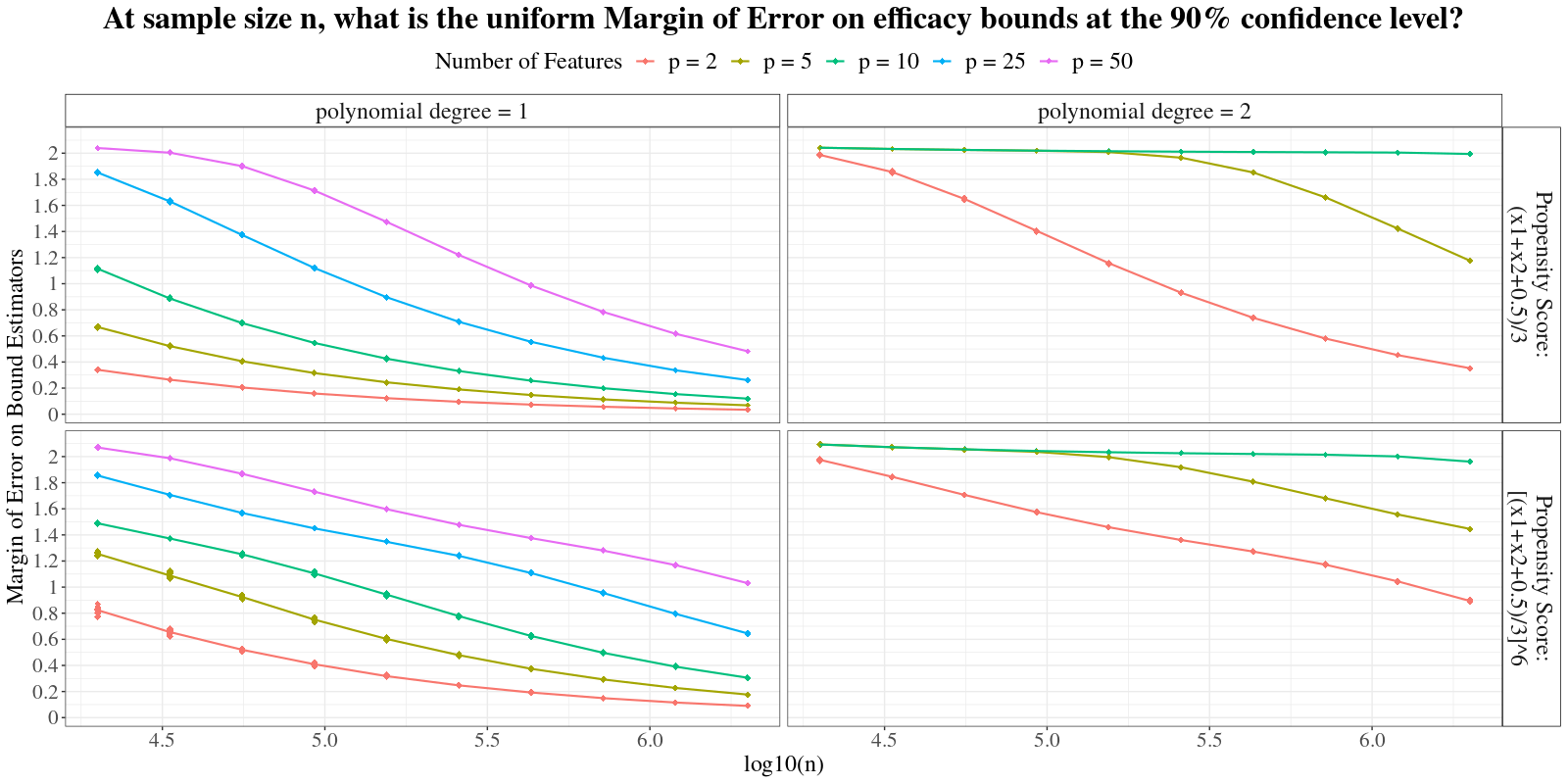
Figure 4: Power analysis based on Proposition 1. Each curve is given by the median calculated margin of error across 30 Monte Carlo simulations at the points that are also plotted. For these Monte Carlo draws, we generate $X_{ij}\stackrel{{\scriptstyle\rm i.i.d.}}{{\sim}}\text{Uniform}(0,1)$ across $i=1,\dots,n$ and $j=1,\dots,p$.

Though somewhat idealistic, the attraction of Proposition 1 below for the power analysis under Assumption 5 is that there are no unknowable parameters.

Assumption 5 (Restricted data generating mechanism).

Across $i=1,2,\dots,n$ and $w=0,1$, we will assume the i.i.d. data generating mechanism to be as follows.

1. $X_{i}$ a vector, possibly random, in $\mathbb{R}^{p}$.

2. $\mu_{w}(X_{i})=\beta_{w}^{T}\Psi_{w}(X_{i})$, where $\Psi_{w}:\mathbb{R}^{p}\to\mathbb{R}^{d}$ is a fixed mapping such that $\left\lVert\Psi_{w}(x)\right\rVert_{2}\leq 1$ and $d<n$.

3. $Y_{i}(w)=\mu_{w}(X_{i})+R_{i}(w)$.

4. $(R_{i}(0),R_{i}(1))$ have any joint distribution satisfying $(R_{i}(0),R_{i}(1))\mbox{$\perp\!\!\!\perp$}X_{i}$.

5. Marginally, $R_{i}(w)\sim\mathcal{N}(0,\sigma^{2}_{w})$.

Let ${\mathbf{\Lambda}}_{w}\in\mathbb{R}^{|\mathcal{I}_{1}\cap S_{w}|\times d}$ be such that its rows are made up by stacking $\Psi_{w}(X_{i})^{T}$ for each $i\in\mathcal{I}_{1}\cap S_{w}$. Further, let $\mathbf{Y}_{w}\in\mathbb{R}^{|\mathcal{I}_{1}\cap S_{w}|\times 1}$ contain entries for the corresponding observed outcome $Y_{i}$ for each $i\in\mathcal{I}_{1}\cap S_{w}$. In applying Theorem 3, we will estimate $\beta_{w}$ separately for $w=0,1$ using ordinary least squares regression, so that:

$$\hat{\mu}_{w}(x):=\Psi_{w}(x)^{T}\hat{\beta}_{w};\ \hat{\beta}_{w}=({\mathbf{\Lambda}}_{w}^{T}{\mathbf{\Lambda}}_{w})^{-1}{\mathbf{\Lambda}}_{w}^{T}\mathbf{Y}_{w}.$$

We note that these separate regressions are an instance of the “two-learner” meta learning of the conditional average treatment effect (CATE); CATE’s estimate with a two-learner is given by $\hat{\mu}_{1}(x)-\hat{\mu}_{0}(x)$ (Künzel et al.,, 2019). One can apply Theorem 3 with other meta-learning algorithms (Künzel et al.,, 2019; Nie and Wager,, 2020; Athey et al.,, 2019; Wager and Athey,, 2018), but Proposition 1 or similar would need to be tailored accordingly.

For Proposition 1, let $\Phi$ denote the CDF of the standard normal distribution. For a matrix $A\in\mathbb{R}^{m\times q}$, denote its operator norm as:

$${\left\lvert\kern-1.07639pt\left\lvert\kern-1.07639pt\left\lvert A\right\rvert\kern-1.07639pt\right\rvert\kern-1.07639pt\right\rvert}_{op}:=\sup_{v\in\mathbb{R}^{q}:\ \left\lVert v\right\rVert_{2}=1}\left\lVert Av\right\rVert_{2}.$$

Proposition 1 (Uniform confidence bands for the linear case with homoscedastic, Gaussian residuals).

Assume $\text{rank}({\mathbf{\Lambda}}_{w})=d$ for $w=0,1$ almost surely. Let $v_{d,\alpha}$ denote the $(1-\alpha/2)^{th}$ quantile for the $\chi^{2}_{d}$ distribution. Under Assumption 5, we have with confidence at least $(1-2\alpha)\times 100\%$ that uniformly across all pre-treatment covariate strata $x$,

$$\theta(\delta,x)=\text{Pr}\left(Y_{i}(1)-Y_{i}(0)>\delta\middle|X_{i}=x\right)$$

is contained in the interval with starting point

$$\hat{\theta}^{L}(\delta,x) -\sum_{w=0,1}\left\{\Phi\left(\sqrt{v_{d,\alpha}}{\left\lvert\kern-1.07639pt\left\lvert\kern-1.07639pt\left\lvert({\mathbf{\Lambda}}_{w}^{T}{\mathbf{\Lambda}}_{w})^{-1/2}\right\rvert\kern-1.07639pt\right\rvert\kern-1.07639pt\right\rvert}_{op}\right)-\Phi\left(-\sqrt{v_{d,\alpha}}{\left\lvert\kern-1.07639pt\left\lvert\kern-1.07639pt\left\lvert({\mathbf{\Lambda}}_{w}^{T}{\mathbf{\Lambda}}_{w})^{-1/2}\right\rvert\kern-1.07639pt\right\rvert\kern-1.07639pt\right\rvert}_{op}\right)\right\}$$

$$-\left(\frac{\log(4/\alpha)}{2}\right)^{\frac{1}{2}}\left(n_{0}^{-\frac{1}{2}}+n_{1}^{-\frac{1}{2}}\right)$$

and end point

$$\hat{\theta}^{U}(\delta,x) +\sum_{w=0,1}\left\{\Phi\left(\sqrt{v_{d,\alpha}}{\left\lvert\kern-1.07639pt\left\lvert\kern-1.07639pt\left\lvert({\mathbf{\Lambda}}_{w}^{T}{\mathbf{\Lambda}}_{w})^{-1/2}\right\rvert\kern-1.07639pt\right\rvert\kern-1.07639pt\right\rvert}_{op}\right)-\Phi\left(-\sqrt{v_{d,\alpha}}{\left\lvert\kern-1.07639pt\left\lvert\kern-1.07639pt\left\lvert({\mathbf{\Lambda}}_{w}^{T}{\mathbf{\Lambda}}_{w})^{-1/2}\right\rvert\kern-1.07639pt\right\rvert\kern-1.07639pt\right\rvert}_{op}\right)\right\}$$

$$+\left(\frac{\log(4/\alpha)}{2}\right)^{\frac{1}{2}}\left(n_{0}^{-\frac{1}{2}}+n_{1}^{-\frac{1}{2}}\right).$$

The proof of Proposition 1 is contained in Appendix B.7. The idea is to tailor Theorem 3 to the parametric assumptions and the two-learner. Moreover, the conclusion that $\theta(\delta,x)$ is contained in the specified interval follows because $\theta^{L}(\delta,x)\leq\theta(\delta,x)\leq\theta^{U}(\delta,x)$ by definition, and because the quantity added/subtracted to the estimated bounds is the form taken on by their margin of error at the $1-2\alpha$ confidence level.

Under Assumption 5, Figure 4 illustrates the behavior of the margin of error for

$$\sup_{\delta,x}\left(\left|\hat{\theta}^{L}(\delta,x)-\theta^{L}(\delta,x)\right|\vee\left|\hat{\theta}^{U}(\delta,x)-\theta^{U}(\delta,x)\right|\right)$$

at the 90% confidence level. As one can imagine, the distribution of $X_{i}$, the transformation $\Psi_{w}$ in Assumption 5, and the propensity score matter for an application of Proposition 1. That is, there may very well exist cases where the operator norm of $({\mathbf{\Lambda}}_{w}^{T}{\mathbf{\Lambda}}_{w})^{-1/2}$ does not decrease with $n$, along with cases of the propensity score where this norm decreases slowly due to insufficient treated or control units in the sample. To study this, the example summarized in Figure 4 generates data as follows:

1. We sample from a population in which each $X_{ij}\stackrel{{\scriptstyle\rm i.i.d.}}{{\sim}}\text{Uniform}(0,1)$ across $i=1,2,\dots,n$ and $j=1,2,\dots,p$.

2. The degree $q=1,2$ polynomial transformation of $X_{i}$ into $\Psi_{w}(X_{i})$ includes all possible interaction terms of degree $1\leq k\leq q$, and each polynomial term is re-scaled by $1/\sqrt{d}$ so that $\left\lVert\Psi_{w}(X_{i})\right\rVert_{2}\leq 1$ as in Assumption 5.

   • For example, $\Psi_{w}(X_{i})=(X_{i1},X_{i2},X_{i1}X_{i2},X_{i1}^{2},X_{i2}^{2})/\sqrt{5}$ when $p=q=2$.

3. The propensity score is $\text{Pr}\left(W_{i}=1\middle|X_{i}\right)=\left[\frac{1}{3}(X_{i1}+X_{i2}+0.5)\right]^{m}$ for $m=1,6$.

   • The case with $m=1$ makes it so that the number of treated and control units are very close to each other in a random sample, while the case with $m=6$ will make it so that control units are typically much more represented.

4. Moreover, the sample splitting is such that half of the observations are used to estimate $(\mu_{0}(\cdot),\mu_{1}(\cdot))$, while the other half of the observations’ residuals are used to estimate $({\theta}^{L}(\cdot),\theta^{U}(\cdot))$.

We believe the example application of Proposition 1 in Figure 4 may be regarded as a microcosm of what can occur in practice while applying the estimation procedure outlined in Section 3.2 (or similar) for the bounds on $\text{Pr}\left(Y_{i}(1)-Y_{i}(0)>\delta\middle|X_{i}=x\right)$ uniformly across $x$. The primary concerns for satisfactory margins of error are the typical concerns of regression: parsimony, multicollinearity, and feature dimension. In terms of parsimony, a more complex model specification as understood by the polynomial degree in Figure 4 requires much more data for reasonable margins of error. Regarding multicollinearity, because the features $X_{i}$ are generated with independent entries, the case of polynomial degree $1$ generally has sharper decreases in margins of error compared to the more complex models where the entries in $\Psi_{w}(X_{i})$ can become correlated. In terms of feature dimension, we also generally see slower rates of decrease in the margins of error when $p$ or $d$ is larger.

4 Discussion

For the bounds on the marginal PIBT estimated with data from a randomized controlled trial (RCT), we derive a closed-form concentration inequality depending on only the sample size and the desired frequentist confidence level. We discussed how this margin of error can be used for a formal statistical power analysis in 2.3.

Making strategic use of regression residuals, we also discussed how to estimate, possibly in an observational setting, the PIBT conditional on strata of an individual’s pre-treatment co-variates. For this approach with regression residuals, we provide novel, tailored versions of a general statement that allow for a frequentist confidence interpretation simultaneously at all pre-treatment covariate strata. To provide an example application for this result, we demonstrated in Section 3.2.1 how one may use it in a linear regression setting.

Interesting extensions of the work presented here include applying the inequality in Theorem 2 to an estimation approach that is more general than that provided in Theorem 3. Alternatively, we may like to tailor a version of Theorem 3 to certain modeling assumptions that are sufficient for interesting applications, such as involving generalized linear models (McCullagh and Nelder,, 2019). With respect to Theorem 3, we think it is also worthwhile in practice to apply it to regression scenarios beyond the linear Gaussian model. For settings where comparing an individual’s two potential outcomes in a ratio (rather than a difference) can provide interesting insight, such as studies where time to an event is of interest (Cox,, 1972; Stitelman and van der Laan,, 2010; Austin,, 2014; Schober and Vetter,, 2018; Cai and van der Laan,, 2020), it seems worthwhile to extend the discussion in Section 2.4.

5 Acknowledgements

Gabriel would like to thank NSF-GRFP DGE-1650604 for financial support. He would also like to thank Qing Zhou for encouragement on this project. And he is thankful for the helpful feedback from members of the UCLA causal inference reading group during an earlier iteration of this work.

Appendix A The Makarov bounds

Lemma 1 (The Makarov Bounds as stated in Williamson and Downs, (1990)’s Theorem 2).

Uniformly across all possible, unknown joint distributions

$$(V_{1},V_{2})\sim\text{Pr}\left(V_{1}\leq v_{1},V_{2}\leq v_{2}\right)$$

having fixed marginal CDFs $F_{1}(v_{1})=\text{Pr}\left(V_{1}\leq v_{1}\right),F_{2}(v_{2})=\text{Pr}\left(V_{2}\leq v_{1}\right)$, the CDF of $V_{1}-V_{2}$ evaluated at $\delta\in\mathbb{R}$ satisfies:

$$F^{L}(\delta) \leq\ \text{Pr}\left(V_{1}-V_{2}\leq\delta\right) \leq F^{U}(\delta),$$ (9)

where

$$F^{L}(\delta) =\ \max\left(\sup_{a,b:\ a+b=\delta}\{F_{1}(a)-F_{2}(-b)\},0\right)$$

and

$$F^{U}(\delta) =\ 1+\min\left(\inf_{a,b:\ a+b=\delta}\{F_{1}(a)-F_{2}(-b)\},0\right).$$

Lemma 1 was first proved in (Makarov,, 1982) to bound the distribution of a sum of two random variables. We present this result for subtraction, which is a simple extension, as $V_{1}-V_{2}$ is technically the sum of two random variables $V_{1}$ and $(-V_{2})$. Lemma 1’s proof was later rigourized in (Frank et al.,, 1987) and (Williamson and Downs,, 1990), who also seek bounds on the distribution of other binary operations on $V_{1}$ and $V_{2}$, like their difference, product, and their ratio, under minimal distributional assumptions.

A.1 Equivalent forms of the bounds

We note that $F^{L}(\delta)$ and $F^{U}(\delta)$ in Lemma 1 can be rewritten.

1. Consider a one-to-one change of variables $(a,b)\mapsto(u+\delta/2,-u+\delta/2)$. With it, we have equivalently:

   $$F^{L}(\delta)\ =\ \max\left(\sup_{u}\{F_{1}(u+\delta/2)-F_{2}(u-\delta/2)\},0\right)$$

   along with

   $$F^{U}(\delta)\ =\ 1+\min\left(\inf_{u}\{F_{1}(u+\delta/2)-F_{2}(u-\delta/2)\},0\right).$$

   This is in line with what we have written in Section 2 and 3 of the main text.

2. Consider instead the one-to-one change of variables $(a,b)\mapsto(u,-u+\delta)$. With it, we have equivalently:

   $$F^{L}(\delta)\ =\ \max\left(\sup_{u}\{F_{1}(u)-F_{2}(u-\delta)\},0\right)$$

   along with

   $$F^{U}(\delta)\ =\ 1+\min\left(\inf_{u}\{F_{1}(u)-F_{2}(u-\delta)\},0\right).$$

   This is in line with Fan and Park, (2010)’s Lemma 2.1 and Equation (2) and (3), and it also agrees with the alternative form given in Equations (21) and (22) of Williamson and Downs, (1990).

Moreover, it is straightforward to see that:

$$1-F^{U}(\delta)\ \leq\ \text{Pr}\left(U_{1}-U_{0}>\delta\right)\ \leq\ 1-F^{L}(\delta).$$

We make use of this in the main text when bounding PIBT.

Appendix B Proofs for the main theoretical results

B.1 The key lemma

Lemma 2 (Plug-in estimation of Makarov, (1982)’s conditional bounds).

Consider jointly distributed random variables $(U_{0},U_{1},V)$. Denote:

$$\gamma^{L}(\delta,v):=-\min\left(\inf_{u}\left\{\text{Pr}\left(U_{1}\leq u+\delta/2\middle|V=v\right)-\text{Pr}\left(U_{0}\leq u-\delta/2\middle|V=v\right)\right\},0\right)$$

and

$$\gamma^{U}(\delta,v):=1-\max\left(\sup_{u}\left\{\text{Pr}\left(U_{1}\leq u+\delta/2\middle|V=v\right)-\text{Pr}\left(U_{0}\leq u-\delta/2\middle|V=v\right)\right\},0\right),$$

the Makarov, (1982); Williamson and Downs, (1990) lower and upper bounds for $\text{Pr}\left(U_{1}-U_{0}>\delta\middle|V=v\right)$. Denote

$$H(u,\delta,v):=\text{Pr}\left(U_{1}\leq u+\delta/2\middle|V=v\right)-\text{Pr}\left(U_{0}\leq u-\delta/2\middle|V=v\right).$$

Consider any estimator $\hat{H}(u,\delta,v)$ of $H(u,\delta,v)$ based on a sample

$$\{(U_{i0},V_{i}\}_{i=1}^{n_{0}}\cup\{(U_{i1},V_{i}\}_{i=1}^{n_{1}}$$

such that $(U_{i0},V_{i})$ are i.i.d. copies of $(U_{0},V)$ for $i=1,\dots,n_{0}$ and $(U_{i1},V_{i})$ are i.i.d. copies of $(U_{1},V_{1})$ for $i=1,\dots,n_{1}$. Now let

$$\hat{\gamma}^{L}(\delta,v):=-\min\left(\inf_{u}\left\{\hat{H}(u,\delta,v)\right\},0\right)$$

and

$$\hat{\gamma}^{U}(\delta,v):=1-\max\left(\sup_{u}\left\{\hat{H}(u,\delta,v)\right\},0\right).$$

We claim for every $\delta\in\mathbb{R}$ and every $v\in\text{support}(V)$ that

$$\left|\hat{\gamma}^{L}(\delta,v)-\gamma^{L}(\delta,v)\right|\vee\left|\hat{\gamma}^{U}(\delta,v)-\gamma^{U}(\delta,v)\right| \leq \sup_{u}\left|\hat{H}(u,\delta,v)-H(u,\delta,v)\right|.$$

Proof.

For any real-valued function $g(t)$, denote:

$$g^{+}(t)=\max\left(g(t),0\right)\text{ and }g^{-}(t)=-\min\left(g(t),0\right),$$

the positive and negative parts of $g(t)$, respectively. We have the following properties we will make use of

• $g(t)=g^{+}(t)-g^{-}(t)$.

• $|g(t)|=g^{+}(t)+g^{-}(t)$.

• $g^{+}(t)=\frac{|g(t)|+g(t)}{2}$.

• $g^{-}(t)=\frac{|g(t)|-g(t)}{2}$.

Below, we will use the positive and negative parts of

$$g_{\inf}(\delta,v):=\inf_{u}H(u,\delta,v)\text{ and }g_{\sup}(\delta,v):=\sup_{u}H(u,\delta,v)$$

along with

$$\hat{g}_{\inf}(\delta,v):=\inf_{u}\hat{H}(u,\delta,v)\text{ and }\hat{g}_{\sup}(\delta,v):=\sup_{u}\hat{H}(u,\delta,v).$$

Consider:

• Lower bound on $\text{Pr}\left(U_{1}-U_{0}>\delta\middle|V=v\right)$

  We are bounding the difference

  $$\left|\hat{\gamma}^{L}(\delta,v)-\gamma^{L}(\delta,v)\right|$$

  $$= \left|g_{\inf}^{-}(\delta,v)-\hat{g}_{\inf}^{-}(\delta,v)\right|$$

  $$\overset{(i)}{=} \frac{1}{2}\left|\hat{g}_{\inf}(\delta,v)-g_{\inf}(\delta,v)+\left|g_{\inf}(\delta,v)\right|-\left|\hat{g}_{\inf}(\delta,v)\right|\right|$$

  $$\overset{(ii)}{\leq} \left|\hat{g}_{\inf}(\delta,v)-g_{\inf}(\delta,v)\right|$$

  $$= \left|\inf_{u}\hat{H}(u,\delta,v)-\inf_{u}H(u,\delta,v)\right|.$$

  In (i), we used the properties of the negative part of a function introduced above, while in (ii) we used triangle inequality followed by reverse triangle inequality. Consider that

  $$\inf_{u}\hat{H}(u,\delta,v)-\inf_{u}H(u,\delta,v)$$

  $$= \inf_{u}\left[\hat{H}(u,\delta,v)-H(u,\delta,v)+H(u,\delta,v)\right]-\inf_{u}H(u,\delta,v)$$

  $$\overset{(i)}{=} \inf_{u}\left[\hat{H}(u,\delta,v)-H(u,\delta,v)\right]$$

  $$\leq \sup_{u}\left|\hat{H}(u,\delta,v)-H(u,\delta,v)\right|.$$

  Equality (i) follows from the fact that $\inf\{a+b:\ a\in A,b\in B\}=\inf(A)+\inf(B)$. Similarly,

  $$\inf_{u}{H}(u,\delta,v)-\inf_{u}\hat{H}(u,\delta,v)$$

  $$= \inf_{u}\left[\hat{H}(u,\delta,v)-H(u,\delta,v)+H(u,\delta,v)\right]-\inf_{u}H(u,\delta,v)$$

  $$\leq \sup_{u}\left|\hat{H}(u,\delta,v)-H(u,\delta,v)\right|.$$

  The previous two equations imply that

  $$\left|\inf_{u}{H}(u,\delta,v)-\inf_{u}\hat{H}(u,\delta,v)\right|\leq\sup_{u}\left|\hat{H}(u,\delta,v)-H(u,\delta,v)\right|.$$

  so that overall we have that

  $$\left|\hat{\gamma}^{L}(\delta,v)-\gamma^{L}(\delta,v)\right|\leq\sup_{u}\left|\hat{H}(u,\delta,v)-H(u,\delta,v)\right|.$$ (10)

• Upper bound on $\text{Pr}\left(U_{1}-U_{0}>\delta\middle|V=v\right)$

  We are bounding the difference

  $$\left|\hat{\gamma}^{U}(\delta,v)-\gamma^{U}(\delta,v)\right|$$

  $$= \left|g_{\sup}^{+}(\delta,v)-\hat{g}_{\sup}^{+}(\delta,v)\right|$$

  $$\overset{(i)}{=} \frac{1}{2}\left|\hat{g}_{\sup}(\delta,v)-g_{\sup}(\delta,v)+\left|g_{\sup}(\delta,v)\right|-\left|\hat{g}_{\sup}(\delta,v)\right|\right|$$

  $$\overset{(ii)}{\leq} \left|\hat{g}_{\sup}(\delta,v)-g_{\sup}(\delta,v)\right|$$

  $$= \left|\sup_{u}\hat{H}(u,\delta,v)-\sup_{u}H(u,\delta,v)\right|.$$

  In (i), we used the properties of the positive part of a function introduced above, while in (ii) we used triangle inequality followed by reverse triangle inequality. Noting that $\sup\{a+b:\ a\in A,b\in B\}=\sup(A)+\sup(B)$, we can arrive at the below inequality based on similar steps to the case with the lower bound:

  $$\left|\sup_{u}{H}(u,\delta,v)-\sup_{u}\hat{H}(u,\delta,v)\right|\leq\sup_{u}\left|\hat{H}(u,\delta,v)-H(u,\delta,v)\right|.$$

  so that overall we have that

  $$\left|\hat{\gamma}^{U}(\delta,v)-\gamma^{U}(\delta,v)\right|\leq\sup_{u}\left|\hat{H}(u,\delta,v)-H(u,\delta,v)\right|,$$ (11)

  as with the lower bound estimate.

The inequalities in (10) and (11) gives us the desired conclusion:

$$\left\{\left|\hat{\gamma}^{L}(\delta,v)-\gamma^{L}(\delta,v)\right|\vee\left|\hat{\gamma}^{U}(\delta,v)-\gamma^{U}(\delta,v)\right|\right\} \leq \sup_{u}\left|\hat{H}(u,\delta,v)-H(u,\delta,v)\right|.$$

∎

Lemma 3 (Bounding a probability statement with respect to a sum of random variables).

Let $U$ and $V$ be arbitrary real-valued random variables, and let $u,v\in\mathbb{R}$ be non-random scalars. We have that:

$$\text{Pr}\left(U+V>u+v\right)\leq\text{Pr}\left(U>u\right)+\text{Pr}\left(V>v\right).$$

Proof.

Consider that we have the following:

$$\{U+V\leq u+v\}\supseteq\{U\leq u\}\cap\{V\leq v\}\iff\{U+V>u+v\}\subseteq\{U>u\}\cup\{V>v\}.$$

This containment of events holds because $U\leq u$ and $V\leq$ implies that $U+V\leq u+v$. It follows that

$$\text{Pr}\left(U+V>u+v\right)\leq\text{Pr}\left(\{U>u\}\cup\{V>v\}\right)\leq\text{Pr}\left(U>u\right)+\text{Pr}\left(V>v\right),$$

where the second inequality is due to union bound. ∎

B.2 The proof of Theorem 1

Proof of Theorem 1.

We apply Lemma 2 with $U_{0}:=Y_{i}(0)$, $U_{1}:=Y_{i}(1)$, and $V$ any arbitrary random variable such that $V\mbox{$\perp\!\!\!\perp$}(Y_{i}(0),Y_{i}(1))$. We have that:

$$\sup_{\delta}\left\{\left|\hat{\theta}^{L}(\delta)-\theta^{L}(\delta)\right|\vee\left|\hat{\theta}^{U}(\delta)-\theta^{U}(\delta)\right|\right\}$$ (12)

$$\leq \sup_{\delta,y}\left|\left\{\hat{F}_{1n}(y+\delta/2)-\hat{F}_{0n}(y-\delta/2)\right\}-\left\{{F}_{1}(y+\delta/2)-{F}_{0}(y-\delta/2)\right\}\right|$$

$$\leq \sup_{\delta,y}\left|\hat{F}_{1n}(y+\delta/2)-{F}_{1}(y+\delta/2)\right|+\sup_{\delta,y}\left|\hat{F}_{0n}(y-\delta/2)-{F}_{0}(y-\delta/2)\right|$$

$$= \sup_{y}\left|\hat{F}_{1n}(y)-{F}_{1}(y)\right|+\sup_{y}\left|\hat{F}_{0n}(y)-{F}_{0}(y)\right|$$

$$\overset{(i)}{\leq} t_{0}+t_{1}.$$

Here, $t_{w}\geq 0$ for $w=0,1$. Inequality (i) holds with probability at least

$$1-2\sum_{w=0,1}\exp(-2n_{w}t_{w}^{2})$$

due to:

1. Lemma 3, which implies:

   $$\text{Pr}\left(\sup_{y}\left|\hat{F}_{1n}(y)-{F}_{1}(y)\right|+\sup_{y}\left|\hat{F}_{0n}(y)-{F}_{0}(y)\right|\geq t_{0}+t_{1}\right)$$

   $$\leq \sum_{w=0,1}\text{Pr}\left(\sup_{y}\left|\hat{F}_{wn}(y)-{F}_{w}(y)\right|\geq t_{w}\right).$$

2. The Dvoretzky-Kiefer-Wolfowitz (DKW) inequality (Dvoretzky et al.,, 1956; Massart,, 1990; Naaman,, 2021) which tells us:

   $$\text{Pr}\left(\sup_{y}\left|\hat{F}_{wn}(y)-{F}_{w}(y)\right|\geq t_{w}\right)\leq 2\exp(-2n_{w}t_{w}^{2})$$

   based on the i.i.d. assumption.

Given (LABEL:eqn:ineqMargCaseProof), we set

$$t_{w}\ \dot{=}\ [2^{-1}n_{w}^{-1}\log(4/\alpha)]^{\frac{1}{2}}$$

for $w=0,1$ to arrive at the desired conclusion.

∎

B.3 The proof of Theorem 2

Proof of Theorem 2.

This result is a direct consequence of Lemma 2 with $U_{i0}:=Y_{i}(0)$, $U_{i1}:=Y_{i}(1)$, and $V_{i}:=X_{i}$. ∎

B.4 The proof of Corollary 1

Proof of Corollary 1.

Specify

$$\hat{G}(y,\delta,x)=\hat{F}_{1n}(y+\delta/2|x)-\hat{F}_{0n}(y-\delta/2|x),$$

which simply plugs in the estimate of $F_{1}(y+\delta/2|x)$ and $F_{0}(y-\delta/2|x)$. Consider that:

$$\sup_{y}\left|\hat{F}_{wn}(y|x)-F_{w}(y|x)\right|=\sup_{a,y}\left|\hat{F}_{wn}(y+a|x)-F_{w}(y+a|x)\right|,$$

where the supremum is with respect to $y$ is across the real line, while the supremum across $(y,a)$ is across the euclidean plane. Therefore, when the inequality

$$\sup_{y}\left|\hat{F}_{wn}(y|x)-F_{w}(y|x)\right|\leq t_{w,\alpha}(x)$$ (13)

holds, triangle inequality and the definition of $G(y,\delta,x)$ tell us that

$$\sup_{\delta,y}\left|\hat{G}_{n}(y,\delta,x)-G(y,\delta,x)\right| \leq \sup_{\delta,y}\left|\hat{F}_{1n}(y+\delta/2|x)-F_{w}(y+\delta/2|x)\right|$$ (14)

$$+\sup_{\delta,y}\left|\hat{F}_{0n}(y-\delta/2|x)-F_{0}(y-\delta/2|x)\right|$$

$$= \sup_{y}\left|\hat{F}_{1n}(y|x)-F_{w}(y|x)\right|+\sup_{y}\left|\hat{F}_{0n}(y|x)-F_{0}(y|x)\right|$$

$$\leq \sum_{w=0,1}t_{w,\alpha}(x).$$

Combining inequality (LABEL:eqn:distrTrtmntEffIneq) and inequality (7) in Theorem 2 (after taking the supremum on both sides with respect $\delta$), we get:

$$\sup_{\delta}\left(\left|\hat{\theta}^{L}(\delta,x)-\theta^{L}(\delta,x)\right|\vee\left|\hat{\theta}^{U}(\delta,x)-\theta^{U}(\delta,x)\right|\right)\leq\sum_{w=0,1}t_{w,\alpha}(x),$$ (15)

also. Now, if the inequality in (13) holds with high probability (the premise of this corollary), then so must (15). ∎

B.5 The proof of Theorem 3

Proof of Theorem 3.

Given inequality (7) in Theorem 2, our specification for

$$\hat{G}(y,\delta,x):=\hat{F}_{1n}(y|x)-\hat{F}_{0n}(y|x),$$

and a similar argument to the proof of Corollary 1 in Appendix B.4, we have that:

$$\sup_{x}\left(\left|\hat{\theta}^{L}(\delta,x)-\theta^{L}(\delta,x)\right|\vee\left|\hat{\theta}^{U}(\delta,x)-\theta^{U}(\delta,x)\right|\right)\leq\sum_{w=0,1}\sup_{y,x}\left|\hat{F}_{wn}(y|x)-F_{w}(y|x)\right|.$$ (16)

Consider $s_{0},s_{1}\geq 0$. Due to Lemma 3 and (16), we have that:

$$\text{Pr}\left(\sup_{x}\left(\left|\hat{\theta}^{L}(\delta,x)-\theta^{L}(\delta,x)\right|\vee\left|\hat{\theta}^{U}(\delta,x)-\theta^{U}(\delta,x)\right|\right)>s_{0}+s_{1}\middle|\mathbf{X}\right)$$ (17)

$$\leq \text{Pr}\left(\sum_{w=0,1}\sup_{y,x}\left|\hat{F}_{wn}(y|x)-F_{w}(y|x)\right|>s_{0}+s_{1}\middle|\mathbf{X}\right)$$

$$\leq \sum_{w=0,1}\text{Pr}\left(\sup_{y,x}\left|\hat{F}_{wn}(y|x)-F_{w}(y|x)\right|>s_{w}\middle|\mathbf{X}\right).$$

Let $t_{w}\geq 0$. Moreover, Lemma 4 tells us that for

$$s_{w}\ \dot{=}\ \sup_{r}\left\{\text{Pr}\left(r<R_{i}\leq r+2t\middle|\mathbf{V}\right)\vee\text{Pr}\left(r-2t<R_{i}\leq r\middle|\mathbf{V}\right)\right\}+\left(\frac{\log(4/\alpha)}{2}\right)^{\frac{1}{2}}n_{w}^{-\frac{1}{2}},$$

we get:

$$\text{Pr}\left(\sup_{y,x}\left|\hat{F}_{wn}(y|x)-F_{w}(y|x)\right|>s_{w}\middle|\mathbf{X}\right)\leq\alpha/2+\text{Pr}\left(\sup_{x}\left|\hat{\mu}_{w}(x)-\mu_{w}(x)\right|>t_{w}\middle|\mathbf{X}\right)$$ (18)

Now, combining (LABEL:eqn:Key2IneqResidCase) and (18), we have conditional on $\mathbf{X}$:

$$\text{Pr}\left(\sup_{x}\left(\left|\hat{\theta}^{L}(\delta,x)-\theta^{L}(\delta,x)\right|\vee\left|\hat{\theta}^{U}(\delta,x)-\theta^{U}(\delta,x)\right|\right)>s_{0}+s_{1}\middle|\mathbf{X}\right)$$

$$\leq \alpha+\sum_{w=0,1}\text{Pr}\left(\sup_{x}\left|\hat{\mu}_{w}(x)-\mu_{w}(x)\right|>t_{w}\middle|\mathbf{X}\right).$$

This implies the desired conclusion.

∎

B.6 A lemma for Theorem 3: conditional CDF estimation with regression residuals

Lemma 4 (Conditional CDF estimator with regression residuals).

Consider the setup:

• $(U_{1},V_{1}),\dots,(U_{n},V_{n})$ are i.i.d. jointly distributed random variables.

• Partition the training indices $\{1,\dots,n\}$ into two non-intersecting splits, $\mathcal{I}_{1}$ and $\mathcal{I}_{2}$, respectively. Let $\mathcal{T}_{j}:=\{(U_{i},V_{i})\}_{i\in\mathcal{I}_{j}}$ for $j=1,2$.

• Denote $\mu(v):=\mathbb{E}\left[U_{i}|V_{i}=v\right]$, and let $\hat{\mu}(v)$ denote its estimator based on $\mathcal{T}_{1}$.

• Denote ${R}_{i}:=U_{i}-\mu(V_{i})$ along with its approximation given by $\hat{R}_{i}:=U_{i}-\hat{\mu}(V_{i})$ across $i=1,2,\dots,n$.

• For $u\in\text{support}(U_{i})$ and $v\in\text{support}(V_{i})$, denote $F(u|v):=\text{Pr}\left(U\leq u\middle|V=v\right)$. Consider its estimator given by:

  $$\hat{F}_{n}(u|v):=\frac{1}{|\mathcal{I}_{2}|}\sum_{i\in\mathcal{I}_{2}}\mathbf{1}\left\{\hat{\mu}(v)+\hat{R}_{i}\leq u\right\},$$

  where $|\mathcal{I}_{2}|$ is the number of indices in $\mathcal{I}_{2}$.

If $R_{i}\mbox{$\perp\!\!\!\perp$}V_{i}$, then conditional on $\mathbf{V}=(V_{i};i\in\mathcal{I}_{1})$, we have that for any $t\geq 0$ (possibly dependent on $\mathbf{V}$):

$$\sup_{u,v}\left|\hat{F}(u|v)-F(u|v)\right| \leq \sup_{r}\left\{\text{Pr}\left(r<R_{i}\leq r+2t\middle|\mathbf{V}\right)\vee\text{Pr}\left(r-2t<R_{i}\leq r\middle|\mathbf{V}\right)\right\}+\left(\frac{\log(4/\alpha)}{2}\right)^{\frac{1}{2}}|\mathcal{I}_{2}|^{-\frac{1}{2}}$$

with probability at least

$$1-\alpha/2-\text{Pr}\left(\sup_{v}\left|\hat{\mu}(v)-\mu(v)\right|\geq t\middle|\mathbf{V}\right).$$

Proof.

Below, let the probability statements be with respect to $i\not\in\mathcal{I}_{1}$, which is the set of indices used to train $\hat{\mu}$. This important to note as we will use that $R_{i}\mbox{$\perp\!\!\!\perp$}(\mathcal{T}_{1},\mathbf{V})$ later. Consider that:

$$\sup_{u,v}\left|\hat{F}_{n}(u|v)-F(u|v)\right|$$ (19)

$$= \max_{w=0,1}\sup_{u,v}\left|\hat{F}_{n}(u|v)-\text{Pr}\left(\mu(v)+R_{i}\leq u\right)\right|$$

$$\leq \sup_{u,v}\left|\hat{F}_{n}(u|v)-\text{Pr}\left(\hat{\mu}(v)+\hat{R}_{i}\leq u\middle|\mathcal{T}_{1}\right)\right|$$

$$+\sup_{u,v}\left|\text{Pr}\left(\hat{\mu}(v)+\hat{R}_{i}\leq u\middle|\mathcal{T}_{1}\right)-\text{Pr}\left(\mu(v)+R_{i}\leq u\right)\right|$$

$$\overset{(i)}{=} \sup_{u,v}\left|\frac{1}{|\mathcal{I}_{2}|}\sum_{i\in\mathcal{I}_{2}}\mathbf{1}\left\{U_{i}-\hat{\mu}(V_{i})\leq u-\hat{\mu}(v)\right\}-\text{Pr}\left(U_{i}-\hat{\mu}(V_{i})\leq u-\hat{\mu}(v)\middle|\mathcal{T}_{1}\right)\right|$$

$$+\sup_{u,v}\left|\text{Pr}\left({R}_{i}\leq u-\mu(v)+[\hat{b}(V_{i})-\hat{b}(v)]\middle|\mathcal{T}_{1}\right)-\text{Pr}\left(R_{i}\leq u-\mu(v)\right)\right|.$$

For any $v$, define:

$$\hat{b}(v):=\hat{\mu}(v)-\mu(v),$$ (20)

a term that characterizes the bias in $\hat{\mu}(v)$ for any $v\in\text{support}(V_{i})$. In equality (i), we used the identities $\hat{\mu}(v)=\mu(v)+\hat{b}(v)$ and $\hat{R}_{i}=R_{i}-\hat{b}(V_{i})$, which are a consequence of the definition of $\hat{b}(\cdot)$.

Now, denote:

$$A:=\sup_{u,v}\left|\frac{1}{|\mathcal{I}_{w}|}\sum_{i\in\mathcal{I}_{2}}\mathbf{1}\left\{U_{i}-\hat{\mu}(V_{i})\leq u-\hat{\mu}(v)\right\}-\text{Pr}\left(U_{i}-\hat{\mu}(V_{i})\leq u-\hat{\mu}(v)\middle|\mathcal{T}_{1}\right)\right|$$

and

$$B:=\sup_{u,v}\left|\text{Pr}\left({R}_{i}\leq u-\mu(v)+[\hat{b}(V_{i})-\hat{b}(v)]\middle|\mathcal{T}_{1}\right)-\text{Pr}\left(R_{i}\leq u-\mu(v)\right)\right|.$$

Due to Equation (LABEL:eqn:controllingResidDistrReg) and Lemma 3:

$$\text{Pr}\left(\sup_{u,v}\left|\hat{F}_{n}(u|v)-F(u|v)\right|>a+b\middle|\mathbf{V}\right)$$ (21)

$$\leq \text{Pr}\left(A+B>a+b\middle|\mathbf{V}\right)$$

$$\leq \text{Pr}\left(A>a\middle|\mathbf{V}\right)+\text{Pr}\left(B>b\middle|\mathbf{V}\right).$$

We now control the two terms in the latter inequality separately in § B.6.1 and § B.6.2, respectively. We also explain the choices

$$a\ \dot{=}\ \sqrt{2^{-1}(|\mathcal{I}_{2}|)^{-1}\log(4/\alpha)}$$

and

$$b\ \dot{=}\ \sup_{r}\left\{\text{Pr}\left(r<R_{i}\leq r+2t\middle|\mathbf{V}\right)\vee\text{Pr}\left(r-2t<R_{i}\leq r\middle|\mathbf{V}\right)\right\}.$$

From these choices, we get the desired conclusion:

$$\sup_{u,v}\left|\hat{F}_{n}(u|v)-F(u|v)\right|\leq a+b.$$

with probability at least $1-\alpha/2-\text{Pr}\left(\sup_{v}\left|\hat{\mu}(v)-\mu(v)\right|\middle|\mathbf{V}\right)$.

B.6.1 The term $\text{Pr}\left(A>a\middle|\mathbf{V}\right)$ in (LABEL:eqn:devBoundResidApproach)

Recall that $\hat{\mu}(x)$ is random, even if $x$ is not, because it is an estimator based on $\mathcal{T}_{1}$. Thus, conditional on $(\mathcal{T}_{1},\mathbf{V})$, $u-\hat{\mu}(v)$ is a constant. This means that conditional on $(\mathcal{T}_{1},\mathbf{V})$:

$$A= \sup_{r}\left|\frac{1}{|\mathcal{I}_{2}|}\sum_{i\in\mathcal{I}_{2}}\mathbf{1}\left\{U_{i}-\hat{\mu}(V_{i})\leq r\right\}-\text{Pr}\left(U_{i}-\hat{\mu}(V_{i})\leq r\middle|\mathcal{T}_{1}\right)\right|,$$

where the supremum with respect to $r$ is taken in the support of $y-\hat{\mu}(x)$.

Importantly, conditional on $(\mathcal{T}_{1},\mathbf{V})$, we have that $\hat{R}_{i}=U_{i}-\hat{\mu}(V_{i})$ is an independent and identically distributed random variable across $i\in\mathcal{I}_{2}$. This means that the estimator

$$\frac{1}{|\mathcal{I}_{2}|}\sum_{i\in\mathcal{I}_{2}}\mathbf{1}\left\{U_{i}-\hat{\mu}(V_{i})\leq r\right\}$$

for

$$\text{Pr}\left(U_{i}-\hat{\mu}(V_{i})\leq r\middle|\mathcal{T}_{1},\mathbf{V}\right)$$

satisfies the i.i.d. sample condition for the Dvoretzky–Kiefer–Wolfowitz (DKW) inequality (Dvoretzky et al.,, 1956; Massart,, 1990; Naaman,, 2021). The DKW inequality gives:

$$\text{Pr}\left(A>a\middle|\mathcal{T}_{1},\mathbf{V}\right)$$

$$= \text{Pr}\left(\sup_{r}\left|\frac{1}{|\mathcal{I}_{2}|}\sum_{i\in\mathcal{I}_{2}}\mathbf{1}\left\{U_{i}-\hat{\mu}(V_{i})\leq r\right\}-\text{Pr}\left(U_{i}-\hat{\mu}(V_{i})\leq r\middle|\mathcal{T}_{1}\right)\right|>a\middle|\mathcal{T}_{1},\mathbf{V}\right)$$

$${\leq} 2e^{-2|\mathcal{I}_{2}|a^{2}}.$$

Noting that the upper bound does not depend on $(\mathcal{T}_{1},\mathbf{V})$, we get due to law of total expectation that:

$$\text{Pr}\left(A>a\middle|\mathbf{V}\right) {\leq} 2e^{-2|\mathcal{I}_{2}|a^{2}}$$

and

$$\text{Pr}\left(A>a\right) {\leq} 2e^{-2|\mathcal{I}_{2}|a^{2}}.$$

We will take

$$a\ \dot{=}\ \sqrt{2^{-1}(|\mathcal{I}_{2}|)^{-1}\log(4/\alpha)},$$

so that we are guaranteed $\text{Pr}\left(A>a\right)\leq\alpha/2$ and $\text{Pr}\left(A>a\middle|\mathbf{V}\right)\leq\alpha/2$.

B.6.2 The term $\text{Pr}\left(B>b\middle|\mathbf{V}\right)$ in (LABEL:eqn:devBoundResidApproach)

We note that

$$B:=\sup_{u,v}\left|\text{Pr}\left({R}_{i}\leq u-\mu(v)+[\hat{b}(V_{i})-\hat{b}(v)]\middle|\mathcal{T}_{1}\right)-\text{Pr}\left(R_{i}\leq u-\mu(v)\right)\right|$$

is a random variable with respect to $\mathcal{T}_{1}$. For $t$, possibly a function of $\mathbf{V}$, consider the following event:

$$E(t):=\left\{\sup_{v}\left|\hat{\mu}(v)-\mu(v)\right|\leq t\right\}$$

with respect to the random data in $\mathcal{T}_{1}$. The event $E(t)$ concerns the deviation between $\hat{\mu}$ and $\mu$ for uniformly across the support of $V_{i}$. Conditional on the event $E(t)$ and $\mathbf{V}$, we have that the regression bias term defined in Equation (20) satisfies $\hat{b}(V_{i})\in[-t,t]$, in spite of $V_{i}$ being random, along with $\hat{b}(v)\in[-t,t]$ for any $v$. This means that conditionally on $A(t)$:

$$\hat{b}(V_{i})-\hat{b}(v)\in[-2t,2t]$$ (22)

almost surely.

Now let $E(t)^{C}$ denote the complement of $E(t)$. Consider that:

$$\text{Pr}\left(B>b\middle|\mathbf{V}\right) =\ \text{Pr}\left(B>b\middle|E(t),\mathbf{V}\right)\text{Pr}\left(E(t)\middle|\mathbf{V}\right)+\text{Pr}\left(B>b\middle|E(t)^{C},\mathbf{V}\right)\text{Pr}\left(E(t)^{C}\middle|\mathbf{V}\right)$$ (23)

$$\leq\ \text{Pr}\left(B>b\middle|E(t),\mathbf{V}\right)+\text{Pr}\left(\sup_{v}\left|\hat{\mu}(v)-\mu(v)\right|>t\middle|\mathbf{V}\right),$$

by the law of total probability, the fact that $\text{Pr}\left(\cdot\middle|\mathbf{V}\right),\text{Pr}\left(\cdot\middle|E(t),\mathbf{V}\right)\in[0,1]$, along with the definition of $E(t)^{C}$.

For a random event $D\mbox{$\perp\!\!\!\perp$}R_{i}$ (recall, $i\not\in\mathcal{I}_{1}$), consider the function:

$${\nu}(r,s,D,\mathbf{V}):=\left|\text{Pr}\left({R}_{i}\leq r+s\middle|D,\mathbf{V}\right)-\text{Pr}\left(R_{i}\leq r\right)\right|.$$

For $D=\emptyset$, we write:

$${\nu}(r,s,\emptyset,\mathbf{V}):=\left|\text{Pr}\left({R}_{i}\leq r+s\middle|\mathbf{X}\right)-\text{Pr}\left(R_{i}(w)\leq r\right)\right|.$$

Fixing $(r,D,\mathbf{V})$, we can see that $\nu(r,s,D,\mathbf{V})$ is an increasing function with respect to $s$ in the domain $[0,2t]$, and it is a decreasing function with respect to $s$ in the domain $[-2t,0)$. From this, it follows that for all $s\in[-2t,2t]$:

$${\nu}(r,s,D,\mathbf{V})\ \leq\ {\nu}(r,-2t,D,\mathbf{V})\vee{\nu}(r,2t,D,\mathbf{V}).$$

Based on Equation (22) and this property of $\nu(r,s,D,\mathbf{X})$, it follows that conditional on $E(t)$ and $\mathbf{V}$ we have:

$$B\in\left[0,\sup_{u,v}\left\{\nu(u-\mu(v),-2t,E(t),\mathbf{V})\vee\nu(u-\mu(v),2t,E(t),\mathbf{V})\right\}\right]$$

almost surely. We have further that

$$\sup_{r}\left\{\nu(r,-2t,\emptyset,\mathbf{V})\vee\nu(r,2t,\emptyset,\mathbf{V})\right\}$$

$$= \sup_{u,v}\left\{\nu(u-\mu(v),-2t,E(t),\mathbf{V})\vee\nu(u-\mu(v),2t,E(t),\mathbf{V})\right\}.$$

This is based on the properties of the supremum, the fact that $t$ is fixed conditional on $\mathbf{V}$, and because $R_{i}\mbox{$\perp\!\!\!\perp$}E(t)$. So we can re-write that conditional on $E(t)$ and $\mathbf{V}$:

$$B\in\left[0,\sup_{r}\left\{\nu(r,-2t,\emptyset,\mathbf{V})\vee\nu(r,2t,\emptyset,\mathbf{V})\right\}\right]$$

almost surely. We will strategically set:

$$b\ \dot{=}\ \sup_{r}\left\{\nu(r,-2t,\emptyset,\mathbf{V})\vee\nu(r,2t,\emptyset,\mathbf{V})\right\}.$$

Moreover, $R_{i}\mbox{$\perp\!\!\!\perp$}\mathbf{V}$ means that $\text{Pr}\left(R_{i}\leq r\right)=\text{Pr}\left(R_{i}\leq r\middle|\mathbf{V}\right)$, so we have:

$$b\ =\ \sup_{r}\left\{\text{Pr}\left(r<R_{i}\leq r+2t\middle|\mathbf{V}\right)\vee\text{Pr}\left(r-2t<R_{i}\leq r\middle|\mathbf{V}\right)\right\}.$$

With this choice of $b$, we have that $\text{Pr}\left(B>b\middle|E(t),\mathbf{V}\right)=0$. Using this in (23), we get that conditional on $\mathbf{V}$:

$$V= \sup_{u,v}\left|\text{Pr}\left({R}_{i}\leq u-\mu(v)+[\hat{b}(V_{i})-\hat{b}(v)]\middle|\mathcal{T}_{1}\right)-\text{Pr}\left(R_{i}\leq u-\mu(v)\right)\right|$$

$$> \sup_{r}\left\{\text{Pr}\left(r<R_{i}\leq r+2t\middle|\mathbf{V}\right)\vee\text{Pr}\left(r-2t<R_{i}\leq r\middle|\mathbf{V}\right)\right\}$$

with probability no more than

$$\text{Pr}\left(\sup_{v}\left|\hat{\mu}(v)-\mu(v)\right|>t\middle|\mathbf{V}\right).$$

∎

B.7 The proof of Proposition 1

Proof of Proposition 1.

Let ${\mathbf{\Lambda}}_{w}\in\mathbb{R}^{|\mathcal{I}_{1}\cap S_{w}|\times d}$ be such that its rows are formed by stacking $\Psi_{w}(X_{i})^{T}$ for each $i\in\mathcal{I}_{1}\cap S_{w}$. Further, let $\mathbf{Y}_{w}\in\mathbb{R}^{|\mathcal{I}_{1}\cap S_{w}|\times 1}$ contain the corresponding observed outcome $Y_{i}$ for each $i\in\mathcal{I}_{1}\cap S_{w}$. The ordinary least squares estimator for the coefficient vector $\beta_{w}$ is given by

$$\hat{\beta}_{w}=({\mathbf{\Lambda}}_{w}^{T}{\mathbf{\Lambda}}_{w})^{-1}{\mathbf{\Lambda}}_{w}^{T}\mathbf{Y}_{w}.$$

We have that

$$\sup_{x}\left|\hat{\mu}_{w}(x)-\mu_{w}(x)\right| = \sup_{x}\left|\Psi_{w}^{T}(x)(\hat{\beta}_{w}-\beta_{w})\right|$$

$$\leq \left\lVert\hat{\beta}_{w}-\beta_{w}\right\rVert_{2}$$

$$\leq {\left\lvert\kern-1.07639pt\left\lvert\kern-1.07639pt\left\lvert\sigma_{w}({\mathbf{\Lambda}}_{w}^{T}{\mathbf{\Lambda}}_{w})^{-1/2}\right\rvert\kern-1.07639pt\right\rvert\kern-1.07639pt\right\rvert}_{op}\left\lVert\frac{1}{\sigma_{w}}({\mathbf{\Lambda}}_{w}^{T}{\mathbf{\Lambda}}_{w})^{1/2}(\hat{\beta}_{w}-\beta_{w})\right\rVert_{2}.$$

The first inequality is based on Hölder’s inequality, while the second inequality is again due to Hölder’s inequality and the definition of operator norm. Conditional on ${\mathbf{\Lambda}}_{w}$, the d-dimensional sampling distribution for $\hat{\beta}$ is:

$$\hat{\beta}_{w}|{\mathbf{\Lambda}}_{w}\sim\mathcal{N}(\beta_{w},\sigma^{2}_{w}({\mathbf{\Lambda}}_{w}^{T}{\mathbf{\Lambda}}_{w})^{-1}).$$

This is based on a standard argument in linear regression given the residual distribution assumption. This further implies that conditionally on ${\mathbf{\Lambda}}_{w}$,

$${\left\lvert\kern-1.07639pt\left\lvert\kern-1.07639pt\left\lvert\sigma_{w}({\mathbf{\Lambda}}_{w}^{T}{\mathbf{\Lambda}}_{w})^{-1/2}\right\rvert\kern-1.07639pt\right\rvert\kern-1.07639pt\right\rvert}_{op}^{2}\left\lVert\frac{1}{\sigma_{w}}({\mathbf{\Lambda}}_{w}^{T}{\mathbf{\Lambda}}_{w})^{1/2}(\hat{\beta}_{w}-\beta_{w})\right\rVert_{2}^{2}\bigg{|}{\mathbf{\Lambda}}_{w}\sim\sigma_{w}^{2}{\left\lvert\kern-1.07639pt\left\lvert\kern-1.07639pt\left\lvert({\mathbf{\Lambda}}_{w}^{T}{\mathbf{\Lambda}}_{w})^{-1/2}\right\rvert\kern-1.07639pt\right\rvert\kern-1.07639pt\right\rvert}_{op}^{2}\times\chi_{d}^{2},$$

a distribution generated by taking a chi-squared distributed random variable ($d$ degrees of freedom) and multiplying it by a factor of $\sigma^{2}_{w}{\left\lvert\kern-1.07639pt\left\lvert\kern-1.07639pt\left\lvert({\mathbf{\Lambda}}_{w}^{T}{\mathbf{\Lambda}}_{w})^{-1/2}\right\rvert\kern-1.07639pt\right\rvert\kern-1.07639pt\right\rvert}_{op}^{2}$. This is because

$$\frac{1}{\sigma_{w}}({\mathbf{\Lambda}}_{w}^{T}{\mathbf{\Lambda}}_{w})^{1/2}(\hat{\beta}_{w}-\beta_{w})\bigg{|}{\mathbf{\Lambda}}_{w}\sim\mathcal{N}_{d}(\mathbf{0},\mathbb{I})\implies\left\lVert\frac{1}{\sigma_{w}}({\mathbf{\Lambda}}_{w}^{T}{\mathbf{\Lambda}}_{w})^{1/2}(\hat{\beta}_{w}-\beta_{w})\right\rVert_{2}^{2}\Bigg{|}{\mathbf{\Lambda}}_{w}\sim\chi^{2}_{d}.$$

Let $V$ have a $\chi^{2}_{d}$ distribution conditional on $\mathbf{\Phi}_{w}$, and denote $v_{d,\alpha}$ as the $(1-\alpha/2)^{th}$ quantile of $V$’s distribution. It follows that setting

$$t_{w,\alpha}\ \dot{=}\ \sqrt{v_{d,\alpha}}\sigma_{w}{\left\lvert\kern-1.07639pt\left\lvert\kern-1.07639pt\left\lvert({\mathbf{\Lambda}}_{w}^{T}{\mathbf{\Lambda}}_{w})^{-1/2}\right\rvert\kern-1.07639pt\right\rvert\kern-1.07639pt\right\rvert}_{op}$$

implies that

$$2\max_{w=0,1}\text{Pr}\left(\sup_{x}\left|\hat{\mu}_{w}(x)-\mu_{w}(x)\right|>t_{w,\alpha}\middle|\mathbf{X}\right) \leq 2\max_{w=0,1}\text{Pr}\left(V>\frac{t^{2}_{w,\alpha}}{\sigma^{2}_{w}{\left\lvert\kern-1.07639pt\left\lvert\kern-1.07639pt\left\lvert({\mathbf{\Lambda}}_{w}^{T}{\mathbf{\Lambda}}_{w})^{-1/2}\right\rvert\kern-1.07639pt\right\rvert\kern-1.07639pt\right\rvert}_{op}^{2}}\middle|{\mathbf{\Lambda}}_{w}\right)$$ (24)

$$= \alpha.$$

Now, consider that the distributional assumption on $R_{i}(w)$ implies the following. We have:

$$2\max_{w=0,1}\sup_{r}\text{Pr}\left(r<R_{i}(w)\leq r+2t_{w,\alpha}\middle|{\mathbf{\Lambda}}_{w}\right)\vee\text{Pr}\left(r-2t_{w,\alpha}<R_{i}(w)\leq r\middle|{\mathbf{\Lambda}}_{w}\right)$$ (25)

$$\overset{(i)}{=} 2\max_{w=0,1}\sup_{r}\text{Pr}\left(r<R_{i}(w)\leq r+2t_{w,\alpha}\middle|{\mathbf{\Lambda}}_{w}\right)$$

$$\overset{(ii)}{=} 2\max_{w=0,1}\text{Pr}\left(-t_{w,\alpha}<R_{i}(w)\leq t_{w,\alpha}\middle|{\mathbf{\Lambda}}_{w}\right)$$

$$\overset{(iii)}{=} 2\max_{w=0,1}\text{Pr}\left(-\sqrt{v_{d,\alpha}}{\left\lvert\kern-1.07639pt\left\lvert\kern-1.07639pt\left\lvert({\mathbf{\Lambda}}_{w}^{T}{\mathbf{\Lambda}}_{w})^{-1/2}\right\rvert\kern-1.07639pt\right\rvert\kern-1.07639pt\right\rvert}_{op}<R_{i}(w)/\sigma_{w}\leq\sqrt{v_{d,\alpha}}{\left\lvert\kern-1.07639pt\left\lvert\kern-1.07639pt\left\lvert({\mathbf{\Lambda}}_{w}^{T}{\mathbf{\Lambda}}_{w})^{-1/2}\right\rvert\kern-1.07639pt\right\rvert\kern-1.07639pt\right\rvert}_{op}\middle|{\mathbf{\Lambda}}_{w}\right)$$

$$\overset{(iv)}{=} 2\max_{w=0,1}\left\{\Phi\left(\sqrt{v_{d,\alpha}}{\left\lvert\kern-1.07639pt\left\lvert\kern-1.07639pt\left\lvert({\mathbf{\Lambda}}_{w}^{T}{\mathbf{\Lambda}}_{w})^{-1/2}\right\rvert\kern-1.07639pt\right\rvert\kern-1.07639pt\right\rvert}_{op}\right)-\Phi\left(-\sqrt{v_{d,\alpha}}{\left\lvert\kern-1.07639pt\left\lvert\kern-1.07639pt\left\lvert({\mathbf{\Lambda}}_{w}^{T}{\mathbf{\Lambda}}_{w})^{-1/2}\right\rvert\kern-1.07639pt\right\rvert\kern-1.07639pt\right\rvert}_{op}\right)\right\}.$$

Here, $\Phi$ denotes the CDF for the standard normal distribution. Equality (i) holds due to the symmetry of the Gaussian density around its mean, which is zero in the case of $R_{i}(w)$ conditional on $\Lambda_{w}$. Moreover, (ii) holds because the biggest slice of area under the normal density of width $2t_{w,\alpha}$ is the one centered at its mean. Next, (iii) holds due to our choice of $t_{w,\alpha}$, while (iv) holds since $R_{i}(w)/\sigma_{w}$ follows a standard normal distribution.

The final conclusion in Proposition 1 follows by applying Theorem 3 with (LABEL:eqn:confLevelPart) and (LABEL:eqn:margErrorPart).

∎

References

• Athey et al., (2019) Athey, S., Tibshirani, J., and Wager, S. (2019). Generalized random forests. The Annals of Statistics, 47(2):1148 – 1178.
• Austin, (2014) Austin, P. C. (2014). The use of propensity score methods with survival or time-to-event outcomes: reporting measures of effect similar to those used in randomized experiments. Stat. Med., 33(7):1242–1258.
• Cai and van der Laan, (2020) Cai, W. and van der Laan, M. J. (2020). One-step targeted maximum likelihood estimation for time-to-event outcomes. Biometrics, 76(3):722–733.
• Caughey et al., (2021) Caughey, D., Dafoe, A., Li, X., and Miratrix, L. (2021). Randomization inference beyond the sharp null: Bounded null hypotheses and quantiles of individual treatment effects.
• Chernozhukov et al., (2013) Chernozhukov, V., Fernández-Val, I., and Melly, B. (2013). Inference on counterfactual distributions. Econometrica, 81(6):2205–2268.
• Cinelli and Pearl, (2021) Cinelli, C. and Pearl, J. (2021). Generalizing experimental results by leveraging knowledge of mechanisms. Eur. J. Epidemiol., 36(2):149–164.
• Cox, (1972) Cox, D. R. (1972). Regression models and life-tables. Journal of the Royal Statistical Society. Series B (Methodological), 34(2):187–220.
• Dvoretzky et al., (1956) Dvoretzky, A., Kiefer, J., and Wolfowitz, J. (1956). Asymptotic Minimax Character of the Sample Distribution Function and of the Classical Multinomial Estimator. The Annals of Mathematical Statistics, 27(3):642 – 669.
• Fan and Park, (2010) Fan, Y. and Park, S. S. (2010). Sharp bounds on the distribution of treatment effects and their statistical inference. Econometric Theory, 26(3):931–951.
• Fay et al., (2018) Fay, M. P., Brittain, E. H., Shih, J. H., Follmann, D. A., and Gabriel, E. E. (2018). Causal estimands and confidence intervals associated with wilcoxon-mann-whitney tests in randomized experiments. Statistics in Medicine, 37(20):2923–2937.
• Fay and Proschan, (2010) Fay, M. P. and Proschan, M. A. (2010). Wilcoxon-Mann-Whitney or t-test? on assumptions for hypothesis tests and multiple interpretations of decision rules. Stat. Surv., 4:1–39.
• Firpo and Ridder, (2019) Firpo, S. and Ridder, G. (2019). Partial identification of the treatment effect distribution and its functionals. Journal of Econometrics, 213(1):210–234. Annals: In Honor of Roger Koenker.
• Firpo and Ridder, (2010) Firpo, S. P. and Ridder, G. (2010). Bounds on functionals of the distribution treatment effects. Textos para discussão 201, FGV EESP - Escola de Economia de São Paulo, Fundação Getulio Vargas (Brazil).
• Fisher, (1935) Fisher, R. A. (1935). The design of experiments. Oliver and Boyd, Edinburgh.
• Frandsen and Lefgren, (2021) Frandsen, B. R. and Lefgren, L. J. (2021). Partial identification of the distribution of treatment effects with an application to the knowledge is power program (kipp). Quantitative Economics, 12(1):143–171.
• Frank et al., (1987) Frank, M. J., Nelsen, R. B., and Schweizer, B. (1987). Best-possible bounds for the distribution of a sum — a problem of kolmogorov. Probability Theory and Related Fields, 74:199–211.
• Greenland et al., (2020) Greenland, S., Fay, M. P., Brittain, E. H., Shih, J. H., Follmann, D. A., Gabriel, E. E., and Robins, J. M. (2020). On causal inferences for personalized medicine: How hidden causal assumptions led to erroneous causal claims about the d-value. Am. Stat., 74(3):243–248.
• Hand, (1992) Hand, D. J. (1992). On comparing two treatments. The American Statistician, 46(3):190–192.
• Hernán and Robins, (2020) Hernán, M. A. and Robins, J. (2020). Causal Inference: What If. Boca Raton: Chapman & Hall/CRC.
• Imbens and Rubin, (2015) Imbens, G. W. and Rubin, D. B. (2015). Causal Inference for Statistics, Social, and Biomedical Sciences: An Introduction. Cambridge University Press.
• Jin et al., (2021) Jin, Y., Ren, Z., and Candès, E. J. (2021). Sensitivity analysis of individual treatment effects: A robust conformal inference approach.
• Kneib et al., (2021) Kneib, T., Silbersdorff, A., and Säfken, B. (2021). Rage against the mean – a review of distributional regression approaches. Econometrics and Statistics.
• Koenker and Bassett, (1978) Koenker, R. and Bassett, G. (1978). Regression quantiles. Econometrica, 46(1):33–50.
• Koenker et al., (2013) Koenker, R., Leorato, S., and Peracchi, F. (2013). Distributional vs. quantile regression.
• Künzel et al., (2019) Künzel, S. R., Sekhon, J. S., Bickel, P. J., and Yu, B. (2019). Metalearners for estimating heterogeneous treatment effects using machine learning. Proceedings of the National Academy of Sciences, 116(10):4156–4165.
• Lehmann, (1966) Lehmann, E. L. (1966). Some concepts of dependence. The Annals of Mathematical Statistics, 37(5):1137–1153.
• Lei and Candès, (2021) Lei, L. and Candès, E. J. (2021). Conformal inference of counterfactuals and individual treatment effects. Journal of the Royal Statistical Society Series B, 83(5):911–938.
• Lu et al., (2015) Lu, J., Ding, P., and Dasgupta, T. (2015). Treatment effects on ordinal outcomes: Causal estimands and sharp bounds. Journal of Educational and Behavioral Statistics, 43:540 – 567.
• Makarov, (1982) Makarov, G. D. (1982). Estimates for the distribution function of a sum of two random variables when the marginal distributions are fixed. Theory of Probability & Its Applications, 26(4):803–806.
• Mann and Whitney, (1947) Mann, H. B. and Whitney, D. R. (1947). On a Test of Whether one of Two Random Variables is Stochastically Larger than the Other. The Annals of Mathematical Statistics, 18(1):50 – 60.
• Massart, (1990) Massart, P. (1990). The Tight Constant in the Dvoretzky-Kiefer-Wolfowitz Inequality. The Annals of Probability, 18(3):1269 – 1283.
• McCullagh and Nelder, (2019) McCullagh, P. and Nelder, J. A. (2019). Generalized Linear Models. Routledge.
• Naaman, (2021) Naaman, M. (2021). On the tight constant in the multivariate dvoretzky–kiefer–wolfowitz inequality. Statistics & Probability Letters, 173:109088.
• Nie and Wager, (2020) Nie, X. and Wager, S. (2020). Quasi-oracle estimation of heterogeneous treatment effects. Biometrika, 108(2):299–319.
• Pearl, (1999) Pearl, J. (1999). Probabilities of causation: Three counterfactual interpretations and their identification. Synthese, 121(1):93–149.
• Pearl, (2009) Pearl, J. (2009). Causality: Models, Reasoning and Inference. Cambridge University Press, USA, 2nd edition.
• Rubin, (1974) Rubin, D. (1974). Estimating causal effects of treatments in randomized and nonrandomized studies. Journal of Educational Psychology, 66:688–701.
• Schober and Vetter, (2018) Schober, P. and Vetter, T. R. (2018). Survival analysis and interpretation of time-to-event data: The tortoise and the hare. Anesth. Analg., 127(3):792–798.
• Shafer and Vovk, (2008) Shafer, G. and Vovk, V. (2008). A tutorial on conformal prediction. Journal of Machine Learning Research, 9(12):371–421.
• Splawa-Neyman et al., (1990) Splawa-Neyman, J., Dabrowska, D. M., and Speed, T. P. (1990). On the application of probability theory to agricultural experiments. essay on principles. section 9. Statist. Sci., 5(4):465–472.
• Stitelman and van der Laan, (2010) Stitelman, O. M. and van der Laan, M. J. (2010). Collaborative targeted maximum likelihood for time to event data. Int. J. Biostat., 6(1):Article 21.
• Tian and Pearl, (2000) Tian, J. and Pearl, J. (2000). Probabilities of causation: Bounds and identification. Ann. Math. Artif. Intell., 28(1/4):287–313.
• Tibshirani et al., (2019) Tibshirani, R. J., Barber, R. F., Candès, E. J., and Ramdas, A. (2019). Conformal Prediction under Covariate Shift. Curran Associates Inc., Red Hook, NY, USA.
• Vovk et al., (2005) Vovk, V., Gammerman, A., and Shafer, G. (2005). Algorithmic Learning in a Random World.
• Wager and Athey, (2018) Wager, S. and Athey, S. (2018). Estimation and inference of heterogeneous treatment effects using random forests. Journal of the American Statistical Association, 113(523):1228–1242.
• Wilcoxon, (1945) Wilcoxon, F. (1945). Individual comparisons by ranking methods. Biometrics Bulletin, 1(6):80–83.
• Williamson and Downs, (1990) Williamson, R. C. and Downs, T. (1990). Probabilistic arithmetic. i. numerical methods for calculating convolutions and dependency bounds. International Journal of Approximate Reasoning, 4(2):89–158.