Optimising shadow tomography with generalised measurements

Abstract

Advances in quantum technology require scalable techniques to efficiently extract information from a quantum system. Traditional tomography is limited to a handful of qubits and shadow tomography has been suggested as a scalable replacement for larger systems. Shadow tomography is conventionally analysed based on outcomes of ideal projective measurements on the system upon application of randomised unitaries. Here, we suggest that shadow tomography can be much more straightforwardly formulated for generalised measurements, or positive operator valued measures. Based on the idea of the least-square estimator shadow tomography with generalised measurements is both more general and simpler than the traditional formulation with randomisation of unitaries. In particular, this formulation allows us to analyse theoretical aspects of shadow tomography in detail. For example, we provide a detailed study of the implication of symmetries in shadow tomography. Moreover, with this generalisation we also demonstrate how the optimisation of measurements for shadow tomography tailored toward a particular set of observables can be carried out.

Introduction— Quantum technology is based on our ability to manipulate quantum mechanical states of well-isolated systems: to encode, to process and to extract information from the states of the system. Extracting information in this context means to design and perform measurements on the system so that observables or other properties of the system such as its entropy can be inferred. Naively, one may attempt to perform tomography of the state of the system. This amounts to making a sufficiently large number of different measurements on the system so that the density operator describing the state can be inferred Smithey et al. (1993); James et al. (2001); Häffner et al. (2005); Schwemmer et al. (2015); Paris and Řeháček (2004).

However, when considering how the density operator is used later on, the entire information contained in the density operator is often not needed Aaronson (2020). In fact, it is impractical to even write down the density operator when the number of qubits is large since the dimension of the many-qubit system increases exponentially. In practice, most often one is not interested in the elements of the density operator itself, but rather in certain properties of the quantum state, such as the mean values of certain observables or its entropy. Aiming at inferring directly the observables, bypassing the reconstruction of the density operator, shadow tomography has been theoretically proposed Aaronson (2020). Huang et al. (2020) thereafter suggested a practical procedure to realise this aim, which has attracted a lot of attention in the contemporary research of quantum information processing.

The idea of the protocol is simple. Traditionally, quantum state tomography is thought to be only useful once one has accurate enough statistics of measurements. However, state estimators such as the least square estimator can actually be carried out in principle for arbitrary diluted data Guţă et al. (2020), a fact well established in data science and machine learning  Mehta et al. (2019); Bishop (2006). Indeed, a single data point can contribute a noisy estimate of the state; and the final estimated state is obtained by averaging over all the data points. Expectedly, when the data is diluted, the estimated quantum state can be highly noisy and far away from the targeted actual state in the high dimensional state space. This noisy estimation is, however, sufficient to predict certain observables or properties of the quantum states accurately Aaronson (2020); Huang et al. (2020). Crucially, estimation of observables and certain properties of the quantum states for single data points can also be processed without explicitly writing down the density operator Huang et al. (2020). This endows the technique with the promise of scalability.

As for collecting data, Huang et al. (2020) suggested to perform random unitaries from a certain chosen set of unitaries on the system and perform a standard ideal measurement afterwards. This is equivalent to choosing randomly a measurement from a chosen set. Since then, various applications of the technique have been found in energy estimation Hadfield (2021); Hadfield et al. (2020), entanglement detection Elben et al. (2020); Neven et al. (2021), metrology Rath et al. (2021), analysing scrambled data Garcia et al. (2021) and quantum chaos Joshi et al. (2022), to name a few. Further developments to improve the performance of the scheme  Huang et al. (2021); Elben et al. (2020); Zhang et al. (2021); Chen et al. (2021); Hu and You (2022); Hu et al. (2022) and generalisation to channel shadow tomography have also been proposed Levy et al. (2021); Helsen et al. (2021). In this work, we propose a general framework for shadow tomography with so-called generalised measurements (or POVMs). This theoretical framework contains the randomisation of unitaries as a special case, and at the same time allows for analysis of unavoidable noise in realistic quantum measurements Arute et al. (2019); Chen et al. (2019), where projective measurements may not be available. To our knowledge, there is so far a single proposed procedure for shadow tomography with generalised measurements Acharya et al. (2021). The suggested procedure is, however, based on application of the original construction of classical shadows in Ref. Huang et al. (2020) upon manually synthesising the post-measurement states for generalised measurements. On the contrary, here we show that classical shadows for generalised measurement can be derived straightforwardly from the least-square estimator Guţă et al. (2020), which requires no further assumptions on the post-measurement states and contains the framework for ideal measurements as a special case (sup, , Appendix A-D). In fact, our proposed framework turns out to be much more general and at the same time simpler than randomisation of unitaries.

Shadow tomography with generalised measurements— Consider a quantum system of dimension $D$, which can either be a single qubit or many qubits. A generalised measurement $E$ on the system (positive operator valued measure - POVM) is a collection of positive operators called effects, $E=\{E_{1},E_{2},\ldots,E_{N}\}$, summing up to the identity, $\sum_{k=1}^{N}E_{k}=\openone$. Each generalised measurement $E$ defines a map $\Phi_{E}$ which maps a density operator $\rho$ to a probability distribution over measurement outcomes,

$$\Phi_{E}(\rho)=\{\operatorname{Tr}(\rho E_{k})\}_{k=1}^{N}.$$ (1)

When the measurement is performed, an outcome $k$ is obtained according to this distribution.

Typical measurements in standard quantum mechanics are generalised measurements whose effects $E_{k}$ are rank-$1$ projections, referred to as ideal measurements. For example, the measurement of a Pauli operator $\sigma_{x}$ is an ideal measurement, whose effects are projections on the spin states in the $x$ direction, $\{|x^{+}\rangle\langle x^{+}|,|x^{-}\rangle\langle x^{-}|\}$. On the other hand, randomising three Pauli measurements $\sigma_{x}$, $\sigma_{y}$, $\sigma_{z}$ is equivalent to a generalised measurement with effects proportional to the projections on the spin states in the $x$, $y$ and $z$ direction, $1/3\times\{|x^{\pm}\rangle\langle x^{\pm}|,|y^{\pm}\rangle\langle y^{\pm}|,|z^{\pm}\rangle\langle z^{\pm}|\}$; see (sup, , Appendix D) for further discussion. Since these effects form an octahedron on the Bloch sphere, we also refer to it as the octahedron measurement. Generalised measurements, however, allow for much more flexible ways of extracting information from the system. For example, one can consider the generalised measurements defined by different polytopes as in Fig. 1. Generalised measurements become also indispensable in modelling realistic noise in measurement implementation.

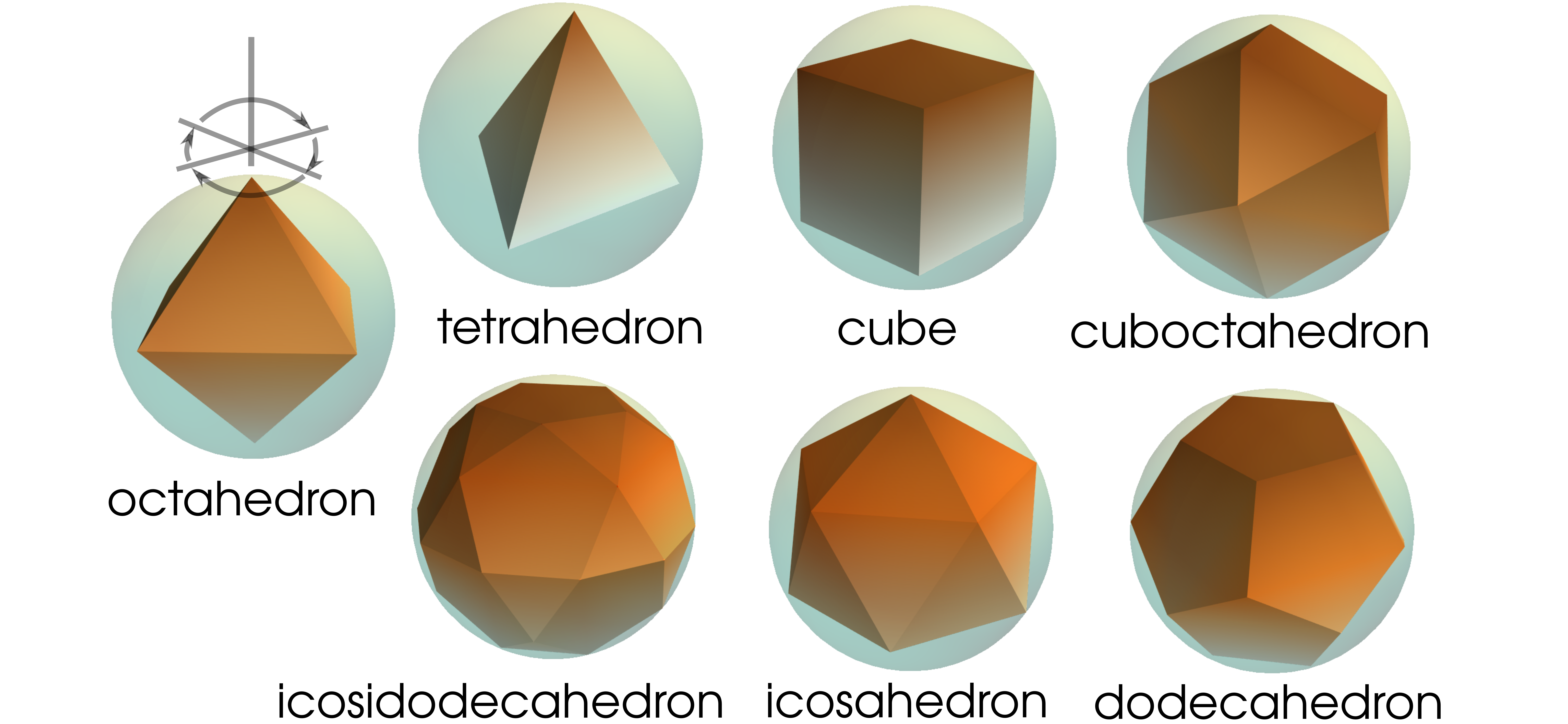
Figure 1: Example of generalised measurements defined by polytopes on the Bloch sphere: octahedron ($N=6$), tetrahedron ($N=4$), cube ($N=8$), cuboctahedron ($N=12$), icosahedron ($N=12$), dodecahedron ($N=20$), icosidodecahedron ($N=30$).

Repeating the measurement $M$ times on the system results in a string of outcomes $\{k_{i}\}_{i=1}^{M}$. Shadow tomography starts with associating a single outcome $k$ to a distribution $\vec{q}_{k}=\{\delta_{kl}\}_{l=1}^{N}$ in $\mathbb{R}^{N}$. Such a single data point can be used to obtain a noisy estimate of $\rho$, called classical shadow Aaronson (2020); Huang et al. (2020) , $\hat{\rho}_{k}=\chi(\vec{q}_{k})$. As a general strategy in data science, one can require the shadow estimator $\chi$ to be the least-square estimator, of which the solution is well-known Bishop (2006); Guţă et al. (2020) (see also (sup, , Appendix A)),

$$\chi_{\text{LS}}=(\Phi_{E}^{\dagger}\Phi_{E})^{-1}\Phi_{E}^{\dagger}.$$ (2)

Here we assume that the effects $\{E_{k}\}_{k=1}^{N}$ span the whole operator space, in which case $E$ is said to be informationally complete, so that $\Phi_{E}^{\dagger}\Phi_{E}$ is invertible. Notice that $\Phi^{\dagger}(\vec{q}_{k})=E_{k}$, and if we define $C_{E}=\Phi_{E}^{\dagger}\Phi_{E}$, then $C_{E}(\rho)=\sum_{k=1}^{N}\operatorname{Tr}(\rho E_{k})E_{k}$. The classical shadow can therefore also be written as

$$\hat{\rho}_{k}=C_{E}^{-1}(E_{k}).$$ (3)

The classical shadow in Eq. (3) resembles that in Ref. Huang et al. (2020). However, when the measurement is not ideal, the effects $E_{k}$ do not represent the state of the system after the measurement. In fact, unlike the procedure proposed in Ref. Acharya et al. (2021), our derivation suggests that the states of the system after the measurement is here not important (sup, , Appendix A-C).

Estimation of observables and the shadow norm— Each of the classical shadow (3) serves as an intermediate processed data point for further computation of observables. Given an observable $X$, each of the classical shadows $\hat{\rho}_{k}$ gives an estimate for the mean value $\langle X\rangle$ as $\hat{x}_{k}=\operatorname{Tr}(\hat{\rho}_{k}X)$. With the whole dataset $\{k_{i}\}_{i=1}^{M}$, the average $1/M\sum_{i=1}^{M}\hat{\rho}_{k_{i}}$ converges to $\rho$ (sup, , Appendix A), therefore $1/M\sum_{i=1}^{M}\hat{x}_{k_{i}}$ converges to $\langle X\rangle$. In this way, the mean value $\langle X\rangle$ can be estimated. For further refinement using the median-of-means estimation and estimation of polynomial functions of the density operator, see Ref. Huang et al. (2020). As also noted there, the asymptotic rate of convergence of the estimation is related to the variance of the estimator. For an observable $X$, the variance of the estimator can be computed as $\mathrm{var}(\hat{x}_{k})=\sum_{k=1}^{N}\operatorname{Tr}(\hat{\rho}_{k}X)^{2}\operatorname{Tr}(\rho E_{k})-\langle X\rangle^{2}$. Ignoring the second term results in an upper bound for the variance, and finally assuming the worst case scenario, i.e., maximisation over $\rho$, one arrives at the definition of the shadow norm of $X$ Huang et al. (2020),

$$\mathrm{var}({\hat{x}_{k}})\leq\left\|X\right\|_{E}^{2}=\lambda_{\max}\{\sum_{k=1}^{N}\operatorname{Tr}(\hat{\rho}_{k}X)^{2}E_{k}\}.$$ (4)

where $\lambda_{\max}\{\cdot\}$ denotes the maximal eigenvalue of the corresponding operator. The estimation procedure applies not only to an observable, but equally well to a set of observables $\mathcal{X}$. Assuming that the observables by certain normalisation all have the same physical unit, the quality of shadow tomography with a generalised measurement $E$ can be characterised by the maximal shadow norm,

$$\kappa_{E}^{2}(\mathcal{X})=\max\{\left\|X\right\|^{2}_{E}:X\in\mathcal{X}\}.$$ (5)

In the following, we would simply use $\kappa_{E}^{2}$ if the set of observables $\mathcal{X}$ is clear. Being the upper bound of the variance of the estimator, the smaller $\kappa_{E}^{2}$, the better is the estimator accuracy .

Symmetry of generalised measurements and the computation of the classical shadows— It has been observed that for certain classes of measurements, the inverse channel $C_{E}^{-1}$ is particularly simple Huang et al. (2020); Bu et al. (2022). We are to show that behind this simplicity is the symmetry of the generalised measurement Nguyen et al. (2020); Zhu and B. G. Englert (2011); Bogdanov et al. (2011).

To give the simple intuition, we discuss the example of the octahedron generalised measurement over a qubit plotted in Fig. 1, leaving the general argument for high dimensional cases in (sup, , Appendix E). Picking a vertex of the octahedron which corresponds to the effect $E_{k}$ in Fig. 1, we consider the symmetry rotations of the octahedron that leave this vertex invariant. These are rotations by multiples of $\pi/2$ around the axis going through the chosen vertex. Noticeably, there is a single projection (and its complement) that is invariant under these rotations, which corresponds to the state of the spin pointing to the vertex itself. In other words, the effect $E_{k}$ is uniquely specified by the symmetry. One can show that the corresponding classical shadow $\hat{\rho}_{k}$ is also invariant under these rotations, which then implies that it is a linear combination of $E_{k}$ and the identity operator $\openone$. In fact, this is a general property of the so-called uniform and rigidly symmetric measurements defined also for systems of general dimension $D$ sup ; Nguyen et al. (2020), which include in particular the symmetric solids in Fig. 1. In all these cases, one has

$$\hat{\rho}_{k}=aE_{k}+b\,\openone.$$ (6)

The coefficients $a$ and $b$ can be explicitly computed, $a=(D\beta-\alpha^{2})/(D\gamma-\alpha^{3})$ and $b=(\gamma-\alpha\beta)/(D\gamma-\alpha^{3})$, where $\alpha=\operatorname{Tr}(E_{k})$, $\beta=\operatorname{Tr}(E_{k}^{2})$, and $\gamma=\sum_{l=1}^{N}\operatorname{Tr}(E_{k}E_{l})^{2}$ (which are all independent of $k$).

Effects of noise in measurements— Measurements in realistic experimental setups aren’t ideal. The imperfection is due to various sources of noise in setting up the parameters of the measurement devices, or the resolution and the accuracy of readout signals Arute et al. (2019); Chen et al. (2019). As an example, suppose that the measurement $E$ is not perfectly implemented, where the device fails to couple to the system with probability $p$ and indicates an outcome at complete random. This can be modelled by the effects that are depolarised as $\{p\openone/N+(1-p)E_{k}\}_{k=1}^{N}$. Another example is the readout error, which is particularly important for superconducting qubits Bravyi et al. (2021); Hicks et al. (2022). In a simplified model, an outcome $0$ in the computational basis is misread as $1$ with probability $q_{+}$, and $1$ misread as $0$ with also probability $q_{-}$. The error rate averaged over the two bases is $\bar{q}=(q_{+}+q_{-})/2$ and the asymmetry between them is characterised by $\epsilon=(q_{+}-q_{-})/(q_{+}+q_{-})$. The measurement effects of the octahedron measurement implemented by randomisation under this noise becomes $1/3\{(1-q_{\pm})|t^{\pm}\rangle\langle t^{\pm}|+q_{\mp}|t^{\mp}\rangle\langle t^{\mp}|,t=x,y,z\}$. For further discussion, see (sup, , Appendix F).

Our formalism directly takes measurement error correction into account, once the noisy effects with an appropriate model are used instead of the ideal ones. To access the quality of the shadow tomography after error correction, we choose $\left|\mathcal{X}\right|=128$ pure state projections distributed according the Haar measure as observables. The dependence of the maximal shadow norm $\kappa_{E}^{2}$ on the noise parameters for the tetrahedron and the octahedron measurements is shown in Fig. 2. It is interesting to see that in either cases, the maximal shadow norm $\kappa_{E}^{2}$ depends only weakly on small error rate, showing the robustness of shadow tomography against noise.

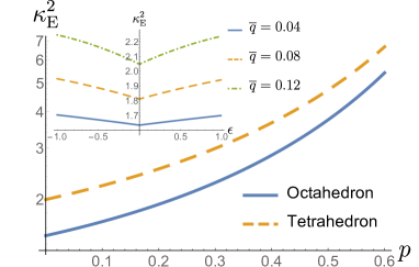
Figure 2: Effects of depolarisation noise (main) and simple readout error noise (inset) on the maximal shadow norm of $128$ pure state projections distributed according to the Haar measure.

Optimisation of generalised measurement for shadow tomography— Given a set of observables $\mathcal{X}$, one would like to find the generalised measurement $E$ so that the maximal shadow norm is minimised,

$$E^{\ast}=\arg\min_{E}\kappa_{E}^{2}(\mathcal{X}).$$ (7)

Restricted to randomised unitaries, this optimisation is impractical to carry out (sup, , Appendix B). Extending to all generalised measurements, this is simply an optimisation over a convex domain. We implemented simulated annealing for the minimisation and found the obtained optima to be highly reliable (sup, , Appendix G). Below we start with discussing the case of a single qubit, which, despite being simple, is also the basis to understand the case of many qubits.

Example 1.

Consider a single qubit. As for the observables $\mathcal{X}$, we consider the following possibilities: (a) Take observables to be $4$ projections corresponding to the orange tetrahedron in Fig. 3a. The squared shadow norm $\kappa_{E}^{2}$ is $2$ for the tetrahedron generalised measurement defined exactly by these $4$ projections, and $3/2$ for the octahedron measurement. The optimiser suggests that the tetrahedron measurement plotted in violet in Fig. 3a, obtained by centrally inverting the orange tetrahedron, is optimal with $\kappa_{E}^{2}=1$. (b) As observables consider the projections onto the eigenstates of the Pauli observables, see the orange octahedron in Fig. 3b. The octahedron measurement itself gives $\kappa_{E}^{2}=3/2$. Interestingly, the optimiser shows that $\kappa_{E}^{2}=3/2$ can also be obtained with the tetrahedron generalised measurement of $4$ outcomes indicated in violet in Fig. 3b. (c) Lastly, as observables we consider random projections distributed according to the Haar measure on the Bloch sphere. Fig. 3c presents the shadow norms obtained by the optimiser with respect to the number of observables. For small number of observables ($\left|\mathcal{X}\right|\lesssim 15$), the optimiser always finds measurements with a given number of outcomes significantly better than the standard tetrahedron ($N=4$) or the octahedron measurements $(N=6)$. It is interesting to see that if the number of outcome is fixed to be $6$ or $8$, the $\kappa_{E}^{2}$ converges to the octahedron measurement with the value of $3/2$.

The last example (c) hints that the octahedron measurement is somewhat special. Indeed, it turns out the squared shadow norm with respect to the octahedron measurement for any projection is identically $3/2$. Using this fact, we show that if the targeted observables are all the projections on arbitrary pure states of the qubit, the optimal measurement would be the octahedron measurement assuming equal trace of the effects (sup, , Appendix H).

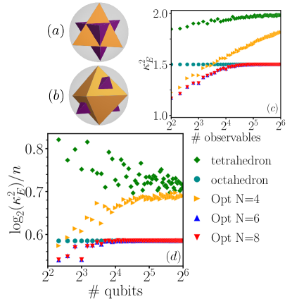
Figure 3: Targeted observables and optimal generalised measurements. (a) For observables corresponding to four projections defined by the orange tetrahedron, the measurement corresponding to the inverted tetrahedron measurement (violet) is optimal. (b) For observables corresponding to eigenprojections of the Pauli observables $\sigma_{x}$, $\sigma_{y}$ and $\sigma_{z}$ (orange octahedron), the violet tetrahedron measurement is optimal. (c) Optimal shadow norms given by the optimiser (labelled Opt with the number of measurement outcomes) as a function of the number of single-qubit projection observables randomly distributed according to the Haar measure. (d) Similarly, optimal shadow norms given by the optimiser as a function of the number of qubits. The observables are tensor products of single-qubit projections distributed according to the Haar measure. In (c) and (d), the shadow norm for the tetrahedron and octahedron measurements are also shown.

Tensoring the shadow construction for many-body systems— Shadow tomography is especially designed for the cases where the system size is large. Consider the case where the system consists of $n$ qubits, corresponding to the total dimension of $D=2^{n}$. In this case, shadow tomography can be performed by making (identical or not identical) generalised measurements $\{E^{(1)},E^{(2)},\ldots,E^{(n)}\}$ on each of the qubit, each described by a collection of $N_{i}$ effects, $E^{(i)}=\{E^{(i)}_{k}\}_{k=1}^{N_{i}}$. Theoretically, this corresponds to a measurement of a generalised measurement $E^{\text{tot}}$ on the whole system with each effect labelled by a string of outcomes $\boldsymbol{k}=\{k^{(1)},k^{(2)},\ldots,k^{(n)}\}$, $E^{\text{tot}}_{\boldsymbol{k}}=E^{(1)}_{k^{(1)}}\otimes E^{(2)}_{k^{(2)}}\otimes\cdots\otimes E^{(n)}_{k^{(n)}}$. The whole general analysis above can be applied. In fact, such a string $\boldsymbol{k}$ of outcomes corresponds simply to the classical shadow

$$\hat{\rho}^{\text{tot}}_{\boldsymbol{k}}=\hat{\rho}_{k^{(1)}}^{(1)}\otimes\hat{\rho}_{k^{(2)}}^{(2)}\otimes\cdots\otimes\hat{\rho}_{k^{(n)}}^{(n)},$$ (8)

where $\hat{\rho}^{(i)}_{k^{(i)}}$ being the classical shadow corresponding to the measurement $E^{(i)}$ on the $i$-th qubit. Crucially, the typical observables of the system can be easily estimated without (impractically) explicitly computing the classical shadows in the form of a $D\times D$ matrix Huang et al. (2020). Indeed, an observable $X$ on the system is often of the form $X=X^{(1)}\otimes X^{(2)}\otimes\cdots\otimes X^{(n)}$. Then, a single string of outcomes $\boldsymbol{k}$ gives rise to a single estimate of $\langle X\rangle$ as $\operatorname{Tr}[\hat{\rho}^{(1)}_{k^{(1)}}X^{(1)}]\,\operatorname{Tr}[\hat{\rho}^{(2)}_{k^{(2)}}X^{(2)}]\,\cdots\operatorname{Tr}[\hat{\rho}^{(n)}_{k^{(n)}}X^{(n)}]$. The final estimate of $\langle X\rangle$ is as usual obtained by averaging over all data points. Observe that it is not necessary to construct the large density operator of the whole system. Moreover, the shadow norm of such a factorised observable also factorises $\left\|X\right\|_{E}=\left\|X^{(1)}\right\|_{E^{(1)}}\left\|X^{(2)}\right\|_{E^{(2)}}\cdots\left\|X^{(n)}\right\|_{E^{(n)}}$.

Optimising generalised measurements for many-body systems— For many qubits, the number of parameters to be optimised in Eq. (7) increases exponentially. To simplify, one can assume that for a many-qubit system, the generalised measurement is factorised as a tensor product over the qubits as we discussed above. Moreover, if there is no preference among the qubits, one can also assume that, $E^{(1)}=E^{(2)}=\cdots=E^{(n)}$. The complexity of the computation under these assumptions is only linear in the number of qubits and the number of observables.

Example 2.

We consider a system of upto $n=64$ qubits. We choose $\left|X\right|=n$ observables which are products of different component observables on single qubits. The component observables on single qubits are randomly distributed according to the Haar measure. As the qubits are equivalent, one might anticipate that the optimal factorising measurement for the qubits is similar to those that are optimised separately for each qubit. Our simulations confirm this expectation. In Fig. 3d, for small number of qubits ($n\lesssim 10$), the optimiser with $N=6$ and $N=8$ gives significantly lower shadow norms for the choice of tetrahedron or octahedron measurements. On the other hand, observe that as the number of qubits increases, the obtained optimal shadow norm converges to that given by the octahedron measurement, pointing to the speciality of the octahedron measurement on qubit-based platforms as we discussed in Example 1 (c).

Conclusion— Being both more general and simpler, the formulation of shadow tomography with generalised measurements sheds light on various aspects of shadow tomography. This also opens a range of interesting questions for future research. Further analysis of realistic noise in the existing and future experiments Fischer et al. (2022); Stricker et al. (2022) of shadow tomography could be considered. Extension of this framework to channel tomography is of direct interest. It would be also important to see whether the technique of derandomisation Huang et al. (2021) can also be incorporated. The optimality of the octahedron measurement for shadow tomography for qubit-based system suggests a connection between geometry and shadow tomography. Investigation of this connection and extension for higher dimensional systems would be an interesting direction. Also the construction of optimal measurements for nonlinear functions of the density operator, or shadow tomography of a specific set of density operators, is in demand for further applications of shadow tomography.

See pages 1, of shadow-tomography-appendix.pdf See pages 2, of shadow-tomography-appendix.pdf See pages 3, of shadow-tomography-appendix.pdf See pages 4, of shadow-tomography-appendix.pdf See pages 5, of shadow-tomography-appendix.pdf See pages 6, of shadow-tomography-appendix.pdf