Price Interpretability of Prediction Markets: A Convergence Analysis

Abstract.

Prediction markets are long known for prediction accuracy. This study systematically explores the fundamental properties of prediction markets, addressing questions about their information aggregation process and the factors contributing to their remarkable efficacy. We propose a novel multivariate utility (MU) based mechanism that unifies several existing automated market-making schemes. Using this mechanism, we establish the convergence results for markets comprised of risk-averse traders who have heterogeneous beliefs and repeatedly interact with the market maker. We demonstrate that the resulting limiting wealth distribution aligns with the Pareto efficient frontier defined by the utilities of all market participants. With the help of this result, we establish analytical and numerical results for the limiting price in different market models. Specifically, we show that the limiting price converges to the geometric mean of agent beliefs in exponential utility-based markets. In risk-measure-based markets, we construct a family of risk measures that satisfy the convergence criteria and prove that the price can converge to a unique level represented by the weighted power mean of agent beliefs. In broader markets with Constant Relative Risk Aversion (CRRA) utilities, we reveal that the limiting price can be characterized by systems of equations that encapsulate agent beliefs, risk parameters, and wealth. Despite the potential impact of traders’ trading sequences on the limiting price, we establish a price invariance result for markets with a large trader population. Using this result, we propose an efficient approximation scheme for the limiting price. Numerical experiments underscore the accuracy of this approximation across various scenarios, outperforming existing approximation methods. Our findings serve to aid market designers to better tailor and adjust the market-making mechanism for more effective opinions elicitation.

1. Introduction

Information, often scattered among the crowd, is valuable yet hard to aggregate. Throughout the centuries, researchers and practitioners have invented various tools in an attempt to piece them together. Classical mechanisms like polls, surveys, and brainstorming work fine. However, they lack the commitment to let people put their money where their mouth is. Over the past two decades, the prediction market, a mechanism designed specifically for information elicitation and aggregation, has gained much popularity. For example, the Iowa Electronic Markets (IEM), arguably the pioneer of all existing prediction markets designed primarily for various elections, almost consistently beats professional opinion polls (Berg et al., 2008). Other success stories include corporate consensus pooling, box office forecasting, and online recreational sports betting (e.g., (Chen et al., 2005; Cowgill et al., 2009; Cogwill and Zitzewitz, 2015)). There is theoretical evidence that prediction markets are robust against price manipulation (Hanson and Oprea, 2009). Overall, prediction markets have become a popular tool for information aggregation (e.g., (Wolfers and Zitzewitz, 2004; Arrow et al., 2008)).

Due to the liquidity issue, a prediction market is usually organized by an automated market maker (Hanson, 2003). In this market, traders exchange specialized securities with a market maker. These securities offer rewards based on uncertain outcomes, revealed once the true state is known. Traders, guided by their subjective beliefs, trade with the market maker to gain expected utility. Simultaneously, the market maker gathers valuable information through trading to enhance the overall accuracy of predictions. While the prediction market literature has primarily focused on designing effective market-making mechanisms (e.g., (Chen and Pennock, 2007; Abernethy et al., 2013; Othman et al., 2013; Slamka et al., 2013)), there have been relatively few attempts to explore the market’s evolutionary behavior. In this paper, we aim to narrowing this gap by addressing the following questions and providing additional insights into the analysis of prediction markets.

1. Under what conditions can we expect a prediction market to reach a consensus? That is, when does the trading process (market price) converge?

2. How to interpret the limiting price? What is the relation between such limiting price with each trader’s belief, wealth and their risk attitude?

In line with the spirit of (Sethi and Vaughan, 2016), we explore a dynamic prediction market model with multiple securities, involving a finite number of myopic, risk-averse traders with heterogeneous beliefs interacting with an automated market maker. We make several contributions that enhance the understanding and effectiveness of prediction markets.

Firstly, we introduce a unified multivariate utility (MU)-based mechanism that incorporates several market making mechanisms (e.g., (Hanson, 2003, 2007; Chen and Pennock, 2007; Agrawal et al., 2011)) into a consistent framework. Based on this framework, we propose a method for establishing market convergence that subsumes and extends the existing results in (Frongillo et al., 2015) and (Sethi and Vaughan, 2016). More importantly, we demonstrate that the limiting wealth distribution is Pareto optimal with respect to the utility of each trader. Additionally, this approach allows us to bypass the challenges of analyzing transient behavior in price dynamics and enables a direct examination of the limiting price.

By leveraging the general convergence result, we study the convergence properties of various utility types. Specifically, we derive the analytical form of price dynamics for the exponential utility-based market, revealing that the limiting price is the geometric mean of agents’ beliefs and is independent of the trading sequences. We extend this result to the convex risk-measure-based market. Specifically, we present an explicit method to construct risk measures that satisfy the convergence requirements. For a wide range of convex risk measures, we derive the analytical form of the limiting price, which emerges as a weighted power mean of agent beliefs.

Furthermore, we explore the more commonly used market model where all participants adopt the utility with constant relative risk aversion (i.e., CRRA utility) to make decisions. We analyze traders’ optimal trading decisions and examine the limiting wealth distribution resulting from the aggregate Pareto-optimization problem. It reveals that the limiting price can be characterized through a system of equations including all participants’ risk parameters, initial wealth allocation, and subjective beliefs. Crucially, we establish a fundamental result indicating that, even though trading sequences can influence the limiting price, their impact diminishes to insignificance as the trader population increases. Using these results, we introduce a heuristic weight called Pareto Optimal Induced (POI) weights and derive the associated approximate price formula that underscores the important role of risk aversion and initial wealth in price determination. To evaluate this approximation scheme, we conduct numerical experiments, which demonstrate that our POI price can closely track the actual price resulting from the trading with high accuracy across various settings. Through further comparison, our approximation scheme consistently outperforms previous attempts in the literature, such as the one presented in (Sethi and Vaughan, 2016). This performance improvement significantly advances the state-of-the-art in our comprehension of market prices.

Our findings hold significant potential for various applications. Firstly, the MU-based mechanism offers extensive flexibility in designing pricing formulations, empowering the market designer to tailor markets for diverse purposes. Secondly, our theoretical results establish a link between the parameters and the limiting price, enhancing the market designer’s ability to elicit traders’ beliefs effectively. Specifically, this suggests that market maker should exercise caution when selecting risk and wealth parameters to balance liquidity and accuracy. Our theoretical result on price stability in a random trading market suggests attracting more traders to achieve a reliable limiting price. Moreover, in scenarios like artificial prediction markets ((Chakravorti et al., 2023)), where traders are artificially generated supervised learners, our results provide guidance for configuring hyper-parameters for these artificial traders. Lastly, our convergence scheme and the subsequent price analysis can be effortlessly extended to prediction markets without a market maker. As an ancillary outcome, the theoretical proof of market convergence is closely related to the distributional algorithm of weakly-coupled multi-objective optimization. This proof can be extended to address more generalized problems sharing a similar structure.

This paper is organized as follows. In the remainder of this section, we review the related literature. In Section 2, we introduce the market model and the multivariate utility (MU)-based pricing mechanism. In Section 3, we present the general convergence result. In Section 4, we study the exponential utility-based market and the risk measure-based market. We then explore the CRRA utility-based market in Section 5. In Section 6, we discuss the price-volume relationship and the non-stationary market setting. We conclude the paper in Section 7. All the proofs and related results are provided in the Appendix.

1.1. Related Research

Our work is closely related to the research on automated market-making mechanisms in prediction markets. The logarithm market scoring rule (LMSR) introduced by (Hanson, 2003, 2007), stands out as one of the most popular mechanisms in internet prediction markets due to its desirable properties. In practice, LMSR can be implemented in the form of a cost function (Chen and Vaughan, 2010). This cost function-based mechanism has been refined in various directions (e.g., (Othman et al., 2013; Abernethy et al., 2013, 2014b)). Furthermore, (Chen and Pennock, 2007) propose a univariate utility function-based framework, which strongly motivates our adoption of the multivariate utility (MU)-based mechanism. Additionally, (Agrawal et al., 2011) introduce the sequential convex pari-mutuel mechanisms, allowing the market to accept limit orders. Partial equivalence among these mechanisms has been established (Chen and Pennock, 2007; Chen and Vaughan, 2010; Agrawal et al., 2011). To deal with the liquidity-adaption problem in practical implementation, (Othman et al., 2013) propose a liquidity-sensitive mechanism. Recent developments have extended these mechanisms in various directions (e.g., (Freeman et al., 2017; Ban, 2018; Freeman and Pennock, 2018)). As for the performance comparison of different mechanisms, (Slamka et al., 2013) provide simulation studies.

In prediction markets, trading-generated prices serve as predictors of future events, reflecting an aggregate estimate of the likelihood of a certain event occurring ((Manski, 2006; Wolfers and Zitzewitz, 2006)). As for the market convergence and price interpretation, there are generally two streams of studies. The first one involves a common prior and heterogeneous information. (Ostrovsky, 2012) and (Iyer et al., 2014) find that when all participants are risk-neutral or risk-averse, prices converge to a common posterior. These findings align with the well-known theorem established by (Aumann, 1976), stating that people with a common prior must have a common posterior if all posteriors are common knowledge, or in short, people cannot agree to disagree. The second stream of the model is characterized by heterogeneous priors but common information. In this model, several researchers adopt the static equilibrium model, where the price results from the market clearing condition. Following this idea, (Gjerstad and Hall, 2005) and (Manski, 2006) find a bias between traders’ mean beliefs and the equilibrium price. However, (Pennock, 1999) and (Wolfers and Zitzewitz, 2006) show that the market equilibrium coincides with the wealth-weighted average of trader’s beliefs when traders adopt the logarithm utility to make decisions.

In contrast to the above static model, another line of research explores the dynamic trading model. (Othman and Sandholm, 2010) investigate a market with risk-neutral traders with heterogeneous beliefs. In this setting, a finite number of traders interact with the market only once, resulting in a dependence between the trading order and the last posted price. In a related study, (Frongillo and Reid, 2015) adopt risk measures to model traders’ preferences in a market equipped with a cost function-based mechanism. When the traders trade with the market maker in random order, the dynamic trading process exhibits similarities with a machine learning algorithm that aims to minimize aggregate risk. While they develop some convergence conditions, their approach critically relies on the translation invariance property of risk measures ((Föllmer and Knispel, 2015)), which cannot be directly applied in our general MU-based market. Our work shares more similarities with (Sethi and Vaughan, 2016), who establish price convergence for a binary predication market with risk-averse traders and an LMSR-based market maker. However, our research focuses on a broader market setting, encompassing multiple securities, a general market-making mechanism, and a variety of trading decision paradigms. These complexities make it challenging to apply their approaches effectively to analyze our general model. We also note that (Bonnisseau and Nguenamadji, 2013) have considered a discrete Walrasian process, which is related to our model. However, the key difference is that their process involves pure exchange without a market maker. In contrast, our model is more intricate due to the externality introduced by the market maker and the pairwise trading restriction. The conditions required for market convergence in this scenario remain unclear, which partially motivates our current research.

Additionally, several studies have examined prediction markets with specific market structures. For example, (Abernethy et al., 2014a) analyze the equilibrium properties of a market with traders whose beliefs are drawn from exponential family distributions. (Carvalho, 2017) demonstrates that in a binary prediction market with an LMSR-based mechanism and risk-neutral budget-constrained traders, the price converges to the median belief of traders. (Tarnaud, 2019) investigates the asymptotic properties of a simple binary market with an LMSR-based mechanism and two traders. As valuable tools for forecasting and information aggregation, prediction markets also receive attention in the operations research and management science societies. For example, (Chen et al., 2008) develop a diffusion model for predicting the price of political events in prediction markets, while (Berg et al., 2009) use prediction markets to forecast market capitalization before an initial public offering. (Healy et al., 2010) investigate different trading mechanisms in small markets with complex environments. (Atanasov et al., 2017, 2022) systematically compare prediction markets with other popular information elicitation methods. Through several large-scale experimental tests, they find these two methods have advantages in different situations. (Jian and Sami, 2010) and (Choo et al., 2022) study the accuracy of prediction markets when there is price manipulation.

Besides the human-populated markets, artificial prediction markets with artificial agents (bot-traders) are developed as supervised learning tools for probability estimation and the aggregation of weak classifiers (e.g., (Storkey et al., 2012; Chakravorti et al., 2023)). Tuning the hyper-parameters (i.e., wealth, risk parameter, and beliefs of each bot-trader) in these artificial markets is a key challenge, as highlighted by (Chakravorti et al., 2023). Our convergence result and interpretation of the limiting price provide potential guidance for tuning these hyper-parameters.

Notations: A vector is denoted by a boldface letter, i.e., $\mathbf{x}=(x_{1},\ldots,x_{n})\in\mathbb{R}^{n}$ stands for a column vector $\mathbf{x}$. Let $\mathbf{e}$ and $\mathbf{0}$ be the all-one and all-zero vectors in the appropriate dimension, respectively. Given vectors $\mathbf{y}$ and $\mathbf{x}$ in $\mathbb{R}^{n}$, the notation $\mathbf{y}\geq\mathbf{x}$ means that $y_{i}\geq x_{i}$ for all $i$, while $\mathbf{y}>\mathbf{x}$ indicates that $\mathbf{y}\geq\mathbf{x}$ and there exists an $i$ such that $y_{i}>x_{i}$. Notations $\mathrm{recc}(\mathcal{A})$ and $\mathrm{recc}(F)$ represent the recession cone of the convex set $\mathcal{A}$ and the convex function $F$, respectively (as defined in Bertsekas et al. 2003). The domain of function $F(\cdot)$ is denoted as $\textbf{{dom}}(F)$, and the probability simplex is represented as $\Theta_{n}\triangleq\{(q_{1},\ldots,q_{n})\in\mathbb{R}^{n}_{+}|\sum_{i=1}^{n}q_{i}=1\}$, where $\mathbb{R}_{+}$ denotes the set of nonnegative real numbers.

2. Market Model and Trading Process

In this section, we introduce the market model. We consider a state space $\{1,2,\ldots,I\}$ with $I\geq 2$, comprising mutually exclusive and exhaustive outcomes. Each state $i\in\{1,2,\ldots,I\}$ corresponds to an Arrow-Debreu security, which pays $1$ dollar if state $i$ occurs. These securities are traded in a prediction market organized by a central market maker. A total of $J>1$ traders engage in repeated transactions with the market maker at discrete time points $t=0,1,2,\ldots$. We represent the market maker’s wealth at time $t$ as $W_{t}\in\mathbb{R}$ and their outstanding securities position (i.e., the number of securities already sold) as $\mathbf{Q}_{t}\in\mathbb{R}^{I}$. The market maker’s initial values are $W_{0}>0$ and $\mathbf{Q}_{0}=\mathbf{0}$. For each trader indexed by $j=1,\ldots,J$, we use $w_{j,t}\in\mathbb{R}$ and $\mathbf{q}_{j,t}\in\mathbb{R}^{I}$ to denote their wealth and security positions at time $t=0,1,2,\ldots$. The initial values are $w_{j,0}>0$ and $\mathbf{q}_{j,0}=\mathbf{0}$.

At each time $t$, one trader interacts with the market maker (we will specify the order of arrivals of the traders in later discussions) by submitting an order $\Delta\mathbf{q}\in\mathbb{R}^{I}$. For instance, in the context of a football match outcome, such an order might be expressed as $\Delta\mathbf{q}=(2,1,-1)$, representing $2$ shares for a buying order on “win”, $1$ share for a buying order on “loss”, and $1$ share for a selling order on “tie”. At any time $t$, if the $j$-th trader pays $\Delta w$ to the market marker (if $\Delta w<0$, then it means the trader is paid $-\Delta w$ by the market maker) and buys $\Delta\mathbf{q}$ share of security, then the market state is updated as follows:

(1) $$\textrm{Trader $j$:}\begin{dcases}w_{j,t+1}=w_{j,t}-\Delta w\\ \mathbf{q}_{j,t+1}=\mathbf{q}_{j,t}+\Delta\mathbf{q}\end{dcases},~{}~{}~{}~{}~{}\textrm{Market Maker:}\begin{dcases}W_{t+1}=W_{t}+\Delta w\\ \mathbf{Q}_{t+1}=\mathbf{Q}_{t}+\Delta\mathbf{q}.\end{dcases}$$

The other traders’ positions keep unchanged, i.e., $w_{k,t+1}=w_{k,t}$ and $\mathbf{q}_{k,t+1}=\mathbf{q}_{k,t}$, for $k=1,\ldots,J$ and $k\not=j$.

To price an order $\Delta\mathbf{q}\in\mathbb{R}^{I}$, the market maker adopts a multivariate-utility (MU)-based mechanism described as follows. Suppose the market marker’ MU function is $U(\cdot):\mathbb{R}^{I}\rightarrow\mathbb{R}$, which maps the net wealth position $\mathbf{y}_{t}\triangleq W_{t}\cdot\mathbf{e}-\mathbf{Q}_{t}\in\mathbb{R}^{I}$ to some real value. We call $\mathbf{y}_{t}$ the net wealth position because it represents all the possible wealth level if the final state is revealed at time $t$. Similar to the utility-based pricing mechanism in (Chen and Pennock, 2007), the price of the order $\Delta\mathbf{q}$ is determined by solving the following optimization problem:

$$\mathcal{P}_{\textrm{cmin}}(\Delta\mathbf{q}):~{} ~{}\min_{\Delta w\in\mathbb{R}}~{}~{}\Delta w$$

(2) Subject to: $$~{}U\big{(}(W_{t}+\Delta w)\cdot\mathbf{e}-(\mathbf{Q}_{t}+\Delta\mathbf{q})\big{)}\geq U(W_{0}\cdot\mathbf{e}),$$

$$~{}(W_{t}+\Delta w)\cdot\mathbf{e}-(\mathbf{Q}_{t}+\Delta\mathbf{q})\in\textbf{{dom}}(U).$$

The minimizer of problem $\mathcal{P}_{\textrm{cmin}}(\Delta\mathbf{q})$ is the price of the order $\Delta\mathbf{q}$. Constraint (2) can also be written as $U(\mathbf{y}_{t}+(\Delta w\cdot\mathbf{e}-\Delta\mathbf{q}))\geq U(W_{0}\cdot\mathbf{e})$, which means that the utility of the updated net wealth position is no less than that of the initial state. This is consistent with the utility-preserving property proposed in (Chen and Pennock, 2007), i.e., the market maker tries to find the lowest possible charge for the order $\Delta\mathbf{q}$ such that the post-trade utility level is no less than the initial level.

To ensure the above pricing problem is well-posed, throughout this paper, we assume $U(\cdot)$ satisfies the following assumptions.

Assumption 1.

$U(\cdot)$ satisfies the following conditions: (i) it is continuous, concave and its domain $\textbf{{dom}}(U)$ is convex with $\mathbf{e}\in\mathrm{recc}(\textbf{{dom}}(U))$; (ii) it is monotonically increasing.

Assumption 1 is mild and natural for the utility function except for the requirement $\mathbf{e}\in\textrm{recc}(\textbf{{dom}}(U))$ which means that the utility is well-defined even if the wealth goes to infinity. Under Assumption 1, it can be verified that the MU-based pricing rule satisfies the axioms proposed in (Abernethy et al., 2013). These axioms serve as general requirements for a reasonable pricing mechanism. Furthermore, the MU-based pricing rule possesses several other desirable properties. For instance, it demonstrates responsiveness to any finite order with a unique price, effectively eliminates arbitrage opportunities for surebets, and exhibits a finite worst-case loss (under mild conditions). Moreover, there is abundant freedom to construct MU functions (see examples in Appendix B.1). The following result establishes the relation between the MU-based pricing rule with the MSR and the cost function-based mechanism.

Proposition 2.1.

An MU-based mechanism with a utility function satisfying Assumption 1 is equivalent with a cost function-based mechanism with a corresponding cost function. Furthermore, if an MU-based mechanism has a bounded loss under worst-case scenario, then the underlying utility can induce a proper scoring rule. Conversely, any proper scoring rule can induce an MU-based mechanism that has bounded worst-case loss.

The detailed proof of the above proposition is provided in Appendix B.2. In this work, we adopt the MU-based pricing rule in our analysis mainly due to the following reasons. First, as shown in Proposition 2.1, the MU-based pricing rule is general enough to cover existing classical pricing rules. More importantly, the MU-based mechanism provides a tractable way to study the convergence property of prices generated by a dynamic trading process. Once we have these convergence results, they can be directly applied to other pricing rules. Second, compared with the cost function-based pricing rule (Chen and Pennock, 2007; Abernethy et al., 2013) and the LMSR (Hanson, 2003), the MU-based mechanism could explicitly incorporate the risk preferences and the heterogeneous beliefs of all participants in a unified framework, which enables us to explore how these heterogeneous factors affect the final prices of these securities. Third, it is more convenient to construct the MU function in practice compared with the other mechanisms. For example, using risk-measure to define the cost function needs it to be convex and translation invariant, which means that the cost function should not be strictly convex. Indeed, it is usually not an easy task to customize a valid cost function in an analytical form. In contrast, the MU-based utility only requires the function to be concave and monotone, and it can be constructed in various ways, including the classic expected utility theory (EUT) (Chen and Pennock, 2007) and convex risk measures (e.g., (Chen and Pennock, 2007; Föllmer and Schied, 2011; Hu and Storkey, 2014; Frongillo et al., 2015)). Moreover, the price of an order can be computed by a simple line search. We provide additional properties of the MU function and some examples in Appendix B.

On the trader’s side, we assume that each trader $j\in\{1,\ldots,J\}$ also adopts an MU function, $V_{j}(\cdot):\mathbb{R}^{I}\rightarrow\mathbb{R}$, to evaluate his/her net wealth position. Following the spirit of (Sethi and Vaughan, 2016), the $j$-th trader solves the following problem to decide the amount of securities to trade,

$$\bar{\mathcal{P}}_{j}(w_{j,t},\mathbf{q}_{j,t}):~{} ~{}\max_{\Delta\mathbf{q}\in\mathbb{R}^{I},~{}\Delta w\in\mathbb{R}}~{}~{}V_{j}\big{(}(w_{j,t}-\Delta w)\cdot\mathbf{e}+(\mathbf{q}_{j,t}+\Delta\mathbf{q})\big{)}$$

subject to $$~{}\Delta w=\arg\min_{w\in\mathbb{R}}~{}\big{\{}w~{}|~{}U\big{(}(W_{t}+w)\cdot\mathbf{e}-(\mathbf{Q}_{t}+\Delta\mathbf{q})\big{)}\geq U(W_{0}\cdot\mathbf{e}),$$

$$~{}~{}~{}~{}~{}~{}~{}~{}~{}~{}~{}~{}~{}~{}~{}(W_{t}+w)\cdot\mathbf{e}-(\mathbf{Q}_{t}+\Delta\mathbf{q})\in\textbf{{dom}}(U),$$

(3) $$~{}~{}~{}~{}~{}~{}~{}~{}~{}~{}~{}~{}~{}~{}~{}(w_{j,t}-w)\cdot\mathbf{e}+(\mathbf{q}_{j,t}+\Delta\mathbf{q})\in\textbf{{dom}}(V_{j})\big{\}}.$$

In this problem, the term $(w_{j,t}-\Delta w)\cdot\mathbf{e}+(\mathbf{q}_{j,t}+\Delta\mathbf{q})$ in the objective function represents the $j$-th trader’s net wealth position after the current trading. Problem $\bar{\mathcal{P}}_{j}(w_{j,t},\mathbf{q}_{j,t})$ can be viewed as a bi-level optimization problem. It fully characterizes all the information in one round of trading, i.e., the size of the order $\Delta\mathbf{q}$ is determined by the upper-level problem, and the payment of the order $\Delta\mathbf{q}$, is determined by the subproblem in constraint (3). The lower level subproblem in constraint (3) is nothing but the problem $\mathcal{P}_{\textrm{cmin}}(\Delta\mathbf{q})$. To guarantee the whole trading process is well defined, we impose the following conditions for $V_{j}(\cdot)$, $j=1,\ldots,J$.

Assumption 2.

Each $V_{j}(\cdot)$ satisfies the following conditions: (i) it is continuous and strictly concave for non-equivalent wealth vectors; (ii) $\textbf{{dom}}(V_{j})$ is convex with $\mathrm{recc}(V_{j})\subseteq\mathbb{R}^{I}_{+}$ and $\mathbf{e}\in\mathrm{recc}(\textbf{{dom}}(V_{j}))$; (iii) it is monotonically increasing.

Assumption 2 is similar to Assumption 1 except that it requires $V_{j}(\cdot)$ to be strictly concave except along the direction $\mathbf{e}$. This condition is necessary to establish trading process convergence in the later part of this paper. Note that such an assumption is weaker than global strict concavity, and it can also accommodate risk measure-based MU function, which is linear along direction $\mathbf{e}$.

Although the state $\{w_{j,t},\mathbf{q}_{j,t}\}$ fully represents the trading process, it is complicated to study the convergence of the trading process by solving problem $\bar{\mathcal{P}}_{j}(w_{j,t},\mathbf{q}_{j,t})$ directly. It is more convenient to use the net wealth position to characterize the trading process. Specifically, at time $t$, let $\mathbf{x}_{j,t}\triangleq w_{j,t}\cdot\mathbf{e}+\mathbf{q}_{j,t}$ and $\mathbf{y}_{t}\triangleq W_{t}\cdot\mathbf{e}-\mathbf{Q}_{t}$ be the $j$-th trader’s and the market maker’s net wealth position, respectively. At time $t=0$, it has $\mathbf{x}_{j,0}=w_{j,0}\cdot\mathbf{e}$ and $\mathbf{y}_{0}=W_{0}\cdot\mathbf{e}$. In each round of trading, when an order $\Delta\mathbf{q}$ is placed at price $\Delta w$, the variation of market maker’s wealth is denoted as $\mathbf{z}\triangleq\big{(}z_{1},z_{2},\ldots,z_{I}\big{)}=-\Delta w\cdot\mathbf{e}+\Delta\mathbf{q}$. Then, the dynamics (1) transform into $\mathbf{x}_{j,t+1}=\mathbf{x}_{j,t}+\mathbf{z}$ if the $j$-th trader interacts with the market at time $t$, and $\mathbf{x}_{k,t+1}=\mathbf{x}_{k,t}$ for $k\not=j$, along with the market maker’s wealth update, $\mathbf{y}_{t+1}=\mathbf{y}_{t}-\mathbf{z}$. It is worth noting that the market total wealth adheres to the following condition:

(4) $$\mathbf{y}_{t}+\sum_{j=1}^{J}\mathbf{x}_{j,t}=\sum_{j=1}^{J}\mathbf{x}_{j,0}+\mathbf{y}_{0}={w}^{\textrm{all}}_{0}\cdot\mathbf{e},$$

for all $t=0,1,\ldots$, where ${w}^{\textrm{all}}_{0}\triangleq\sum_{j=1}^{J}w_{j,0}+W_{0}$ is the total wealth of all participants in the market. Eq. (4) suggests that the total net wealth position in the market maintains at a constant level throughout the trading process.

Using the wealth vectors $\mathbf{x}_{j,t}$ and $\mathbf{y}_{t}$, the utility preserving property (2) can be expressed as $U\big{(}\mathbf{y}_{t}-\mathbf{z})\geq U(W_{0}\cdot\mathbf{e})$. This formulation motivates us to consider an equivalent formulation of the $j$-th trader’s decision problem:

$$\mathcal{P}_{j}(\mathbf{x}_{j,t}):~{}~{}\max_{\mathbf{z}\in\mathbb{R}^{I}}~{} ~{}V_{j}(\mathbf{x}_{j,t+1})=V_{j}(\mathbf{x}_{j,t}+\mathbf{z})$$

(5) Subject to: $$~{}U(\mathbf{y}_{t}-\mathbf{z})\geq U(W_{0}\cdot\mathbf{e}),$$

$$~{}\mathbf{y}_{t}-\mathbf{z}\in\textbf{{dom}}(U),~{}\mathbf{x}_{j,t}+\mathbf{z}\in\textbf{{dom}}(V_{j}),$$

for given $\mathbf{x}_{j,t}$ and $\mathbf{y}_{j,t}$ satisfying (4). The following result establishes equivalence between problems $\mathcal{P}_{j}(\mathbf{x}_{j,t})$ and $\bar{\mathcal{P}}_{j}(w_{j,t},\mathbf{q}_{j,t})$ in the sense of the optimal solutions.

Proposition 2.2.

Under Assumptions 1 and 2, problem $\mathcal{P}_{j}(\mathbf{x}_{j,t})$ admits a unique solution $\mathbf{z}^{*}$. Furthermore, any feasible solution $\{\Delta w^{*},\Delta\mathbf{q}^{*}\}$ of problem $\bar{\mathcal{P}}_{j}(w_{j,t},\mathbf{q}_{j,t})$ satisfying $\Delta\mathbf{q}^{*}-\Delta w^{*}\cdot\mathbf{e}=\mathbf{z}^{*}$ is an optimal solution of $\bar{\mathcal{P}}_{j}(w_{j,t},\mathbf{q}_{j,t})$.

The above result suggests that $\mathcal{P}_{j}(\mathbf{x}_{j,t})$ captures all the essence of market evolution encoded in the original problem $\bar{\mathcal{P}}_{j}(w_{j,t},\mathbf{q}_{j,t})$. It greatly simplifies the original market process characterized by $w_{j,t}$, $\mathbf{q}_{j,t}$, $W_{t}$ and $\mathbf{Q}_{t}$ with the pricing problem $\bar{\mathcal{P}}_{j}(w_{j,t},\mathbf{q}_{j,t})$. Therefore, in the consequent analysis, we focus on the formulation $\mathcal{P}_{j}(\mathbf{x}_{j,t})$.

Remark 1 (No-bankruptcy Restriction).

In practical applications, traders often operate under the no-bankruptcy restriction, which means that the constraint $\mathbf{x}_{j,t}\geq 0$ holds for all $t$ and $j=1,\ldots,J$. When the problem $\mathcal{P}_{j}(\mathbf{x}_{j,t})$ includes such constraints, we denote the corresponding problem as $\mathcal{P}_{j}^{+}(\mathbf{x}_{j,t})$.

To facilitate analysis, we make an additional assumption.

Assumption 3.

$U(\cdot)$ and $V_{j}(\cdot)$, $~{}j=1,\ldots,J$ are continuously differentiable functions.

Before we analyze the convergence property, we discuss how to compute the instantaneous prices of the securities under the MU-based mechanism. The instantaneous prices of the securities can be viewed as an integrated forecast of the corresponding event (see, e.g., Wolfers and Zitzewitz 2004). Let $\mathbf{y}=(y_{1},y_{2},\ldots,y_{I})$ be the market maker’s net wealth posisition. The instantaneous price of each security is defined as the marginal cost per share for purchasing an infinitesimal quantity of this security. The instantaneous price of the $i$-th security, $i\in\{1,\ldots,I\}$, can be computed by pricing the order $\Delta\mathbf{q}=\epsilon\cdot\mathbf{e}_{i}$ where $\epsilon>0$ is a small number and $\mathbf{e}_{i}$ is the $i$-th unit vector. If $\Delta w(\epsilon)$ is the solution of problem $\mathcal{P}_{\textrm{cmin}}(\epsilon\cdot\mathbf{e}_{i})$, then the instantaneous price of the $i$-th security is $p_{i}=\lim_{\epsilon\rightarrow 0}\Delta w(\epsilon)/\epsilon$. Under some assumptions of $U(\cdot)$, the price $p_{i}$ can be explicitly computed.

Proposition 2.3.

Under Assumptions 1 and 3, given market state $\mathbf{y}$, if one of the following conditions holds: (i) the state variable $\mathbf{y}$ is an interior point of $\textbf{{dom}}(U)$ or (ii) $U(\mathbf{y})$ approaches $-\infty$ whenever $\mathbf{y}$ approaches the boundary of $\textbf{{dom}}(U)$, then the instantaneous price of the $i$-th security is

(6) $$p_{i}=\frac{\partial U(\mathbf{y})/\partial y_{i}}{\sum_{k=1}^{I}\partial U(\mathbf{y})/\partial y_{k}},~{}~{}i=1,\ldots,I.$$

If we aggregate all $p_{i}$ in a vector $\mathbf{p}=(p_{1},\ldots,p_{I})$, then the price vector is exactly the normalized gradient of $U(\mathbf{y})$, i.e., $\mathbf{p}=\nabla U(\mathbf{y})\big{/}(\mathbf{e}^{\top}\nabla U(\mathbf{y}))$. Note that, when the assumptions in Proposition 2.3 fail to hold, the domain boundary of $U(\cdot)$ will affect the solution of problem $\mathcal{P}_{\textrm{cmin}}(\epsilon\cdot\mathbf{e}_{i})$. In those cases, one can still compute the price by using the envelope theorem. However, it will be much more complicated as it will involve the form of the boundary of $U(\cdot)$. We omit the detailed discussions for those cases.

3. Convergence of Market States in General Setting

In this section, we study the convergence properties of the market states (wealth and prices) generated by the sequential interactions between the traders and the market maker. We define the trading sequence as an infinite sequence of traders indexed by time, denoted by $\mathcal{S}=\{j_{1},j_{2},\ldots,j_{t},\ldots\}$ with $j_{t}\in\{1,\ldots,J\}$. We say a sequence $\mathcal{S}$ satisfies the infinite participation or simply the IP property, if for any $j\in\{1,\ldots,J\}$, the set $\{t|j_{t}=j,j_{t}\in\mathcal{S}\}$ has infinite elements. We denote all trading sequences satisfying the IP property by $\Phi$. In other words, $\Phi$ contains all trading sequences such that each trader interacts with the seller for an infinite number of times. Given a sequence $\mathcal{S}$, we can define the trading process as follows (which is referred to as Trading Process 1):

Initialization: set $\mathbf{y}_{0}=W_{0}\cdot\mathbf{e}$, $\mathbf{x}_{j,0}=w_{j,0}\mathbf{e}$, $\forall j=1,\ldots,J$; $\mathcal{S}=\{j_{1},j_{2},\ldots,j_{t},\ldots\}$ is given; Set $t=1$. 

while True do

       Select the $j$-th trader at time $t$ as $j=j_{t}$;

       Solve $\mathbf{z}$ from problem $\mathcal{P}_{j}(\mathbf{x}_{j,t})$ (or problem $\mathcal{P}_{j}^{+}(\mathbf{x}_{j,t})$ if there is no bankruptcy constraint);

       Update: for $t=t+1$

$$\mathbf{y}_{t+1}=\mathbf{y}_{t}-\mathbf{z},~{}~{}\mathbf{x}_{j,t+1}=\mathbf{x}_{j,t}+\mathbf{z}.$$

end while

Trading Process 1 Trading Process

In Trading Process 1, we use $\mathbf{p}_{t}=(p_{1,t},\ldots,p_{I,t})$, $t=1,2,\ldots$, to denote the instantaneous price of the securities at time $t$. Given $\mathbf{y}_{t}$, $\mathbf{p}_{t}$ can be computed by (6). As $t\rightarrow\infty$, if $\mathbf{x}_{j,t}$ and $p_{i,t}$ converge to some limits $\mathbf{x}_{j}^{*}$ and $p_{i}^{*}$, respectively, then we call $\mathbf{x}_{j}^{*}$ and $p_{i}^{*}$ the limiting wealth allocation for trader $j$ and the limiting price of the $i$-th security. Some important questions arise naturally: Does the wealth allocation $\mathbf{x}_{j,t}$ generated from the Trading Process 1 converge to some limiting allocation? If so, what property does the limiting wealth allocation have? Similarly, does the price generated from the Trading Process 1 converge and what property does the limiting price have?

To answer these questions, we first define the feasible set of all possible market states generated by the Trading Process 1 as follows,

$$\mathcal{A}= \Big{\{}\big{(}\mathbf{x}_{1},\ldots,\mathbf{x}_{J}\big{)}~{}\Big{|}~{}\mathbf{y}+\sum_{j=1}^{J}\mathbf{x}_{j}={w}_{0}^{\textrm{all}}\cdot\mathbf{e},~{}~{}U(\mathbf{y})\geq U(W_{0}\cdot\mathbf{e}),$$

(7) $$~{}~{}~{}~{}~{}~{}V_{j}(\mathbf{x}_{j})\geq V_{j}(w_{j,0}\cdot\mathbf{e}),~{}(\mathbf{x}_{j}\geq\mathbf{0},\textrm{if bankruptcy is prohibitted})~{}j=1,\ldots,J~{}\Big{\}}.$$

It is not hard to prove that the feasible set $\mathcal{A}$ is a compact set. We then introduce the definition of Pareto optimality of the wealth allocation with respect to the MU function $V_{j}(\cdot)$ for $j\in\{1,2,\ldots,J\}$.

Definition 3.1.

A wealth allocation $(\mathbf{x}_{1}^{*},\ldots,\mathbf{x}_{J}^{*})$ is called a Pareto optimal allocation if the following two conditions hold: (i) $U({w}_{0}^{\textrm{all}}\cdot\mathbf{e}-\sum_{j=1}^{J}\mathbf{x}_{j}^{*})\geq U(W_{0}\cdot\mathbf{e})$; (ii) there does not exist any $(\mathbf{x}_{1},\ldots,\mathbf{x}_{J})$ such that $U({w}_{0}^{\textrm{all}}\cdot\mathbf{e}-\sum_{j=1}^{J}\mathbf{x}_{j})\geq U(W_{0}\cdot\mathbf{e})$ and $V_{j}(\mathbf{x}_{j})\geq V_{j}(\mathbf{x}_{j}^{*})$ for all $j\in\{1,\ldots,J\}$ with strict inequality holds for at least one $j^{\dagger}\in\{1,\ldots,J\}$.

The Pareto optimal allocation means that, for each trader, it is not possible to increase his/her own utility without decreasing the utility of any other traders. All the Pareto optimal wealth allocations form the Pareto efficient set. Note that, the concavity of $V_{j}(\cdot)$ guarantees that any Pareto efficient wealth allocation can be achieved by some weighting parameters $\boldsymbol{\nu}=(\nu_{1},\ldots,\nu_{J})\in\mathbb{R}^{J}_{+}\setminus\{\mathbf{0}\}$ (see, e.g., Mas-Colell et al. 1995) by solving the following optimization problem:

$$\mathcal{P}_{\textrm{po}}(\boldsymbol{\nu}):~{} ~{}\max_{\mathbf{x}_{1},\ldots,\mathbf{x}_{J}}~{}~{}\sum_{j=1}^{J}\nu_{j}V_{j}(\mathbf{x}_{j})$$

$$\textrm{Subject to}:~{} ~{}\mathbf{y}+\sum_{j=1}^{J}\mathbf{x}_{j}={w}_{0}^{\textrm{all}}\cdot\mathbf{e},$$

(8) $$~{}U(\mathbf{y})\geq U(W_{0}\cdot\mathbf{e}),$$

$$~{}\mathbf{x}_{j}\geq\mathbf{0},\quad j=1,\ldots,J~{}~{}(\textrm{if bankruptcy is prohibitted}).$$

We then present our main result which states that the Trading Process 1 converges to some Pareto optimal allocation.

Theorem 3.2.

Under Assumptions 1, 2 and 3, the wealth allocation $\mathbf{x}_{j,t}$ and $\mathbf{y}_{t}$ generated from Trading Process 1 for any given trading sequence $\mathcal{S}\in\Phi$ converge to some limit $\mathbf{x}^{*}_{j}$ and $\mathbf{y}^{*}$, i.e., $\lim\limits_{t\rightarrow\infty}\mathbf{x}_{j,t}={\mathbf{x}}^{*}_{j}$ for all $j=1,\dots,J$ and $\lim\limits_{t\rightarrow\infty}\mathbf{y}_{t}={\mathbf{y}}^{*}$, if either one of the following conditions holds: (i) $\textbf{{dom}}(U)=\mathbb{R}^{I}$; or (ii) $\textbf{{dom}}(U)$ can be expressed as $\textbf{{dom}}(U)=\{\mathbf{y}~{}|~{}\mathbf{y}\geq\mathbf{L}\}$ with $\mathbf{L}<W_{0}\cdot\mathbf{e}$ and satisfies $\underset{y_{i}\to L_{i}}{\lim}\frac{\partial U}{\partial y_{i}}=+\infty$ and $\frac{\partial U}{\partial y_{i}}$ is finite if $\mathbf{y}_{i}\neq L_{i}$. Furthermore, the limiting allocation $\big{(}\mathbf{x}^{*}_{1},\ldots,\mathbf{x}^{*}_{J}\big{)}$ must be a Pareto optimal allocation.

In the above result, two alternative conditions (condition (i) and (ii)) are imposed to ensure that the limit of wealth allocation is an interior point in the domain of the utility function. Condition (i) is easy to understand, while condition (ii) is a generalization of the Inada condition, which is commonly used in conventional utility optimization. Theorem 3.2 states that, as the Trading Process 1 goes on, eventually, no trader would like to modify their wealth position anymore, i.e., the wealth process $(\mathbf{x}_{1,t},\ldots,\mathbf{x}_{J,t})$ converges to some limiting wealth allocation. Moreover, the limiting wealth allocation $(\mathbf{x}_{1}^{*},\ldots,\mathbf{x}_{J}^{*})$ must locate on the Pareto optimal set defined in Definition 3.1. The Pareto optimality of the limiting allocation formally confirms the theoretical foundations of prediction markets: a prediction market can indeed incentivize people to participate, and the limiting price is a “good price” in the sense that it is supported by a wealth allocation where the well-being (measured by utility level) of any trader cannot be improved anymore without decreasing some other traders’ utility.

Remark 2.

We emphasize that the requirement $\mathcal{S}\in\Phi$ is necessary for achieving overall Pareto optimality. The trading process will still converge if one or more traders cease trading from time $t>0$ and the remaining traders will still reach their own Pareto optimality. However, if a trader only interacts with the market maker a finite number of times, then he/she may still be willing to trade after his/her last transaction, but is deprived of that opportunity. Consequently, this trader’s final wealth along with other traders’ wealth may not be located in the Pareto optimal set.

A direct result of Theorem 3.2 is that the price of the security also converges to some limiting price. Such a limiting price can be computed as follows.

Corollary 3.3.

When the assumptions in Theorem 3.2 are met and the trading process converges, the limiting price is given by,

(9) $$\mathbf{p}^{*}=\frac{\nabla U(\mathbf{y}^{*})}{\nabla U(\mathbf{y}^{*})^{\top}\mathbf{e}},$$

where $\mathbf{y}^{*}$ is the market maker’s the limiting wealth allocation.

The price formula (9) is a natural generalization of the one derived for the scalar-valued utility function in (Chen and Pennock, 2007). In the upcoming sections, we will study how the market forms prices by aggregating traders’ beliefs. To represent these beliefs, we use $\boldsymbol{\theta}=(\theta_{1},\ldots,\theta_{I})\in\Theta_{I}$ and $\boldsymbol{\pi}_{j}=(\pi_{1,j},\ldots,\pi_{I,j})\in\Theta_{I}$ to denote the market maker’s and the $j$-th trader’s subjective beliefs (probabilities) on the outcomes, respectively. Unless otherwise stated, we assume that these beliefs remain constant throughout the trading process. We will use $\mathbf{p}_{t}=\big{(}p_{1,t},p_{2,t},\ldots,p_{I,t}\big{)}$ to denote the price vector generated by Trading Process 1, where $t=0,1,2\ldots$.

4. Exponential Utility and Risk Measure-Based Market

The previous section demonstrated market states converging to Pareto optimal allocations but provided limited insight into how the market forms equilibrium prices. In this section, we explore two special cases: exponential utility-based and risk measure-based MU functions. We will derive the price convergence results for these market models.

4.1. Exponential Utility Based Market

We first consider the exponential utility functions-based market. The exponential utility has a constant risk aversion coefficient, which leads to trading decisions independent of the trader’s wealth level (Makarov and Schornick, 2010). This feature eliminates the wealth effect in the trading process and allows us to clearly illustrate the impacts of traders’ beliefs and risk preferences upon the limiting prices. It is important to note that adopting the exponential utility to price the security is equivalent to using the LMSR pricing rule, which is a widely adopted mechanism (see Appendix B.2 or (Chen and Pennock, 2007)). Specifically, given market state vectors $\mathbf{y}=(y_{1},\ldots,y_{I})$ and $\mathbf{x}_{j}=(x_{1,j},\ldots,x_{I,j})$ for $j=1,\ldots,J$, the market maker’s MU function and the $j$-th trader’s utility function are

(10) $$U(\mathbf{y})\triangleq\sum_{i=1}^{I}\theta_{i}\frac{1-e^{-\beta\cdot y_{i}}}{\beta}~{}~{}~{}\textrm{and}~{}~{}~{}V_{j}(\mathbf{x}_{j})\triangleq\sum_{i=1}^{I}\pi_{i,j}\frac{1-e^{-\alpha_{j}\cdot x_{i,j}}}{\alpha_{j}},~{}~{}j=1,\ldots,J$$

respectively, where $\beta>0$ and $\alpha_{j}>0$ are the risk aversion coefficients for the market maker and the $j$-th trader, respectively.

Since the exponential utility-based MU function satisfies the conditions outlined in Theorem 3.2, both wealth allocation and instantaneous prices converge to their respective limiting values. The following results characterize the evolution of market prices generated by Trading Process 1.

Proposition 4.1.

In a market equipped with the exponential utility functions defined in (10), given the market state $\{\mathbf{x}_{j,t},\mathbf{y}_{t}\}$ with the price $\mathbf{p}_{t}$ at time $t$, it has the following results: (a) If the $j$-th trader trades with the market maker, then the optimal trading amount is $\mathbf{z}^{*}=(z^{*}_{1},\ldots,z^{*}_{I})$ with

(11) $$z_{i}^{*}=\frac{1}{\beta}\ln\left(\frac{\big{(}\hat{\pi}_{i,j,t}\big{/}p_{i,t}\big{)}^{\frac{\beta}{\alpha_{j}+\beta}}}{\sum\limits_{k=1}^{I}p_{k,t}\left(\hat{\pi}_{k,j,t}\big{/}p_{k,t}\right)^{\frac{\beta}{\alpha_{j}+\beta}}}\right),~{}~{}i=1,\ldots,I,$$

where $\hat{\pi}_{i,j,t}\triangleq\pi_{i,j}\cdot e^{-\alpha_{j}x_{i,j,t}}\big{/}(\sum\limits_{k=1}^{I}\pi_{k,j}\cdot e^{-\alpha_{j}x_{k,j,t}})$. (b) The price is updated to

$$p_{i,t+1}=\frac{(p_{i,t})^{\frac{\alpha_{j}}{\alpha_{j}+\beta}}\cdot(\hat{\pi}_{i,j,t})^{\frac{\beta}{\alpha_{j}+\beta}}}{\sum\limits_{k=1}^{I}(p_{k,t})^{\frac{\alpha_{j}}{\alpha_{j}+\beta}}\cdot(\hat{\pi}_{k,j,t})^{\frac{\beta}{\alpha_{j}+\beta}}},~{}~{}i=1,\ldots,I.$$

(c) As $t\rightarrow\infty$, for any ${\mathcal{S}}\in\Phi$, price $\mathbf{p}_{t}$ converges to the limiting price $\mathbf{p}^{*}=\big{(}p^{*}_{1},\ldots,p^{*}_{I}\big{)}$, where

(12) $$p^{*}_{i}=\frac{\left(\theta_{i}^{\frac{1}{\beta}}\prod\limits_{j=1}^{J}\pi_{i,j}^{\frac{1}{\alpha_{j}}}\right)^{\frac{1}{\sum_{j=1}^{J}\frac{1}{\alpha_{j}}+\frac{1}{\beta}}}}{\sum\limits_{k=1}^{I}\left(\theta_{k}^{\frac{1}{\beta}}\prod\limits_{j=1}^{J}\pi_{k,j}^{\frac{1}{\alpha_{j}}}\right)^{\frac{1}{\sum_{j=1}^{J}\frac{1}{\alpha_{j}}+\frac{1}{\beta}}}},~{}~{}i=1,\ldots,I.$$

The above result demonstrates that the limiting price corresponds precisely to the geometric mean of the risk-adjusted beliefs held by all participants, including the traders and the market maker. It is worth noting that this limiting price, $p_{i}^{*}$, remains unaffected by the chosen trading sequence, represented by $\mathcal{S}$, as long as $\mathcal{S}\in\Phi$. Price formulation (12) is closely connected to the concept of the Logarithm Opinion Pool mentioned in (Chakraborty and Das, 2015). In (Chakraborty and Das, 2015), as it only focuses on the static trading model, it suggests one potential research direction as extending these findings to a market involving multiple agents engaging in repeated trading until market states converge. By providing an explicit outcome for this scenario, Proposition 4.1 effectively addresses such a question raised by (Chakraborty and Das, 2015).

Remark 3.

It is also important to note that, although the risk-neutral utility is a special case of the exponential utility, the result in Proposition 4.1 does not hold for the risk-neutral case as it needs the assumption $\beta>0$ and $\alpha_{j}>0$ for all $j=1,\ldots,J$. Even when the market maker adopts the exponential utility, but the trader’s utility is risk neutral, the whole trading process may not converge due to violating the strictly convex condition in Assumption 2. Indeed, under the risk-neutral setting, after the $j$-th trader interacts with the market, the price of the $i$-th security will be modified exactly to the $j$-th trader’s belief, $\pi_{i,j}$, which leads to price oscillation (see the detail in Appendix A.7).

4.2. Risk Measure-Based Market

We have demonstrated that the exponential utility-based market can converge to a unique limiting price, regardless of the trading sequence. This subsection delves deeper into the risk-measure-based MU function, which exhibits a similar property under specific conditions. Although some literature (e.g., (Hu and Storkey, 2014; Frongillo et al., 2015)) has investigated the risk-measure-based prediction market and developed convergence results, the existing studies provide limited information about the general convergence condition and the method to compute the limiting price. This section aims to complete these missing pieces.

We mainly focus on the convex risk measures, which possess some promising properties ((Föllmer and Schied, 2011)) that have emerged as a valuable tool in decision-making. However, directly utilizing the convex risk measure to construct the MU functions in trading problem $\mathcal{P}_{j}(\mathbf{x}_{j,t})$ may not satisfy the conditions outlined in Assumptions 1 and 2, which leads to a potential non-convergence in the trading process. To illustrate such a case, we provide a counter-example in Appendix A.3 (Example A.2). In order to address this issue, we need additional mild conditions on the risk-measure-based MU functions. Specifically, we assume the $j$-th trader’s MU function and the market maker’s MU function are respectively constructed by some risk measures as follows,

(13) $$V_{j}(\mathbf{x}_{j})=-\rho_{j}(\mathbf{x}_{j}),~{}j=1,\ldots,J,~{}~{}~{}\textrm{and}~{}~{}~{}U(\mathbf{y})=-\rho_{0}(\mathbf{y}),$$

where $\rho_{j}(\cdot):\mathbb{R}^{I}\rightarrow\mathbb{R}$ for $j=0,1,\ldots,J$ are differentiable convex risk measures. Recall that a convex risk measure has the following dual representation (see e.g., (Föllmer and Schied, 2011)):

(14) $$\rho_{j}(\mathbf{x})=\sup_{\mathbf{p}\in\Theta_{I}}\big{\{}-\mathbf{p}^{\top}\mathbf{x}-\alpha_{j}(\mathbf{p})\big{\}}=-\inf_{\mathbf{p}\in\Theta_{I}}\big{\{}\mathbf{p}^{\top}\mathbf{x}+\alpha_{j}(\mathbf{p})\big{\}},$$

where $\alpha_{j}(\cdot):\Theta_{I}\to\mathbb{R}$ is called the penalty function for $j=0,\ldots,J$. We assume $\alpha_{j}(\cdot)$ is differentiable for all $j=0,\ldots,J$ and define its partial derivative as follows. For some $\mathbf{p}=(p_{1},p_{2},\ldots,p_{I})\in\Theta_{I}$, the derivative of $\alpha_{j}(\mathbf{p})$ is denoted as:

(15) $$f_{i,j}(p_{i})\triangleq\frac{\partial\alpha_{j}(\mathbf{p})}{\partial p_{i}},~{}~{}~{}i=1,\ldots,I,~{}j=0,\ldots,J.$$

If we impose some mild conditions on $f_{i,j}(\cdot)$, the market constructed by the risk measures will also converge to a unique limiting state.

Proposition 4.2.

If the functions $\{f_{i,j}(\cdot)\}|_{i=1,j=1}^{I,J}$ defined in (15) satisfy the following two conditions: (i) $f_{i,j}(\cdot)$ is continuously differentiable and strictly increasing; and (ii) $f_{i,j}(1)$ is finite and $\underset{p_{i}\to 0}{\lim}f_{i,j}(p_{i})=-\infty$ for all $i=1,\ldots,I$ and $j=0,\ldots,J$, then the MU function $U(\cdot)=-\rho_{0}(\cdot)$ satisfies Assumption 1, the MU functions $V_{j}(\cdot)=-\rho_{j}(\cdot)$, $j=1,\ldots,J$, satisfy Assumption 2. In addition, both $V_{j}(\cdot)$ and $U(\cdot)$ satisfy Assumption 3. Thus, the market constructed by (13) meets the conditions in Theorem 3.2 and the market state converges to a Pareto optimal allocation.

Based on the above result, to check whether the market constructed by the risk measures (13) converges, we only need to check whether the penalty functions $\{\alpha_{j}(\cdot)\}|_{j=0}^{J}$ meet the conditions in Proposition 4.2.

We then focus on characterizing the limiting wealth allocation and the correspondent limiting price. We have the following result.

Theorem 4.3.

In risk measure-based market which satisfies the condition in Proposition 4.2, the following results are true: (i) The limiting wealth allocation is the unique solution of problem $\mathcal{P}_{\textrm{po}}(\boldsymbol{\nu})$ by setting $\boldsymbol{\nu}=\mathbf{e}$. (ii) For any trading sequence ${\mathcal{S}}\in\Phi$, the unique limit price generated by Trading Process 1 is $\mathbf{p}^{*}=-\nabla\rho_{0}(\mathbf{y}^{*})$ where $\mathbf{y}^{*}={w}_{0}^{\textrm{all}}\cdot\mathbf{e}-\sum\limits_{j=1}^{J}\mathbf{x}_{j}^{*}$ and $(\mathbf{x}^{*}_{1},\ldots,\mathbf{x}^{*}_{J})$ are the solution of problem $\mathcal{P}_{\textrm{po}}(\mathbf{e})$. Furthermore, the price vector $\mathbf{p}^{*}$ is given by $\mathbf{p}^{*}=\arg\underset{\mathbf{p}\in\Theta_{I}}{\min}~{}\sum\limits_{j=0}^{J}~{}\alpha_{j}(\mathbf{p})$ where $\alpha_{j}(\cdot)$ is defined in (14) for $j=0,1,\ldots,J$.

One surprising result of this theorem is that the limiting price can be independent of the initial wealth allocation. The root cause is the translation invariance property of risk measures. Indeed, considering the $j$-th trader’s decision problem, the objective function $\min_{\mathbf{z}}\{\rho_{j}(w_{j,0}\cdot\mathbf{e}+\mathbf{z})\}$ is equivalent to $\min_{\mathbf{z}}\{\rho_{j}(\mathbf{z})\}$. Therefore, the initial wealth $w_{j,0}$ can initially be eliminated from the individual problem. Hence, all subsequent trades become independent of the initial wealth. A similar observation holds for the market maker. As a result, the limiting $\mathbf{y}^{*}$, which determines the limiting price $\mathbf{p}^{*}$, is independent of the initial wealth allocation.

With the help of Theorem 4.3, it becomes feasible to explicitly compute the limiting price $\mathbf{p}^{*}$ when the formulation of the risk measures $\rho_{j}(\cdot)$ is provided. We now consider a particular type of risk measure constructed using a dual formulation. We maintain the same notations as in Section 4.1, employing $\{\theta_{i}\}|_{i=1}^{I}$ and $\{\pi_{i,j}\}|_{i=1}^{I}$ to represent the beliefs of the market maker and the $j$-th trader, respectively. The following result establishes that the limiting price can be expressed as the power-weighted mean of all participants’ beliefs.

Corollary 4.4.

Let $h_{j}\geq 0$, $j=0,\ldots,J$, be some parameters. If the penalty functions $\alpha_{j}(\cdot)$ take the following form, $\alpha_{0}(\mathbf{p})=-\frac{1}{\gamma}\sum\limits_{i=1}^{I}p_{i}\big{(}p_{i}/\theta_{i}\big{)}^{\gamma-1}h_{0}$ and $\alpha_{j}(\mathbf{p})$$=$$-\frac{1}{\gamma}\sum\limits_{i=1}^{I}p_{i}\big{(}p_{i}/\pi_{i,j}\big{)}^{\gamma-1}h_{j}$ for $j=1,\ldots,J$ with some $\gamma<1$, then the limiting price is

(16) $$p_{i}^{*}=\frac{\left(h_{0}\cdot\theta_{i}^{\frac{1}{1-\gamma}}+\sum\limits_{j=1}^{J}h_{j}\cdot\pi_{i,j}^{\frac{1}{1-\gamma}}\right)^{1-\gamma}}{\sum\limits_{k=1}^{I}\Big{(}h_{0}\cdot\theta_{k}^{\frac{1}{1-\gamma}}+\sum\limits_{j=1}^{J}h_{j}\cdot\pi_{k,j}^{\frac{1}{1-\gamma}}\Big{)}^{1-\gamma}}\quad$$

for $i=1,\ldots,I$.

The price formula (16) shows that the limit price is a weighted power mean of the traders’ beliefs where the weight is a trader dependent parameter $h_{j}$. When $\gamma\rightarrow 0$, the penalty function becomes the cross entropy, i.e., $\alpha_{0}(\mathbf{p})=-\sum\limits_{i=1}^{I}\theta_{i}\log(p_{i})h_{0}$ with $\alpha_{j}=-\sum\limits_{i=1}^{I}\pi_{i,j}\log(p_{i})h_{j}$ for $j=1,\ldots,J$, and the corresponding limiting price becomes the arithmetic weighted mean of trader beliefs. Regarding the selection of parameter $h_{j}$, one particular choice is the initial wealth of each trader. In some application, such as the artificial prediction market (Chakravorti et al., 2023), these parameters can be viewed as the hyper-parameters which control the overall model performance.

5. Limiting Price for CRRA Utility

5.1. Price Variability

The preceding section demonstrates that, under certain conditions, the price sequence produced by the exponential utility-based and risk-measure-based markets can converge to a unique limit price for any trading sequence that satisfies the IP property. This motivates us to inquire if a similiar outcome can be extended to more commonly used utility functions. In this section, we mainly explore a market model constructed by the utility with constant relative risk aversion (i.e., CRRA utility). The CRRA utility enjoys widespread usage in economic modeling and analysis. In the CRRA utility-based market, we assume the market maker’s and the $j$-th trader’s MU functions are

(17) $$U(\mathbf{y})=\frac{1}{\gamma_{m}}\sum_{i=1}^{I}\theta_{i}\cdot y_{i}^{\gamma_{m}}~{}~{}\textrm{and}~{}~{}V_{j}(\mathbf{x}_{j})=\frac{1}{\gamma}\sum_{i=1}^{I}\pi_{i,j}\cdot x_{i,j}^{\gamma},~{}~{}j=1,\ldots,J,$$

respectively, where $\gamma<1$ and $\gamma_{m}<1$ are the traders’ and market maker’s risk aversion parameters, respectively; $\mathbf{y}\in\mathbb{R}^{I}$ and $\mathbf{x}_{j}\in\mathbb{R}^{I}$ are the wealth vectors; $(\theta_{1},\ldots,\theta_{I})\in\Theta_{I}$ and $(\pi_{1,j},\ldots,\pi_{I,j})\in\Theta_{I}$ are the associated subjective beliefs as we defined in previous sections. Under the above setting, the trader’s decision problem $\mathcal{P}_{j}(\mathbf{x}_{j})$ generally lacks a closed-form solution. Nonetheless, when all participants have identical risk parameters, the trader’s decision can be solved as follows.

Proposition 5.1.

In the CRRA uitlity-based market definied by (17) with $\gamma=\gamma_{m}$, given $\{\mathbf{x}_{j,t}\}|_{j=1}^{J}$ and $\mathbf{y}_{t}$ at time $t$, the solution of the $j$-th trader’s decision problem $\mathcal{P}_{j}{(\mathbf{x}_{j,t})}$ is $z^{*}_{i}=(y_{i,t}\cdot\kappa_{i,j}-x_{i,j,t}\cdot\lambda^{*}_{j})/(\lambda^{*}_{j}+\kappa_{i,j})$ for $i=1,\ldots,I$, and the market states are updated to

(18) $$y_{i,t+1}=\frac{\lambda_{j}^{*}}{\kappa_{i,j}+\lambda_{j}^{*}}\big{(}x_{i,j,t}+y_{i,t}\big{)},~{}~{}x_{i,j,t+1}=\frac{\kappa_{i,j}}{\kappa_{i,j}+\lambda_{j}^{*}}\big{(}x_{i,j,t}+y_{i,t}\big{)},$$

where $\kappa_{i,j}\triangleq\big{(}\pi_{i,j}\big{/}\theta_{i}\big{)}^{\frac{1}{1-\gamma}}$, for $i=1,\ldots,I$ and $j=1,\ldots,J$, and $\lambda_{j}^{*}>0$ is the solution to the following equation,

(19) $$\sum_{i=1}^{I}\left(\frac{\lambda_{j}^{*}}{\lambda_{j}^{*}+\kappa_{i,j}}(x_{i,j,t}+y_{i,t})\right)^{\gamma}\theta_{i}=W_{0}^{\gamma}.$$

This proposition shows that in a CRRA-utility-based market, the initial wealth of each trader is recursively adapted into the wealth vector $\mathbf{y}_{t}$ of the market maker, hence the limiting $\mathbf{y}^{*}$ may be affected by the initial wealth allocation, as opposed to the risk measure-based markets. The following example demonstrates how the initial wealth, risk parameters, and trading sequence could affect limiting price.

Example 5.2.

We consider a CRRA utility-based market with three assets ($I=3$) and two traders ($J=2$) whose belief are $\boldsymbol{\pi}_{1}=(0.2,0.2,0.6)$ and $\boldsymbol{\pi}_{2}=(0.6,0.1,0.3)$, respectively. The market maker’s parameters are $\theta_{1}=\theta_{2}=\theta_{3}=1/3$, $W_{0}=5$ and $\gamma_{m}=\gamma$. The two traders’ initial wealth are $w_{1,0}=w^{1}$ and $w_{2,0}=w^{2}$ where we vary the parameters $(w^{1},w^{2})$ to examine their impact on the limiting prices. In Trading Process 1, we consider two trading sequences: $\mathcal{S}_{1}=\{1,2,1,2,\ldots\}$ and $\mathcal{S}_{2}=\{2,1,2,1,\ldots\}$. Figure 1(a) depicts the utility value trajectories generated by these trading processes for different $(w^{1},w^{2})$ when $\gamma=0.5$. The Pareto efficient frontier (represented by the solid line) is obtained by solving problem $\mathcal{P}_{\textrm{po}}(\boldsymbol{\nu})$ for different $\boldsymbol{\nu}$. This figure illustrates that, for a given wealth distribution and fixed trading sequence (either $\mathcal{S}_{1}$ or $\mathcal{S}_{2}$), the utility value trajectories indeed converge to points on the Pareto efficient frontier, confirming the result in Theorem 3.2. However, even for identical initial wealth, different trading sequences may generate different utility paths (and hence different limiting prices). Figure 1(b) demonstrates the impact of the risk parameter. It shows the price trajectories of $p_{1,t}$ and $p_{3,t}$ when $w^{1}=w^{2}=10$ for the trading sequence $S_{1}$. This illustration makes it clear that a change in the risk aversion parameter, e.g., from $\gamma=0.5$ to $\gamma=0.7$, has an effect on the limiting prices. Table 1 provides details of the limiting prices for different $(w^{1},w^{2})$ and $\gamma$. A closer examination reveals that even with fixed initial wealth, the limiting price may vary under different trading sequences, although both $\mathcal{S}_{1}$ and $\mathcal{S}_{2}$ satisfy the IP property. However, among these factors, the trading sequence has less impact compared to the initial wealth and the risk parameter.

Figure 1. The utility and price trajectories in Example 5.2

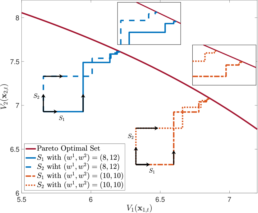
(a) Trajectory of the utility

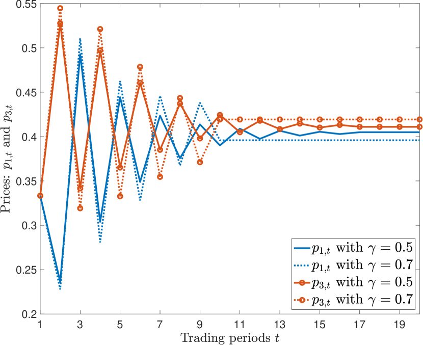
(b) Trajectory of the price

Table 1. Limiting wealth allocation and price in Example 5.2

Wealth		Risk		Limiting Price
$w^{1}$	$w^{2}$	$\gamma$		$p_{1}^{*}$	$p_{2}^{*}$	$p_{3}^{*}$
10	10	0.5 (0.7)	$\mathcal{S}_{1}:$	0.4044 (0.3959)	0.1839 (0.1849)	0.4117 (0.4192)
			$\mathcal{S}_{2}:$	0.4045 (0.4004)	0.1838 (0.1841)	0.4117 (0.4155)
8	12	0.5 (0.7)	$\mathcal{S}_{1}:$	0.4436 (0.4449)	0.1745 (0.1726)	0.3819 (0.3825)
			$\mathcal{S}_{2}:$	0.4440 (0.4800)	0.1743 (0.1741)	0.3817 (0.3459)
12	8	0.5 (0.7)	$\mathcal{S}_{1}:$	0.3624 (0.3463)	0.1933 (0.1959)	0.4443 (0.4578)
			$\mathcal{S}_{2}:$	0.3621 (0.3776)	0.1933 (0.2044)	0.4446 (0.4180)

As demonstrated in Example 5.2, the trading sequence can impact the limiting price. A key observation for understanding this phenomenon is that $\mathcal{S}_{1}$ can be equivalently viewed as $\mathcal{S}_{2}$ preceded by an extra Trader 1 action. Such an action results in an initial market state different from that of the original $\mathcal{S}_{2}$. As Proposition 5.1 suggests, different initial wealth results in a different limiting price; thus the limiting prices for the two sequences $\mathcal{S}_{1}$ and $\mathcal{S}_{2}$ are different. To illustrate, we consider Example 5.2 with $w^{1}=w^{2}=10$. The extra action of $\mathcal{S}_{1}$ (the first trade) yields market states $\mathbf{x}_{1}=(7.49,7.49.13.50)$, $\mathbf{x}_{2}=(10,10,10)$, and $\mathbf{y}=(7.51,7.51,1.50)$. After the first trade, sequence $\mathcal{S}_{1}$ becomes identical to $\mathcal{S}_{2}$. However, for $\mathcal{S}_{2}$, the initial condition is $\mathbf{x}_{1}=(10,10,10)$, $\mathbf{x}_{2}=(10,10,10)$, and $\mathbf{y}=(5,5,5)$, which is different from the states yield from $\mathcal{S}_{1}$ after the first trading, thus the two sequences result in different limiting prices.

Practically, traders interact with the market maker randomly, leading to a random trading path. Consequently, the limiting price becomes a trading-sequence-dependent random variable. However, our next result characterizes the limiting price for a given trading sequence and demonstrates that price invariance can be achieved when the trader population is large.

Theorem 5.3.

For the CRRA-utility-based market, we have the following results:
(i) Given a trading sequence $\mathcal{S}\in\Phi$, the Trading Process 1 converges to the limiting wealth allocation $\{\mathbf{x}_{j}^{*}\}$ characterized by problem $\mathcal{P}_{\textrm{po}}(\boldsymbol{\nu}^{*})$ with some weights $\boldsymbol{\nu}^{*}=(\nu_{1}^{*},\ldots,\nu_{J}^{*})\in\mathbb{R}^{J}_{+}\setminus\{\mathbf{0}\}$; and the limiting price is given by

(20) $$p_{i}^{*}=\xi^{*}_{i}\Big{/}\sum_{k=1}^{I}\xi_{k}^{*},~{}~{}~{}i=1,\ldots,I,$$

where $\boldsymbol{\xi}^{*}=(\xi_{1}^{*},\ldots,\xi_{I}^{*})$ is the unique solution of the following equations:

(21) $$\xi_{i}^{*} =\Bigg{(}\frac{\sum\limits^{J}_{j=1}(\nu_{j}^{*})^{\frac{1}{1-\gamma}}\cdot\pi_{i,j}^{\frac{1}{1-\gamma}}+(\xi_{i}^{*})^{\frac{\gamma-\gamma_{m}}{(1-\gamma)(1-\gamma_{m})}}\cdot\mathcal{L}(\boldsymbol{\xi}^{*},\boldsymbol{\theta})\cdot W_{0}\cdot\theta_{i}^{\frac{1}{1-\gamma_{m}}}}{w_{0}^{\textrm{all}}}\Bigg{)}^{1-\gamma},~{}~{}i=1,\ldots,I$$

where $\mathcal{L}(\boldsymbol{\xi},\boldsymbol{\theta})\triangleq\left(\sum\limits_{k=1}^{I}\theta_{k}(\theta_{k}/\xi_{k})^{\frac{\gamma_{m}}{1-\gamma_{m}}}\right)^{-\frac{1}{\gamma_{m}}}$.
(ii) In Trading Process 1, if traders’ beliefs $\boldsymbol{\pi}_{j}$ and initial wealth $w_{j,0}$ are independently and identically distributed random variables for $j=1,\ldots,J$; with each trader having an equal probability of trading with the market maker at each trading instance, then the solution $\{\xi_{i}^{*}\}|_{i=1}^{I}$ defined in Eq. (21) and the associated limiting price $\{p_{i}^{*}\}|_{i=1}^{I}$ generated by each trading sample path converge almost surely to a pair of constant vectors as the trader population $J\rightarrow\infty$.

The first result in Theorem 5.3 provides an explicit method for computing the limiting price $\mathbf{p}^{*}$ for a sepecified trading sequence with the associated weighting parameters $\boldsymbol{\nu}^{*}$. It is worth noting that the functional form of the limiting price (20) and (21) remain consistent, as the influence of the trading sequence is solely reflected through the weights $\boldsymbol{\nu}^{*}$. The second result in Theorem 5.3 is an interesting product of the price formula. One can consider it a prediction market analogue of the “Law of Large Numbers”. It implies that in a randomly trading market with a large trader population, the variation of limiting price induced by different trading sequences becomes negligible. This underscores the significance of trader participation in prediction markets, as it not only enhances liquidity but also increases the reliability of limiting prices. Imagine a prediction market that yields predictions (limiting price) that are heavily dependent on the trading sequence. In such a case, one cannot know whether its prediction truly represents the overall beliefs or only happens to be a biased result of a specific trading sequence. Such uncertainty will undermine the interpretability of prices and jeopardize the prediction accuracy.

Theorem 5.3 also provides several potentially useful insights for market maker designing. Combining Eqs. (20) and (21), the limiting price has the following decomposition:

(22) $$p_{i}^{*}=\Bigg{(}\sum_{j=1}^{J}\frac{\left(\frac{\nu_{j}}{\sum_{k=1}^{I}\xi_{k}^{*}}\right)^{\frac{1}{(1-\gamma)}}}{w_{0}^{\textrm{all}}}\left(\pi_{i,j}\right)^{\frac{1}{1-\gamma}}+(p_{i}^{*})^{\frac{\gamma-\gamma_{m}}{(1-\gamma)(1-\gamma_{m})}}\cdot\mathcal{L}(\mathbf{p}^{*},\bm{\theta})\frac{W_{0}}{w_{0}^{\textrm{all}}}\theta_{i}^{\frac{1}{1-\gamma_{m}}}\Bigg{)}^{1-\gamma},\quad i=1,\ldots,I.$$

This decomposition can be explained as follows. First, a smaller initial wealth $W_{0}$ can reduce the market maker’s impact on the limiting price. Second, a market maker with higher risk aversion (smaller $\gamma_{m}$) also diminishes its influence on the limiting price because $(p_{i}^{*})^{\frac{\gamma-\gamma_{m}}{(1-\gamma)(1-\gamma_{m})}}$ is a decreasing function of $\gamma_{m}$ for $p_{i}^{*}\in(0,1)$. Third, the function $\mathcal{L}(\mathbf{p}^{*},\boldsymbol{\theta})$ exhibits an intriguing suppressive effect designed to mitigate the price distortion caused by the market maker’ externality. To explain further, $\mathcal{L}(\mathbf{p}^{*},\boldsymbol{\theta})$ reaches its maximum value of $1$ when $\mathbf{p}^{*}=\boldsymbol{\theta}$. When the market consensus $\mathbf{p}^{*}$ significantly deviates from the market maker’s belief $\boldsymbol{\theta}$, the term $\mathcal{L}(\mathbf{p}^{*},\boldsymbol{\theta})$ lessens its impact, effectively reducing the market maker’s influence on the limiting price. It is worth noting that such a suppressive effect stems from the utility preserving condition (8), underscoring the additional benefits of the MU-based mechanism.

With the above results, in the next section, we investigate how to approximate the limiting price under a finite trader scenario through choosing an appropriate weight $\boldsymbol{\nu}^{*}$.

5.2. Heuristic Weighting Parameters and Price Formula

The previous section has emphasized the vital role of determining the weighting parameters, $\boldsymbol{\nu}^{*}$, in solving problem $\mathcal{P}_{\textrm{po}}(\boldsymbol{\nu}^{*})$ to establish the limiting price. Given the practical difficulty of obtaining the “true” weighting parameters $\boldsymbol{\nu}^{*}$ before trading converges, we propose an approximation using deterministic weights. Drawing inspiration from previous analysis, which highlights Pareto optimality of the limiting wealth allocation and underscores the significance of both the initial wealth distribution $w_{j,0}$ and the risk parameter $\gamma$ in shaping the limiting price (e.g., see Table 1), we introduce the concept of Pareto Optimal Induced (POI) weights, denoted as $\hat{\boldsymbol{\nu}}=(\hat{\nu}_{1},\ldots,\hat{\nu}_{J})$ defined as:

(23) $$\hat{\nu}_{j}=\big{(}w_{j,0}\big{)}^{1-\gamma},~{}~{}j=1,\ldots,J.$$

Applying Theorem 5.3, we replace $\boldsymbol{\nu}^{*}$ with the POI weights $\hat{\boldsymbol{\nu}}$ in Eq. (21) to calculate the associated POI limiting price, denoted as $\hat{\mathbf{p}}=(\hat{p}_{1},\ldots,\hat{p}_{I})$, with its components given as follows:

(24) $$\hat{p}_{i}=\hat{\xi}_{i}\Big{/}\sum_{k=1}^{I}\hat{\xi}_{k},~{}~{}~{}i=1,\ldots,I,\$$

where $\hat{\boldsymbol{\xi}}=(\hat{\xi}_{1},\ldots,\hat{\xi}_{I})$ is the unique solution of the following equation,

(25) $$\hat{\xi}_{i}=\Bigg{(}\frac{\sum\limits^{J}_{j=1}w_{j,0}\cdot\pi_{i,j}^{\frac{1}{1-\gamma}}+\hat{\xi}_{i}^{\frac{\gamma-\gamma_{m}}{(1-\gamma)(1-\gamma_{m})}}\cdot\mathcal{L}(\hat{\boldsymbol{\xi}},\boldsymbol{\theta})\cdot W_{0}\cdot\theta_{i}^{\frac{1}{1-\gamma_{m}}}}{w_{0}^{\textrm{all}}}\Bigg{)}^{1-\gamma},~{}~{}i=1,\ldots,I.$$

Now we provide some interpretation for the POI limiting price. Eq (25) implies that the price $\hat{p}_{i}$ is directly linked to a weighted average that considers all participants’ wealth and risk-adjusted beliefs regarding the $i$-th asset. More specifically, the term $\sum\limits_{j=1}^{J}w_{j,0}\cdot\pi_{i,j}^{\frac{1}{1-\gamma}}$ represents the avarage risk-adjusted belief contributed from all the traders weighted by their own wealth. In contrast, the term $\hat{\xi}_{i}^{\frac{\gamma-\gamma_{m}}{(1-\gamma)(1-\gamma_{m})}}\cdot\mathcal{L}(\hat{\boldsymbol{\xi}},\boldsymbol{\theta})\cdot W_{0}\cdot\theta_{i}^{\frac{1}{1-\gamma_{m}}}$ which combines the risk difference and belief divergence, controls the contribution of market maker’s risk-adjusted belief in such a price.

The POI price formula (24) and (25) encompass specific market scenarios as special cases. When both market maker and traders adopt the logarithmic utilities, i.e., $\gamma=\gamma_{m}=0$ in (17), Eq. (25) will simplify to:

(26) $$\hat{\xi}_{i}=\frac{\sum\limits^{J}_{j=1}w_{j,0}\cdot\pi_{i,j}+\mathcal{L}_{0}(\hat{\boldsymbol{\xi}},\boldsymbol{\theta})\cdot W_{0}\cdot\theta_{i}}{w_{0}^{\textrm{all}}},~{}~{}~{}i=1,\ldots,I,$$

where $\mathcal{L}_{0}(\hat{\boldsymbol{\xi}},\boldsymbol{\theta})=\exp(-\sum\limits_{k=1}^{I}\theta_{k}\log(\theta_{k}/\hat{\xi}_{k}))$ representing the exponential Kullback-Leibler Divergence (KLD) between $\boldsymbol{\theta}$ and $\hat{\boldsymbol{\xi}}$. If we further set $\mathcal{L}_{0}(\hat{\boldsymbol{\xi}},\boldsymbol{\theta})\equiv 1$ then the price formula (24) becomes the wealth-weighted average of market beilefs discussed in (Sethi and Vaughan, 2016).

We would like to highlight that the solution methodology for deriving the CRRA-utility based limiting price, e.g., Eq. (21) and the POI weights (23) remain applicable even when market participant’s MU functions extend beyond the CRRA family of utilities. One example is the hybrid market model where the market maker adopts exponential utility, as given by Eq. (10), while the traders adopt logarithmic utility. In this scenario, the POI limiting price remains the same as (24), but the equations for $\hat{\boldsymbol{\xi}}$ become:

(27) $$\hat{\xi}_{i}=\frac{\sum\limits_{j=1}^{J}w_{j,0}\cdot\pi_{i,j}+\frac{1}{\beta}\hat{\xi}_{i}\log\left(\theta_{i}\Big{/}\frac{\hat{\xi}_{i}}{\sum_{k=1}^{I}\hat{\xi}_{k}}\right)}{\sum\limits_{j=1}^{J}w_{j,0}},\quad i=1,2,...,I.$$

We provide more details of Eq. (27) in Appendix A.5. Our numerical experiments (given in Appendix A.5) demonstrate that the price formula (27) outperforms the conventional wealth-weighted average price reported in (Sethi and Vaughan, 2016). The CRRA-utility-based pricing formula can also be extended to a more comprehensive market model where all participants adopt utilities with hyperbolic absolute risk aversion (HARA utility), which finds wide applications in economic modeling. A brief discussion of this model is presented in Appendix A.6.

5.3. Evaluation of Approximation Scheme

In this section, we first employ simulation to validate the accuracy of the POI weights (23) and the price formula (24) in estimating the true weighting coefficients and the true limiting price, respectively. Following this validation, we proceed to examine how the risk parameters and initial wealth impact the accuracy of our approximation.

We consider a CRRA-utility-based market with $I=3$, $W_{0}=10$, and $\theta_{1}=\theta_{2}=\theta_{3}=1/3$. Traders are generated randomly as follows. The $j$-th trader’s belief is sampled from $\boldsymbol{\pi}_{j}=\alpha\cdot\bar{\boldsymbol{\pi}}+(1-\alpha)\cdot\boldsymbol{\epsilon}/|\boldsymbol{\epsilon}|$, where $\bar{\boldsymbol{\pi}}$ is the baseline belief evenly sampled from $(0.6,0.2,0.2)$ and $(0.2,0.2,0.6)$; $\boldsymbol{\epsilon}$ is uniformly distributed random noise on $[0,1]^{3}$, and $\alpha=0.5$ controls the market belief structure. We conduct simulations according to Trading Process 1, with each trader randomly selected with equal probability to interact with the market maker at each time period. For each set of parameters, we perform $N=5\times J$ rounds of simulation, and we denote the $k$-th sample of the limiting wealth allocation as $\{\mathbf{x}_{1}^{\textrm{sim}}(k),\ldots,\mathbf{x}_{J}^{\textrm{sim}}(k)\}|_{k=1}^{N}$.

• Evaluation by limiting wealth: To verify the accuracy of the POI weights (23), we first solve the problem $\mathcal{P}_{\textrm{po}}(\hat{\boldsymbol{\nu}})$ whose solution is denoted as $\{\hat{\mathbf{x}}_{1},\ldots,\hat{\mathbf{x}}_{J}\}$. If the heuristic weight $\hat{\boldsymbol{\nu}}$ provides an accurate approximation for the “true” weighting parameter, then the wealth allocation $\{\hat{\mathbf{x}}_{1},\ldots,\hat{\mathbf{x}}_{J}\}$ should be close to the sample limiting wealth allocation $\{\mathbf{x}_{1}^{\textrm{sim}}(k),\ldots,\mathbf{x}_{J}^{\textrm{sim}}(k)\}|_{k=1}^{N}$ generated by the simulation. We introduce the following quantity to measure the difference for each sample,

  $$\delta_{\mathbf{x}}(k)\triangleq\sum\limits_{j=1}^{J}\|\mathbf{x}_{j}^{\textrm{sim}}(k)-\hat{\mathbf{x}}_{j}\|\big{/}\sum\limits_{j=1}^{J}\|\mathbf{x}_{j}^{\textrm{sim}}(k)\|,$$

  for $k=1,\ldots,N$. The sample mean and variance of $\delta_{\mathbf{x}}(k)$ is denoted by $\textrm{E}[\delta_{\mathbf{x}}]$ and $\textrm{Var}[\delta_{\mathbf{x}}]$, respectively.

• Evaluation by limiting price: We denote the price associated with the $k$-th sample of limting wealth as $\mathbf{p}^{\textrm{sim}}(k)$ and we compute the POI price $\hat{\mathbf{p}}$ by using (24). To measure the difference between these prices, we employ the Kullback-Leibler Divergence (KLD), i.e., given two prices $\mathbf{p}^{a},\mathbf{p}^{b}\in\Delta_{I}$, the KLD of these prices is defined as $\mathcal{D}(\mathbf{p}^{a},\mathbf{p}^{b})\triangleq\sum_{i=1}^{I}p^{a}_{i}\ln\left(p^{a}_{i}/p^{b}_{i}\right)$. We then denote the KLD between the $k$-th sample price $\mathbf{p}^{\textrm{sim}}(k)$ and the POI price $\hat{\mathbf{p}}$ as $\delta_{\mathbf{p}}(k)\triangleq\mathcal{D}(\mathbf{p}^{\textrm{sim}}(k),\hat{\mathbf{p}})$ for $k=1,\ldots,N$. We then compute the sample mean and sample variance of $\delta_{\mathbf{p}}(k)$ as $\text{E}[\delta_{\mathbf{p}}]$ and $\textrm{Var}[\delta_{\mathbf{p}}]$, respectively.

Table 2 reports the comparative results for different setups ($\gamma_{m},\gamma\in\{-2,0.5\}$ and $J\in\{50,100,200,400\}$). For each set of risk parameters, denoted as ($\gamma_{m}$, $\gamma$), we list the results for different values of $J$. The results clearly show that, regardless of the different settings, the POI weights (23) and the POI price (24) perform exceptionally well, exhibiting minimal disparities in both wealth and price. A closer examination reveals several noteworthy patterns. Firstly, for a fixed set of risk parameters $\gamma_{m}$ and $\gamma$, increasing the trader population $J$ enhances the accuracy of our approximation. This enhancement is evident as all error and variation indicators decrease with the increase in $J$. Of particular significance is the observation that Table 2 also highlights a notable decrease in approximation variances, $\textrm{Var}[\delta_{\mathbf{x}}]$ and $\textrm{Var}[\delta_{\mathbf{p}}]$, with a larger population. This reduction in variance can be attributed to the decrease in variation stemming from the trading sequence. Consequently, this pattern confirms the second result outlined in Theorem 5.3, which posits that a larger population leads to a more stable limit price. Secondly, for a given trader population, the approximation error is smaller in scenarios with $\gamma_{m}=-2$ compared to those with $\gamma_{m}=0.5$, suggesting that our approximation is more favorable for higher levels of risk aversion.

Table 2. Verification of approximation scheme

Market Par.			Price Diff.		Wealth Diff.
$\gamma_{m}$	$\gamma$	$J$	$\textrm{E}[\delta_{\mathbf{p}}]$	$\textrm{Var}[\delta_{\mathbf{p}}]$	$\textrm{E}[\delta_{\mathbf{x}}]$	$\textrm{Var}[\delta_{\mathbf{x}}]$
-2	-2	50	$1.71\text{\times}{10}^{-05}$	$5.75\text{\times}{10}^{-10}$	$5.75\text{\times}{10}^{-04}$	$9.30\text{\times}{10}^{-08}$
-2	-2	100	$8.84\text{\times}{10}^{-06}$	$2.61\text{\times}{10}^{-10}$	$2.48\text{\times}{10}^{-04}$	$1.76\text{\times}{10}^{-08}$
-2	-2	200	$2.54\text{\times}{10}^{-06}$	$1.35\text{\times}{10}^{-11}$	$1.84\text{\times}{10}^{-04}$	$1.31\text{\times}{10}^{-08}$
-2	-2	400	$1.51\text{\times}{10}^{-06}$	$4.52\text{\times}{10}^{-12}$	$1.26\text{\times}{10}^{-04}$	$6.06\text{\times}{10}^{-09}$
-2	0.5	50	$1.04\text{\times}{10}^{-04}$	$1.35\text{\times}{10}^{-08}$	$9.69\text{\times}{10}^{-04}$	$2.31\text{\times}{10}^{-07}$
-2	0.5	100	$4.33\text{\times}{10}^{-05}$	$1.75\text{\times}{10}^{-09}$	$4.29\text{\times}{10}^{-04}$	$4.10\text{\times}{10}^{-08}$
-2	0.5	200	$3.20\text{\times}{10}^{-05}$	$1.17\text{\times}{10}^{-09}$	$2.50\text{\times}{10}^{-04}$	$1.79\text{\times}{10}^{-08}$
-2	0.5	400	$1.91\text{\times}{10}^{-05}$	$5.48\text{\times}{10}^{-10}$	$1.35\text{\times}{10}^{-04}$	$6.37\text{\times}{10}^{-09}$
0.5	-2	50	$5.08\text{\times}{10}^{-05}$	$3.60\text{\times}{10}^{-08}$	$2.77\text{\times}{10}^{-03}$	$6.64\text{\times}{10}^{-06}$
0.5	-2	100	$1.84\text{\times}{10}^{-05}$	$1.78\text{\times}{10}^{-08}$	$9.70\text{\times}{10}^{-04}$	$1.42\text{\times}{10}^{-06}$
0.5	-2	200	$5.34\text{\times}{10}^{-06}$	$2.00\text{\times}{10}^{-10}$	$5.09\text{\times}{10}^{-04}$	$2.45\text{\times}{10}^{-07}$
0.5	-2	400	$2.01\text{\times}{10}^{-06}$	$7.94\text{\times}{10}^{-11}$	$3.66\text{\times}{10}^{-04}$	$8.11\text{\times}{10}^{-08}$
0.5	0.5	50	$3.83\text{\times}{10}^{-05}$	$1.20\text{\times}{10}^{-09}$	$2.89\text{\times}{10}^{-03}$	$2.03\text{\times}{10}^{-06}$
0.5	0.5	100	$1.95\text{\times}{10}^{-05}$	$2.23\text{\times}{10}^{-10}$	$1.34\text{\times}{10}^{-03}$	$3.24\text{\times}{10}^{-07}$
0.5	0.5	200	$8.61\text{\times}{10}^{-06}$	$3.38\text{\times}{10}^{-11}$	$6.70\text{\times}{10}^{-04}$	$6.12\text{\times}{10}^{-08}$
0.5	0.5	400	$2.15\text{\times}{10}^{-06}$	$3.47\text{\times}{10}^{-12}$	$3.18\text{\times}{10}^{-04}$	$1.77\text{\times}{10}^{-08}$

We proceed to examine how the risk parameters and initial wealth affect the quality of our approximation. To better illustrate the impact of these parameters, we introduce the conventional wealth-weighted price formula from (Sethi and Vaughan, 2016) as a benchmark, denoted as $\breve{\mathbf{p}}=(\breve{p}_{1},\ldots,\breve{p}_{I})$, where

(28) $$\breve{p}_{i}=\frac{\theta_{i}\cdot W_{0}+\sum\limits_{j=1}^{J}w_{j,0}\pi_{i,j}}{W_{0}+\sum\limits_{j=1}^{J}w_{j,0}},~{}~{}i=1,\ldots,I.$$

We follow a simulation procedure similar to that in Table 2, using a fixed $J=50$ and $\gamma_{m}=-0.5$. To highlight the impact of traders’ risk parameter $\gamma$, we vary its values and compare the resulting limiting prices obtained from the simulation with two heuristic price formulas: (24) and (28).

Figure 2. Comparison of two heuristics for different risk parameters

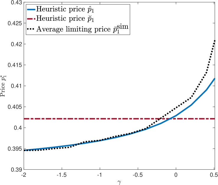
(a) Price $p_{1}^{*}$ and $\gamma$

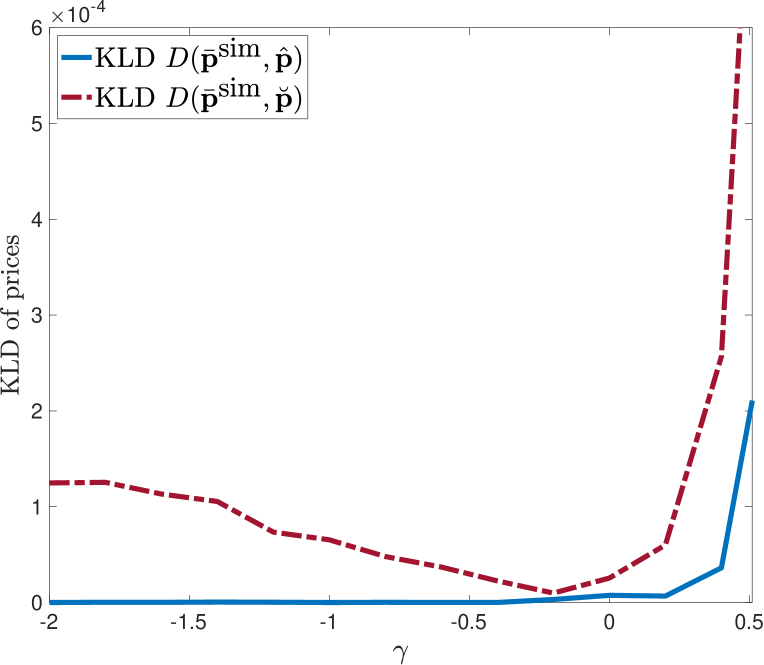
(b) KLD and $\gamma$

In Figure 2(a), the red curve represents the average price of the first security resulting from $N=250$ rounds of simulations, which exhibits an increasing trend as $\gamma$ increases. Importantly, our POI price formula (24) effectively captures this trend, as indicated by the solid blue curve. In contrast, the conventional wealth-weighted formula (28) fails to exhibit such a distinct pattern as it does not account for the risk parameter. Figure 2(b) illustrates the approximation errors of the two heuristic prices where $\mathcal{D}(\bar{\mathbf{p}}^{\textrm{sim}},\hat{\mathbf{p}})$ and $\mathcal{D}(\bar{\mathbf{p}}^{\textrm{sim}},\breve{\mathbf{p}})$ measure the KLD between the simulated average price and the two heuristic prices, respectively. Notably, when $\gamma$ deviates from $0$, especially when it is below zero, our price formula (24) significantly outperforms the conventional wealth-weighted formula (28).

Figure 3. Comparison of two heuristics for different initial wealth

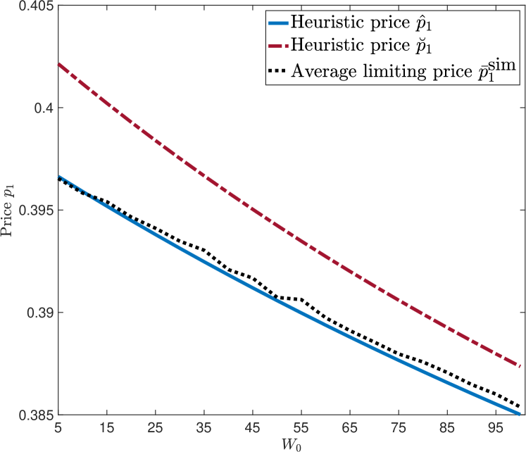
(a) Price and market maker’s wealth

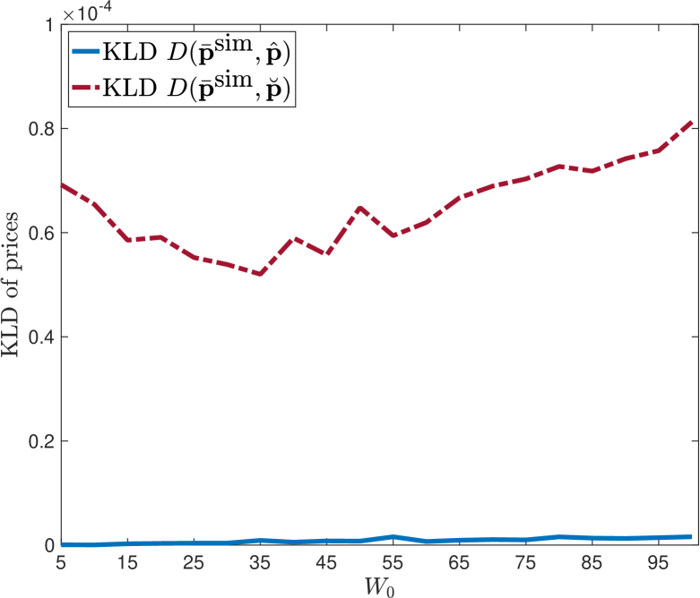
(b) KLD and market maker’s wealth

We then investigate the impact of the market maker’s initial wealth $W_{0}$, which is a key design variable for providing liquidity. Holding $\gamma_{m}=\gamma=-2$, we incrementally raise $W_{0}$ from $5$ to $100$. In Figure 3(a), the limiting price decreases as $W_{0}$ increases. This is because the price becomes increasingly biased towards the market maker’s own belief (i.e., $\theta_{i}=1/3$) as its wealth grows. Both formulas (24) and (28) display a similar trend. However, our price formula (24) closely tracks the limiting price, while the conventional one (28) tends to overestimate it significantly. Figure 3(b) provides a more detailed comparison of these approximation errors by evaluating the KLD. It becomes evident that our POI price formula (24) not only demonstrates greater accuracy but also exhibits much higher stability than formula (28) when varying the market maker’s wealth $W_{0}$. This characteristic highlights that the quality of our heuristic price formula (24) is not sensitive to fluctuations in the market maker’s wealth level. Such a property may benefit the market maker in customizing the market-making mechanism.

In summary, the combination of the POI weights (23) with Eq. (21) offers an accurate estimation of the limiting price across various market scenarios. Although such a pricing formula is not entirely analytical, the parameters $\xi_{i}^{*}$, given in Eqs. (21) provide comprehensive information on how the price is aggregated based on participants’ beliefs, risk attitudes, and wealth levels.

6. Price-Volume Relationship and Nonstationary Market

In this section, we provide analysis of the price-volume relationship resulted from our model and discuss the market behavior in a non-stationary market.

The price-volume relationship: Like microstructure analysis in the financial market, studying the relationship between the price and trading volume reveals how prices evolve during trading. To examine this, we consider the $t$-th round of trading where the $j$-th trader interacts with the market maker in Trading Process 1. Although it might seem like only one trader is trading at a time, we can think of this as a group of traders. For instance, the $j$-th trader represents a group of traders holding the similar beliefs with the wealth being the aggregate wealth. Therefore, the order size in each round of trading represents an aggregate order for a group of traders. For simplicity, we consider a market with binary securities ($I=2$). The $j$-th trader solves problem $\mathcal{P}_{j}(\mathbf{x}_{j,t})$ to determine the optimal decision $\mathbf{z}^{*}=(z_{1}^{*},z_{2}^{*})$. Since the two securities are mutually exclusive, the trading volume is only related to the net demand $\textrm{D}_{t}\triangleq\Delta q_{1}^{*}-\Delta q_{2}^{*}=z^{*}_{1}-z^{*}_{2}$ where $q_{i}^{*}$ is the amount of the order. The mutual exclusiveness also implies the prices $\mathbf{p}_{t}=(p_{1,t},p_{2,t})$ satisfies $p_{1,t}=1-p_{2,t}$. We then examine the relationship between the net demand $\text{D}_{t}$ and the security’s price $p_{1,t}$ for different market settings.

As the exponential MU-function-based market admits a closed-form solution for trading problem $\mathcal{P}_{j}(\mathbf{x}_{j})$, it is an ideal vehicle to study the price-volume relationship. Using the expression (11) in Proposition 4.1, we can compute the net demand as,

(29) $$\textrm{D}_{t}=z^{*}_{1}-z^{*}_{2} =\frac{1}{\alpha_{j}+\beta}\ln\left(\frac{\hat{\pi}_{1,j,t}(1-p_{1,t})}{(1-\hat{\pi}_{1,j,t})p_{1,t}}\right)=\frac{1}{\alpha_{j}+\beta}\left(\ln\left(\frac{\hat{\pi}_{1,j,t}}{1-\hat{\pi}_{1,j,t}}\right)-\ln\left(\frac{p_{1,t}}{1-p_{1,t}}\right)\right),$$

where $\hat{\pi}_{i,j,t}$ is defined in Proposition 4.1. We observe that the volume $\textrm{D}_{t}$ is proportional to the difference between the log odds of the $j$-th trader’s belief and the security price. The demand $\text{D}_{t}$ decreases as the price $p_{1,t}$ increases, indicating a higher demand for the security at a lower price. Conversely, for a fixed price $p_{1,t}$, the demand $\text{D}_{t}$ depends on the trader’s utility-adjusted belief $\hat{\pi}_{1,j,t}$. A trader trades more security if $\hat{\pi}_{1,j,t}$ deviates further from the price. It is also evident that the net trade volume is discounted by a factor $\frac{1}{\alpha_{j}+\beta}$. That is to say, even if two traders have identical subjective beliefs, the trader who is more risk-averse trades less security than the one with less risk aversion. This finding further demonstrates the importance of including the risk parameter in our approximated pricing formula (25).

The above price-volume relationship also holds for the CRRA utility-based market. We slightly modify the market in Example 5.2 by aggregating the first two securities as a single security, which gives a binary market. That is, the two traders’ beliefs become $\pi_{1}=(0.4,0.6)$ and $\pi_{2}=(0.7,0.3)$. Figure 4 plots trader 2’s net demand as a function of $p_{1,t}$ for diffferent paramters, i.e., $\gamma_{m},\gamma\in\{0.5,-0.5\}$ and $W_{0}\in\{5,10\}$. Clearly, we can observe the pattern that the net demand is negatively correlated with the price and the risk aversion parameter. In addition, this figure also indicates that when the market maker has larger wealth, it may provide higher trading volume (higher liquidity).

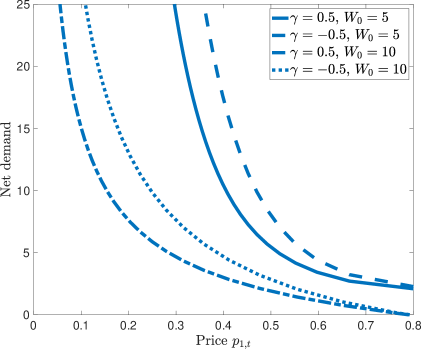
Figure 4. Demand as function of price for CRRA utility

Nonstationary market: All the previous analysis is based on the stationary assumption, i.e., we assume that no new information comes to the market during trading. However, in reality, most prediction markets run for several months, and when an event shocks the market, traders’ beliefs are significantly changed. To show how new information affects security prices, we consider two situations: the shock happens at an early stage (before price convergence), and the shock happens at a late stage. We adopt Example 5.2 for illustration. The shock changes the traders’ beliefs on the second security, i.e., the original beliefs, $\pi_{1}=(0.2,0.2,06)$ and $\pi_{2}=(0.6,0.1,0.3)$ are modified to $\hat{\pi}_{1}=\text{normalize}\{(0.2,0.2,0.6)+(0,1,0)\}=(0.1,0.6,0.3)$ and $\hat{\pi}_{2}=\text{normalize}\{(0.6,0.1,0.3)+(0,1,0)\}=(0.3,0.55,0.15)$, respectively. Figure 5(a) displays the trajectories of two traders’ utilities. The solid line and dash-dot line indicate the Pareto optimal frontiers of utility values generated by the original and modified beliefs, respectively. We can observe that, regardless of when the shock occurs, the utilities ultimately converge to the new Pareto-optimal set (i.e., the solid curve and the dashed curve indicate the Pareto-optimal sets for the market with and without the shock, respectively). However, the position of the limiting points varies. Figure 5(b) illustrates the trajectory of the first security’s price, $p_{1,t}$. Similar to the utility values, when new information enters the market, the price $p_{1,t}$ responds rapidly to this new information. It is important to note that the limiting prices resulting from early and late shocks are different. This is a straightforward consequence of Theorem 5.3, which indicates that all traders’ initial conditions and beliefs determine the limiting price. If we consider the time at which the shock occurs as the new starting point, early and late shocks produce different initial conditions, thus potentially leading to different limiting prices.

Figure 5. Utility and price trajectories after shock

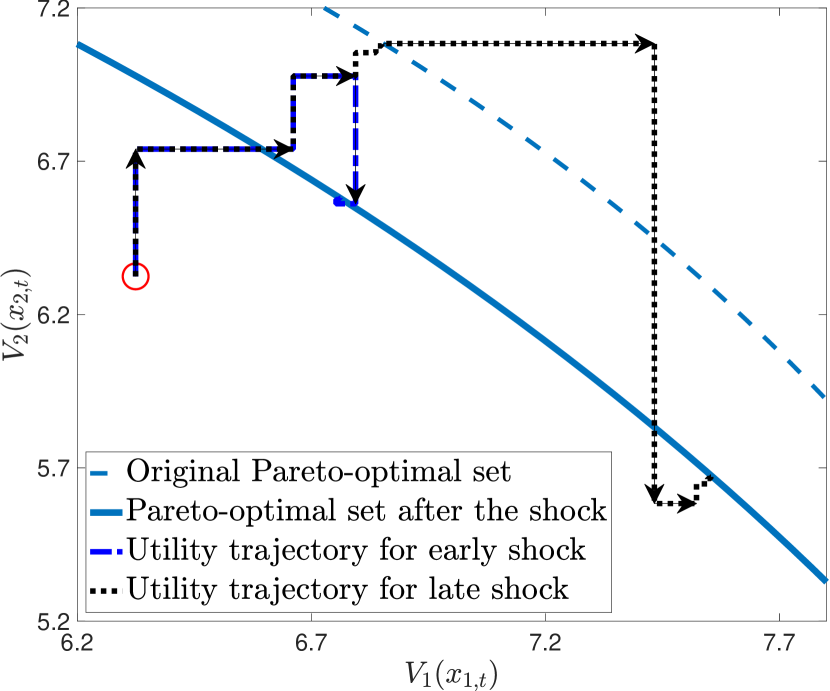
(a) Utility trajectories

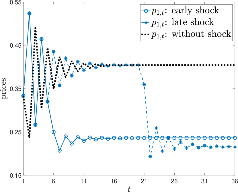
(b) Price trajectories

7. Conclusion

This paper studies the prediction market convergence properties through the utilization of the multivariate utility (MU)-based market-making mechanism. This mechanism not only consolidates various existing market-making methods under specific conditions but also establishes a framework for examining the dynamic trading process within a market featuring a single market maker and a finite number of traders. Within this framework, we address one fundamental question arising in the prediction market: the formation of the limiting price (final price) by all market participants. We establish, under mild conditions, that traders’ wealth processes converge to a limiting wealth distribution, resulting in Pareto optimal utility levels for all participants. This outcome enables us to explore the limiting price across different market types. In exponential utility markets, we present an explicit formula for the limiting price. For convex risk-measure-based markets, we introduce a method to design MU functions via penalty functions and demonstrate that the limiting price is uniquely determined as a weighted power mean of trader beliefs. Regarding CRRA utility-based markets, we characterize the limiting price through a system of equations. Additionally, we present a theoretical result indicating that the impact of trading sequence variation becomes negligible as the trader population increases. This novel finding enables us to formulate an approximate price formula, suggesting that the limiting price can be construed as a wealth-weighted risk-adjusted average of all participants’ beliefs. Numerical experiments validate the high accuracy and robustness of this approximation.

There are several promising directions for future research. Firstly, although this work has derived price formulas under various theoretical settings, a critical next step is the empirical validation of these results using real market data.

Secondly, our model is built on the stationary assumption that participants’ beliefs remain constant. In real-world trading, traders and market maker typically adaptively revise their beliefs based on new information. While our preliminary analysis in Section 6 indicates that changes in traders’ beliefs can result in significant shifts in the limiting price, it remains unknown how traders and market maker should incorporate this new information into their decision-making process as part of a learning process. A recent study by (Birge et al., 2021) analyzes the profit maximization problem for market maker in the spread betting market, where market maker may learn the distribution of event outcomes during trading. To address the potential profit loss that Bayesian policies may suffer in the presence of strategic bettors, they propose a new policy that balances learning with bluff-proofing. Building on this line of research, our model has the potential to incorporate learning features for both traders and market maker.

Thirdly, in our model, we assume that traders’ decision problems are myopic, meaning that they focus on single-period decision problems. However, in the actual market, some traders exhibit forward-looking behavior. For example, some professional traders may possess significant insights into future market movements. Therefore, it is worthwhile to explore a model that incorporates traders who tackle forward-looking decision problems involving multi-period considerations. In such a scenario, the decision horizon spans multiple periods, which introduces more price uncertainty resulting from the trading activities of other market participants. Establishing a tractable multi-period decision problem for traders is a crucial step in exploring this forward-looking aspect in the market.

Lastly, it is well-known that classical risk-averse preferences cannot fully explain certain decision-making behaviors observed in empirical studies and psychological experiments (Tversky and Kahneman, 1992). Prospect theory (PT) is an influential alternative theory that accounts for psychological factors such as loss aversion, reference points, and probability distortion in individual decision-making ((Kahneman and Tversky, 2013; Barberis, 2013)). Recently, (Yu et al., 2022) adopt a PT-based utility and construct an equilibrium model to explain pricing anomalies in betting markets. In the context of pricing models, (den Boer and Keskin, 2022) incorporate the PT-based demand function into a dynamic pricing model with demand learning and propose an asymptotically optimal dynamic pricing policy. Incorporating PT-based traders into the current analysis could provide a more realistic representation of real-world trading. Furthermore, it would be intriguing to explore how such traders influence the limiting price. However, establishing market convergence could be challenging due to the non-convex nature of the PT-based model. To address this challenge, several key assumptions made in this work may require refinement.

Appendix A Proof of Main Results for Market Convergence Analysis

A.1. Proofs of Main Results in Section 2

The proof of Proposition 2.1 is provided in B.2. We begin with Proposition 2.2.

$\bullet$ Proof of Proposition 2.2:

Proof.

Given states $w_{j,t}$, $\mathbf{q}_{j,t}$, $W_{t}$ and $\Delta\mathbf{q}$, we introduce functions $h_{U}(\cdot):\mathbb{R}\rightarrow\mathbb{R}$ as $h_{U}(w)=U((W_{t}+w)\cdot\mathbf{e}-(Q_{t}+\Delta\mathbf{q}))$ and $h_{V}(\cdot):\mathbb{R}\rightarrow\mathbb{R}$ as $h_{V}(w)=V_{j}((w_{j,t}-w)\cdot\mathbf{e}+(\mathbf{q}_{j,t}+\Delta\mathbf{q}))$ for some $w\in\mathbb{R}$. Assumption 1 implies that $h_{U}(\cdot)$ is a strictly increasing and concave function. Now we consider the two level optimization problem $\bar{\mathcal{P}}_{j}(w_{j,t},\mathbf{q}_{j,t})$. In lower-level problem (3), the constraint $h_{U}(w)\geq U(W_{0}\cdot\mathbf{e})$ actually defines a feasible interval of $w$, e.g., $w\in[h_{U}^{-1}(U(W_{0}\mathbf{e})),\infty)$ where $h_{U}^{-1}(\cdot)$ is the inverse function of $h_{U}(\cdot)$. On the other hand, Assumption 2 implies that $h_{V}(w)$ is a strictly decreasing function of $w$. Based on these properties, when $\Delta\mathbf{q}$ is fixed, replacing the objective function “$\min_{w}~{}w$” by “$\max_{w}~{}h_{V}(w)$” in the lower-level problem defined in constraint (3) does not change its optimal solution for $\Delta w$. After the replacement, the subproblem can be viewed as a partial optimization of the master problem for a given $\Delta\mathbf{q}$, therefore, it can be viewed as the following problem which optimizes $\Delta w$ and $\Delta\mathbf{q}$ simultaneously,

$$\max_{\Delta w\in\mathbb{R},\Delta\mathbf{q}\in\mathbb{R}^{I}}~{} ~{}V_{j}((w_{j,t}-\Delta w)\cdot\mathbf{e}+(\mathbf{q}_{j,t}+\Delta\mathbf{q}))$$

subject to $$~{}U\big{(}(W_{t}+\Delta w)\cdot\mathbf{e}-(\mathbf{Q}_{t}+\Delta\mathbf{q})\big{)}\geq U(W_{0}\mathbf{e}),$$

$$~{}(W_{t}+\Delta w)\cdot\mathbf{e}-(\mathbf{Q}_{t}+\Delta\mathbf{q})\in\textbf{{dom}}(U),$$

$$~{}(w_{j,t}-\Delta w)\cdot\mathbf{e}+(\mathbf{q}_{j,t}+\Delta\mathbf{q})\in\textbf{{dom}}(V_{j}).$$

Letting $\mathbf{x}_{j,t}=w_{j,t}\cdot\mathbf{e}+\mathbf{q}_{j,t}$, $\mathbf{y}_{t}=W_{t}\cdot\mathbf{e}-\mathbf{Q}_{t}$ and $\mathbf{z}=\Delta\mathbf{q}-\Delta w\cdot\mathbf{e}$ in above problem gives problem $\mathcal{P}_{j}(\mathbf{x}_{j,t})$. The uniqueness of the solution follows from the strict concavity of $V_{j}(\cdot)$. $\square$

$\bullet$ Proof of Proposition 2.3:

Proof.

We first prove the proposition under condition (i). Given the market maker’s wealth level $W$ and asset position (where we ignore the subscript $t$), we denote the neighborhood of $\mathbf{Q}$ as $\mathbb{B}(\mathbf{Q};r)=\{\mathbf{a}\in\mathbb{R}^{I}~{}|~{}\|\mathbf{a}-\mathbf{Q}\|\leq r\}$ for some $r>0$. First, we show that, if $\mathbf{y}=W\cdot\mathbf{e}-\mathbf{Q}$ is an interior point of $\textbf{{dom}}(U)$ and $U(\mathbf{y})=U(W_{0}\cdot\mathbf{e})$, then there exists some $r>0$ such that, any order $\Delta\mathbf{q}$ satisfying $\mathbf{Q}+\Delta\mathbf{q}\in\mathbb{B}(\mathbf{Q};r)$ can be priced by solving the following equation,

(30) $$U((W+\Delta w)\cdot\mathbf{e}-(\mathbf{Q}+\Delta\mathbf{q}))=U(\mathbf{y}+\Delta w\cdot\mathbf{e}-\Delta\mathbf{q})=U(W_{0}\cdot\mathbf{e}),$$

where $\Delta w$ is the price of the order $\Delta\mathbf{q}$. Indeed, let $2r>0$ be any number that is less than the minimal distance between $\mathbf{y}$ and boundary of $\textbf{{dom}}(U)$. Then $\mathbf{y}-\Delta\mathbf{q}$ will be an interior point of $\textbf{{dom}}(U)$ for any order $\|\Delta\mathbf{q}\|\leq r$. If $U(\mathbf{y}-\Delta\mathbf{q}))$$<$$U(W_{0}\mathbf{e})$, then the monotonicity and continuity of $U(\cdot)$ imply that there exists a $\Delta w$ satisfies Eq.(30). Thus, the quantity $\Delta w$ solves the pricing problem $\mathcal{P}_{\textrm{cmin}}(\Delta\mathbf{q})$ and it is indeed the price of order $\Delta\mathbf{q}$. On the other hand, if $U(\mathbf{y}-\Delta\mathbf{q})>U(W_{0}\cdot\mathbf{e})$, since $\|\Delta\mathbf{q}\|\leq r$, it has $-r\cdot\mathbf{e}-\Delta\mathbf{q}\leq\mathbf{0}$. The monotonicity of $U(\cdot)$ implies $U(\mathbf{y}-r\mathbf{e}-\Delta\mathbf{q})$$\leq$$U(\mathbf{y})=U(W_{0}\cdot\mathbf{e})$. Thus, there exists a $\Delta w\in[-r,0)$ such that Eq. (30) holds due to continuity and monotonicity of $U(\cdot)$. The above result means that for any small order $\Delta\tilde{\mathbf{q}}$ satisfying $\mathbf{Q}+\Delta\tilde{\mathbf{q}}\in\mathbb{B}(\mathbf{Q};r)$, its price $\Delta\tilde{w}$ can be determined by Eq. (30). Now, we consider small order $\epsilon\cdot\mathbf{e}_{i}$ satisfying $\mathbf{Q}+\epsilon\cdot\mathbf{e}_{i}\in\mathbb{B}(\mathbf{Q};r)$. The price $\Delta w^{i}$ of the order $\epsilon\mathbf{e}_{i}$ is the solution of the equation

(31) $$U(\mathbf{y}+\Delta w_{i}\cdot\mathbf{e}-\epsilon\cdot\mathbf{e}_{i})~{}=~{}U(W_{0}\cdot\mathbf{e}).$$

Recall that the instantaneous price of $i$-th security is the unit cost of purchasing an infinitesimal $\epsilon\mathbf{e}_{i}$, i.e., it is $p_{i}=\frac{d\Delta w^{i}}{d\epsilon}=\lim_{\epsilon\rightarrow 0}\frac{\Delta w^{i}}{\epsilon}$. We apply implicit differentiation rule with respect to $\epsilon$ on equation (31), which gives,

(32) $$-\frac{\partial U}{\partial y^{i}}+\frac{d\Delta w^{i}}{d\epsilon}\sum_{k=1}^{I}\frac{\partial U}{\partial y^{k}}\frac{\partial y^{k}}{\partial\Delta w^{i}}=0~{}\implies~{}~{}p^{i}=\lim_{\epsilon\rightarrow 0}\frac{d\Delta w^{i}}{d\epsilon}=\frac{\frac{\partial U}{\partial y^{i}}}{\sum\limits_{k=1}^{I}\frac{\partial U}{\partial y^{k}}}.$$

Note that the conditions (ii) in Proposition 2.3 just ensure that $\mathbf{y}$ to be an interior in $\textbf{{dom}}(U)$. Thus, the proof for this condition is similar to condition (i). $\square$

A.2. Proof of Theorem 3.2

Before we prove Theorem 3.2, we need the following result.

Lemma A.1.

Under Assumptions 1 and 2, the feasible market states set $\mathcal{A}$ is a compact set.

Proof.

The set $\mathcal{A}$ is closed as it results from the intersection of closed sets, and it’s convex due to the convex nature of $U(\cdot)$ and $V_{j}(\cdot)$. To prove the compactness, we only need to demonstrate that $\mathcal{A}$ is bounded. Suppose $\mathcal{A}$ is unbounded, which implies the existence of a recession direction $(\mathbf{d}_{1},\mathbf{d}_{2},\ldots,\mathbf{d}_{J})$ such that $\mathbf{d}_{j^{\prime}}\neq 0$ for some $j^{\prime}$. This means that for any $(\hat{\mathbf{x}}_{1},\ldots,\hat{\mathbf{x}}_{J})\in\mathcal{A}$ and any large number $\beta>0$, it follows that $(\hat{\mathbf{x}}_{1}+\beta\cdot\mathbf{d}_{1},\ldots,\hat{\mathbf{x}}_{J}+\beta\cdot\mathbf{d}_{J})\in\mathcal{A}$. However, due to Assumption 2, it has $\mathrm{recc}(V_{j})\subseteq\mathbb{R}^{I}_{+}$, for all $j$, which implies $\mathbf{d}_{j}\geq\mathbf{0}$ for $j=1,\ldots,J$. Let $\hat{\mathbf{x}}_{j}=w_{j,0}\mathbf{e}$. Assumption 1 for $U(\cdot)$ implies that, for some $\beta>0$, it has $U(W_{0}\cdot\mathbf{e}-\beta\cdot\sum\limits_{j=1}^{J}\mathbf{d}_{j})<U(W_{0}\cdot\mathbf{e})$, which contradicts with the assumption $(\hat{\mathbf{x}}_{1}+\beta\cdot\mathbf{d}_{1},\ldots,\hat{\mathbf{x}}_{J}+\beta\cdot\mathbf{d}_{J})\in\mathcal{A}$ for all $\beta>0$. Thus, the set $\mathcal{A}$ is bounded. Note that, if the no-bankruptcy constraint $\mathbf{x}_{j}\geq\mathbf{0}$ is involved, the compactness of the set $\mathcal{A}$ is straightforward result.

We then proceed to prove Theorem 3.2 through three steps: (I) Firstly, we prove the existence of a sub-sequence within the utility values generated by the trading sequence that converges to a specific limiting utility level. (II) We then establish that the limiting allocation corresponding to such a convergent subsequence achieves Pareto optimality. (III) Finally, we show that any convergent subsequence derived from the original bounded sequence converges to the same limit.

To ensure this proof fit more general situation, we consider the no-bankruptcy constraints, $\mathbf{x}_{j}\geq 0$ for all $j=1,\ldots,J$, in the Trading Process 1. In other words, we solve problem $\mathcal{P}^{+}j(\mathbf{x}_{j,t})$ in each round of trading. It is worth noting that this proof can be readily adapted for cases without the no-bankruptcy constraint. The detailed proof unfolds as follows.

(I) Given a trading sequence $\mathcal{S}\in\Phi$, the wealth position $(\mathbf{x}_{1,t},\ldots,\mathbf{x}_{J,t})$ for $t=1,2,\ldots$ generated from the Trading Process 1 is confined in the compact feasible set $\mathcal{A}$ (see Lemma A.1). From Bolzano-Weierstrass theorem, we know there exists a subsequence $(\mathbf{x}_{1,t_{n}}$, $\ldots$, $\mathbf{x}_{J,t_{n}})$ for some $\{t_{1},\ldots,t_{n},\ldots\}$ $\subseteq$ $\{1,2,3...\}$ that converges to a limiting wealth distribution $(\hat{\mathbf{x}}_{1}$, $\ldots$, $\hat{\mathbf{x}}_{J})$, i.e., it has $\lim\limits_{n\rightarrow\infty}\mathbf{x}_{j,t_{n}}=\hat{\mathbf{x}}_{j}$ for $j=1,\ldots,J$.

(II) We then show that the limiting allocation $(\hat{\mathbf{x}}_{1},\ldots,\hat{\mathbf{x}}_{J})$ is a Pareto optimal allocation. As there are two conditions to guarantee the convergence, we treat them seqerately.

We first consider the case (i) (i.e., the case $\textbf{{dom}}(U)=\mathbb{R}^{I}$). The argument for case (ii) is identical to case (i), once we show that $\mathbf{y}_{t}$ will be bounded away from the domain boundary for all $t$. Given limiting allocation $(\hat{\mathbf{x}}_{1}$, $\ldots$, $\hat{\mathbf{x}}_{J})$, the market maker’s limiting wealth position is $\hat{\mathbf{y}}={w}_{0}^{\textrm{all}}\cdot\mathbf{e}-\sum_{j=1}^{J}\hat{\mathbf{x}}_{j}$. We first prove the following claim. For any $j\in\{1,\ldots,J\}$, given $j$-th trader’s wealth $\hat{\mathbf{x}}_{j}=(\hat{x}_{1,j},\ldots,\hat{x}_{I,j})$, there does not exist vector $\hat{\mathbf{d}}=(\hat{d}_{1},\ldots,\hat{d}_{I})\in\mathbb{R}^{I}$ which satisfies the following system of inequalities,

(33) $$\begin{dcases}~{}\nabla V_{j}(\hat{\mathbf{x}}_{j})^{\top}\hat{\mathbf{d}}>0,\\ ~{}\nabla U(\hat{\mathbf{y}})^{\top}\hat{\mathbf{d}}\leq 0,\\ ~{}\hat{\mathbf{H}}_{j}\hat{\mathbf{d}}\geq\mathbf{0},\\ \end{dcases}$$

where $\nabla V_{j}(\hat{\mathbf{x}}_{j})$ $=$ $\left(\frac{\partial V_{j}(\mathbf{x})}{\partial x_{1}},\ldots,\frac{\partial V_{j}(\mathbf{x})}{\partial x_{I}}\right)\big{|}_{\mathbf{x}=\hat{\mathbf{x}}_{j}}$, $\nabla U(\hat{\mathbf{y}})$ $=$ $\left(\frac{\partial U(\mathbf{y})}{\partial y_{1}},\ldots,\frac{\partial U(\mathbf{y})}{\partial y_{I}}\right)\big{|}_{\mathbf{y}=\hat{\mathbf{y}}}$, and

$$\hat{\mathbf{H}}_{j}=\textrm{diag}\big{(}\hat{H}_{1,j},\ldots,\hat{H}_{i,j},\ldots,\hat{H}_{I,j}\big{)}\in\mathbb{R}^{I\times I}$$

is a diagonal matrix with diagonal elements being $\hat{H}_{i,j}=0$ if $\hat{x}_{i,j}>0$ and $\hat{H}_{i,j}=1$ if $\hat{x}_{i,j}=0$.

We then prove the following claim. If there exists $\mathbf{d}\in\mathbb{R}^{I}$ which satisfies (33) for some $j\in\{1,\ldots,J\}$, then $\mathbf{d}$ must satisfy the following condition,

(34) $$\begin{dcases}~{}\nabla V_{j}(\hat{\mathbf{x}}_{j})^{\top}\mathbf{d}>0,\\ ~{}\nabla U(\hat{\mathbf{y}})^{\top}\mathbf{d}<0,\\ ~{}\hat{\mathbf{H}}_{j}\mathbf{d}\geq\mathbf{0},\\ ~{}d_{i}>0,\quad\mbox{for all }i\mbox{ such that }\hat{H}_{i,j}=1.\\ \end{dcases}$$

First, we require the following result: for any $\mathbf{y}\in\textbf{{dom}}(U)$, it holds that $\frac{\partial U}{\partial y_{i}}>0$ for all $i$. To establish this fact, consider an arbitrary $\mathbf{y}\in\textbf{{dom}}(U)$. We define a function $f(\cdot):\mathbb{R}\rightarrow\mathbb{R}$ as $f(t;\mathbf{y},\mathbf{e}_{i})\triangleq U(\mathbf{y}+t\mathbf{e}_{i})$. Since $U(\cdot)$ is concave and monotonic, $f(t;\mathbf{y},\mathbf{e}_{i})$ is also concave and strictly increasing with respect to $t$. Therefore, we have $f^{\prime}(t;\mathbf{y},\mathbf{e}_{i})>0$ for all $t\in\mathbb{R}$, and thus $\frac{\partial U(\mathbf{y})}{\partial y_{i}}=f^{\prime}(0;\mathbf{y},\mathbf{e}_{i})>0$. This establishes the monotonicity result, $\frac{\partial U}{\partial y_{i}}>0$ for all $i$, as the choice of $\mathbf{y}\in\textbf{{dom}}(U)$ is arbitrary.

We proceed to establish the claim presented in (34), which leads to three cases: (a) $\nabla U(\hat{\mathbf{y}})^{\top}\hat{\mathbf{d}}=0$ and $\hat{H}_{i,j}d_{i}>0$ for some $i$, (b) $\nabla U(\hat{\mathbf{y}})^{\top}\hat{\mathbf{d}}>0$ and $\hat{\mathbf{H}}_{j}\hat{\mathbf{d}}=0$, and (c) $\nabla U(\hat{\mathbf{y}})^{\top}\hat{\mathbf{d}}=0$ and $\hat{\mathbf{H}}_{j}\hat{\mathbf{d}}=0$. The first two cases can be easily addressed using the fact that $\frac{\partial U}{\partial y_{i}}>0$ for $i$. We will focus on the case where $\nabla U(\hat{\mathbf{y}})^{\top}\hat{\mathbf{d}}=0$ and $\hat{\mathbf{H}}_{j}\hat{\mathbf{d}}=\mathbf{0}$. In this scenario, we can construct a vector $\mathbf{d}=\hat{\mathbf{d}}+\boldsymbol{\epsilon}$, where $\boldsymbol{\epsilon}=l\cdot\big{[}(\hat{\mathbf{H}}_{j}-\mathbf{I})+k\cdot\hat{\mathbf{H}}_{j}\big{]}\cdot\mathbf{e}$ for some small positive numbers $k$ and $l$. Clearly, $\mathbf{d}$ satisfies the condition (34). Given that $\hat{\mathbf{y}}$ lies within the interior of $\textbf{{dom}}(U)$, we can utilize the vector $\mathbf{d}$ to enhance the expected utility for trader $j$ in Trading Process 1 while maintaining feasibility. Specifically, for some $\delta>0$ and small number $\alpha$, it has

$$\begin{dcases}~{}V_{j}(\hat{\mathbf{x}}_{j}+\alpha\mathbf{d})-V_{j}(\hat{\mathbf{x}}_{j})=\alpha\nabla V_{j}(\hat{\mathbf{x}}_{j})^{\top}\mathbf{d}+o(\alpha)>2\delta,\\ ~{}U(\hat{\mathbf{y}}-\alpha\mathbf{d})-U(\hat{\mathbf{y}})=-\alpha\nabla U(\hat{\mathbf{y}})^{\top}\mathbf{d}+o(\alpha)>0,\\ ~{}\hat{\mathbf{x}}_{j}+\alpha\mathbf{d}>\mathbf{0},~{}\hat{\mathbf{x}}_{j}+\alpha\mathbf{d}\in\textbf{{dom}}(V_{j}),\\ ~{}\hat{\mathbf{y}}-\alpha\mathbf{d}\in\textbf{{dom}}(U),\end{dcases}$$

where the above inequalities can be derived from (34) and by noting that the linear term dominates the higher-order term in the Taylor expansion when $\alpha$ is sufficiently small.

Next, we demonstrate that $\alpha\mathbf{d}$ is a feasible direction that can drive the utility of trader $j$ to surpass their limit $V_{j}(\hat{\mathbf{x}}j)$ at some time $t_{N}$. Indeed, there exists some positive integer $N$, such that the wealth vector $\mathbf{x}{j,t_{N}}$ is sufficiently close to $\hat{\mathbf{x}}_{j}$. Then, we have:

$$\begin{dcases}~{}V_{j}(\mathbf{x}_{j,t_{N}}+\alpha\mathbf{d})-V_{j}(\mathbf{x}_{j,t_{N}})>\delta,\\ ~{}U(\mathbf{y}_{t_{N}}-\alpha\mathbf{d})-U(\mathbf{y}_{t_{N}})>0,\\ ~{}\mathbf{x}_{j,t_{N}}+\alpha\mathbf{d}>\mathbf{0},~{}{\mathbf{x}}_{j,t_{N}}+\alpha\mathbf{d}\in\textbf{{dom}}(V_{j}),\\ ~{}\mathbf{y}_{t_{N}}-\alpha\mathbf{d}\in\textbf{{dom}}(U),\\ ~{}V_{j}(\hat{\mathbf{x}}_{j})-V_{j}(\mathbf{x}_{j,t_{N}})<\delta/2,\end{dcases}$$

where the first two inequalities are a result of the continuity of $V_{j}(\cdot)$ and $U(\cdot)$, and the last inequality arises from the convergence property: $\lim_{n\rightarrow}V_{j}(\mathbf{x}_{j,t_{n}})\rightarrow V_{j}(\hat{\mathbf{x}}_{j})$. TTherefore, $\alpha\mathbf{d}$ represents a feasible trade for trader $j$ at time $t_{N}$, causing the post-trade utility to exceed their limit, as demonstrated below:

$$V_{j}(\mathbf{x}_{j,t_{N}}+\alpha\mathbf{d})-V_{j}(\hat{\mathbf{x}}_{j})=V_{j}(\mathbf{x}_{j,t_{N}}+\alpha\mathbf{d})-V_{j}(\mathbf{x}_{j,t_{N}})+V_{j}(\mathbf{x}_{j,t_{N}})-V_{j}(\hat{\mathbf{x}}_{j})>\delta-\delta/2=\delta/2>0.$$

This inequality contradicts the fact that $V_{j}(\mathbf{x}_{j,t})$ should be upper-bounded by the limit $V_{j}(\hat{\mathbf{x}}_{j})$ for all $t$.

We then show that if the condition (ii) in Theorem 3.2 is met, then the subsequential limit of market maker wealth $\hat{\mathbf{y}}$ is bounded away from the domain boundary. Indeed, assume $\hat{\mathbf{y}}$ lies on the boundary of $\textbf{{dom}}(U)$, then $\frac{\partial U}{\partial y_{i}}\big{|}_{\hat{\mathbf{y}}}=\infty$ for some $i$ while $\frac{\partial U}{\partial y_{i^{\prime}}}\big{|}_{\hat{\mathbf{y}}}<+\infty$, $y_{i^{\prime}}>0$ for some $i^{\prime}\neq i$. Otherwise, $\hat{\mathbf{y}}=\mathbf{L}\implies U(\hat{\mathbf{y}})<U(W_{0}\cdot\mathbf{e})$, which is a contradiction. Since $\hat{y}_{i}=L_{i}<W_{0}$ and $\hat{\mathbf{y}}+\sum_{j=1}^{J}\hat{\mathbf{x}}_{j}=\big{(}W_{0}+\sum_{j=1}^{J}w_{j,0}\big{)}\cdot\mathbf{e}$ it has $\hat{x}_{i,j}>w_{j,0}>0$ for at least one $j$. In other words, $\hat{x}_{i,j}$ is bounded away from trader’s utility boundary. Let $\mathbf{d}=M\cdot\mathbf{e}_{i^{\prime}}-\mathbf{e}_{i}$, then for trader $j$ and some $M$ sufficiently large, it has

$$\begin{dcases}~{}\nabla V_{j}(\hat{\mathbf{x}}_{j})^{\top}\mathbf{d}>0,\\ ~{}\nabla U(\hat{\mathbf{y}})^{\top}\mathbf{d}<0.\\ \end{dcases}$$

Then, for some $\delta>0$ and $\alpha$ which are sufficiently small, it has

$$\begin{dcases}~{}V_{j}(\hat{\mathbf{x}}_{j}+\alpha\mathbf{d})-V_{j}(\hat{\mathbf{x}}_{j})=\alpha\nabla V_{j}(\hat{\mathbf{x}}_{j})^{\top}\mathbf{d}+o(\alpha)>2\delta,\\ ~{}U(\hat{\mathbf{y}}-\alpha\mathbf{d})-U(\hat{\mathbf{y}})=-\alpha\nabla U(\hat{\mathbf{y}})^{\top}\mathbf{d}+o(\alpha)>0,\\ ~{}\hat{x}_{i,j}+\alpha d_{i}>0,~{}\hat{x}_{i,j}+\alpha d_{i}\in\textbf{{dom}}(V_{j})\\ ~{}\hat{\mathbf{y}}-\alpha\mathbf{d}\in\textbf{{dom}}(U).\end{dcases}$$

Since $\mathbf{x}_{j,t_{n}}\to\hat{\mathbf{x}}_{j}$ for all $j$, we can find a $N$ sufficiently large such that,

$$\begin{dcases}~{}V_{j}(\mathbf{x}_{j,t_{N}}+\alpha\mathbf{d})-V_{j}(\mathbf{x}_{j,t_{N}})>\delta,\\ ~{}U(\mathbf{y}_{t_{N}}-\alpha\mathbf{d})-U(\mathbf{y}_{t_{N}})>0,\\ ~{}x_{i,j,t_{N}}-\alpha d_{i}>0,x_{i,j,t_{N}}-\alpha d_{i}\in\textbf{{dom}}(V_{j}),\\ ~{}\mathbf{y}_{t_{N}}-\alpha\mathbf{d}\in\textbf{{dom}}(U),\\ ~{}V_{j}(\hat{\mathbf{x}}_{j})-V_{j}(\mathbf{x}_{j,t_{N}})<\delta/2.\end{dcases}$$

Again, we achieve a non-trivial utility gain for trader $j$ using feasible trade $\alpha\mathbf{d}$.

As a summary at this stage, we’ve demonstrated that the existence of a vector $\mathbf{d}$ satisfying condition (33) leads to condition (34). This, in turn, results in an improvement in the utility value for $V_{j}(\hat{\mathbf{x}}_{j}),$ contradicting the fact that ${\hat{\mathbf{x}}_{j}}$ is the limiting wealth allocation. Therefore, at this stage, we conclude that condition (33) must be infeasible.

Now we reformulate the infeasibility condition given by (33) as the alternative of Farkas’ Lemma [Bertsekas et al., 2003]. Let $\mathbf{A}_{j}=\big{(}-\nabla U(\hat{\mathbf{y}}),~{}\hat{\mathbf{H}}_{j}\big{)}^{\top}$. Recall our previous claim which says that there does not exist $\mathbf{d}$ satisfying the following conditions

(35) $$\mathbf{A}_{j}\mathbf{d}\geq\mathbf{0},~{}~{}-\nabla V_{j}(\hat{\mathbf{x}}_{j})^{\top}\mathbf{d}<0.$$

Applying the Farkas’ Lemma gives the alternative of the claim, i.e., there exists a vector $\left(\begin{array}[]{c}a_{j}\\ \mathbf{g}_{j}\\ \end{array}\right)\in\mathbb{R}^{1+I}_{+}$ which satisfies

(38) $$\mathbf{A}_{j}^{\top}\left(\begin{array}[]{c}a_{j}\\ \mathbf{g}_{j}\\ \end{array}\right)=-\nabla V_{j}(\hat{\mathbf{x}})~{}\Rightarrow~{}\nabla V_{j}(\hat{\mathbf{x}}_{j})+\hat{\mathbf{H}}_{j}\mathbf{g}_{j}-a_{j}\nabla U(\mathbf{y}^{*})=\mathbf{0}$$

for all $j=1,\ldots,J$. We then consider the aggregate optimization problem,

$$\mathcal{P}_{\textrm{po}}(\boldsymbol{\nu}):~{} ~{}\max_{\mathbf{x}_{1},\ldots,\mathbf{x}_{J}}~{}~{}\sum_{j=1}^{J}\nu_{j}V_{j}(\mathbf{x}_{j})$$

Subject to: $$~{}\mathbf{y}+\sum_{j=1}^{J}\mathbf{x}_{j}={w}_{0}^{\textrm{all}}\cdot\mathbf{e},$$

$$~{}U(\mathbf{y})\geq U(W_{0}\cdot\mathbf{e}),$$

$$~{}\mathbf{x}_{j}\geq\mathbf{0},\quad j=1,\ldots,J~{}~{}(\textrm{if bankruptcy is prohibitted}),$$

where $\boldsymbol{\nu}=(\nu_{1},\ldots,\nu_{J})^{\top}\in\mathbb{R}_{+}^{I}\setminus\{\mathbf{0}\}$ is some weighting parameter. Because $V_{j}(\cdot)$’s are strictly concave, it is well known that a wealth allocation $(\mathbf{x}^{*}_{1},\mathbf{x}^{*}_{2},\ldots,\mathbf{x}^{*}_{J})\in\mathcal{A}$ is Pareto optimal if and only if it is a solution to $\mathcal{P}_{\textrm{po}}$ for certain $\boldsymbol{\nu}=(\nu_{1},\ldots,\nu_{J})^{\top}>0$. We now show that allocation $(\hat{\mathbf{x}}_{1},\cdots,\hat{\mathbf{x}}_{J})$ is a solution of problem $\mathcal{P}_{\textrm{po}}(\boldsymbol{\nu})$. Since problem $\mathcal{P}_{\textrm{po}}(\boldsymbol{\nu})$ is a convex optimization problem, its optimal solution $(\mathbf{x}_{1}^{*},\ldots,\mathbf{x}_{J}^{*})$ is completely characterized by the Karush-Kuhn-Tucker (KKT) conditions as follow,

(39) $$\begin{dcases}\nu_{j}\nabla V_{j}(\mathbf{x}^{*}_{j})+\boldsymbol{\eta}_{j}-\mu\nabla U(\mathbf{y}^{*})=\mathbf{0},~{}~{}~{}j=1,\cdots,J,\\ \textrm{diag}(\boldsymbol{\eta}_{j})\mathbf{x}^{*}_{j}=\mathbf{0},~{}~{}j=1,2,\ldots,J,\\ \mu\big{(}U(\mathbf{y}^{*})-U(W_{0}\cdot\mathbf{e})\big{)}=0,\\ \sum_{j=1}^{J}\mathbf{x}^{*}_{j}+\mathbf{y}^{*}=\mathbf{w}_{0},\end{dcases}$$

for some $\mu>0$ and $\boldsymbol{\eta}_{j}\in\mathbb{R}_{+}^{I}$, $j=1,\ldots,J$. Noticing the relationship (38) holds for all $j=1,\ldots,J$. Multiplying (38) by $\nu_{j}$, it is not hard to verify the limit allocation $(\hat{\mathbf{x}}_{1},\ldots,\hat{\mathbf{x}}_{J})$ together with the following Lagrange multipliers, $\mu=1$, $\nu_{j}=\frac{1}{a_{j}}$ and $\boldsymbol{\eta}_{j}=\frac{1}{a_{j}}\hat{\mathbf{H}}_{j}\mathbf{g}_{j}$ for $j=1,\ldots,J$, satisfy the KKT condition (39). Clearly, it must have ${a}_{j}\neq 0$ for all $j$, otherwise (38) cannot hold for $\nabla V_{j}(\mathbf{x}^{*}_{j})>\mathbf{0}$ and $\mathbf{g}_{j}\geq\mathbf{0}$. Indeed, if $a_{j}=0$ for some $j$, then $\nabla V_{j}(\hat{\mathbf{x}}_{j})=\hat{\mathbf{H}}_{j}\mathbf{g}_{j}\leq\mathbf{0}$, which contradicts with the monotonicity of $V_{j}$. That is to say, $(\hat{\mathbf{x}}_{1},\ldots,\hat{\mathbf{x}}_{J})$ is a Pareto optimal allocation.

(III) At last, we then show that every convergent subsequence of $(\mathbf{x}_{1,t},\ldots,\mathbf{x}_{J,t})$ shares an identical limit. Suppose there is another wealth allocation $(\bar{\mathbf{x}}_{1},\ldots,\bar{\mathbf{x}}_{J})\in\mathcal{A}$ satisfying $(\bar{\mathbf{x}}_{1},\ldots,\bar{\mathbf{x}}_{J})\neq(\hat{\mathbf{x}}_{1},\ldots,\hat{\mathbf{x}}_{J})$ and achieving the same utility level as $V_{j}(\bar{\mathbf{x}}_{j})=V_{j}(\hat{\mathbf{x}}_{j})=V_{j}^{*}$ for all $j=1,\ldots,J$. Then we can construct another allocation $(\check{\mathbf{x}}_{1},\ldots,\check{\mathbf{x}}_{J})$ as $\check{\mathbf{x}}_{j}=(\hat{\mathbf{x}}_{j}+\bar{\mathbf{x}}_{j})/2$ for $j=1,\ldots,J$. Due to the convexity of $\mathcal{A}$, it has $(\check{\mathbf{x}}_{1},\ldots,\check{\mathbf{x}}_{J})\in\mathcal{A}$. Moreover, for any $j=1,\cdots,J$, it has

$$V_{j}(\check{\mathbf{x}}_{j})\geq\frac{1}{2}(V_{j}(\hat{\mathbf{x}}_{j})+V_{j}(\bar{\mathbf{x}}_{j}))=V_{j}^{*}$$

with strict inequality holds for at least one $j\in\{1,\ldots,J\}$, due to the strict concavity of $V_{j}(\cdot)$. Clearly this contradicts with the Pareto optimality of $(\hat{\mathbf{x}}_{1},\ldots,\hat{\mathbf{x}}_{J})$. The uniqueness of $(\hat{\mathbf{x}}_{1},\ldots,\hat{\mathbf{x}}_{J})$ implies that every convergent subsequence of $(\mathbf{x}_{1,t},\ldots,\mathbf{x}_{J,t})$ for $t=1,2,\ldots$ converges to the identical limiting allocation $(\hat{\mathbf{x}}_{1},\ldots,\hat{\mathbf{x}}_{J})$, which further implies the original bounded sequence $(\mathbf{x}_{1,t},\ldots,\mathbf{x}_{J,t})$ also converges to the limiting allocation $(\hat{\mathbf{x}}_{1},\ldots,\hat{\mathbf{x}}_{J})$ (e.g., see page 58 in Abbott 2001). $\square$

A.3. Proofs of Main Results in Section 4

Proof of Proposition 4.1.

Proof.

Proof. Given the utility function (10) with the wealth vector $\mathbf{y}_{t}=\big{(}y_{1,t},\ldots,y_{I,t}\big{)}$, we can explicitly compute the instantaneous price vector $\mathbf{p}_{t}=\big{(}p_{1,t},\ldots,p_{I,t}\big{)}$ using Eq. (9) as follows:

(40) $$p_{i,t}=\frac{\theta_{i}e^{-\beta y_{i,t}}}{\sum\limits_{k=1}^{I}\theta_{k}e^{-\beta y_{k,t}}}.$$

for $i=1,\ldots,I$.

We then prove the result (a). The $j$-th trader interacts with the market maker at trading time $t$ and solves the problem $\mathcal{P}_{j}(\mathbf{x}_{j,t})$ with the market states $\mathbf{x}_{j,t}$ and $\mathbf{y}_{t}={w}^{\textrm{all}}_{0}\cdot\mathbf{e}-\sum_{j=1}^{J}\mathbf{x}_{j,t}$. Under the assumption of exponential utility in (10), after eliminating the negative sign in the objective function, problem $\mathcal{P}_{j}(\mathbf{x}_{j,t})$ becomes,

$$\mathcal{P}_{j}(\mathbf{x}_{j,t}):~{}~{}\min_{\mathbf{z}}~{} ~{}\sum_{i=1}^{I}\hat{\pi}_{i,j}\cdot e^{-\alpha_{j}z_{i}}$$

(41) Subjec to $$~{}\sum_{i=1}^{I}\hat{\theta}_{i}\cdot e^{\beta z_{i}}\leq e^{-\beta W_{0}},$$

where $\hat{\pi}_{i,j}\triangleq\pi_{i,j}e^{-\alpha_{j}\cdot x_{i,j,t}}$ and $\hat{\theta}_{i}\triangleq\theta_{i}e^{-\beta\cdot y_{i,t}}$. Due to the convexity, the following Karush-Kuhn-Tucker (KKT) conditions fully characterize the solution as,

(42) $$-\alpha_{j}\hat{\pi}_{i,j}e^{-\alpha_{j}z^{*}_{i}}+\zeta^{*}\beta\cdot\hat{\theta}_{i}e^{\beta z^{*}_{i}}=0~{}\Rightarrow~{}~{}z_{i}^{*}=\frac{1}{\alpha_{j}+\beta}\ln\left(\frac{\alpha_{j}\hat{\pi}_{i,j}}{\zeta^{*}\beta\hat{\theta}_{i}}\right),~{}~{}i=1,\ldots,I,$$

(43) $$\sum_{i=1}^{I}\hat{\theta}_{i}e^{\beta z^{*}_{i}}=e^{-\beta W_{0}},$$

where $\zeta^{*}>0$ is the langrange multiplier. The condition (43) is from the fact that $\zeta^{*}\not=0$. Otherwise, the problem admits no solution. It implies that the constraint (41) always holds equality in each trading round. Thus, before the $j$-th trader interacts with market maker, the condition (43) also holds, i.e., it has

(44) $$\sum_{i=1}^{I}\hat{\theta}_{i}e^{\beta z^{*}_{i}}=\sum_{i=1}^{I}\hat{\theta}_{i}e^{\beta z_{i}}|_{z_{i}=0,i=1,\ldots,I}=\sum_{k=1}^{I}\hat{\theta}_{k}.$$

In addition, the price formula (40) implies that $p_{i,t}=\frac{\hat{\theta}_{i}}{\sum_{k=1}^{I}\hat{\theta}_{k}}$ for $i=1,\ldots,I$. Using this pricing formula and subtituting (42) into condition (44) give the lagrange multiplier

$$\zeta^{*}=\frac{\alpha_{j}}{\beta}\left(\sum_{i=1}^{I}p_{i,t}\left(\frac{\hat{\pi}_{i,j}}{\hat{\theta}_{i}}\right)^{\frac{\beta}{\alpha_{j}+\beta}}\right)^{\frac{\alpha_{j}+\beta}{\beta}}.$$

Combining the above expression with (42) gives the solution (11).

We then prove the result (b). After the trading, the market state becomes $\mathbf{x}_{j,t+1}=\mathbf{x}_{j,t}+\mathbf{z}^{*}$ and $\mathbf{y}_{t+1}=\mathbf{y}_{t}-\mathbf{z}^{*}$. We then compute the updated price $p_{i,t+1}$ by Proposition 2.3 which gives

(45) $$p_{i,t+1}=\frac{\frac{\partial U(\mathbf{y}_{t+1})}{\partial y_{i,t+1}}}{\sum_{k=1}^{I}\frac{\partial U(\mathbf{y}_{t+1})}{\partial y_{k,t+1}}}=\frac{\hat{\theta}_{i}e^{\beta z_{i}^{*}}}{\sum_{k=1}^{I}\hat{\theta}_{k}e^{\beta z_{k}^{*}}}=\frac{\hat{\theta}_{i}^{\frac{\alpha_{j}}{\beta+\alpha_{j}}}(\hat{\pi}_{i,j})^{\frac{\beta}{\beta+\alpha_{j}}}}{\sum_{k=1}^{I}(\hat{\theta}_{k})^{\frac{\alpha_{j}}{\beta+\alpha_{j}}}(\hat{\pi}_{k,j})^{\frac{\beta}{\beta+\alpha_{j}}}}.$$

Note that, at time $t$, the instantaneous price is $p_{i,t}=\frac{\hat{\theta}_{i}}{\sum_{k=1}^{I}\hat{\theta}_{k}}$. Then, replacing $\hat{\theta}_{i}$ by $p_{i,t}(\sum_{k=1}^{I}\hat{\theta}_{k})$ in (45) gives the updated price.

To prove result (c), we compute the limiting price $p_{i}^{*}$ when $t\rightarrow\infty$. The exponential utility naturally meet the convergence conditions in Theorem 3.2. Thus, the wealth process $\{\mathbf{x}_{j,t}\}_{t=1,2,\ldots}$ indeed converges to some Pareto optimal allocation as $t\rightarrow\infty$. Let $\boldsymbol{\nu}=(\nu_{1},\ldots,\nu_{J})\in\mathbb{R}^{I}_{+}\setminus\{\mathbf{0}\}$. We then solve problem $\mathcal{P}_{\textrm{po}}(\boldsymbol{\nu})$ for the Pareto optimal wealth allocation,

$$\max_{\mathbf{x}_{1},\ldots,\mathbf{x}_{J},\mathbf{y}}~{} ~{}\sum_{j=1}^{J}\nu_{j}V_{j}(\mathbf{x}_{j})=-\sum_{j=1}^{J}\frac{\nu_{j}}{\alpha_{j}}\sum_{i=1}^{I}\pi_{i,j}e^{-\alpha_{j}x_{i,j}}$$

(46) Subject to $$~{}-\frac{1}{\beta}\sum_{i=1}^{I}\theta_{i}e^{-\beta y_{i}}\geq-\frac{1}{\beta}e^{-\beta W_{0}}$$

$$~{}\sum_{j=1}^{J}\mathbf{x}_{j}+\mathbf{y}={w}^{\textrm{all}}_{0}\cdot\mathbf{e},$$

where $\mathbf{x}_{j}=(x_{1,j},x_{2,j},\ldots,x_{I,j})$ and $\mathbf{y}=(y_{1},\ldots,y_{I})$. The last equality constraint helps to eliminates $\mathbf{y}$ in this problem. The KKT condition characterizes the optimal solution as follows,

(47) $$\nu_{j}\pi_{i,j}e^{-\alpha_{j}x_{i,j}^{*}}-\lambda\theta_{i}Be^{\beta\sum_{j=1}^{J}x_{i,j}^{*}}=0,~{}~{}i=1,2,\ldots,I,~{}\textrm{and}~{}~{}j=1,\ldots,J,$$

where $\lambda\geq 0$ is the Lagrange multiplier for constraint (46) and $B\triangleq e^{-\beta W_{0}}$. Note that it must have $\lambda>0$, as the constraint (46) is binding at optimal solution. We then let $M_{i}=\lambda\theta_{i}e^{\beta\sum_{j=1}^{J}x_{i,j}^{*}}$ in equation (47), which leads to $x_{i,j}^{*}=\frac{1}{\alpha_{j}}\ln\left(\frac{\nu_{j}\pi_{i,j}}{B\cdot M_{i}}\right)$. Substituting $x_{i,j}^{*}$ back to the definition of $M_{i}$ gives,

(48) $$\frac{1}{\beta}\ln\left(\frac{M_{i}}{\lambda\theta_{i}}\right)=\sum_{j=1}^{J}x_{i,j}^{*}=\sum_{j=1}^{J}\frac{1}{\alpha_{j}}\ln\left(\frac{\nu_{j}\pi_{i,j}}{B\cdot M_{i}}\right)\Rightarrow~{}M_{i}=(\lambda\theta_{i})^{\eta}\prod_{j=1}^{J}\left(\frac{\nu_{j}\pi_{i,j}}{B}\right)^{\eta_{j}},$$

where $\eta_{j}\triangleq\frac{1/\alpha_{j}}{\sum_{j=1}^{J}\frac{1}{\alpha_{j}}+\frac{1}{\beta}}$ and $\eta\triangleq\frac{1/\beta}{\sum_{j=1}^{J}\frac{1}{\alpha_{j}}+\frac{1}{\beta}}$. We then compute the instantaneous price associated with the Pareto optimal wealth $x_{i,j}^{*}$ which gives

$$p^{*}_{i} =\frac{\theta_{i}e^{-\beta(w^{\textrm{all}}_{0}-\sum_{j=1}^{J}x_{i,j}^{*})}}{\sum_{k=1}^{I}\theta_{k}e^{-\beta(w^{\textrm{all}}_{0}-\sum_{j=1}^{J}x_{k,j}^{*})}}=\frac{M_{i}}{\sum_{k=1}^{I}M_{k}},~{}i=1,\ldots,I,$$

where $w_{0}^{\textrm{all}}=W_{0}+\sum_{j=1}^{J}w_{j,0}$. Substituting equation (48) into the above formulation gives the result (12). $\square$

Example of Risk Measure Based-MU Function

Example A.2.

We present an example to illustrate that, without additional conditions, the convex risk measure-based MU function may fail to satisfy the convergence condition in Theorem 3.2.

In this example, we consider the widely used risk measure called average value at risk (AVaR). Given $\mathbf{x}\in\mathbb{R}^{I}$ and a probability vector $\boldsymbol{\pi}\in\Theta_{I}$, the AVaR of $\mathbf{x}$ is defined as $\text{AVaR}_{\beta}(\mathbf{x})=\max{\mathbf{p}\in\Theta_{I}}\left\{-\mathbf{p}^{\top}\mathbf{x}~{}|~{}\mathbf{0}\leq\mathbf{p}\leq\frac{1}{\beta}\boldsymbol{\pi}\right\}$, where $\beta\in(0,1)$ represents the confidence level. In a binary setting with $\boldsymbol{\pi}=(0.5,0.5)$ and $\beta=0.95$, the probability $\mathbf{p}=(p_{1},p_{2})$ has a feasible set $\mathcal{A}_{p}\triangleq\{(p_{1},p_{2})~{}|~{}p_{1}+p_{2}=1,~{}p_{1}\in[0.4737,0.5263]\}$.

We then consider the direction $\mathbf{d}=(-2,3)$. For any $\alpha>0$, we have $-\mathbf{p}^{\top}(\mathbf{x}+\alpha\mathbf{d})=-\mathbf{p}^{\top}\mathbf{x}-\alpha\cdot(-2p_{1}+3p_{2})$. Note that, for any $\mathbf{p}\in\mathcal{A}_{p}$, it has $(-2p_{1}+3p_{2})>0$. Thus,as $\alpha\rightarrow\infty$, $\text{AVaR}_{\beta}(\mathbf{x}+\alpha\mathbf{d})\rightarrow\infty$, proving that $\mathbf{d}$ is a direction of recession for the function $\text{AVaR}_{\beta}(\mathbf{x})$. Consequently, the function $\text{AVaR}\beta(\mathbf{x})$ violates condition (ii) in Assumption 2. Furthermore, since AVaR is a coherent risk measure, the translation-invariant property implies $\text{AVaR}_{\beta}(\alpha\cdot\mathbf{x})=\alpha\cdot\text{AVaR}_{\beta}(\mathbf{x})$ for any $\alpha\in\mathbb{R}$. This property contradicts the strict concavity condition for non-equivalent vectors, i.e., condition (i) in Assumption 2.

Proof of Proposition 4.2.

Proof.

Proof. As this proof applies for all $\rho_{j}(\cdot)$, $j=0,1\ldots,J$, we simply drop the index $j$ in the following proof. First, we show that $\rho$ is well-defined for any $\mathbf{x}\in\mathbb{R}^{I}$. Indeed, for $\mathbf{x}=(x_{1},\ldots,x_{I})\in\mathbb{R}^{I}$, KKT conditions characterize the optimizing probability $\mathbf{q}^{*}$ for the dual representation (14) as,

$$\mathbf{x}+\nabla\alpha(\mathbf{q}^{*})-\lambda^{*}\cdot\mathbf{e}+\boldsymbol{\mu}^{*}=\mathbf{0},~{}{\mathbf{q}^{*}}^{\top}\mathbf{e}=1,~{}{\mathbf{q}^{*}}^{\top}\boldsymbol{\mu}^{*}=0,~{}\boldsymbol{\mu}^{*}\geq\mathbf{0},$$

where $\boldsymbol{\mu}$ is the Lagrange multiplier. One can see that the KKT system is still complicated. However, by temporarily assuming $\boldsymbol{\mu}^{*}=\mathbf{0}$ and noting that $f_{i}(q_{i})=\frac{\partial\alpha(\mathbf{q})}{\partial q_{i}}$ is an invertible function due to its strict monotonicity, we see that the solution $\mathbf{q}^{*}$ and $\lambda^{*}$ should satisfy:

(49) $$\sum_{i=1}^{I}f^{-1}_{i}(\lambda-x_{i})=1,$$

where $f^{-1}_{i}(\cdot)$ is the inverse function of $f_{i}(\cdot)$. Clearly, if $\overline{\lambda}$ large enough, it has $\overline{\lambda}-x_{i^{\prime}}=f_{i^{\prime}}(1)$ $\Rightarrow$ $f^{-1}_{i^{\prime}}(\overline{\lambda}-x_{i^{\prime}})=1$ for some $i^{\prime}$, which further implies that $\sum_{i=1}^{I}f^{-1}_{i}(\overline{\lambda}-x_{i})>1$. On the other hand, it has $\underset{\lambda\to-\infty}{\lim}\sum_{i=1}^{I}f^{-1}_{i}(\lambda-x_{i})=0<1$. Thus, we can find a $\lambda^{*}$ that uniquely solves the equation (49). Furthermore, since $\nabla^{2}\alpha(\mathbf{q})=\mathrm{diag}\big{(}f^{\prime}_{1}(p_{1}),\ldots,f^{\prime}_{I}(p_{I})\big{)}$ which is positive definite for any $\mathbf{q}\in\Theta_{I}$, we know that $\alpha(\cdot)$ is strictly convex, therefore the optimal solution is unique. As a result, it indeed confirms our previous assumption $\boldsymbol{\mu}^{*}=\mathbf{0}$. Moreover, if $x_{i}=-\infty$ for some $i$, by setting the corresponding $p^{*}_{i}=0$, we may still solve (49) for some $\lambda^{*}\in\mathbb{R}$. Next, we show that the recession cone of $\rho$ is contained in the non-negative orthant. Assume $\mathbf{d}\in\mathrm{recc}(\rho)$ with $d_{i}<0$ for some $i$. Without loss of generality, we assume $d_{1}<0$. Then, for some $\tau$, it has

$$\rho(\mathbf{x}+\tau\cdot\mathbf{d}) =-\inf_{\mathbf{q}\in\Theta_{1}}\{\mathbf{q}^{\top}\mathbf{x}+\tau\cdot\mathbf{q}^{\top}(\mathbf{d}-d_{1}\mathbf{e}_{1})+\tau d_{1}\mathbf{q}^{\top}\mathbf{e}_{1}+\alpha(\mathbf{q})\}$$

$$\geq-x_{1}-\tau d_{1}-\alpha(\mathbf{e}_{1})$$

$$=-x_{1}-\tau d_{1}-\int_{0}^{1}f_{1}(s)ds-\sum_{i=2}^{I}\underset{p\to 0}{\lim}\int_{0}^{p}f_{i}(s)ds.$$

Due to the strict monotonicity of $f_{i}(\cdot)$, it has

$$\int_{0}^{1}f_{1}(t)dt<f(1)~{}\mbox{ and }~{}\underset{p\to 0}{\lim}\int_{0}^{p}f_{i}(t)dt\leq\underset{p\to 0}{\lim}~{}pf_{i}(p)<0,$$

which implies $\rho(\mathbf{x}+\tau\cdot\mathbf{d})>-x_{1}-\tau d_{1}-f(1)$. As $f(1)$ is finite, $d_{1}<0$ and the fact that $\tau$ can be arbitrarily large, we see that such $\mathbf{d}$ cannot be a direction of recession of $\rho$.

As for the strict convexity of $\rho$. First, we show that, if $\mathbf{x}_{1}$ and $\mathbf{x}_{2}$ are not equivalent wealth, the correspondent optimal probabilities $\mathbf{q}_{1}^{*}$ and $\mathbf{q}_{2}^{*}$ generated from the dual problem (14) do not coincide, i.e., it has $\mathbf{p}_{1}^{*}\neq\mathbf{p}_{2}^{*}$. Indeed, from the above discussion, we know that

(50) $$\nabla\alpha(\mathbf{q}_{1}^{*})=\lambda_{1}^{*}\cdot\mathbf{e}-\mathbf{x}_{1},~{}~{}\nabla\alpha(\mathbf{q}_{2}^{*})=\lambda_{2}^{*}\cdot\mathbf{e}-\mathbf{x}_{2},$$

for some $\lambda_{1},\lambda_{2}\in\mathbb{R}$. Since $\mathbf{x}_{1}$ and $\mathbf{x}_{2}$ are not in equivalent class, (50) implies

$$\nabla\alpha(\mathbf{q}_{1}^{*})\neq\nabla\alpha(\mathbf{q}_{2}^{*})\implies\mathbf{q}_{1}^{*}\neq\mathbf{q}_{2}^{*},$$

due to strict monotonicity of $f_{i}(\cdot)$,  $i=1,\ldots,I$. If $\mathbf{x}_{1}$ and $\mathbf{x}_{2}$ are not in equivalent class, then $\tau\mathbf{x}_{1}+(1-\tau)\mathbf{x}_{2}$ will not be in the equivalent class with $\mathbf{x}_{1}$ and $\mathbf{x}_{2}$ for all $t\in(0,1)$. Then, let $\mathbf{q}^{*}$, $\mathbf{q}_{1}^{*}$ and $\mathbf{q}_{2}^{*}$ be the solutions of problem (14) for $\tau\mathbf{x}_{1}+(1-\tau)\mathbf{x}_{2}$, $\mathbf{x}_{1}$ and $\mathbf{x}_{2}$, respectively. Then, it has $\mathbf{q}^{*}\neq\mathbf{q}_{1}^{*}$ and $\mathbf{q}^{*}\neq\mathbf{q}_{2}^{*}$, which further implies,

$$\rho(\tau\mathbf{x}_{1}+(1-\tau)\mathbf{x}_{2}) =-{\mathbf{q}^{*}}^{\top}(\tau\mathbf{x}_{1}+(1-\tau)\mathbf{x}_{2})-\alpha(\mathbf{q}^{*})$$

$$=\tau\big{(}-{\mathbf{q}^{*}}^{\top}\mathbf{x}_{1}-\alpha(\mathbf{q}^{*})\big{)}+(1-\tau)\big{(}-{\mathbf{q}^{*}}^{\top}\mathbf{x}_{2}-\alpha(\mathbf{q}^{*})\big{)}$$

$$<\tau\big{(}-{\mathbf{q}_{1}^{*}}^{\top}\mathbf{x}_{1}-\alpha(\mathbf{q}_{1}^{*})\big{)}+(1-\tau)\big{(}-{\mathbf{q}_{2}^{*}}^{\top}\mathbf{x}_{2}-\alpha(\mathbf{q}_{2}^{*})\big{)}$$

$$=\tau\rho(\mathbf{x}_{1})+(1-\tau)\rho(\mathbf{x}_{2}).$$

The above inequality implies the strict convexity of $\rho(\cdot)$. $\square$

Proof of Theorem 4.3

Proof.

Using Theorem 3.2, the limiting allocation can be identified by solving the following problem for some weights $(\nu_{1},\nu_{2},\ldots,\nu_{J})\in\mathbb{R}^{J}_{+}$,

$$\underset{\mathbf{x}_{1},\ldots,\mathbf{x}_{J}}{\min}~{} ~{}\sum_{j=1}^{J}~{}\nu_{j}\rho_{j}(\mathbf{x}_{j})$$

(51) Subjec to $$~{}\rho_{0}(\mathbf{y})\leq\rho_{0}(W_{0}\cdot\mathbf{e}),$$

$$~{}\mathbf{y}+\sum_{j=1}^{J}\mathbf{x}_{j}={w}_{0}^{\textrm{all}}\cdot\mathbf{e}.$$

Then optimality condition implies that, the optimal allocation $(\mathbf{x}_{1}^{*},\ldots,\mathbf{x}_{J}^{*})$ should satisfy,

$$\nu_{j}\nabla\rho_{j}(\mathbf{x}_{j}^{*})=\mu\nabla\rho_{0}({w}_{0}^{\textrm{all}}\cdot\mathbf{e}-\sum_{j=1}^{J}\mathbf{x}_{j}^{*}),\quad\forall j=1,\ldots,J,$$

where $\mu\geq 0$ is the Lagrange multiplier for constraint (51). On the other hand, since $\rho_{j}(\cdot)$ is a convex risk measure for all $j=0,\ldots,J$, it has $\nabla_{\mathbf{x}_{j}}\rho_{j}(\cdot)\geq\mathbf{0}$ and $\nabla_{\mathbf{x}_{j}}\rho_{j}(\cdot)^{\top}\mathbf{e}=1$ for all $j=0,\ldots,J$, which implies that $\nu_{1}=\cdots=\nu_{J}=\mu$. (Otherwise problem (51) is unbounded, which will not give any Pareto wealth allocation.) Clearly, this is exactly the optimality conditions that characterizes the solution of $\mathcal{P}_{\textrm{po}}^{\mathrm{RM}}$.

As previous analysis shows that $\nu_{1}=\cdots=\nu_{J}=\mu$, we consider (51) with all weights in the objective being $1$. To simplify the notation, we let $\mathbf{x}_{0}=\mathbf{y}$. Then, using dual representation of convex risk measure and considering the Lagrangian, problem $\mathcal{P}_{\textrm{po}}^{\mathrm{RM}}$ becomes

(52) $$\underset{\mathbf{x}_{0},\mathbf{x}_{1},\ldots,\mathbf{x}_{J}}{\max}\Big{\{}\sum_{j=0}^{J}\underset{\mathbf{q}_{j}\in\Theta_{I}}{\inf}~{}\{\mathbf{q}_{j}^{\top}\mathbf{x}_{j}+\alpha_{j}(\mathbf{q}_{j})\}~{}|~{}\sum_{j=0}^{J}\mathbf{x}_{j}=w_{0}^{\textrm{all}}\cdot\mathbf{e}\Big{\}}.$$

Denote by $\mathbf{q}_{j}(\mathbf{x}_{j})$ the optimizing probability generated from dual representation (14) for a given $\mathbf{x}_{j}$ for all $j=0,\ldots,J$. Obviously, the gradient of $\rho_{j}(\cdot)$ at $\mathbf{x}_{j}$ is exactly $\nabla_{\mathbf{x}_{j}}\rho_{j}(\mathbf{x}_{j})=\mathbf{q}_{j}(\mathbf{x}_{j})$. Thus, if $\mathbf{x}_{0}$ and $(\mathbf{x}_{1}^{*},\ldots,\mathbf{x}_{J}^{*})$ are the optimal solution of problem $\mathcal{P}_{\textrm{po}}^{\mathrm{RM}}$, it has,

$$\begin{dcases}\nabla\rho_{0}(\mathbf{x}_{0}^{*})=\nabla\rho_{1}(\mathbf{x}_{1}^{*})=\cdots=\nabla\rho_{J}(\mathbf{x}_{J}^{*})\\ \sum_{j=0}^{J}\mathbf{x}_{j}^{*}=w_{0}^{\textrm{all}}\cdot\mathbf{e}.\end{dcases}$$

The above property means all the dual variables $\mathbf{q}_{j}(\mathbf{x}_{j})$ should be identical at optimal solution. Thus, we may rewrite problem (52) in the following equivalent form,

$$\underset{\mathbf{x}_{0},\ldots,\mathbf{x}_{J}}{\max}~{}\underset{\mathbf{q}\in\Theta_{I}}{\inf}~{}\Big{\{}\mathbf{q}^{\top}\sum_{j=0}^{J}\mathbf{x}_{j}+\sum_{j=0}^{J}\alpha_{j}(\mathbf{q})~{}\Big{|}~{}~{}\sum_{j=0}^{J}\mathbf{x}_{j}=w_{0}^{\textrm{all}}\cdot\mathbf{e}\},$$

which further implies that the optimal objective value of problem (52) is independent to $(\mathbf{x}_{0}^{*},\ldots,\mathbf{x}_{J}^{*}))$. Thus, we can find the limiting price by $\mathbf{p}^{*}=\arg\min_{\mathbf{q}\in\Theta_{I}}~{}\{\sum_{j=0}^{J}\alpha_{j}(\mathbf{q})\}$. $\square$

Proof of Corollary 4.4.

Proof.

We focus on the case of $\gamma\neq 0$, the case of $\gamma=0$ can be proved in the similar fashion. It can be verified that $\alpha_{j}(\cdot)$ meets the conditions in Theorem 4.3 for all $j$. Thus, the limiting price can be identified by solving

(53) $$\max_{\mathbf{q}\in\Theta_{I}}~{} ~{}~{}\sum_{i=1}^{I}~{}q_{i}\Big{(}\frac{q_{i}}{\theta_{i}}\Big{)}^{\gamma-1}h_{0}+\sum_{j=1}^{J}\sum_{i=1}^{I}~{}q_{i}\Big{(}\frac{q_{i}}{\pi_{i,j}}\Big{)}^{\gamma-1}h_{j}.$$

Let $q^{*}=(q_{1},\ldots,q_{I})$ be the optimal solution of above problem. The optimality condition implies that

$${q_{i}^{*}}^{\gamma-1}\cdot\Big{(}\theta_{i}^{1-\gamma}h_{0}+\sum_{j=1}^{J}\pi_{i,j}^{1-\gamma}h_{j}\Big{)}=\lambda^{*}~{}~{}~{}\Rightarrow~{}~{}{q_{i}^{*}} =\Big{(}\frac{\theta_{i}^{1-\gamma}h_{0}+\sum_{j=0}^{J}\pi_{i,j}^{1-\gamma}h_{j}}{\lambda^{*}}\Big{)}^{\frac{1}{1-\gamma}}$$

for $i=1,\ldots,I$. From proof of Theorem 4.3, we know that the gradient of all $\rho_{j}(\cdot)$, $j=0,\ldots,J$, share the same vector $\mathbf{q}^{*}$. Thus, the limiting price is

$$p_{i}^{*}=\frac{q_{i}^{*}}{\sum_{k=1}^{I}q_{k}^{*}}=\frac{\Big{(}\theta_{i}^{1-\gamma}h_{0}+\sum_{j=1}^{J}h_{j}\pi_{i,j}^{1-\gamma}\Big{)}^{\frac{1}{1-\gamma}}}{\sum_{k=1}^{I}\Big{(}\theta_{k}^{1-\gamma}h_{0}+\sum_{j=1}^{J}h_{j}\pi_{k,j}^{1-\gamma}\Big{)}^{\frac{1}{1-\gamma}}},$$

for all $i=1,\ldots,I$, which completes the proof. $\square$

A.4. Proofs and Additional Results in Section 5

Proof of Proposition 5.1

Proof.

Given $U(y)=\frac{1}{\gamma}\sum_{i=1}^{I}\theta_{i}y_{i}^{\gamma}$ and $V_{j}(\mathbf{x}_{j})=\frac{1}{\gamma}\sum_{i=1}^{I}\pi_{i,j}x_{i,j}^{\gamma}$, we first prove the result (i) by solving problem $\mathcal{P}_{j}(\mathbf{x}_{j,t})$ for the $j$-th trader,

$$\max_{z_{1},\ldots,z_{I}}~{} ~{}\frac{1}{\gamma}\sum_{i=1}^{I}\pi_{i,j}(x_{i,j,t}+z_{i})^{\gamma}$$

$$s.t.~{} ~{}\sum_{i=1}^{I}\theta_{i}\big{(}y_{i,t}-z_{i}\big{)}^{\gamma}\geq W_{0}^{\gamma}.$$

Introducing Lagrange multiplier $\lambda$ and checking the first order optimality condition for $z^{*}_{i}$ give

$$\pi_{i,j}(x_{i,j,t}+z^{*}_{i})^{\gamma-1}-\lambda\theta_{i}(y_{i,t}-z^{*}_{i})^{\gamma-1}=0.$$

for $i=1,\ldots,I$. Clearly, the above condition yields solution only when $\lambda>0$, which further implies

$$\frac{x_{i,j,t}+z^{*}_{i}}{y_{i,t}-z^{*}_{i}}=\frac{\kappa_{i,j}}{\hat{\lambda}}~{}~{}\Rightarrow~{}~{}z^{*}_{i}=\frac{y_{i,t}\cdot\kappa_{i,j}-\hat{\lambda}\cdot x_{i,j,t}}{\hat{\lambda}+\kappa_{i,j}}$$

for $i=1,\ldots,I$, where $\lambda^{*}=\lambda^{\frac{1}{1-\gamma}}$. Then we have the result (18). The Lagrange multiplier $\lambda^{*}$ can be found by solving from the constraint when it is binding. $\square$

Proof of Theorem 5.3

Proof.

The CRRA utility-based MU functions defined in (17) satisfy the conditions in Theorem 3.2, ensuring the convergence of the market state to a Pareto optimal point. This Pareto optimal wealth allocation can be described by problem $\mathcal{P}_{\textrm{po}}(\boldsymbol{\nu})$ with a set of weighting parameters $\boldsymbol{\nu}^{*}=(\nu_{1}^{*},\ldots,\nu_{J}^{*})$:

$$\mathcal{P}_{\textrm{po}}(\boldsymbol{\nu}^{*}):~{} ~{}\max_{\mathbf{y},\mathbf{x}_{1},\ldots,\mathbf{x}_{J}}~{}~{}~{}\frac{1}{\gamma}\sum_{j=1}^{J}(\nu_{j}^{*}\cdot\sum_{i=1}^{I}\pi_{i,j}x_{i,j}^{\gamma})$$

(54) Subject to: $$~{}\mathbf{y}+\sum_{j=1}^{J}\mathbf{x}_{j}={w}_{0}^{\textrm{all}}\cdot\mathbf{e},$$

(55) $$~{}\sum_{i=1}^{I}\theta_{i}y_{i}^{\gamma}\geq W_{0}^{\gamma}.$$

This problem is convex, and we can verify its optimality conditions as follows:

(56) $$\nu_{j}^{*}\pi_{i,j}(x_{i,j}^{*})^{\gamma-1}=\xi_{i}~{}~{}\Rightarrow~{}~{}x_{i,j}^{*}=\left(\frac{\nu_{j}^{*}\pi_{i,j}}{\xi_{i}}\right)^{\frac{1}{1-\gamma}},~{}i=1,\ldots,I;~{}j=1,\ldots,J,$$

(57) $$\eta\theta_{i}(y^{*}_{i})^{\gamma_{m}-1}=\xi_{i}~{}~{}\Rightarrow~{}~{}y^{*}_{i}=\left(\frac{\eta\theta_{i}}{\xi_{i}}\right)^{\frac{1}{1-\gamma_{m}}},~{}~{}i=1,\ldots,I,$$

where $\boldsymbol{\xi}=(\xi_{1},\xi_{2},\ldots,\xi_{I})$ and $\eta\geq 0$ are the Lagrange multipliers for constraints (54) and (55), respectively. From (56) and (57), if $\eta=0$ or $\xi=0$, then then $x^{*}_{i,j}=0$ and $y_{i}^{*}$ for all $i$ and $j$. Under this case, constraint (54) can not be satisfied. Thus, we have $\xi_{i}>0$ for all $i$ and $\eta>0$. Note that, $\eta>0$ means that the cosntraint (55) is binding. We substitute (57) in constraint (55) which gives

(58) $$\eta=\frac{W_{0}^{1-\gamma_{m}}}{\left(\sum_{i=1}^{I}\theta_{i}(\theta_{i}/\xi_{i})^{\frac{\gamma_{m}}{1-\gamma_{m}}}\right)^{\frac{1-\gamma_{m}}{\gamma_{m}}}}.$$

Substituting (56) and (57) to Eq.(54) yields

(59) $$\xi_{i}=\Bigg{(}\frac{\sum\limits_{j=1}^{J}(\nu_{j}^{*}\pi_{i,j})^{\frac{1}{1-\gamma}}+\xi_{i}^{\frac{\gamma-\gamma_{m}}{(1-\gamma_{m})(1-\gamma)}}\cdot(\eta\theta_{i})^{\frac{1}{1-\gamma_{m}}}}{w_{0}^{\textrm{all}}}\Bigg{)}^{1-\gamma},$$

for $i=1,\ldots,I$. Combining (58) into Eq. (59) gives the equations for $\xi_{i}$:

(60) $$\xi_{i} =\Bigg{(}\frac{\sum\limits^{J}_{j=1}(\nu_{j}^{*})^{\frac{1}{1-\gamma}}\cdot\pi_{i,j}^{\frac{1}{1-\gamma}}+(\xi_{i})^{\frac{\gamma-\gamma_{m}}{(1-\gamma)(1-\gamma_{m})}}\cdot\mathcal{L}(\boldsymbol{\xi},\boldsymbol{\theta})\cdot\theta_{i}^{\frac{1}{1-\gamma_{m}}}\cdot W_{0}}{w_{0}^{\textrm{all}}}\Bigg{)}^{1-\gamma},~{}~{}i=1,\ldots,I,$$

where $\mathcal{L}(\boldsymbol{\xi},\boldsymbol{\theta})\triangleq\left(\sum_{i=1}^{I}\theta_{i}(\theta_{i}/\xi_{i})^{\frac{\gamma_{m}}{1-\gamma_{m}}}\right)^{-\frac{1}{\gamma_{m}}}$. We denote the solution of system of equations (60) as $\boldsymbol{\xi}^{*}=(\xi^{*}_{1},\ldots,\xi^{*}_{I})$. As the constraint (55) is binding, this optimization problem can be viewed as a convex optimization problem with equality constraints. From Proposition 3.1.1 in [Bertsekas, 2016], we know that this problem always has unique Lagrange multipliers, which further implies Eq. (60) always admits the solution $\boldsymbol{\eta}^{*}$ together with $\eta^{*}$. To compute the limiting price, we use Proposition 2.3, which gives

(61) $$p_{i}^{*}=\frac{\theta_{i}\cdot(y_{i}^{*})^{\gamma_{m}-1}}{\sum\limits_{k=1}^{I}\theta_{k}\cdot(y_{k}^{*})^{\gamma_{m}-1}}=\frac{\xi^{*}_{i},}{\sum\limits_{k=1}^{I}\xi_{k}^{*}}$$

where the last equality is from (57). This completes the proof for the result (i).

Then we focus on result (ii). For any $i\in\{1,\ldots,I\}$, we define $s_{i,j}\triangleq(\nu_{j}^{*}\cdot\pi_{i,j})^{1/(1-\gamma)}$ for $j=1,\ldots,J$. The assumption of this result says that $\pi_{i,j}$ and $w_{0,j}$ for $j=1,\ldots,J$ are independently sampled from a given distribution. Furthermore, given these traders’ parameters, the distribution of the weight parameters $\{\nu_{j}^{*}\}|_{j=1}^{J}$ is purely determined by different trading sequences. Note that changing the indices of any two traders does not affect the distribution of $\{\nu_{j}^{*}\}|_{j=1}^{J}$. That is to say, the homogeneity of all traders implies $\{s_{i,1},s_{i,2},\ldots,s_{i,J}\}$ is sequence of exchangeable random variable (see [Klenke, 2013]). It is known that an infinite exchangeable sequence is almost surely Cesàro convergent to a constant (see, e.g., [Klenke, 2013] or Proposition 1.1 in [Tappe, 2021]). That is to say, the Cesàro summation of $s_{i,j}$ satisfies, $\lim\limits_{J\to\infty}\frac{1}{J}\sum\limits_{j=1}^{J}s_{i,j}\xrightarrow{a.s.}C_{i}$ almost surely where $C_{i}$ is a finite number. Let $\boldsymbol{\xi^{*}}|_{J}=(\xi^{*}_{1}|_{J},\ldots,\xi^{*}_{I}|_{J})$ be solution to the Eq. (60) for any fixed $J$. Then Eq. (60) can be written as,

(62) $$\xi^{*}_{i}|_{J} =\Bigg{(}\frac{\sum\limits^{J}_{j=1}s_{i,j}+M(\boldsymbol{\xi^{*}}|_{J})}{w_{0}^{\textrm{all}}}\Bigg{)}^{1-\gamma}~{}~{}\Rightarrow~{}~{}\xi^{*}_{i}|_{J}=\Bigg{(}\frac{\frac{1}{J}\sum\limits^{J}_{j=1}s_{i,j}+\frac{1}{J}M(\boldsymbol{\xi}^{*}|_{J})}{\frac{1}{J}\sum\limits_{j=1}^{J}w_{0,j}+\frac{W_{0}}{J}}\Bigg{)}^{1-\gamma},$$

where $M(\boldsymbol{\xi}^{*}|_{J})=(\xi_{i}^{*}|_{J})^{\frac{\gamma-\gamma_{m}}{(1-\gamma)(1-\gamma_{m})}}\cdot\mathcal{L}(\boldsymbol{\xi}^{*}|_{J},\boldsymbol{\theta})\cdot\theta_{i}^{\frac{1}{1-\gamma_{m}}}\cdot W_{0}$. Recall that the $j$-th trader’s initial wealth is sampled from a given distribution where we use $\bar{w}\triangleq\textrm{E}[\bar{w}_{j,0}]$ to denote its mean value. Note that market maker’s parameters (i.e., $\{\theta_{i}\}|_{i=1}^{I}$ and $W_{0}$) are constant and $\boldsymbol{\xi}^{*}|_{J}$ is the finite solution of equations (60) for any $J$. Clearly, it has $\lim\limits_{J\rightarrow\infty}~{}\frac{1}{J}M(\boldsymbol{\xi}^{*}|_{J})\rightarrow 0$ and $\lim\limits_{J\rightarrow\infty}~{}\frac{W_{0}}{J}\rightarrow 0$. Morever, due to the Law of large number, it has $\lim\limits_{J\rightarrow\infty}~{}\frac{1}{J}\sum\limits_{j=1}^{J}w_{0,j}\xrightarrow{a.s.}\bar{w}$ almost surely. Thus, as $J\rightarrow\infty$, Eq. (62) implies $\lim\limits_{J\rightarrow\infty}\xi^{*}_{i}|_{J}\xrightarrow{a.s.}(C_{i}/\bar{w})^{1-\gamma}$ almost surely. We consider the price formula (61) and use the above result, it has

$$\lim_{J\rightarrow\infty}p_{i}^{*}=\lim_{J\rightarrow\infty}\frac{\xi^{*}_{i}|_{J}}{\sum\limits_{k=1}^{J}\xi^{*}_{k}|_{J}}=\frac{C_{i}^{1-\gamma}}{\sum\limits_{k=1}^{I}C_{k}^{1-\gamma}},~{}~{}i=1,\ldots,I,$$

which completes the proof of the second result. $\square$

A.5. Price Formula for Market with Logarithm-Exponential Utilities

In this section, we explore a market model featuring mixed utility functions. Specifically, we consider a setup where the MU functions for the market maker (market maker) and the $j$-th trader are defined as follows:

(63) $$U(\mathbf{y})=\sum_{i=1}^{I}\theta_{i}\frac{1-e^{-\beta\cdot y_{i}}}{\beta}~{}~{}\textrm{and}~{}~{}V_{j}(\mathbf{x})=\sum_{i=1}^{I}\pi_{i,j}\ln(x_{i,j}),~{}~{}j=1,\ldots,J,$$

respectively. Here, $\mathbf{y}=(y_{1},\ldots,y_{I})$ represents the wealth vectors for the market maker, and $\mathbf{x}_{j}=(x_{1,j},\ldots,x_{I,j})$ represents the wealth vector for the $j$-th trader. The followin results characterizes the limiting wealth allocation and limiting price of such a market.

Proposition A.3.

For the Logarithm-Exponential market model defined by (63), the limiting wealth allocation is characterized by problem $\mathcal{P}_{\textrm{po}}(\boldsymbol{\nu}^{*})$ for some weighting parameter $\boldsymbol{\nu}^{*}=(\nu_{1}^{*},\ldots,\nu_{J}^{*})\in\mathbb{R}_{+}^{J}\setminus\{\mathbf{0}\}$ and the limiting price $\mathbf{p}^{*}=(p_{1}^{*},\ldots,p_{I}^{*})$ is given by:

(64) $$p^{*}_{i}=\xi_{i}^{*}/\sum\limits_{k=1}^{I}\xi_{k}^{*},~{}~{}i=1,\ldots,I,$$

where $\boldsymbol{\xi}^{*}=(\xi_{1}^{*},\ldots,\xi_{I}^{*})$ is the solution of the following equations,

(65) $$\xi_{i}^{*}=\frac{\sum\limits_{j=1}^{J}\nu_{j}^{*}\cdot\pi_{i,j}+\frac{1}{\beta}{\xi}_{i}^{*}\log\left(\theta_{i}\Big{/}\frac{{\xi}_{i}^{*}}{\sum_{k=1}^{I}{\xi}_{k}^{*}}\right)}{\sum\limits_{j=1}^{J}w_{j,0}},~{}~{}i=1,\ldots,I.$$

Proof.

The MU function defined in (63) satisfies the convergence condition stated in Theorem 3.2. Therefore, in this market model, the market state converges to a Pareto-optimal wealth allocation, which can be determined by solving problem $\mathcal{P}_{\textrm{po}}(\boldsymbol{\nu})$ for some weighting parameter $\boldsymbol{\nu}^{*}=(\nu_{1}^{*},\ldots,\nu_{J}^{*})$. In this context, problem $\mathcal{P}_{\textrm{po}}(\boldsymbol{\nu}^{*})$ can be formulated as follows:

$$\mathcal{P}_{\textrm{po}}(\boldsymbol{\nu}^{*}):~{} ~{}\max_{\mathbf{y},\mathbf{x}_{1},\ldots,\mathbf{x}_{J}}~{}~{}~{}\sum_{j=1}^{J}(\nu_{j}^{*}\cdot\sum_{i=1}^{I}\pi_{i,j}\ln(x_{i,j}))$$

Subject to: $$~{}\mathbf{y}+\sum_{j=1}^{J}\mathbf{x}_{j}={w}_{0}^{\textrm{all}}\cdot\mathbf{e},$$

$$~{}-\frac{1}{\beta}\sum_{i=1}^{I}\theta_{i}\exp(-\beta y_{i})\geq-\frac{1}{\beta}\exp(-\beta W_{0}),$$

where the decision varibles are $\mathbf{y}=(y_{1},\ldots,y_{I})$ and $\mathbf{x}_{j}=(x_{1,j},\ldots,x_{I,j})$ for $j=1,\ldots,J$. We may eliminate $W_{0}$ from this problem by introducing a new decision variable $\mathbf{z}=(z_{1},\ldots,z_{I})$, where $z_{i}=y_{i}-W_{0}$ for $i=1,\ldots,I$. This transforms problem $\mathcal{P}_{\textrm{po}}(\boldsymbol{\nu}^{*})$ into the following form:

$$\mathcal{P}_{\textrm{po}}(\boldsymbol{\nu}^{*}):~{} ~{}\max_{\mathbf{z},\mathbf{x}_{1},\ldots,\mathbf{x}_{J}}~{}~{}~{}\sum_{j=1}^{J}(\nu_{j}^{*}\cdot\sum_{i=1}^{I}\pi_{i,j}\ln(x_{i,j}))$$

(66) Subject to: $$~{}\mathbf{z}+\sum_{j=1}^{J}\mathbf{x}_{j}=(\sum_{j=1}^{J}w_{j,0})\cdot\mathbf{e},$$

(67) $$~{}\sum_{i=1}^{I}\theta_{i}\exp(-\beta z_{i})\leq 1.$$

Let $\mathbf{z}^{*}$ and $\mathbf{x}_{j}^{*}$ for $j=1,\ldots,J$ be the optimal solution to this problem. Due to convexity, the solution can be characterized by the following optimality conditions:

$$x^{*}_{i,j}=\frac{\nu_{j}^{*}\pi_{i,j}}{\xi_{i}^{*}},~{}~{}i=1,\ldots,I,~{}~{}j=1,\ldots,J,$$

(68) $$\eta^{*}\cdot\theta_{i}\cdot\exp(-\beta z_{i}^{*})=\xi_{i}^{*},~{}~{}i=1,\ldots,I,$$

where $\boldsymbol{\xi}^{*}=(\xi_{1}^{*},\ldots,\xi_{I}^{*})$ and $\eta^{*}$ are the Lagrange multipliers for constraints (66) and (67), respectively. It is straightforward to verify that $\xi_{i}^{>}0$ for $i=1,\ldots,I$ and $\eta^{>}0$, as otherwise, the problem would have no solution. This implies that constraint (67) is binding, i.e., $\sum_{i=1}^{I}\theta_{i}\exp(-\beta z_{i}^{*})=1$, which further leads to the following relationships:

$$\eta^{*}=\sum_{i=1}^{i}\xi_{i}^{*}~{}~{}\textrm{and}~{}~{}z_{i}^{*}=\frac{1}{\beta}\ln\left(\theta_{i}\Big{/}\frac{\xi_{i}^{*}}{\sum_{k=1}^{I}\xi_{k}^{*}}\right).$$

Substituting $z^{*}_{i}$ and $x^{*}_{i,j}$ to the equality version of constraint (67) gives equation (65) for multiplier $\boldsymbol{\xi}^{*}$. On the other hand, using Eq. (9), we can compute the limiting price as

$$p_{i}^{*}=\frac{\theta_{i}\exp(-\beta z_{i}^{*})}{\sum\limits_{i=1}^{I}\theta_{i}\exp(-\beta z_{i}^{*})}=\frac{\xi_{i}^{*}}{\sum\limits_{k=1}^{I}\xi_{k}^{*}},$$

where the last equality is from Eq. (68). $\square$

Although Proposition A.3 characterizes the limiting price, the weighting parameter is still unknown. We can use the heuristic weight $\hat{\boldsymbol{\nu}}$ given in (23) as an approximation for the true weighting parameter $\boldsymbol{\nu}^{*}$. Since traders have Logarithmic utility ($\gamma=0$), these weighting parameters become $\hat{\nu}_{j}=w{j,0}$ for $j=1,\ldots,J$. By replacing $\nu_{j}^{*}$ with $\hat{\nu}_{j}=w_{j,0}$ in (64) and (65), we obtain the heuristic price $\hat{p}_{i}$ as follows:

(69) $$\hat{p}_{i}=\frac{\hat{\xi}_{i}}{\sum\limits_{k=1}^{I}\hat{\xi}_{k}},~{}~{}i=1,\ldots,I,$$

where $\hat{\xi}_{i}$ is the solution of the following equations (i.e., the equations (27))

(70) $$\hat{\xi}_{i}=\frac{\sum\limits_{j=1}^{J}w_{j,0}\cdot\pi_{i,j}+\frac{1}{\beta}\hat{\xi}_{i}\log\left(\theta_{i}\Big{/}\frac{\hat{\xi}_{i}}{\sum_{k=1}^{I}\hat{\xi}_{k}}\right)}{\sum\limits_{j=1}^{J}w_{j,0}},\quad i=1,2,...,I.$$

Finally, we present an evaluation of the price formula (69). As a benchmark, we adopt the heuristic price formula given in [Sethi and Vaughan, 2016], which is represented using our notation as:

$$\breve{p}_{i}=\frac{\sum\limits_{j=1}^{J}w_{j,0}\cdot\pi_{i,j}}{\sum\limits_{j=1}^{J}w_{j,0}},~{}~{}i=1,\ldots,I.$$

We replicate the experiment presented in Section 7 of [Sethi and Vaughan, 2016], where the beliefs of $J=5$ traders are randomly sampled from a beta distribution, and the market maker’s liquidity parameter is $\beta=0.05$. Figure 6 presents the comparison results. In these figures, the y-axis represents the samples of the true limiting price generated from the simulation, and the x-axis represents the heuristic price.

Figure 6(a) shows the performance of Sethi’s heuristic price $\breve{p}_{i}$. As we can see, Sethi’s formula exhibits a systematic bias, where the limiting price tends to be higher (lower) than the heuristic price when the heuristic price is high (low). On the other hand, as shown in Figure 6(b), our price formula (69), which we call the Pareto-Optimal induced price, almost perfectly aligns with the true limiting price.

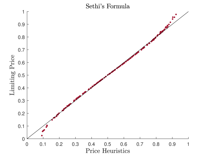
(a) Sethi’s heuristic price $\breve{p}$

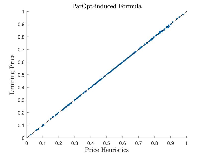
(b) Pareto Optimality-induced price $\hat{p}$

Figure 6. Comparison of the heuristic prices

A.6. Price Formula for Market with HARA Utility

In this section, we briefly discuss how to generalize the price formula derived from the CRRA-utility-based market to a more general utility family, namely, the utility with hyperbolic absolute risk aversion (HARA utility). We adopt similar notations in Section 5 and define the HARA utility-based MU functions as follows. Given wealth vectors $\mathbf{y}\in\mathbb{R}^{I}$ and $\mathbf{x}_{j}\in\mathbb{R}^{I}$, we assume the market maker’s MU function and the $j$-th trader’s MU function are

(71) $$U(\mathbf{y})\triangleq\frac{1-\gamma_{m}}{\gamma_{m}}\sum_{i=1}^{I}\theta_{i}\left(\frac{a_{m}y_{i}}{1-\gamma_{m}}+b_{m}\right)^{\gamma_{m}}~{}\textrm{and}~{}~{}V_{j}(\mathbf{x}_{j})\triangleq\frac{1-\gamma}{\gamma}\sum_{i=1}^{I}\pi_{i,j}\left(\frac{a_{j}x_{i,j}}{1-\gamma}+b_{j}\right)^{\gamma},$$

respectively, where $(\theta_{1},\ldots,\theta_{I})\in\Theta_{I}$ and $(\pi_{1,j},\ldots,\pi_{I,j})\in\Theta_{I}$ are the subjective beliefs, $\gamma_{m}$ and $\gamma$ are the risk aversion parameters of the market maker and the $j$-th trader, respectively; $a_{m}>0$, $b_{m}\geq 0$, $a_{j}>0$ and $b_{j}\geq 0$ for $j=1,2,\ldots,J$ are the parameters associated with the HARA utility functions. Clearly, CRRA utility is a special case of HARA utility. For examplem, if we set $b_{m}=0$ and $a_{m}=(1-\gamma_{m})^{\frac{\gamma_{m}-1}{\gamma_{m}}}$ in $U(\mathbf{y})$ it becomes the CRRA utility.

The above definitions of HARA utility-based MU functions satisfy the convergence conditions in Theorem 3.2. Thus, for a given trading sequence, the market state converges to a Pareto optimal point. We may solve problem $\mathcal{P}_{\textrm{po}}(\boldsymbol{\nu})$ with a set of weighting parameters $\boldsymbol{\nu}^{*}=(\nu_{1}^{*},\ldots,\nu_{J}^{*})$ for the Pareto optimal wealth allocation, i.e., we have the problem:

$$\mathcal{P}_{\textrm{po}}(\boldsymbol{\nu}^{*}):~{} ~{}\max_{\mathbf{y},\mathbf{x}_{1},\ldots,\mathbf{x}_{J}}~{}~{}~{}\frac{\gamma}{1-\gamma}\sum_{j=1}^{J}\left(\nu_{j}^{*}\cdot\sum_{i=1}^{I}\pi_{i,j}\left(\frac{a_{j}x_{i,j}}{1-\gamma}+b_{j}\right)^{\gamma}\right)$$

(72) Subject to: $$~{}\mathbf{y}+\sum_{j=1}^{J}\mathbf{x}_{j}={w}_{0}^{\textrm{all}}\cdot\mathbf{e},$$

(73) $$~{}\frac{\gamma_{m}}{1-\gamma_{m}}\sum_{i=1}^{I}\theta_{i}\left(\frac{a_{m}y_{i}}{1-\gamma_{m}}+b_{m}\right)^{\gamma_{m}}\geq U(W_{0})\triangleq\frac{\gamma_{m}}{1-\gamma_{m}}\left(\frac{a_{m}W_{0}}{1-\gamma_{m}}+b_{m}\right)^{\gamma_{m}}.$$

Similar to the CRRA utility, we have the optimality conditions:

(74) $$\nu_{j}^{*}\pi_{i,j}a_{j}\left(\frac{a_{j}x_{i,j}}{1-\gamma}+b_{j}\right)^{\gamma-1}=\xi,~{}~{}i=1,\ldots,I;j=1,\ldots,J,$$

(75) $$\eta\theta_{i}a_{m}\left(\frac{a_{m}y_{i}}{1-\gamma_{m}}+b_{m}\right)^{\gamma_{m}-1}=\xi,~{}~{}i=1,\ldots,I,$$

where $\boldsymbol{\xi}=(\xi_{1},\xi_{2},\ldots,\xi_{I})$ and $\eta\geq 0$ are the Lagrange multipliers for the two contratints. Using (75) in Eq. (73) gives

(76) $$\eta=\frac{\left(\frac{a_{m}W_{0}}{1-\gamma_{m}}+b_{m}\right)^{1-\gamma_{m}}}{\left(\sum\limits_{k=1}^{I}\theta_{k}\left(a_{m}\theta_{k}/\xi_{k}\right)^{\frac{\gamma_{m}}{1-\gamma_{m}}}\right)^{\frac{1-\gamma_{m}}{\gamma_{m}}}}.$$

Combining Eqs. (74), (75) and (76), we have the sytem of equations for $\boldsymbol{\xi}$:

$$(1-\gamma)\sum_{j=1}^{J}a_{j}^{-1}\left(\left(\frac{\nu_{j}^{*}\pi_{i,j}a_{j}}{\xi_{i}}\right)^{\frac{1}{1-\gamma}}-b_{j}\right)$$

(77) $$~{}~{}~{}~{}~{}~{}~{}~{}~{}~{}~{}~{}+\frac{1-\gamma_{m}}{a_{m}}\left(\left(\frac{\theta_{i}a_{m}}{\xi_{i}}\right)^{\frac{1}{1-\gamma_{m}}}\cdot\Big{(}\frac{a_{m}W_{0}}{1-\gamma_{m}}+b_{m}\Big{)}\cdot\mathcal{L}(\boldsymbol{\theta},\boldsymbol{\xi})-b_{m}\right)=w_{0}^{\textrm{all}},~{}~{}~{}i=1,\ldots,I,$$

where $\mathcal{L}(\boldsymbol{\theta},\boldsymbol{\xi})=\sum_{k=1}^{I}\theta_{k}(\theta_{k}/\xi_{k})^{\frac{\gamma_{m}}{1-\gamma_{m}}}$. Similar to the case of CRRA utility, the above equations admit a unique solution (see Appedix A.4), which we denote as $\xi^{*}=(\xi_{1}^{*},\ldots,\xi_{I}^{*})$. Then, the limiting price can be computed as

(78) $$p_{i}^{*}=\xi^{*}_{i}\Big{/}\sum\limits_{k=1}^{I}\xi_{k}^{*},~{}~{}i=1,\ldots,I.$$

In the market with a random trading sequence, we propose to use the following heuristic weights as an approximation,

(79) $$\hat{\nu}_{j}=\frac{1}{a_{j}}\Big{(}\frac{a_{j}w_{j,0}}{1-\gamma}+b_{j}\Big{)}^{1-\gamma},\quad\mbox{ for }j=1,2,\ldots,J.$$

Similar to the CRRA utility-based price formula, we may use the heuristic weight $\hat{\nu}_{j}$ to replace $\nu_{j}^{*}$ in Eq. (77). Then, solving these equations gives the solution $\hat{\boldsymbol{\xi}}=(\hat{\xi}_{1},\ldots,\hat{\xi}_{I})$. The associated approximate limiting price is $\hat{p}_{i}=\hat{\xi}_{i}/\sum_{k=1}^{I}\hat{\xi}_{k}$. In an unreported experiment, we find that the above approximation scheme accurately predicts the limiting price.

A.7. Trading Decision for Risk-Neutral Traders

We consider the case when the market maker adopts the exponential utility (given in (10)) and all the traders are risk neutral. Using the similar notations in Section 4.1, in $t$-th round of trading, the $j$-th trader interacts with the market. The market states are $\mathbf{y}_{t}=(y_{1,t},\ldots,y_{I,t})$ and $j$-the trader’s wealth is $\mathbf{x}_{j,t}=(x_{1,j,t},\ldots,x_{I,j,t})$. The $j$-th trader’s decision problem is as follows,

$$\max_{\mathbf{z}}~{}~{} ~{}\sum_{i=1}^{I}\pi_{i,j}(x_{i,j,t}+z_{i})$$

(80) Subject to $$~{}~{}~{}\sum_{i=1}^{I}\theta_{i}(1-e^{-\beta(y_{i}-z_{i})})\geq 1-e^{-\beta W_{0}}.$$

Checking the optimality condition, we get the optimal solution,

$$z_{i}^{*}=y_{i}-\frac{1}{\beta}\ln\left(\frac{\lambda\beta\theta_{i}}{\pi_{i,j}}\right),~{}~{}i=1,\ldots,I,$$

where $\lambda\geq 0$ is the Lagrange multiplier. It can be verified that $\lambda\not=0$. Thus the constraint (80) is binding for $z_{i}^{*}$, which gives the solution of $\lambda^{*}=\frac{1}{\beta}e^{\beta W_{0}}$. After the trading, the market state is updated to $y_{i,t+1}=y_{i,t}-z^{*}_{i}=\frac{1}{\beta}\ln\left(\frac{\lambda^{*}\beta\theta_{i}}{\pi_{i,j}}\right)$ for $i=1,\ldots,I$. The price is updated to

$$p_{i,t+1}=\frac{\theta_{i}e^{-\beta(y_{i}-z_{i}^{*})}}{\sum\limits_{k=1}^{I}\theta_{k}e^{-\beta(y_{k}-z_{k}^{*})}}=\pi_{i,j},$$

for $i=1,\ldots,I$. That is to say, after the $j$-th trader interacts with the market, the price is modified exactly according to the $j$-th trader’s belief.

Appendix B Properties of MU functions and Examples

B.1. Examples of MU Functions

One prominent feature of our framework is that it provides more freedom in designing multivariate utility function. The following example shows how various desirable objectives can be made explicit and combined with each other using our MU framework. We then provide some examples of MU functions which go beyond the conventional framework of Expected Utility or the Risk measure-based MU function. Let $I$ represent the number of securities, $(\theta_{1},\ldots,\theta_{I})\in\Theta$ denote the market maker’s belief, and $\mathbf{y}=(y_{1},\ldots,y_{I})$ the wealth vector.

• We may consider the following MU function,

  (81) $$U(\mathbf{y}) =-\frac{1}{\beta}\ln\left(\sum_{i=1}^{I}\theta_{i}e^{-\beta y_{i}}\right)+\eta\sum_{i=1}^{I}\theta_{i}\ln\big{(}y_{i}+B\big{)},$$

  where $\eta\geq 0$ is the parameter. The first term of $U(\mathbf{y})$ is the so called Entropic Risk Measure [Föllmer and Schied, 2011] and the second term represents the classical expected utility. It’s worth noting that the second term establishes an explicit lower bound of $-B$ for the market maker’s terminal wealth. In fact, if an explicit worst-case loss is desired, one can always add a penalty term $\frac{1}{\gamma}\sum_{i=1}^{I}\theta_{i}(y_{i}+B)^{\gamma}$ with $\gamma\leq 0$ to the original multivariate utility function $U(\mathbf{y})$.

• We can construct the following MU function,

  (82) $$U(\mathbf{y})=\min_{i=1,\ldots,I}~{}\{y_{i}\}+\frac{\eta}{\gamma}\big{(}\sum_{i=1}^{I}\theta_{i}y_{i}+B\big{)}^{\gamma},$$

  where $\eta\geq 0$ and $\gamma\leq 1$ are the paramter. In this MU function, the first term represents the worst-case terminal wealth for the market maker, and it is a concave function because it is the point-wise minimum of $\mathbf{y}$. The second term establishes a specific lower bound of $-B$ for the expectation, $\sum_{i=1}^{I}\theta_{i}y_{i}$. It’s important to note that as the parameter $\gamma$ approaches $1$, the second term approximates the expectation of the wealth (with a shift of $B$). Consequently, a market maker employing this MU function (82) may seek to strike a balance between minimizing worst-case losses and maximizing expectations.

• Using the MU framework, we can not only design the functional form of the MU function but also customize the domain of the MU function. Thus, it is possible to include some “hard constraint” on the market state in MU function. Specifically, consider the function $U(\mathbf{y})=\sum_{i=1}^{I}\theta_{i}u(y_{i})$ where $u(\cdot)$ is an conventional univariate utility function. We then define the domain of this MU function as

  $$\textbf{{dom}}(U)\triangleq\{\mathbf{y}:~{}\mathbf{y}\geq\mathbf{L}\}\cap\{\mathbf{y}:~{}\rho(\mathbf{y})\leq\rho_{0}\}\cap\{\mathbf{y}:~{}\sum_{i=1}^{I}\theta_{i}y_{i}\geq-B\},$$

  where $\rho_{0}(\cdot)$ can be viewed as some risk measure. As for the domain of the MU function, the first term bounds the worst-case loss, the second term bounds the risk, and the last term bounds the expectation of the wealth.

B.2. Equivalence Between Various Mechanisms

In this section, we explicitly assume the domain of $U$ is polyhedral: $\textbf{{dom}}(U)\triangleq\{\mathbf{y}:~{}\mathbf{a}_{k}^{\top}\mathbf{y}\geq b_{k},~{}\mathbf{a}_{k}>\mathbf{0},~{}k\in\mathcal{K}\}$ where $\mathcal{K}$ is some index set. The proof for the case $\textbf{{dom}}(U)=\mathbb{R}^{I}$ is similar.

A scoring rule $\mathbf{S}$ is a reward mechanism that prompts participants to report their subjective probability belief and pays them according to their predicting accuracy. Specifically, if someone reports $\mathbf{p}\in\Theta_{I}$, then he/she gets paid $\mathbf{S}(\mathbf{p})_{i}$ if outcome $i$ happens. A scoring rule is proper if truthfully reporting belief is a utility maximizing strategy for a myopic, risk-neutral participant. Additionally, it is strictly proper if truthful reporting is the only utility-maximizing strategy. [Hanson, 2003] invented a market implementation for scoring rules by transforming the belief reporting process into a sequential procedure.

Following a similar rationale with the Market Equivalence Theorem given by [Chen and Pennock, 2007], the following proposition shows how to retrieve a proper scoring rule from a multivariate utility function. We first introduce the following definition:

Definition B.1.

Consider a mapping $\mathbf{S}(\cdot)$ from a point to a set. If for any $\mathbf{p}_{n}\to\mathbf{p}^{*}$, $\mathbf{s}_{n}\in\mathbf{S}(\mathbf{p}_{n})$, it has $\lim_{n\to\infty}\mathbf{s}_{n}\in\mathbf{S}(\mathbf{p}^{*})$, then we say $\mathbf{S}(\cdot)$ is upper-hemicontinuous.

Proposition B.2.

If $U(\cdot):\mathbb{R}^{I}\rightarrow\mathbb{R}$ is a concave function and $U$-based pricing rule has bounded loss, for $\mathbf{p}\in\Theta_{I}$, we introduce $\mathbf{S}$ as,

(83) $$\mathbf{S}(\mathbf{p})\triangleq-{\arg\min} ~{}~{}\Big{\{}\mathbf{p}^{\top}\mathbf{y}~{}|~{}U(\mathbf{y})\geq U(W_{0}\cdot\mathbf{e}),~{}\mathbf{y}\in\textbf{{dom}}(U)\Big{\}},$$

where $\textbf{{dom}}(U)=\{\mathbf{y}:~{}\mathbf{a}_{k}^{\top}\mathbf{y}\geq b_{k},~{}\mathbf{a}_{k}>\mathbf{0},~{}k\in\mathcal{K}\}$, then $\mathbf{S}(\mathbf{p})$ is an upper-hemicontinuous correspondence on $\Theta_{I}$ and also a proper scoring rule. Furthermore, $\mathbf{S}(\cdot)$ is continuous within the interior of $\Theta_{I}$ when $U(\cdot)$ is strictly concave.

Proof of Proposition B.2. For convenience, we denote by $\mathcal{L}$$=$$\big{\{}\mathbf{y}~{}|~{}U(\mathbf{y})\geq U(W_{0}\cdot\mathbf{e}),~{}\mathbf{a}_{k}^{\top}\mathbf{y}\geq b_{k},~{}k\in\mathcal{K}\big{\}}$ the constraint set of (83). Since the market maker has bounded loss, then there exists a $\underline{\mathbf{y}}\in\mathbb{R}^{I}$ such that $\mathbf{y}\geq\underline{\mathbf{y}},~{}\forall\mathbf{y}\in\mathcal{L}$. This suggests that $\inf_{\mathbf{y}\in\mathcal{L}}\{\mathbf{e}_{i}^{\top}\mathbf{y}\}$ has a solution (possibly a set of extended reals). for all $i$. Then for any $\mathbf{p}\in\Theta_{I}$ we have $\inf_{\mathbf{y}\in\mathcal{L}}\{\mathbf{p}^{\top}\mathbf{y}\}\geq\sum_{i}p_{i}\inf_{\mathbf{y}\in\mathcal{L}}\{\mathbf{e}_{i}^{\top}\mathbf{y}\}$, which implies (83) has a solution for any $\mathbf{p}\in\Theta_{I}$. Specifically, for $\mathbf{p}\in\textrm{interior}(\Theta_{I})$ the intersection of recession cone of $\mathbf{p}^{\top}\mathbf{y}$ and $\mathcal{L}$ is $\{\mathbf{0}\}$, therefore the solution set is compact [Bertsekas et al., 2003], and the solution set is a unique element when $U$ is strictly concave, hence $\mathbf{S}:\textrm{interior}(\Theta_{I})\to\mathbb{R}^{I}$ is a function.

For the upper-hemicontinuity of $\mathbf{S}$, suppose there exists $\mathbf{p}_{n}\to\hat{\mathbf{p}}$, $\mathbf{s}_{n}\in\mathbf{S}(\mathbf{p}_{n})$ such that: $\lim_{n\to\infty}\mathbf{s}_{n}=\hat{\mathbf{s}}\not\in\mathbf{S}(\hat{\mathbf{p}})$. Here we consider extended reals, i.e., some elements of $\mathbf{s}_{n},\hat{\mathbf{s}}$ may be $+\infty$. Then we apply the Bolzano-Weistrass theorem on extended reals $\mathbf{s}_{n}$ to derive a convergence subsequence that converges to some $\hat{\mathbf{s}}$. By continuity of $U(\cdot)$, it has $U(-\hat{\mathbf{s}})\geq U(W_{0}\cdot\mathbf{e})$ and $-\mathbf{a}_{k}^{\top}\hat{\mathbf{s}}\geq b_{k}$ for all $k$. This means $\hat{\mathbf{s}}$ is a feasible solution for (83) at point $\hat{\mathbf{p}}$. Due to the optimality of $-\mathbf{S}(\hat{\mathbf{p}})$ at $\hat{\mathbf{p}}$, there exists an $\overline{\mathbf{s}}\in\mathbf{S}(\hat{\mathbf{p}})$ such that $-\hat{\mathbf{p}}^{\top}\overline{\mathbf{s}}<-\hat{\mathbf{p}}^{\top}\hat{\mathbf{s}}$. Again by continuity, monotonicity of $U(\cdot)$ and the fact that $\mathbf{a}_{k}>\mathbf{0},~{}k\in\mathcal{K}$, we can subtract a small $\epsilon\mathbf{e}$ from $\overline{\mathbf{s}}$ to get another $\tilde{\mathbf{s}}$ such that,

$$\begin{cases}-\hat{\mathbf{p}}^{\top}\tilde{\mathbf{s}}<-\hat{\mathbf{p}}^{\top}\hat{\mathbf{s}},\\ U(-\tilde{\mathbf{s}})>U(W_{0}\cdot\mathbf{e}),\\ -\mathbf{a}_{k}^{\top}\tilde{\mathbf{s}}>b_{k},~{}~{}k\in\mathcal{K}.\end{cases}$$

Since we have $\mathbf{p}_{n}\to\hat{\mathbf{p}}$, $\mathbf{s}_{n}\to\hat{\mathbf{s}}$, there exists an $N$ large enough such that the following system of inequalities hold,

$$\begin{cases}-\mathbf{p}_{N}^{\top}\tilde{\mathbf{s}}<-\mathbf{p}_{N}^{\top}\mathbf{s}_{N},\\ U(-\tilde{\mathbf{s}})>U(W_{0}\cdot\mathbf{e}),\\ -\mathbf{a}_{k}^{\top}\tilde{\mathbf{s}}>b_{k},~{}~{}k\in\mathcal{K}.\end{cases}$$

Such a fact means $\tilde{\mathbf{s}}$ is a feasible solution of (83) at $\mathbf{p}_{N}$, and its corresponding objective value is smaller than $\mathbf{s}_{N}$ which is a contradiction. Thus, when $\mathbf{p}_{n}\to\hat{\mathbf{p}}$, $\mathbf{s}_{n}\in\mathbf{S}(\mathbf{p}_{n})$ implies $\lim_{n\to\infty}\mathbf{s}_{n}=\hat{\mathbf{s}}\in\mathbf{S}(\hat{\mathbf{p}})$, i.e., $\mathbf{S}(\cdot)$ is upper-hemicontinuous. Furthermore, upper-hemicontinuity is equivalent with continuity when $\mathbf{S}(\cdot)$ is a function, therefore $\mathbf{S}$ is continuous on $\textrm{interior}(\Theta_{I})$ for a strictly concave MU function $U(\cdot)$.

As for properness, when a risk-neutral trader is facing a scoring rule $\mathbf{S}$, if we assume his/her true probability estimate is $\mathbf{p}$, then his/her decision problem can be expressed as,

(84) $$\max_{\mathbf{r}\in\Theta_{I}}{}{} ~{}~{}\mathbf{p}^{\top}\mathbf{s}$$

Subject to $$~{}~{}\mathbf{s}\in\mathbf{S}(\mathbf{r}),$$

$$~{}~{}\mathbf{S}(\mathbf{r})=-\underset{\mathbf{y}\in\mathcal{L}}{\arg\max}~{}-\mathbf{r}^{\top}\mathbf{y},$$

where $\mathcal{L}=\big{\{}\mathbf{y}:~{}U(\mathbf{y})\geq U(W_{0}\cdot\mathbf{e}),~{}~{}\mathbf{a}_{k}^{\top}\mathbf{y}\geq b_{k},~{}\forall k\big{\}}$. From the structure of such problem, it has

$$\mathbf{p}^{\top}\mathbf{s}_{1}\geq\mathbf{p}^{\top}\mathbf{s}_{2},\quad\forall\mathbf{r}\neq\mathbf{p},\mathbf{s}_{1}\in\mathbf{S}(\mathbf{p}),\mathbf{s}_{2}\in\mathbf{S}(\mathbf{r}),$$

which means truthfully reporting $\mathbf{p}$ is a utility-maximizing strategy. $\hfill\Box$

Remark 4.

From the above discussion one can also easily verify that the MU-induced scoring rule is strictly proper within the interior of $\Theta_{I}$ when the underlying utility is strictly concave.

The next proposition shows how to induce an MU with bounded loss from a proper scoring rule.

Proposition B.3.

Let $\mathbf{S}:\Theta_{I}\to R$ be a proper scoring rule and $\mathbf{S}$ is continuous on $\Theta_{I}$, let

$$\mathcal{L}\triangleq -\underset{\mathbf{p}\in\Theta_{I}}{\cap}\big{\{}\mathbf{s}:~{}\mathbf{p}^{\top}\mathbf{s}\leq\mathbf{p}^{\top}\mathbf{S}(\mathbf{p})\big{\}}$$

$$\mathcal{D}\triangleq ~{}~{}~{}\big{\{}\mathbf{S}(\mathbf{p}):~{}\mathbf{p}\in\Theta_{I}\big{\}}$$

then $\mathcal{L}$ is a closed and convex set and $-\mathcal{D}$ lie on the boundary of $\mathcal{L}$. Define

(85) $$U(\mathbf{y})\triangleq-\inf\{m:~{}\mathbf{y}+m\cdot\mathbf{e}\in\mathcal{L}\}=\underset{\mathbf{p}\in\Theta_{I}}{\inf}~{}\big{\{}\mathbf{p}^{\top}\big{(}\mathbf{S}(\mathbf{p})+\mathbf{y}\big{)}\big{\}}$$

then $U:\mathbb{R}^{I}\to\mathbb{R}$ is a weakly monotone multivariate utility function, while the $U$-based MU suffers bounded loss and satisfies

(86) $$-\mathbf{S}(\mathbf{r})\in\underset{\mathbf{y}}{\arg\min}~{}\big{\{}~{}\mathbf{r}^{\top}\mathbf{y}~{}|~{}U(\mathbf{y})\geq 0\big{\}}.$$

Proof of Proposition B.3. Clearly, $\big{\{}\mathbf{s}~{}|~{}\mathbf{p}^{\top}\mathbf{s}\leq\mathbf{p}^{\top}\mathbf{S}(\mathbf{p})\big{\}}$ defines a closed halfspace for all $\mathbf{p}\in\Theta_{I}$. Since closed halfspace is natively convex, $\mathcal{L}$ can be regarded as the intersection of closed convex sets. Thus, it is also closed and convex. Also, for $\mathbf{p}\in\Theta_{I}$, it is easy to see that $-\mathcal{D}$ lies on the boundary of $\mathcal{L}$.

Note that (85) can be expressed as,

$$U(\mathbf{y})\triangleq-\min_{m} ~{}~{}~{}\big{\{}~{}m~{}|~{}-\mathbf{p}^{\top}(\mathbf{y}+m\cdot\mathbf{e})\leq\mathbf{p}^{\top}\mathbf{S}(\mathbf{p}),\quad\forall\mathbf{p}\in\Theta_{I}\big{\}}.$$

The constraint set $-\mathbf{p}^{\top}(\mathbf{y}+m\cdot\mathbf{e})\leq\mathbf{p}^{\top}\mathbf{S}(\mathbf{p})$ for all $\mathbf{p}\in\Theta_{I}$ can be equivalently written as:

$$-\mathbf{p}^{\top}\mathbf{y}-m\leq\mathbf{p}^{\top}\mathbf{S}(\mathbf{p}),~{}~{}\forall\mathbf{p}\in\Theta_{I}\implies m\geq-\mathbf{p}^{\top}\big{(}\mathbf{S}(\mathbf{p})+\mathbf{y}\big{)},~{}~{}\forall\mathbf{p}\in\Theta_{I}.$$

Therefore MU function $U(\mathbf{y})$ is equivalent to

(87) $$U(\mathbf{y})=-\underset{\mathbf{p}\in\Theta_{I}}{\sup}~{}\big{\{}-\mathbf{p}^{\top}\big{(}\mathbf{S}(\mathbf{p})+\mathbf{y}\big{)}\big{\}}=\underset{\mathbf{p}\in\Theta_{I}}{\inf}~{}\big{\{}\mathbf{p}^{\top}\big{(}\mathbf{S}(\mathbf{p})+\mathbf{y}\big{)}\big{\}}.$$

At last, we check whether $U(\cdot)$ meets Assumption 1.

• Domain condition: Since $\mathbf{S}(\cdot)$ is continuous on $\Theta_{I}$, $U(\cdot)$ is actually defined as the negative of minimum value of a continuous function over a closed and compact set, then Weistrass Theorem says such minimum value is attainable and well-defined, therefore $U(\cdot)$ is well defined on whole $\mathbb{R}^{I}$.

• Continuity condition: Suppose $\mathbf{y}_{n}\to\overline{\mathbf{y}}$ but $U(\mathbf{y}_{n})$ does not approach $U(\overline{\mathbf{y}})$. Then, it must have one of the following cases:

  1. There exists a $\delta>0$ such that $\exists N>Z$, $U(\mathbf{y}_{N})>U(\overline{\mathbf{y}})+\delta,~{}~{}\forall Z>0$;

  2. There exists a $\delta>0$ such that $\exists N>Z,~{}U(\mathbf{y}_{N})+\delta<U(\overline{\mathbf{y}})$, $\forall Z>0$.

  Let $\mathbf{p}_{N}^{*}\in\underset{\mathbf{p}\in\Theta_{I}}{\arg\min}~{}\big{\{}\mathbf{p}^{\top}\big{(}\mathbf{S}(\mathbf{p})+\mathbf{y}_{N}\big{)}\big{\}}$ and $\overline{\mathbf{p}}^{*}\in\underset{\mathbf{p}\in\Theta_{I}}{\arg\min}~{}\big{\{}\mathbf{p}^{\top}\big{(}\mathbf{S}(\mathbf{p})+\overline{\mathbf{y}}\big{)}\big{\}}$. Then for case (1), by the continuity of $\mathbf{S}$ and $\mathbf{y}_{n}\to\overline{\mathbf{y}}$, we know there exists an $N$ sufficiently large such that

  $$U(\mathbf{y}_{N})={\mathbf{p}_{N}^{*}}^{\top}\big{(}\mathbf{S}(\mathbf{p}_{N}^{*})+\mathbf{y}_{N}\big{)}>{\overline{\mathbf{p}}^{*}}^{\top}\big{(}\mathbf{S}(\overline{\mathbf{p}}^{*})+\mathbf{y}_{N}\big{)},$$

  which is contradictory to the optimality of $\mathbf{p}_{N}^{*}$.

  As for case (2), there also exists an $N$ sufficiently large such that,

  $$U(\overline{\mathbf{y}})={\overline{\mathbf{p}}^{*}}^{\top}\big{(}\mathbf{S}(\overline{\mathbf{p}}^{*})+\overline{\mathbf{y}}\big{)}>{\mathbf{p}_{N}^{*}}^{\top}\big{(}\mathbf{S}(\mathbf{p}_{N}^{*})+\overline{\mathbf{y}}\big{)}$$

  which is contradictory to the optimality of $\overline{\mathbf{p}}^{*}$. Therefore, it must have $\mathbf{y}_{n}\to\overline{\mathbf{y}}\implies U(\mathbf{y}_{n})\to U(\overline{\mathbf{y}})$.

• Bounded loss condition: Since $\Theta_{I}$ is a closed and bounded set while $\mathbf{S}$ is continuous on $\Theta_{I}$, therefore, $\mathcal{D}=\big{\{}\mathbf{S}(\mathbf{p}):~{}\mathbf{p}\in\Theta_{I}\big{\}}$ is also a closed and bounded set. By the structure of $U$ we know $U(\mathbf{y})\geq 0\iff\mathbf{y}\in\mathcal{L}$. Since $\mathbf{e}_{i}\in\Theta_{I},~{}\forall i=1,\ldots,I$ then for any $\mathbf{y}$ satisfying $U(\mathbf{y})\geq 0$, it has:

  $$\mathbf{e}_{i}^{\top}\mathbf{y}\geq-\mathbf{e}_{i}^{\top}\mathbf{S}(\mathbf{e}_{i}),~{}~{}\forall i=1,\ldots,I,~{}\implies\inf_{U(\mathbf{y})\geq 0}y_{i}\geq-\mathbf{e}_{i}\mathbf{S}(\mathbf{e}_{i}),~{}~{}\forall i=1,\ldots,I.$$

  Since $\mathcal{D}$ is bounded, the left-hand side of the above inequality is also bounded, therefore the worst-case loss of the market maker is bounded.

• Concavity for $\mathbf{y}_{1},\mathbf{y}_{2}\in\mathbb{R}^{I}$: Note that the following inequality holds,

  $$U\big{(}\alpha\mathbf{y}_{1}+(1-\alpha)\mathbf{y}_{2}\big{)} =\underset{\mathbf{p}\in\Theta_{I}}{\inf}~{}\big{\{}\mathbf{p}^{\top}\big{(}\mathbf{S}(\mathbf{p})+\alpha\mathbf{y}_{1}+(1-\alpha)\mathbf{y}_{2}\big{)}\big{\}}$$

  $$\geq\alpha\underset{\mathbf{p}\in\Theta_{I}}{\inf}~{}\big{\{}\mathbf{p}^{\top}\big{(}\mathbf{S}(\mathbf{p})+\mathbf{y}_{1}\big{)}\big{\}}+(1-\alpha)\underset{\mathbf{p}\in\Theta_{I}}{\inf}~{}\big{\{}\mathbf{p}^{\top}\big{(}\mathbf{S}(\mathbf{p})+\mathbf{y}_{2}\big{)}\big{\}}$$

  $$=\alpha U(\mathbf{y}_{1})+(1-\alpha)U(\mathbf{y}_{2}).$$

• Weak monotonicity: The following inequalities holds true,

  $$U(\mathbf{y}+\bm{\delta}) =\underset{\mathbf{p}\in\Theta_{I}}{\inf}~{}\big{\{}\mathbf{p}^{\top}\big{(}\mathbf{S}(\mathbf{p})+\mathbf{y}+\bm{\delta}\big{)}\big{\}}\geq\underset{\mathbf{p}\in\Theta_{I}}{\inf}~{}\big{\{}\mathbf{p}^{\top}\big{(}\mathbf{S}(\mathbf{p})+\mathbf{y}\big{)}\big{\}}=U(\mathbf{y}),~{}~{}\forall\bm{\delta}\geq\mathbf{0},$$

  $$U(\mathbf{y}+\bm{\delta}) =\underset{\mathbf{p}\in\Theta_{I}}{\inf}~{}\big{\{}\mathbf{p}^{\top}\big{(}\mathbf{S}(\mathbf{p})+\mathbf{y}+\bm{\delta}\big{)}\big{\}}>\underset{\mathbf{p}\in\Theta_{I}}{\inf}~{}\big{\{}\mathbf{p}^{\top}\big{(}\mathbf{S}(\mathbf{p})+\mathbf{y}\big{)}\big{\}}=U(\mathbf{y}),$$

  $$~{}~{}~{}~{}~{}~{}~{}~{}~{}~{}~{}~{}\forall\bm{\delta}\mbox{ such that }\delta_{i}>0,~{}\forall i.$$

  Also for every $i$ and any $\mathbf{y}\in\mathbb{R}^{I}$ it has:

  $$U(\mathbf{y}-\beta\mathbf{e}_{i})=\underset{\mathbf{p}\in\Theta_{I}}{\inf}~{}\big{\{}\mathbf{p}^{\top}\big{(}\mathbf{S}(\mathbf{p})+\mathbf{y}-\beta\mathbf{e}_{i}\big{)}\big{\}}\leq\mathbf{e}_{i}^{\top}\mathbf{S}(\mathbf{e}_{i})+\mathbf{e}_{i}^{\top}\mathbf{y}-\beta.$$

  Since $\mathbf{e}_{i}^{\top}\mathbf{S}(\mathbf{e}_{i})+y_{i}$ is bounded for $\mathbf{y}\in\mathbb{R}^{I}$ and $\beta$ is arbitrary, for some $\beta>0$ it has $U(\mathbf{y}-\beta\mathbf{e}_{i})<U(\mathbf{y})$ for all $i$ and $\mathbf{y}\in\mathbb{R}^{I}$.

As for (86), first when $\mathbf{y}=-\mathbf{S}(\mathbf{r})$, by properness of $\mathbf{S}$ we have $\mathbf{p}^{\top}\mathbf{S}(\mathbf{p})-\mathbf{p}^{\top}\mathbf{S}(\mathbf{r})\geq 0,~{}~{}\forall\mathbf{p}\in\Theta_{I}$ therefore:

$$U\big{(}-\mathbf{S}(\mathbf{r})\big{)}=\inf_{\mathbf{p}\in\Theta_{I}}\big{\{}\mathbf{p}^{\top}\mathbf{S}(\mathbf{p})-\mathbf{p}^{\top}\mathbf{S}(\mathbf{r})\big{\}}\geq 0$$

which means $-\mathbf{S}(\mathbf{r})$ is a feasible solution of (86).

On the other hand, suppose there exists a $\tilde{\mathbf{y}}\in\mathbb{R}^{I}$ such that: $\mathbf{r}^{\top}\tilde{\mathbf{y}}<-\mathbf{r}^{\top}\mathbf{S}(\mathbf{r})$, which means

$$\mathbf{r}^{\top}\mathbf{S}(\mathbf{r})+\mathbf{r}^{\top}\tilde{\mathbf{y}}<0\implies U(\tilde{\mathbf{y}})=\inf_{\mathbf{p}\in\Theta_{I}}\big{\{}\mathbf{p}^{\top}\mathbf{S}(\mathbf{p})+\mathbf{p}^{\top}\tilde{\mathbf{y}}\big{\}}<0$$

that is to say any $\tilde{\mathbf{y}}$ with objective function value lower than $-\mathbf{r}^{\top}\mathbf{S}(\mathbf{r})$ is not a feasible solution of (86) therefore we must have $-\mathbf{S}(\mathbf{r})\in\underset{U(\mathbf{y})\geq 0}{\arg\min}~{}\mathbf{r}^{\top}\mathbf{y}$.

Cost function-based mechanism is a prediction market making method proposed by [Chen and Pennock, 2007]. It is now one of the most widely-used market making mechanism in prediction market literature due to its implementation simplicity. A cost function $C:\mathbb{R}^{I}\to\mathbb{R}$ should satisfy the following properties:

• $C(\cdot)$ is continuous and defined on whole $\mathbb{R}^{I}$;

• Convexity: $C(\alpha\mathbf{q}_{1}+(1-\alpha)\mathbf{q}_{2})\leq\alpha C(\mathbf{q}_{1})+(1-\alpha)C(\mathbf{q}_{2})$;

• Monotonicity: for any $\mathbf{q},\hat{\mathbf{q}}$, if $\mathbf{q}\geq\hat{\mathbf{q}}$, it has $C(\mathbf{q})\geq C(\hat{\mathbf{q}})$ and the inequality is held strictly if $\mathbf{q}>\hat{\mathbf{q}}$;

• Translation invariance: $C(\mathbf{q}+t\cdot\mathbf{e})=C(\mathbf{q})+t,~{}\forall t\in\mathbb{R}$.

Then given current outstanding securities $\mathbf{q}$, a new order $\Delta\mathbf{q}$ is charged with $C(\mathbf{q}+\Delta\mathbf{q})-C(\mathbf{q})$.

One can see that a $\rho(\mathbf{y})\triangleq C(-\mathbf{y})$ defines a risk measure, therefore $V(\mathbf{y})\triangleq-C(-\mathbf{y})$ is always a multivariate utility function. The following proposition formally establishes their equivalence.

Proposition B.4.

For any given $\mathbf{q}\in\mathbb{R}^{I}$ any multivariate-utility $U(\cdot)$, let

$$C_{U}(\mathbf{q})\triangleq\min ~{}~{}W$$

$$s.t. ~{}~{}U(W\cdot\mathbf{e}-\mathbf{q})\geq U(W_{0}\cdot\mathbf{e}),$$

$$~{}~{}W\cdot\mathbf{e}-\mathbf{q}\in\textbf{{dom}}(U),$$

then $C_{U}(\cdot)$ is a well-defined cost function, and $C_{U}(\mathbf{q}_{t}+\Delta\mathbf{q})-C_{U}(\mathbf{q}_{t})$ is exactly the price charge of $\Delta\mathbf{q}$ under $U$-based MU when outstanding securities are $\mathbf{q}_{t}$. Conversely, for any cost function $C(\cdot)$, let

(88) $$U_{C}(\mathbf{y})=-C(-\mathbf{y}),$$

then $U_{C}(\mathbf{y})$ is a qualified multivariate utility as per Assumption 1. Furthermore, denote by $W_{t}$ the amount of cash the cost function-based market maker collected by time $t$, then such a cost function-based market maker is equivalent to $U_{C}(W_{t}\cdot\mathbf{e}-\mathbf{q}_{t})=U_{C}(W_{0}\cdot\mathbf{e})$.

Proof of Proposition B.4. MU$\rightarrow$ Cost function: That $C_{U}$ is a function follows directly from uniqueness of solution of $\mathcal{P}_{\textrm{Cmin}}$; the translation invariance property is obvious. We now focus on the continuity and convexity of $C_{U}$:

• Continuity: Suppose there exists a sequence $\mathbf{q}_{n}\to\overline{\mathbf{q}}$ such that $\lim_{n\to\infty}C_{U}(\mathbf{q}_{n})=\hat{C}\neq C_{U}(\overline{\mathbf{q}})$ ($\hat{C}$ may be $+\infty$). If $\hat{C}>C_{U}(\overline{\mathbf{q}})$ , then $U(\hat{C}\cdot\mathbf{e}-\overline{\mathbf{q}})>U(C_{U}(\overline{\mathbf{q}})\cdot\mathbf{e}-\overline{\mathbf{q}})\geq U(W_{0}\cdot\mathbf{e})$, $\mathbf{a}_{k}^{\top}(\hat{C}\cdot\mathbf{e}-\overline{\mathbf{q}})>b_{k},~{}\forall k$. By continuity of $U$ we know there exists an $N$ sufficiently large such that: $U(C_{U}(\mathbf{q}_{N})\cdot\mathbf{e}-\mathbf{q}_{N})>U(W_{0}\cdot\mathbf{e})$, $\mathbf{a}_{k}^{\top}(C_{U}(\mathbf{q}_{N})\mathbf{e}-\mathbf{q}_{N})>b_{k},~{}\forall k$. Now we can achieve a smaller objective value by slightly reducing $C_{U}(\mathbf{q}_{N})$, which contradicts with the optimality of $C_{U}(\mathbf{q}_{N})$. Conversely, if $\hat{C}<C_{U}(\overline{\mathbf{q}})$, then by continuity of $U$ we have $U(\hat{C}\cdot\mathbf{e}-\overline{\mathbf{q}})\geq U(W_{0}\cdot\mathbf{e})$, $\mathbf{a}_{k}^{\top}(\hat{C}\cdot\mathbf{e}-\overline{\mathbf{q}})\geq b_{k},~{}\forall k$ , which again contradicts with the optimality of $C_{U}(\overline{\mathbf{q}})$. Therefore $\mathbf{q}_{n}\to\overline{\mathbf{q}}\implies C_{U}(\mathbf{q}_{n})\to C_{U}(\overline{\mathbf{q}})$, that is to say $C_{U}$ is continuous.

• Convexity: By the concavity of $U$ and the convexity of $\textbf{{dom}}(U)$ we know that for any $\mathbf{q}_{1},\mathbf{q}_{2}$:

  $$U\Big{(}\big{(}\alpha C_{U}(\mathbf{q}_{1})+(1-\alpha)C_{U}(\mathbf{q}_{2})\big{)}\cdot\mathbf{e}-\big{(}\alpha\mathbf{q}_{1}+(1-\alpha)\mathbf{q}_{2}\big{)}\Big{)}$$

  $$=U\Big{(}\alpha\big{(}C_{U}(\mathbf{q}_{1})\mathbf{e}-\mathbf{q}_{1}\big{)}+(1-\alpha)\big{(}C_{U}(\mathbf{q}_{2})\mathbf{e}-\mathbf{q}_{2}\big{)}\Big{)}$$

  $$\geq\alpha U\Big{(}C_{U}(\mathbf{q}_{1})\mathbf{e}-\mathbf{q}_{1}\Big{)}+(1-\alpha)U\Big{(}C_{U}(\mathbf{q}_{2})\mathbf{e}-\mathbf{q}_{2}\Big{)}$$

  $$\geq U(W_{0}\cdot\mathbf{e}).$$

  Similarly, it has

  $$\big{(}\alpha C_{U}(\mathbf{q}_{1})+(1-\alpha)C_{U}(\mathbf{q}_{2})\big{)}\cdot\mathbf{e}-\big{(}\alpha\mathbf{q}_{1}+(1-\alpha)\mathbf{q}_{2})\in\textbf{{dom}}(U),$$

  which means $\alpha C_{U}(\mathbf{q}_{1})+(1-\alpha)C_{U}(\mathbf{q}_{2})$ is a feasible solution of (88) at $\alpha\mathbf{q}_{1}+(1-\alpha)\mathbf{q}_{2}$, therefore by the optimality of $C_{U}(\cdot)$ we have:

  $$C_{U}(\alpha\mathbf{q}_{1}+(1-\alpha)\mathbf{q}_{2})\leq\alpha C_{U}(\mathbf{q}_{1})+(1-\alpha)C_{U}(\mathbf{q}_{2}).$$

The price equivalence between $C_{U}$ and (88) is obvious. $\square$

Cost function $\rightarrow$ MU: Clearly $U_{C}$ inherits concavity, continuity and monotonicity from $C$, therefore is a qualified risk preference function per Assumption 1. On the other hand, assume the cost function-based market maker has $W_{t}$ cash by time $t$, while the aggregate outstanding securities are $\mathbf{q}_{t}$ then the price charge for an incoming new order is $\Delta W_{t}=C(\mathbf{q}_{t}+\Delta\mathbf{q}_{t})-C(\mathbf{q}_{t})$. By translation invariance of $C$ it has

$$C(-(W_{t}+\Delta W_{t})\cdot\mathbf{e}+(\mathbf{q}_{t}+\Delta\mathbf{q}_{t}))= -W_{0}-\sum_{l=1}^{t-1}\big{(}C(\mathbf{q}_{l+1})-C(\mathbf{q}_{l})\big{)}$$

$$-\big{(}C(\mathbf{q}_{t}+\Delta\mathbf{q}_{t})+C(\mathbf{q}_{t})\big{)}-C(\mathbf{q}_{t}+\Delta\mathbf{q}_{t})$$

$$= -W_{0}=C(-W_{0}\cdot\mathbf{e}),$$

which further implies $U_{C}(W_{t}\cdot\mathbf{e}-\mathbf{q}_{t})=U_{C}(W_{0}\cdot\mathbf{e})$ for $t$. $\square$

B.3. Additional Properties of MU Function

• No-arbitrage for Surebet: Under Assumption 1, the market making mechanism induced by multivariate utility function $U(\cdot)$ is well defined and has the following properties.

  Proposition B.5.

  If the market maker adopts MU function $U(\cdot)$ to price any order $\Delta\mathbf{q}$ by solving problem $\mathcal{P}_{\textrm{cmin}}(\Delta\mathbf{q})$, it has following properties:

  (i):

  It can appropriately price any finite order $\Delta\mathbf{q}$ with finite price $\Delta w^{*}$ and the price $\Delta w^{*}$ is unique;

  (ii):

  The $k\in\mathbb{R}$ units of surebet order $\Delta\mathbf{q}=k\cdot\mathbf{e}$ is always charged with $k$ dollars.

  Proof.

  Proof. Given market state $(\mathbf{q},w)$ and incoming order $\{\Delta\mathbf{q}\}$, we denote the constraint set of $\mathcal{P}_{\textrm{cmin}}$ at this state by $\mathcal{C}(w,\mathbf{q},\Delta\mathbf{q})$. By the structure of the problem it is not hard to see that the only common direction of recession of set $\mathcal{C}(w,\mathbf{q},\Delta\mathbf{q})$ and objective function is $\mathbf{0}$, therefore $\mathcal{P}_{\textrm{cmin}}$ admits a solution for any $\{\mathbf{q},w\}$ and $\Delta\mathbf{q}$, and the solution is clearly unique. As for the price of surebet $\Delta q=k\mathbf{e}$, we consider two cases. In the first case, the market state $\{\mathbf{q},w\}$ resulted from previous trading satisfies $U(w\cdot\mathbf{e}-\mathbf{q})=U(W_{0}\cdot\mathbf{e})$. If we solve problem $\mathcal{P}_{\textrm{cmin}}$ for the surebet order $k\cdot\mathbf{e}$ in current round of trading, the constraint becomes $U((w+\Delta w)\cdot\mathbf{e}-(\mathbf{q}+k\cdot\mathbf{e}))\geq U(W_{0}\cdot\mathbf{e})$, which implies $\Delta w^{*}=k$. In the second case, if the previous trading gives $U(w\cdot\mathbf{e}-\mathbf{q})>U(W_{0}\cdot\mathbf{e})$, we may still have the solution $\Delta w^{*}=k$ for the order $k\cdot\mathbf{e}$. Otherwise, the previous trading may not achieve its optimal price. $\square$

• Bounded Worst-case Loss: Although a market maker is designed to provide liquidity, it is certainly not designed to be infinitely exploited. To avoid such catastrophe, one might wish to put a cap on the worst-case loss. Obviously MU function based market maker suffers bounded worst-case loss if and only if the utility level set $\mathcal{L}\triangleq\{\mathbf{y}\in\mathbb{R}^{I}~{}|~{}U(\mathbf{y})\geq U(W_{0}\cdot\mathbf{e})\}$ is lower bounded by some vector $\underline{\mathbf{y}}\in\mathbb{R}^{I}$, i.e., it has $\underline{\mathbf{y}}\leq\mathbf{y}$ for all $\mathbf{y}\in\mathcal{L}$. The utility level set $\mathcal{L}$ actually describes all the acceptable terminal wealth $\mathbf{y}$ of the market maker. Indeed, each element of $\underline{\mathbf{y}}=\big{(}\underline{y}_{1},\underline{y}_{2},\ldots,\underline{y}_{n}\big{)}$ can be characterized as follows,

  (89) $$\mathcal{P}_{i}~{} ~{}\min_{\mathbf{y}}\{y_{i}~{}|~{}\mathbf{y}=(y_{1},\cdots,y_{I}),~{}U(\mathbf{y})\geq U(W_{0}\cdot\mathbf{e})\}.$$

  Worst-case loss bound can be found by solving subproblems $\mathcal{P}_{i}$ for all $i=1,\cdots,I$. Obviously, the worst-case loss has a natural bound when the domain of utility $U$ itself is bounded from below, e.g., $U(\mathbf{y})=\sum_{i}\pi_{i}(y_{i}+B_{i})^{\gamma},~{}\gamma<1$. If such a domain bound design is not desired, then we need to find to other means to bound the loss. One viable way is to resort to transaction restrictions. Specifically, in real world traders are usually constrained to have non-negative wealth position when true state is revealed (It is known as the no-bankruptcy restriction). Under this case, bounded loss can be easily guaranteed. Besides the no-bankruptcy restriction, we provide the following results for the bounded worst-case loss.

  Proposition B.6.

  If multivariate utility function $U(\cdot)$ satisfies Assumption 1 and $\sup_{\mathbf{y}}U(\mathbf{y})=B<+\infty$ with

  (90) $$\lim\limits_{t\rightarrow\infty}U(t(\mathbf{e}-\mathbf{e}_{i}))<B,~{}~{}\textrm{for}~{}i=1,\cdots,I,$$

  then the MU-function based market maker has bounded loss.

  Proof.

  The multivariate utility function is bounded above means that, there exist some finite number $B$, such that $U(\mathbf{y})<B$ for any $\mathbf{y}\in\textbf{{dom}}(U)$. Under the condition given in this proposition, we assume the market maker has unbounded loss. Without loss of generality, we assume the first element of $\mathbf{y}$ may go to $-\infty$ and $y\in\mathcal{L}$. This assumption is equivalent to say there exists vector $\mathbf{y}(\tau)\triangleq(-\tau,g(\tau),g(\tau),\cdots,g(\tau))\in\mathbb{R}^{I}$ with $\mathbf{y}(\tau)\in\mathcal{L}$ when $\tau\rightarrow\infty$, where $\tau>0$ and $g(\tau)$ is any function satisfying $g(\tau)>\tau$. Clearly, it has $\mathbf{y}(\tau)=g(\tau)(\mathbf{e}-\mathbf{e}_{i})-\tau\mathbf{e}_{i}$. Since $U(\cdot)$ is a concave function, it has

  (91) $$\lim_{\tau\rightarrow\infty}U\big{(}g(\tau)(\mathbf{e}-\mathbf{e}_{i})-\tau\mathbf{e}_{i}\big{)}\leq\lim_{\tau\rightarrow\infty}\Big{(}U\big{(}g(\tau)(\mathbf{e}-\mathbf{e}_{i})\big{)}-\tau\nabla U(g(\tau)(\mathbf{e}-\mathbf{e}_{i}))^{\top}\mathbf{e}_{i}\Big{)}$$

  (92) $$\lim_{\tau\rightarrow\infty}U\big{(}g(\tau)(\mathbf{e}-\mathbf{e}_{i})+\sqrt{t}\mathbf{e}_{i}\big{)}\leq\lim_{\tau\rightarrow\infty}\Big{(}U(g(\tau)(\mathbf{e}-\mathbf{e}_{i}))+\sqrt{\tau}\nabla U\big{(}g(\tau)(\mathbf{e}-\mathbf{e}_{i})\big{)}^{\top}\mathbf{e}_{i}\Big{)}$$

  The left-hand side of inequality (92) tends to the infimum $B$. According to (90), it has $\lim_{\tau\rightarrow\infty}U(g(\tau)(\mathbf{e}-\mathbf{e}_{i}))<B$. Thus, there exists some $\delta>0$ satisfying $\delta=B-\lim\limits_{\tau\rightarrow\infty}U(g(\tau)(\mathbf{e}-\mathbf{e}_{i}))>0$. Also, inequality (92) becomes

  (93) $$\lim_{t\rightarrow\infty}\sqrt{t}\cdot\nabla U\big{(}g(t)(\mathbf{e}-\mathbf{e}_{i})\big{)}^{\top}\mathbf{e}_{i}\geq\delta$$

  Substituting the above inequality in (91) and noticing $\tau=\sqrt{\tau}\sqrt{\tau}$, it has

  $$\lim_{t\rightarrow\infty}U\big{(}g(\tau)(\mathbf{e}-\mathbf{e}_{i})-\tau\mathbf{e}_{i}\big{)} \leq\lim_{\tau\rightarrow\infty}\Big{(}F\big{(}g(\tau)(\mathbf{e}-\mathbf{e}_{i})\big{)}-\sqrt{\tau}\delta\Big{)}$$

  (94) $$<B-\lim_{\tau\rightarrow\infty}\sqrt{\tau}\delta=-\infty.$$

  That is to say, the utility of $U(\mathbf{y}(\tau))$ is infinitely low, thus can not be maintained above $U(W_{0}\cdot\mathbf{e})$. It contradicts our previous statement $\mathbf{y}(\tau)\in\mathcal{L}$, which also implies our assumption that $\mathcal{L}$ has no lower bound is not true. $\square$

• Acceptance of Limit Order: The MU-function based pricing rule can be easily modified to accept the limit order. We refer to $\mathbf{p}$ as the ‘instantaneous’ price since the actual price charge for any non-trivial order $\Delta\mathbf{q}$ is not $\mathbf{p}^{\top}\Delta\mathbf{q}$ but rather the amount $\Delta w^{*}$ calculated by solving problem $\mathcal{P}_{\textrm{cmin}}(\Delta\mathbf{q})$. This difference is due to the fact that the instantaneous price varies continuously along with the state variable $\mathbf{y}$. Such a phenomenon also persists in other mechanisms like the cost-function based mechanism. A limit order implementation could be a good rescue for this situation. The limit order could provide much more leeway for someone to express her valuation. [Agrawal et al., 2011] formally characterize a limit order by a triplet $(\mathbf{a},\Gamma,p^{\textrm{lim}})$, where $\mathbf{a}$ is a vector that describes the order by setting each component of $\mathbf{a}$ being either $1$ (if the specified state is desired) or $0$ (if it is not desired), $\Gamma\in\mathbb{R}$ denotes the maximum desired units of that bundle and $p^{\textrm{lim}}\in\mathbb{R}$ is the maximum averaged price the trader is willing to pay for the bundle. [Agrawal et al., 2011] shows that SCPM market maker decides the units to grant via solving a convex optimization problem. They also show that such implementation is a generalized Vickrey-Clarke-Groves(VCG) scheme(see, e.g., [Roughgarden, 2010]) and therefore admits myopic truthful reporting in the sense that traders will not lie about their true valuation of bid price $p^{\textrm{lim}}$. Similar to the SCPM, our MU function-based framework can be easily modified to incorporate limit order submission. Specifically, given market state $(\mathbf{q},w)$, a limit order of the form $(\mathbf{a},\Gamma,p^{\textrm{lim}})$, the price of this limit order can be computed by solving the following problem,

  (95) $$\mathcal{P}_{\textrm{Smax}}:~{}~{}\max_{0\leq\tau\leq\Gamma,\Delta w}{} ~{}p^{\textrm{lim}}\cdot\tau-\Delta w$$

  Subject to: $$~{}U((w+\Delta w)\cdot\mathbf{e}-(\mathbf{q}+\tau\mathbf{a}))\geq U(W_{0}\cdot\mathbf{e}),$$

  $$~{}(w+\Delta w)\cdot\mathbf{e}-(\mathbf{q}+\tau\mathbf{a})\in\textbf{{dom}}(U).$$

  After solving problem $\mathcal{P}_{Smax}$, the trader is granted $\tau^{*}$ shares and charged with $\Delta w^{*}$, where $(\tau^{*},\Delta w^{*})$ is the solution of problem $\mathcal{P}_{Smax}$. The objective function $\tau p^{\textrm{lim}}-\Delta w$ can be understood as follows. The term $\tau p^{\textrm{lim}}$ is the maximum price one is willing to pay for the order, and $\Delta w$ is the price actually charged for such an order. Maximizing $\tau p^{\textrm{lim}}-\Delta w$ is actually finding the highest possible cost reduction for the trader. Like SCPM, our limit order implementation is a generalized VCG scheme and admits truthful reporting of the bid price. The proof of this claim is similar to the one of Theorem 1 in [Agrawal et al., 2011]. Thus, we omit the details.

References

• Abbott [2001] Stephen Abbott. Understanding Analysis, volume 2. Springer, 2001.
• Abernethy et al. [2013] Jacob Abernethy, Yiling Chen, and Jennifer Wortman Vaughan. Efficient market making via convex optimization, and a connection to online learning. ACM Transactions on Economics and Computation, 1(2):1–39, 2013.
• Abernethy et al. [2014a] Jacob Abernethy, Sindhu Kutty, Sébastien Lahaie, and Rahul Sami. Information aggregation in exponential family markets. In Proceedings of the Fifteenth ACM Conference on Economics and Computation, pages 395–412, 2014a.
• Abernethy et al. [2014b] Jacob D. Abernethy, Rafael M. Frongillo, Xiaolong Li, and Jennifer Wortman Vaughan. A general volume-parameterized market making framework. In Proceedings of the Fifteenth ACM Conference on Economics and Computation, pages 413–430, 2014b.
• Agrawal et al. [2011] Shipra Agrawal, Erick Delage, Mark Peters, Zizhuo Wang, and Yinyu Ye. A unified framework for dynamic prediction market design. Operations Research, 59(3):550–568, 2011.
• Arrow et al. [2008] Kenneth J. Arrow, Robert Forsythe, Michael Gorham, Robert Hahn, Robin Hanson, John O. Ledyard, Saul Levmore, Robert Litan, Paul Milgrom, Forrest D. Nelson, George R. Neumann, Marco Ottaviani, Thomas C. Schelling, Robert J. Shiller, Vernon L. Smith, Erik Snowberg, Cass R. Sunstein, Paul C. Tetlock, Philip E. Tetlock, Hal R. Varian, Justin Wolfers, and Eric Zitzewitz. The promise of prediction markets. Science, 320(5878):877–878, 2008.
• Atanasov et al. [2022] P. Atanasov, J. Witkowski, B. Mellers, and P. Tetlock. Crowd prediction systems: Markets, polls, and elite forecasters. In Proceedings of the 23rd ACM Conference on Economics and Computation, pages 1013–1014, 2022.
• Atanasov et al. [2017] Pavel Atanasov, Phillip Rescober, Eric Stone, Samuel A Swift, Emile Servan-Schreiber, Philip Tetlock, Lyle Ungar, and Barbara Mellers. Distilling the wisdom of crowds: Prediction markets vs. prediction polls. Management Science, 63(3):691–706, 2017.
• Aumann [1976] Robert J Aumann. Agreeing to disagree. The Annals of Statistics, 4(6):1236–1239, 1976.
• Ban [2018] A. Ban. Strategy-proof incentives for predictions. In International Conference on Web and Internet Economics, pages 51–65. Springer, 2018.
• Barberis [2013] Nicholas C Barberis. Thirty years of prospect theory in economics: A review and assessment. Journal of Economic Perspectives, 27(1):173–196, 2013.
• Berg et al. [2008] Joyce E Berg, Forrest D Nelson, and Thomas A Rietz. Prediction market accuracy in the long run. International Journal of Forecasting, 24(2):285–300, 2008.
• Berg et al. [2009] Joyce E Berg, George R Neumann, and Thomas A Rietz. Searching for Google’s value: Using prediction markets to forecast market capitalization prior to an initial public offering. Management Science, 55(3):348–361, 2009.
• Bertsekas [2016] Dimitri Bertsekas. Nonlinear Programming. Athena, Scientific, 2016.
• Bertsekas et al. [2003] Dimitri P Bertsekas, Angelia Nedi, Asuman E Ozdaglar, et al. Convex Analysis and Optimization. Athena Scientific, 2003.
• Birge et al. [2021] J. R. Birge, Y. F. Feng, N. B. Keskin, and A. Schultz. Dynamic learning and market making in spread betting markets with informed bettors. Operations Research, 69(6):1446–1476, 2021.
• Bonnisseau and Nguenamadji [2013] Jean-Marc Bonnisseau and Orntangar Nguenamadji. Discrete Walrasian exchange process. Economic Theory, 52(3):1091–1100, 2013.
• Bordley [1982] R. F. Bordley. A multiplicative formula for aggregating probability assessments. Management Science, 28(10):1091–1213, 1982.
• Carvalho [2017] Arthur Carvalho. On a participation structure that ensures representative prices in prediction markets. Decision Support Systems, 104:13–25, 2017.
• Chakraborty and Das [2015] Mithun Chakraborty and Sanmay Das. Market scoring rules act as opinion pools for risk-averse agents. In Advances in Neural Information Processing Systems, pages 2359–2367, 2015.
• Chakravorti et al. [2023] T. Chakravorti, V. Singh, S. Rajtmajer, M. McLaughlin, R. Fraleigh, C. Griffin, A. Kwasnica, D. Pennock, and C. L. Giles. Artificial prediction markets present a novel opportunity for human-ai collaboration. In A. Ricci, W. Yeoh, N. Agmon, and B. An, editors, Proc. of the 22nd International Conference on Autonomous Agents and Multiagent Systems (AAMAS 2023), 2023.
• Chen et al. [2008] M Keith Chen, Jonathan E Ingersoll Jr, and Edward H Kaplan. Modeling a presidential prediction market. Management Science, 54(8):1381–1394, 2008.
• Chen and Pennock [2007] Yiling Chen and David M. Pennock. A utility framework for bounded-loss market makers. In Proceedings of the Twenty-Third Conference on Uncertainty in Artificial Intelligence, pages 49–56, 2007.
• Chen and Vaughan [2010] Yiling Chen and Jennifer Wortman Vaughan. A new understanding of prediction markets via no-regret learning. In Proceedings of the 11th ACM Conference on Electronic Commerce, pages 189–198. ACM, 2010.
• Chen et al. [2005] Yiling Chen, Chao-Hsien Chu, Tracy Mullen, and David M. Pennock. Information markets vs. opinion pools: An empirical comparison. In Proceedings of the 6th ACM Conference on Electronic Commerce, pages 58–67, 2005.
• Choo et al. [2022] Lawrence Choo, Todd R Kaplan, and Ro’i Zultan. Manipulation and (mis) trust in prediction markets. Management Science, 68(9):6716–6732, 2022.
• Cogwill and Zitzewitz [2015] Bo Cogwill and Eric Zitzewitz. Corporate prediction markets: Evidence from Google, Ford and Firm x. The Review of Economic Studies, 82(4):1309–1341, 2015.
• Cowgill et al. [2009] B. Cowgill, J. Wolfers, and Eric Zitzewitz. Auctions, Market mechanisms and Their Applications, chapter Using prediction markets to track information flows: Evidence from Google. Springer, 2009.
• den Boer and Keskin [2022] A. V. den Boer and N. B. Keskin. Dynamic pricing with demand learning and reference effects. Management Science, 68(10):7065–7791, 2022.
• Föllmer and Knispel [2015] Hans Föllmer and Thomas Knispel. Convex risk measures: Basic facts, law-invariance and beyond, asymptotics for large portfolios, chapter Chapter 30, pages 507–554. World Scientific Handbook in Financial Economics Series. World Scientific, 2015.
• Föllmer and Schied [2011] Hans Föllmer and Alexander Schied. Stochastic Finance: An Introduction in Discrete Time. Walter de Gruyter, 2011.
• Freeman and Pennock [2018] R. Freeman and D. M. Pennock. An axiomatic view of the parimutuel consensus wagering mechanism. In The 17th International Conference on Autonomous Agent and MultiAgent Systems, pages 1936–1938. ACM, 2018.
• Freeman et al. [2017] R. Freeman, D. M. Pennock, and J. Wortman Vaughan. The double clinching auction for wagering. In Proceeding of the 2017 ACM Conference on Economics and Computation, pages 43–60. ACM, 2017.
• Frongillo and Reid [2015] Rafael Frongillo and Mark D Reid. Convergence analysis of prediction markets via randomized subspace descent. In Advances in Neural Information Processing Systems 28, pages 3034–3042, 2015.
• Frongillo et al. [2015] Rafael Frongillo, Yiling Chen, and Ian Kash. Elicitation for aggregation. Proceedings of the AAAI Conference on Artificial Intelligence, 29(1):900–906, 2015.
• Gjerstad and Hall [2005] Steven Gjerstad and McClelland Hall. Risk aversion, beliefs, and prediction market equilibrium. Economic Science Laboratory, University of Arizona, 2005.
• Hanson [2003] Robin Hanson. Combinatorial information market design. Information Systems Frontiers, 5(1):107–119, 2003.
• Hanson [2007] Robin Hanson. Logarithmic markets scoring rules for modular combinatorial information aggregation. The Journal of Prediction Markets, 1(1):3–15, 2007.
• Hanson and Oprea [2009] Robin Hanson and Ryan Oprea. A manipulator can aid prediction market accuracy. Economica, 76(302):304–314, 2009.
• Healy et al. [2010] Paul J Healy, Sera Linardi, J Richard Lowery, and John O Ledyard. Prediction markets: Alternative mechanisms for complex environments with few traders. Management Science, 56(11):1977–1996, 2010.
• Hu and Storkey [2014] Jinli Hu and Amos Storkey. Multi-period trading prediction markets with connections to machine learning. In International Conference on Machine Learning, pages 1773–1781, 2014.
• Iyer et al. [2014] Krishnamurthy Iyer, Ramesh Johari, and Ciamac C Moallemi. Information aggregation and allocative efficiency in smooth markets. Management Science, 60(10):2509–2524, 2014.
• Jian and Sami [2010] Lian Jian and Rahul Sami. Aggregation and manipulation in prediction markets: Effects of trading mechanism and information distribution. In Proceedings of the 11th ACM Conference on Electronic Commerce, pages 207–208, 2010.
• Kahneman and Tversky [2013] Daniel Kahneman and Amos Tversky. Prospect theory: An analysis of decision under risk. In Handbook of the Fundamentals of Financial Decision Making: Part I, pages 99–127. World Scientific, 2013.
• Klenke [2013] Achim Klenke. Probability Theory: A Comprehensive Course. Springer Science & Business Media, 2013.
• Makarov and Schornick [2010] Dmitry Makarov and Astrid V Schornick. A note on wealth effect under CARA utility. Finance Research Letters, 7(3):170–177, 2010.
• Manski [2006] Charles F Manski. Interpreting the predictions of prediction markets. Economics Letters, 91(3):425–429, 2006.
• Mas-Colell et al. [1995] Andreu Mas-Colell, Michael Dennis Whinston, Jerry R Green, et al. Microeconomic Theory, volume 1. Oxford University Press New York, 1995.
• Morris [1974] P. A. Morris. Decision analysis expert use. Management Science, 20(9):1233–1241, 1974.
• Ostrovsky [2012] Michael Ostrovsky. Information aggregation in dynamic markets with strategic traders. Econometrica, 80(6):2595–2647, 2012.
• Othman and Sandholm [2010] Abraham Othman and Tuomas Sandholm. When do markets with simple agents fail? In Proceedings of the 9th International Conference on Autonomous Agents and Multiagent Systems: Volume 1, pages 865–872, 2010.
• Othman et al. [2013] Abraham Othman, David M. Pennock, Daniel M. Reeves, and Tuomas Sandholm. A practical liquidity-sensitive automated market maker. ACM Trans. Econ. Comput., 1(3):1–25, sep 2013.
• Pathak et al. [2015] Deepak Pathak, David Rothschild, and Miroslav Dudik. A comparison of forecasting methods: Fundamentals, polling, prediction markets, and experts. The Journal of Prediction Markets, 9(2):1–31, 2015.
• Pennock [1999] David M Pennock. Aggregating probabilistic beliefs: Market mechanisms and graphical representations. University of Michigan, 1999.
• Roughgarden [2010] Tim Roughgarden. Algorithmic game theory. Commun. ACM, 53(7):78–86, 2010.
• Sethi and Vaughan [2016] Rajiv Sethi and Jennifer Wortman Vaughan. Belief aggregation with automated market makers. Computational Economics, 48(1):155–178, 2016.
• Slamka et al. [2013] C. Slamka, B. Skiera, and M. Spann. Prediction market performance and market liquidity: A comparison of automated market makers. IEEE Transactions on Engineering Management, 60(1):169–185, 2013.
• Storkey et al. [2012] Amos Storkey, Jono Millin, and Krzysztof Geras. Isoelastic agents and wealth updates in machine learning markets. arXiv preprint arXiv:1206.6443, 2012.
• Tappe [2021] Stefan Tappe. Permutation invariant strong law of large numbers for exchangeable sequences. Journal of Probability and Statistics, 2021:3637837, 2021.
• Tarnaud [2019] Razvan Tarnaud. Convergence within binary market scoring rules. Economic Theory, 68(4):1017–1050, 2019.
• Tversky and Kahneman [1992] Amos Tversky and Daniel Kahneman. Advances in prospect theory: Cumulative representation of uncertainty. Journal of Risk and Uncertainty, 5(4):297–323, 1992.
• Wolfers and Zitzewitz [2004] Justin Wolfers and Eric Zitzewitz. Prediction markets. Journal of Economic Perspectives, 18(2):107–126, 2004.
• Wolfers and Zitzewitz [2006] Justin Wolfers and Eric Zitzewitz. Interpreting prediction market prices as probabilities. Technical report, National Bureau of Economic Research, 2006.
• Yu et al. [2022] D. Yu, J. J. Gao, and T. Y. Wang. Betting market equilibrium with heterogeneous beliefs: A prospect theory-based model. European Journal of Operational Research, 298:137–151, 2022.