Subspace-Based Detection and Localization in Distributed MIMO Radars

Abstract

In this paper, we consider a distributed multiple-input multiple-output (MIMO) radar which radiates waveforms with non-ideal cross- and auto-correlation functions and derive a novel subspace-based procedure to detect and localize multiple prospective targets. The proposed solution solves a sequence of composite binary hypothesis testing problems by resorting to the generalized information criterion (GIC); in particular, at each step, it aims to detect and localize one additional target, upon removing the interference caused by the previously-detected targets. An illustrative example is provided.

I Introduction

Distributed multiple-input multiple-output (MIMO) radars are equipped with widely-spaced transmitters and receivers that usually see different aspect angles of a prospective target [1, 2, 3, 4]. There are two main methodologies to perform detection and localization in these radar architectures. On the one hand, each receiver first elaborates its own data to identify candidate detections, while a fusion center makes a final decision on the target presence and performs its localization via triangulation [5, 6, 7]. On the other hand, the raw signals of all receivers are jointly elaborated to accomplish the desired task [8, 9, 10, 11]: this latter strategy will be considered next.

The works in [8, 9, 10] have discussed localization algorithms which rely upon the maximum likelihood estimation of the unknown parameters; however, these solutions do not consider the detection task and cannot handle an unknown target number. Joint detection and localization (JDL) is instead considered in [11]; however, this study assumes that the radiated waveforms have an all-zero cross-correlation and a thumb-tack auto-correlation function, so that a matched filter (MF) based receiver can be employed. However, such ideal correlation properties cannot be obtained in practice, and the resulting sidelobes can significantly degrade the performance [12, 13, 14, 15, 16, 17], if not properly accounted for in the design.

In this study, we consider the JDL of multiple targets in a distributed MIMO radar with an imperfect waveform separation. Interestingly, a somehow similar problem has been recently considered in the context of mmWave dual-function radar-communication systems [18, 19, 20, 21] and of passive radars [22, 23]. Inspired by these related studies, we make the following contributions. We show that the superposition of the echoes produced by each target in response to waveforms emitted by the radar transmitters can be regarded as a subspace signal, whose structure is specified by the target location. Following the design methodology in [21], we derive a novel iterative subspace-based detector that extracts one target at the time from the data and is robust to the sidelobe masking caused by the stronger targets on weaker ones. The proposed procedure generalizes the one discussed in [21] to the case where multiple widely-spaced transmitters/receivers are present and the targets belong to linear subspaces which may be not independent. Finally, we assess the performance of the proposed detector, also in comparison with the solution in [11] and the single-target benchmark.

The remainder of this work is organized as follows. Sec. II contains the signal model. Sec. III presents the proposed algorithm. Sec. IV provides the numerical analysis. Finally, the conclusions are given in Sec. V.

II Signal Model

Consider a distributed MIMO radar with $N$ transmitters located at $\{\bm{x}^{\rm tx}_{n}\}_{n=1}^{N}$ and $P$ receivers located at $\{\bm{x}^{\rm rx}_{p}\}_{p=1}^{P}$, with $\bm{x}^{\rm tx}_{n},\bm{x}^{\rm rx}_{p}\in\mathbb{R}^{2}$; the $n$-th transmitter emits the signal $\tilde{s}_{n}(t)$ which has a two-sided bandwidth $W$ and supports in $[0,T]$, with $WT\gg N$. Let $f_{\max}\geq 0$ be the maximum magnitude of the Doppler shift in any target echo, we assume $f_{\max}T\ll 1$, so that such Doppler shift can be neglected. If $K\in\{0,1,\ldots,K_{\max}\}$ point-like targets are present, the baseband signal observed by the $p$-th receiver is [8]

$$\tilde{r}_{p}(t)=\sum_{k=1}^{K}\sum_{n=1}^{N}a_{p,n,k}\tilde{s}_{n}\big{(}t-\tau_{p,n}(\bm{x}_{k})\big{)}+\tilde{w}_{p}(t)$$ (1)

for $p=1,\ldots,P$. Here, $\tilde{w}_{p}(t)$ is the additive noise, modeled as a complex circularly-symmetric Gaussian process independent across the receivers. Also, the first term on the right hand side is present only if $K\geq 1$; in this case, $\bm{x}_{k}\in\mathbb{R}^{2}$ is the location of the $k$-th target, while $a_{p,n,k}\in\mathbb{C}$ and $\tau_{p,n}(\bm{x}_{k})=\|\bm{x}^{\rm rx}_{p}-\bm{x}_{k}\|/c+\|\bm{x}^{\rm tx}_{n}-\bm{x}_{k}\|/c$ are the amplitude and the delay of its echo with respect to the receiver/transmitter pair $(p,n)$, respectively, and $c$ is the speed of light. The number of targets and their amplitudes and locations are unknown.

To remove the out-of-bandwidth noise, $\tilde{r}_{p}(t)$ is sent to a low-pass filter, whose impulse response $\phi(t)$ has support in $[0,T_{\phi}]$. Upon defining $r_{p}(t)=\tilde{r}_{p}(t)\star\phi(t)$, $s_{n}(t)=\tilde{s}_{n}(t)\star\phi(t)$, and $w_{p}(t)=\tilde{w}_{p}(t)\star\phi(t)$, we have

$$r_{p}(t)=\sum_{k=1}^{K}\sum_{n=1}^{N}a_{p,n,k}s_{n}\big{(}t-\tau_{p,n}(\bm{x}_{k})\big{)}+w_{p}(t).$$ (2)

We make here the standard assumption that two copies of $s_{n}(t)$ with delay $\delta_{1}$ and $\delta_{2}$ are resolvable if $|\delta_{1}-\delta_{2}|>1/W$, and, following [11], we say that $K\geq 2$ targets located at $\{\bm{x}_{k}\}_{k=1}^{K}$ are separable if, for any target pair $(k,q)$, with $k\neq q$, there exists at least one receiver/transmitter pair $(p,n)$ such that $s_{n}\big{(}t-\tau_{p,n}(\bm{x}_{k})\big{)}$ and $s_{n}\big{(}t-\tau_{p,n}(\bm{x}_{q})\big{)}$ are resolvable,

Finally, $r_{p}(t)$ is sampled at rate $1/T_{s}$ in the interval $\mathcal{I}=[\tau_{\min},T+T_{\phi}+\tau_{\max})$, where $\tau_{\min}$ and $\tau_{\max}$ are the minimum and maximum delays of a prospective echo, respectively; the $M=\left\lceil(T+T_{\phi}+\tau_{\max}-\tau_{\min})/T_{s}\right\rceil$ data samples are organized into the following $M$-dimensional vector

$$\bm{r}_{p}=\sum_{k=1}^{K}\bm{S}_{p}(\bm{x}_{k})\bm{a}_{p,k}+\bm{w}_{p}$$ (3)

where $\bm{S}_{p}(\bm{x}_{k})=\left[\bm{s}_{p,1}(\bm{x}_{k})\,\cdots\,\bm{s}_{p,N}(\bm{x}_{k})\right]\in\mathbb{C}^{M\times N}$, $\bm{s}_{p,n}(\bm{x}_{k})$ contains the samples $\big{\{}s_{n}\big{(}(m-1)T_{s}+\tau_{\min}-\tau_{p,n}(\bm{x}_{k})\big{)}\big{\}}_{m=1}^{M}$ and represents the signature of the echo generated by the $k$-th target towards the $p$-th receiver when illuminated by the $n$-th transmitter, $\bm{a}_{p,k}=(a_{p,1,k},\ldots,a_{p,N,k})^{\top}\in\mathbb{C}^{N}$, and $\bm{w}_{p}\in\mathbb{C}^{M}$ is a complex circularly-symmetric Gaussian vector with full-rank covariance matrix $\bm{C}_{p}$.

III Proposed Subspace-Based Detector

We aim to jointly detect and localize multiple targets, given only the location of the transmitters and receivers, the emitted waveforms, and the measurement vectors $\bm{r}_{1},\ldots,\bm{r}_{P}$. To proceed, notice that $\bm{r}_{p}$ is the noisy superposition of an unknown number of subspace signals originated from as many targets; the $k$-th subspace signal belongs to the column span of the mode matrix $\bm{S}_{p}(\bm{x}_{k})$, which only depends upon the target location $\bm{x}_{k}$. Leveraging the design methodology in [21], we propose to solve a sequence of composite binary hypothesis testing problems: in each problem, we aim to detect a subspace signal generated by a prospective target with an unknown location in the presence of the subspace interference caused by the previously-detected targets plus independent noise.

As customary, we start by assuming that the targets are located on a finite grid, say $\mathcal{G}$, whose points are uniformly-spaced in the inspected region and have an inter-element spacing $\Delta_{g}\leq c/W$; also, we restrict the search to targets which are at least separable. Let $\hat{\bm{x}}^{(k)}$ be the estimated location of the target detected in the $k$-th iteration; also, let $\mathcal{G}^{(k)}$ be the search set in the $k$-th iteration, with $\mathcal{G}^{(1)}=\mathcal{G}$ and

$$\mathcal{G}^{(k)}=\Big{\{}\bm{g}\in\mathcal{G}^{(k-1)}:\\ \min_{i\in\{1,\ldots,k-1\}}\max_{\begin{subarray}{c}p\in\{1,\ldots,P\}\\ n\in\{1,\ldots,N\}\end{subarray}}\;\big{|}\tau_{p,n}(\bm{g})-\tau_{p,n}(\hat{\bm{x}}^{(i)})\big{|}>\frac{1}{W}\Big{\}}$$ (4)

for $k\geq 2$. Then, the $k$-th testing problem to be solved is

$$\begin{cases}\mathcal{H}^{(k)}_{0}:&\displaystyle\bm{r}_{p}=\sum_{i=1}^{k-1}\bm{S}_{p}(\hat{\bm{x}}^{(i)})\bm{a}_{p}^{(i)}+\bm{w}_{p},\;\forall\;p\\[5.0pt] \mathcal{H}^{(k)}_{1}:&\displaystyle\bm{r}_{p}=\bm{S}_{p}(\bm{x}^{(k)})\bm{a}_{p}^{(k)}\\ &\displaystyle\hskip 22.76228pt+\sum_{i=1}^{k-1}\bm{S}_{p}(\hat{\bm{x}}^{(i)})\bm{a}_{p}^{(i)}+\bm{w}_{p},\;\forall\;p\end{cases}$$ (5)

for $k=1,2,\ldots,K_{\max}$. At the $p$-th receiver, $\bm{S}_{p}(\bm{x}^{(k)})\in\mathbb{C}^{M\times N}$ is the mode matrix of a prospective target located in $\bm{x}^{(k)}\in\mathcal{G}^{(k)}$, while $\bm{a}_{p}^{(k)}=\text{cat}\big{\{}a_{p,1}^{(k)},\ldots,a_{p,N}^{(k)}\big{\}}\in\mathbb{C}^{N}$ is the corresponding unknown gain vector; also, for $k\geq 2$, $\bm{S}_{p}(\hat{\bm{x}}^{(i)})\in\mathbb{C}^{M\times N}$ is the mode matrix of the interference caused by the target detected in the $i$-th iteration, while $\bm{a}_{p}^{(i)}\in\mathbb{C}^{N}$ is the corresponding unknown gain vector, for $i=1,\ldots,k-1$. The negative log-likelihood functions under $\mathcal{H}_{0}^{(k)}$ and $\mathcal{H}_{1}^{(k)}$ at the $p$-th receiver are

$$-\ln{{f}_{p,0}^{(k)}}\big{(}{\bm{r}_{p}};\bm{\alpha}_{p,0}^{(k)}\big{)}=\ln\Big{(}\pi^{M}\det\bm{C}_{p}\Big{)}\\ +\Big{\|}\bm{C}_{p}^{-1/2}\Big{(}{\bm{r}_{p}}-\bm{\Sigma}_{p,0}^{(k)}\bm{\alpha}_{p,0}^{(k)}\Big{)}\Big{\|}^{2}$$ (6)

and

$$-\ln{{f}_{p,1}^{(k)}}\big{(}{\bm{r}_{p}};\bm{x}^{(k)},\bm{\alpha}_{p,1}^{(k)}\big{)}=\ln\Big{(}\pi^{M}\det\bm{C}_{p}\Big{)}\\ +\Big{\|}\bm{C}_{p}^{-1/2}\Big{(}{\bm{r}_{p}}-\bm{\Sigma}_{p,1}^{(k)}(\bm{x}^{(k)})\bm{\alpha}_{p,1}^{(k)}\Big{)}\Big{\|}^{2}$$ (7)

respectively, where

$$\bm{\Sigma}_{p,0}^{(k)} =\begin{bmatrix}\bm{S}_{p}(\hat{\bm{x}}^{(1)})&\cdots&\bm{S}_{p}(\hat{\bm{x}}^{(k-1)})\end{bmatrix}\in\mathbb{C}^{M\times(k-1)N}$$ (8a)

$$\bm{\alpha}_{p,0}^{(k)} =\text{cat}\big{\{}\bm{a}_{p}^{(1)},\ldots,\bm{a}_{p}^{(k-1)}\big{\}}\in\mathbb{C}^{(k-1)N}$$ (8b)

are the augmented mode matrix and gain vector of the interference under $\mathcal{H}_{0}^{(k)}$, while

$$\bm{\Sigma}_{p,1}^{(k)}(\bm{x}^{(k)}) =\begin{bmatrix}\bm{\Sigma}_{p,0}^{(k)}&&&\bm{S}_{p}(\bm{x}^{(k)})\end{bmatrix}\in\mathbb{C}^{M\times kN}$$ (9a)

$$\bm{\alpha}_{p,1}^{(k)} =\text{cat}\big{\{}\bm{\alpha}_{p,0}^{(k)},\bm{a}_{p}^{(k)}\big{\}}\in\mathbb{C}^{kN}$$ (9b)

are the augmented mode matrix and gain vector accounting for the target and the interference under $\mathcal{H}_{1}^{(k)}$. Accordingly, it can be verified that the decision rule based upon the generalized information criterion (GIC) is

$$\max_{\bm{x}^{(k)}\in\mathcal{G}^{(k)}}\mathcal{J}^{(k)}(\bm{x}^{(k)})\mathrel{\underset{\mathcal{H}^{(k)}_{0}}{\overset{\mathcal{H}^{(k)}_{1}}{\gtrless}}}0$$ (10)

where

$$\mathcal{J}^{(k)}(\bm{x}^{(k)}) =\sum\limits_{p=1}^{P}\bigg{(}\Big{\|}{\bm{\Pi}}_{p}^{(k)}(\bm{x}^{(k)})\bm{C}_{p}^{-1/2}{\bm{r}_{p}}\Big{\|}^{2}$$

$$\quad-\eta\,\text{rank}\Big{\{}{\bm{\Pi}}_{p}^{(k)}(\bm{x}^{(k)})\Big{\}}\bigg{)}$$ (11)

$${\bm{\Pi}}_{p}^{(k)}(\bm{x}^{(k)}) =\Big{(}\bm{I}_{M}-{\bm{\Xi}}_{p}^{(k)}\Big{)}\bm{C}_{p}^{-1/2}\bm{S}_{p}(\bm{x}^{(k)})$$

$$\quad\times\Big{(}\Big{(}\bm{I}_{M}-{\bm{\Xi}}_{p}^{(k)}\Big{)}\bm{C}_{p}^{-1/2}\bm{S}_{p}(\bm{x}^{(k)})\Big{)}^{+}.$$ (12)

The following remarks are now in order. The matrix ${\bm{\Xi}}_{p}^{(k)}$ is the orthogonal projector on the interference subspace spanned by the columns of $\bm{C}_{p}^{-1/2}\bm{\Sigma}_{p,0}^{(k)}$, with the understanding that ${\bm{\Xi}}_{p}^{(k)}$ is the all-zero $M\times M$ matrix for $k=1$. The matrix ${\bm{\Pi}}_{p}^{(k)}(\bm{x}^{(k)})$ is the orthogonal projector on the part of the column space of $\bm{C}_{p}^{-1/2}\bm{S}_{p}(\bm{x}^{(k)})$ not contained in the interference subspace. In (11), $\big{\|}{\bm{\Pi}}_{p}^{(k)}(\bm{x}^{(k)})\bm{C}_{p}^{-1/2}{\bm{r}_{p}}\big{\|}^{2}$ is the energy of the whitened measurement $\bm{C}_{p}^{-1/2}{\bm{r}_{p}}$ contained in the subspace spanned by the column of ${\bm{\Pi}}_{p}^{(k)}(\bm{x}^{(k)})$, while $\text{rank}\big{\{}{\bm{\Pi}}_{p}^{(k)}(\bm{x}^{(k)})\big{\}}$ is the model order under $\mathcal{H}^{(1)}_{k}$ and $\eta$ is a penalty factor. Finally, the decision rule in (10) compares the maximum value of the scoring metric in (11) over all points in $\mathcal{G}^{(k)}$ with a threshold. When $\mathcal{H}_{1}^{(k)}$ is accepted, then the estimated location $\hat{\bm{x}}^{(k)}$ of the $k$-th detected target is the argument of the maximum.

The proposed decision logic sequentially solves the testing problems in (10) until no additional target is found or $\mathcal{G}^{(k+1)}=\emptyset$ or $k=K_{\max}$. If the procedure terminates at iteration $\hat{K}$, the number of detected targets is $\hat{K}-1$ if the detection threshold has not been crossed in the last test and $\hat{K}$ otherwise. We choose the penalty factor $\eta$ to obtain a desired probability of false alarm, namely, $\text{P}_{\text{fa}}=\text{Pr}\big{(}\max_{\hat{\bm{x}}^{(1)}\in\mathcal{G}^{(1)}}\mathcal{J}^{(1)}(\hat{\bm{x}}^{(1)})>0\text{ under }\mathcal{H}_{0}^{(1)}\big{)}$. The overall procedure is referred to as the matched subspace detector with iterative estimation of the interference subspace (MSD-IS).

III-A Mitigation of Small-Scale Localization Errors

Small-scale localization errors due to the off-grid target placement may be detrimental in the implementation of the MSD-IS, as the estimated interference subspace at iteration $k\geq 2$ may not fully contain the echoes of the $k-1$ previously-detected targets. We describe next a practical fix.

Let $\tilde{\mathcal{G}}\supset\mathcal{G}$ be a finer grid of points uniformly-spaced in the inspected region, with inter-element spacing $\tilde{\Delta}_{g}\ll\Delta_{g}$, and let $\mathcal{B}^{(i)}=\big{\{}\bm{g}\in\tilde{\mathcal{G}}:\;\big{\|}\bm{g}-\hat{\bm{x}}^{(i)}\big{\|}\leq c/W\big{\}}$ be the set containing the points in $\tilde{\mathcal{G}}$ close to $\hat{\bm{x}}^{(i)}$; finally, let $\bm{E}_{p,n}^{(i)}$ be the $M\times|\mathcal{B}^{(i)}|$ matrix whose columns are the signatures $\{\bm{s}_{p,n}(\bm{g})\}_{\bm{g}\in\mathcal{B}^{(i)}}$. After interference rejection, at the $p$-th receiver, we assume that the $n$-th echo of the target detected in the $i$-th iteration belongs to the augmented subspace spanned by the columns of $\big{(}\bm{I}_{M}-{\bm{\Xi}}_{p}^{(i)}\big{)}\bm{C}_{p}^{-1/2}\bm{E}_{p,n}^{(i)}$. Since this matrix contains signatures corresponding to non-resolvable delays, it may be ill-conditioned and some care is required to avoid an unnecessary subspace enlargement. Let $\lambda_{p,n,1}^{(i)},\ldots,\lambda_{p,n,B^{(i)}}^{(i)}$ be its squared singular values of arranged in a decreasing ordering and let $\bm{u}_{p,n,1}^{(i)},\ldots,\bm{u}_{p,n,B^{(i)}}^{(i)}$ be the corresponding left singular vectors; then, we only retain the left singular vectors corresponding to the ${U}_{p,n}^{(i)}$ largest singular values, where ${U}_{p,n}^{(i)}\geq 1$ is the smaller index such that

$$\frac{\big{|}\hat{a}_{p,n}^{(k)}\big{|}^{2}}{|\mathcal{B}^{(i)}|}\sum_{m=U_{p,n}^{(i)}+1}^{|\mathcal{B}^{(i)}|}\lambda_{p,n,m}^{(i)}<\epsilon$$ (13)

and $\epsilon$ is a parameter ruling the significance of the singular values with respect to the noise floor. At this point, the matrix ${\bm{\Xi}}_{p}^{(k)}$ used in (12) is replaced by the orthogonal projector on the augmented interference subspace spanned by

$$\Big{\{}\Big{\{}\bm{u}_{p,n,1}^{(i)},\ldots,\bm{u}_{p,n,U_{p,n}^{(i)}}^{(i)}\Big{\}}_{n=1}^{N}\Big{\}}_{i=1}^{k-1}.$$ (14)

IV Numerical Results

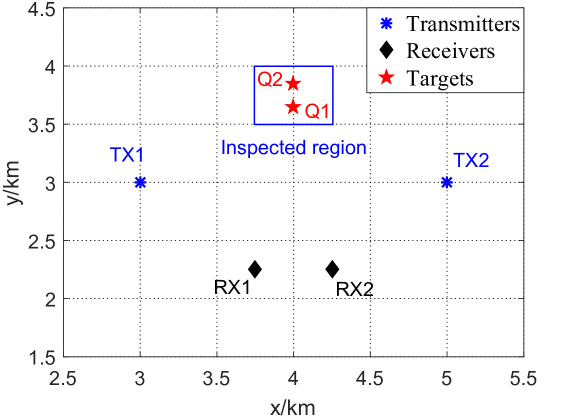
Figure 1: The positions of the transmitters, receivers and targets.

In the following example, we consider the $2\times 2$ MIMO radar in Fig. 1 with two targets (namely, $\text{Q}_{1}$ and $\text{Q}_{2}$) located at $\bm{x}_{1}=(4000,3650)\leavevmode\nobreak\ \text{m}$ and $\bm{x}_{2}=(4000,3850)\leavevmode\nobreak\ \text{m}$. The signal-to-noise ratio (SNR) of the $k$-th target is defined as

$$\text{SNR}_{k}=\frac{1}{NP}\sum_{n=1}^{N}\sum_{p=1}^{P}|a_{p,n,k}|^{2}\|\bm{C}_{w,p}^{-1/2}\bm{s}_{p,n}(\bm{x}_{k})\|^{2}.$$ (15)

Also, we consider the following time-coded radar waveforms

$$\tilde{s}_{n}(t)=\sum_{\ell=1}^{64}b_{n,\ell}\psi\big{(}t-(\ell-1)T/64\big{)},\quad n=1,\ldots,N$$ (16)

where $\psi(t)$ is a rectangular pulse with support in $[0,T/64]$ and $b_{n,1},\ldots,b_{n,64}$ is a random four-phase code sequences. Finally, $K_{\max}=5$, $W=10\leavevmode\nobreak\ \text{MHz}$, $\phi(t)=\sqrt{64/T}\psi(t)$, $T=6.4\leavevmode\nobreak\ \textmu\text{s}$, $T_{s}=0.05\leavevmode\nobreak\ \textmu\text{s}$, $\text{P}_{\text{fa}}=10^{-3}$, $\Delta_{g}=10$ m, $\tilde{\Delta}_{g}=0.05$ m, and $\text{SNR}_{2}/\text{SNR}_{1}=4$. We assume that target $\text{Q}_{1}$ is the one of interest, and the system performance is assessed in terms of its probability of detection ($\text{P}_{\text{d}}$) and the root mean square error (RMSE) in the estimation of its position. For comparison, we also include the performance obtained with the JDL algorithm with successive interference cancellation presented in [11] (shortly, JDL-SIC) and with the generalized likelihood ratio test with cleaned data (GLRT-CD), i.e., the GLRT-based detector ideally operating on a set of data where the echoes produced by the target $\text{Q}_{2}$ are not present, which represents the single-target benchmark.

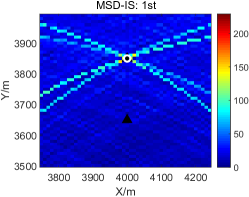
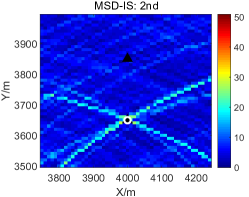
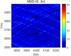
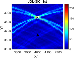
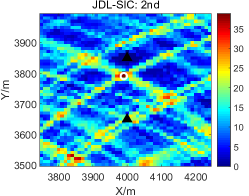
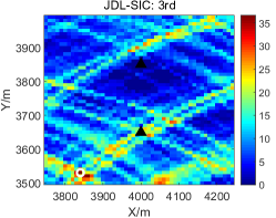
Figure 2: Output data planes of the MSD-IS (top) and JDL-SIC solutions (bottom) in three consecutive iterations (from left to right) when $\text{SNR}_{1}=13$ dB. The triangle markers are the true target positions; the circle marker is the estimated location of the target detected (if any) in each iteration.

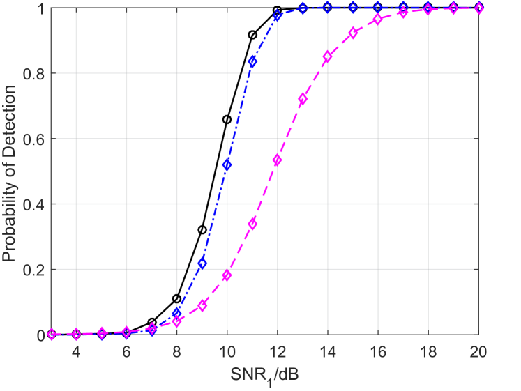
Figure 3: $\text{P}_{\text{d}}$ (left) and RMSE in the position estimate (right) of target $\text{Q}_{1}$ versus $\text{SNR}_{1}$.

We first compare the evolution of the MSD-IS and JDL-SIC solutions in a single snapshot. Fig. 2 reports the output data planes (i.e., the value of the scoring metric in the inspected region) over three iterations. It is verified that the MSD-IS is able to correctly detect and localize one target at the time during the first two iterations and that no additional target is found in the third one; in particular, the output data plane is progressively cleaned by the mitigation of the interference caused by the previously-detected (stronger) targets. In contrast, the JDL-SIC only performs well in the first iteration (wherein the strongest target is found), but fails in the subsequent ones. Finally, Fig. 3 reports $\text{P}_{\text{d}}$ and RMSE in the position estimate of target $\text{Q}_{1}$ versus $\text{SNR}_{1}$. It is seen that the MSD-IS performs close to the single-target benchmark, thus confirming its capability of detecting and localizing multiple targets even in the presence of a strong power imbalance among them. On the other hand, the performance of the JDL-SIC is not satisfactory, since this receiver is not able to properly handle the residual cross- and auto-terms in the MF output. Similar results have been obtained by including in the scene a larger number of targets, but the results have been omitted for brevity.

V Conclusions

This paper addresses the JDL of multiple targets in a distributed MIMO radar when the adopted waveforms present non-ideal cross- and auto-correlation properties. After modeling the data collected by each receiver as the noisy superposition of an unknown number of subspace signals, we have proposed to iteratively extract one target at the time by considering a sequence of composite binary hypothesis testing problems. Each testing problem has been solved via a generalized information criterion, thus resulting into a subspace-based detector which mitigates the cross- and auto-terms of the previously-detected targets via a zero-forcing transformation.

References

- [1] E. Fishler, A. Haimovich, R. S. Blum, L. J. Cimini, D. Chizhik, and R. A. Valenzuela, “Spatial diversity in radars—models and detection performance,” IEEE Transactions on signal processing, vol. 54, no. 3, pp. 823–838, Feb. 2006.
- [2] A. M. Haimovich, R. S. Blum, and L. J. Cimini, “MIMO radar with widely separated antennas,” IEEE Signal Processing Magazine, vol. 25, no. 1, pp. 116–129, Jan. 2007.
- [3] P. Wang, H. Li, and B. Himed, “Moving target detection using distributed MIMO radar in clutter with nonhomogeneous power,” IEEE Transactions on Signal Processing, vol. 59, no. 10, pp. 4809–4820, Jun. 2011.
- [4] A. Hassanien, S. A. Vorobyov, and A. B. Gershman, “Moving target parameters estimation in noncoherent MIMO radar systems,” IEEE Transactions on Signal Processing, vol. 60, no. 5, pp. 2354–2361, Feb. 2012.
- [5] M. Dianat, M. R. Taban, J. Dianat, and V. Sedighi, “Target localization using least squares estimation for MIMO radars with widely separated antennas,” IEEE Transactions on Aerospace and Electronic Systems, vol. 49, no. 4, pp. 2730–2741, Oct. 2013.
- [6] C.-H. Park and J.-H. Chang, “Closed-form localization for distributed MIMO radar systems using time delay measurements,” IEEE Transactions on Wireless Communications, vol. 15, no. 2, pp. 1480–1490, Oct. 2015.
- [7] R. Amiri, F. Behnia, and M. A. M. Sadr, “Exact solution for elliptic localization in distributed MIMO radar systems,” IEEE Transactions on Vehicular Technology, vol. 67, no. 2, pp. 1075–1086, Oct. 2017.
- [8] H. Godrich, A. M. Haimovich, and R. S. Blum, “Target localization accuracy gain in MIMO radar-based systems,” IEEE Transactions on Information Theory, vol. 56, no. 6, pp. 2783–2803, May 2010.
- [9] Q. He, R. S. Blum, and A. M. Haimovich, “Noncoherent MIMO radar for location and velocity estimation: More antennas means better performance,” IEEE Transactions on Signal Processing, vol. 58, no. 7, pp. 3661–3680, Mar. 2010.
- [10] O. Bar-Shalom and A. J. Weiss, “Direct positioning of stationary targets using MIMO radar,” Signal Processing, vol. 91, no. 10, pp. 2345–2358, Oct. 2011.
- [11] W. Yi, T. Zhou, Y. Ai, and R. S. Blum, “Suboptimal low complexity joint multi-target detection and localization for non-coherent MIMO radar with widely separated antennas,” IEEE Transactions on Signal Processing, vol. 68, pp. 901–916, 2020.
- [12] C. Ma, T. S. Yeo, C. S. Tan, Y. Qiang, and T. Zhang, “Receiver design for MIMO radar range sidelobes suppression,” IEEE Transactions on Signal Processing, vol. 58, no. 10, pp. 5469–5474, Oct. 2010.
- [13] Y. I. Abramovich and G. J. Frazer, “Bounds on the volume and height distributions for the MIMO radar ambiguity function,” IEEE Signal Processing Letters, vol. 15, pp. 505–508, 2008.
- [14] Y. Zhao, X. Lu, M. Ritchie, W. Su, and H. Gu, “Suppression of sidelobes in MIMO radar with distinctive piecewise non-linear frequency modulation sub-carrier,” International Journal of Remote Sensing, vol. 41, no. 1, pp. 353–372, Jul. 2019.
- [15] P. Wang and H. Li, “Target detection with imperfect waveform separation in distributed MIMO radar,” IEEE Transactions on Signal Processing, vol. 68, pp. 793–807, Jan. 2020.
- [16] H. Li, F. Wang, C. Zeng, and M. Govoni, “Signal detection in distributed MIMO radar with non-orthogonal waveforms and sync errors,” IEEE Transactions on Signal Processing, Jun. 2021.
- [17] C. Zeng, F. Wang, H. Li, and M. Govoni, “Delay compensation for distributed MIMO radar with non-orthogonal waveforms,” IEEE Signal Processing Letters, 2021.
- [18] E. Grossi, M. Lops, and L. Venturino, “An iterative interference cancellation algorithm for opportunistic sensing in ieee 802.11ad networks,” in IEEE 8th International Workshop on Computational Advances in Multi-Sensor Adaptive Processing, dec 2019, pp. 141–145.
- [19] E. Grossi, M. Lops, and L. Venturino, “Adaptive detection and localization exploiting the IEEE 802.11ad standard,” IEEE Transactions on Wireless Communications, vol. 19, no. 7, pp. 4394–4407, Mar. 2020.
- [20] E. Grossi, M. Lops, A. M. Tulino, and L. Venturino, “Extended target detection and localization in 802.11ad/y radars,” in 2020 IEEE Radar Conference, Sep. 2020.
- [21] E. Grossi, M. Lops, A. M. Tulino, and L. Venturino, “Opportunistic sensing using mmwave communication signals: a subspace approach,” IEEE Transactions on Wireless Communications, Feb. 2021.
- [22] F. Colone, C. Palmarini, T. Martelli, and E. Tilli, “Sliding extensive cancellation algorithm for disturbance removal in passive radar,” IEEE Transactions on Aerospace and Electronic Systems, vol. 52, no. 3, pp. 1309–1326, Jun. 2016.
- [23] G. Paolo Blasone, F. Colone, P. Lombardo, P. Wojaczek, and D. Cristallini, “Passive radar DPCA schemes with adaptive channel calibration,” IEEE Transactions on Aerospace and Electronic Systems, vol. 56, no. 5, pp. 4014–4034, Oct. 2020.
- [24] P. Stoica and Y. Selen, “Model-order selection: a review of information criterion rules,” IEEE Signal Processing Magazine, vol. 21, no. 4, pp. 36–47, Jul. 2004.
- [25] P. Stoica, Y. Selen, and J. Li, “On information criteria and the generalized likelihood ratio test of model order selection,” IEEE Signal Processing Letters, vol. 11, no. 10, pp. 794–797, Oct. 2004.