The 3D Galactocentric velocities of Kepler stars: marginalizing over missing RVs

Abstract

Precise Gaia measurements of positions, parallaxes, and proper motions provide an opportunity to calculate 3D positions and 2D velocities (i.e. 5D phase-space) of Milky Way stars. Where available, spectroscopic radial velocity (RV) measurements provide full 6D phase-space information, however there are now and will remain many stars without RV measurements. Without an RV it is not possible to directly calculate 3D stellar velocities, however one can infer 3D stellar velocities by marginalizing over the missing RV dimension. In this paper, we infer the 3D velocities of stars in the Kepler field in Cartesian Galactocentric coordinates ($v_{\bf x}$, $v_{\bf y}$, $v_{\bf z}$). We directly calculate velocities for around a quarter of all Kepler targets, using RV measurements available from the Gaia, LAMOST and APOGEE spectroscopic surveys. Using the velocity distributions of these stars as our prior, we infer velocities for the remaining three-quarters of the sample by marginalizing over the RV dimension. The median uncertainties on our inferred $v_{\bf x}$, $v_{\bf y}$, and $v_{\bf z}$ velocities are around 4, 18, and 4 kms^-1, respectively. We provide 3D velocities for a total of 148,590 stars in the Kepler field. These 3D velocities could enable kinematic age-dating, Milky Way stellar population studies, and other scientific studies using the benchmark sample of well-studied Kepler stars. Although the methodology used here is broadly applicable to targets across the sky, our prior is specifically constructed from and for the Kepler field. Care should be taken to use a suitable prior when extending this method to other parts of the Galaxy.

1 Introduction

Gaia has revolutionized the field of Galactic dynamics by providing positions, parallaxes and proper motions with unparalleled precision for a large number of Milky Way stars. So far, Gaia has provided positions, parallaxes and proper motions for around 1.7 billion stars, and radial velocities (RVs) for more than 7 million stars across its 1st, 2nd and early-3rd data releases (Gaia Collaboration et al., 2016, 2018, 2020). In combination, proper motion, position, and RV measurements provide full 6D phase-space information for any given star, which can be used to calculate its Galactic orbit. The orbits of stars are useful for kinematic age-dating, for exploring the secular dynamical evolution of the Galaxy, for differentiating between nascent and accreted stellar populations in the Milky Way’s halo, and many other applications.

One particular motivation is to use Galactic kinematics to study stellar evolution, either by using vertical velocity dispersion as an age proxy, or by calculating stellar ages via an age-velocity dispersion relation (e.g. Angus et al., 2020; Lu et al., 2021). The ages of stars, particularly GKM stars on the main sequence, are difficult to measure because their luminosities and temperatures evolve slowly (see Soderblom, 2010, for a review of stellar ages). Galactic kinematics provides an alternative, statistical dating method.

Older populations of stars are observed to have larger velocity dispersions than younger populations, and this is generally thought to be caused by dynamical heating of the Galactic disc by giant molecular clouds and spiral arms (e.g. Strömberg, 1946; Wielen, 1977; Nordström et al., 2004; Holmberg et al., 2007, 2009; Aumer & Binney, 2009; Casagrande et al., 2011; Yu & Liu, 2018; Ting & Rix, 2019). This behavior is codified by empirically-calibrated Age-Velocity dispersion Relations (AVRs), which typically express the relationship between age and velocity dispersion as a power law: $\sigma_{v}\propto t^{\beta}$, with free parameter, $\beta$ (e.g. Holmberg et al., 2009; Yu & Liu, 2018; Mackereth et al., 2019). These expressions can be used to calculate the ages of stellar populations from their velocity dispersions. However, AVRs are usually calibrated in 3D Galactocentric velocities, and most commonly in vertical velocity: $v_{\bf z}$ or W. Regardless of the coordinate system, some transformation from RV and proper motion in equatorial coordinates is usually required to calculate the kinematic ages of stars using an AVR.

RV measurements, combined with positions, parallaxes, and proper motions measured in the plane of the sky, complete the full set of information needed to calculate 3D stellar velocities. However, RV generally has to be measured from a stellar spectrum – an observation that requires a significant number of photons and is thus expensive to obtain, particularly for faint stars . Fortunately however, the bulk circular velocity of the Galactic disc allows stellar velocities to be inferred by using an informative prior that is constructed from the velocities of stars with full 6D phase-space information. This will often result in a velocity that is not equally well-constrained in every direction, i.e. the probability density function of a star’s velocity will be an oblate spheroid in 3D. In the equatorial coordinate system, a star’s velocity will be tightly constrained in the directions of RA and dec, and only constrained by the prior in the radial direction. Transforming to any other coordinate system, a star’s velocity probability density function will change shape via a transformation that depends on its position.

In this work, we provide 3D velocities in $v_{\bf x}$, $v_{\bf y}$, and $v_{\bf z}$ for Kepler targets. Our motivation is chiefly to calculate vertical velocities ($v_{\bf z}$) which can then be used to calculate the ages of stellar populations via an AVR, from which other empirical age-dating methods can be calibrated. For example, empirical or semi-empirical models that relate the magnetic activity or rotation periods of stars to their age can be used to infer the ages of some low-mass dwarfs (e.g. Skumanich, 1972; Barnes, 2003, 2007; Mamajek & Hillenbrand, 2008; Matt et al., 2012; Angus et al., 2019; Claytor et al., 2020), however, these empirical relations are often poorly calibrated for low-mass and old stars (e.g. Angus et al., 2015; van Saders et al., 2016, 2018; Metcalfe & Egeland, 2019; Curtis et al., 2020; Spada & Lanzafame, 2019; Angus et al., 2020). In Angus et al. (2020) we used the velocities of Kepler stars in the direction of Galactic latitude, $v_{\bf b}$  as a proxy for vertical velocity. $v_{\bf b}$ can be calculated without an RV and it is similar to $v_{\bf z}$ for many Kepler stars because the Kepler field lies at low Galactic latitude. We used the $v_{\bf b}$ velocity dispersions of stars as an age proxy to explore the evolution of stellar rotation rates. In Lu et al. (2021) we used vertical velocity dispersion ($v_{\bf z}$) to calculate kinematic ages for Kepler stars with measured rotation periods using an age-velocity dispersion relation (AVR). Those vertical velocities were inferred by marginalizing over missing RVs using the method we describe in this paper. To expand upon that work and provide an opportunity to apply kinematic age-dating to more stars, we here calculate the 3D velocities of all Kepler targets. Although we focus on the Kepler field, the methodology presented in this paper is applicable to stars across the sky if a suitable prior is used.

There are several other applications for which the 3D velocity of a star is useful, even if its velocity is not equally well-constrained in every direction. For example, Oh et al. (2017) used Gaia proper motions to identify comoving pairs and groups of stars by marginalizing over missing RVs. In their study, the relative space motions of pairs of stars were used to establish whether they qualified as ‘comoving’. In a pathological case where two stars (nearby on the sky) have near identical proper motions and completely different RVs, their method would incorrectly flag them as comoving stars, however in general the Gaia proper motion precision is sufficiently high to make these cases rare.

Another work that predicts 3D velocities of Gaia targets is Dropulic et al. (2021), in which the velocities of mock Gaia stars are predicted with a neural network. The network is trained on the velocities of stars with RVs and used to predict the velocities of stars without. The method we present here seeks to solve the same problem via a different methodology: we use Bayesian inference instead of a neural network. It is difficult to draw a direct comparison between their method and ours because we use different coordinate systems (we use Cartesian, and they use cylindrical coordinates), and because we focus on different populations – they predict velocities for the entire Gaia catalog, whereas we concentrate on a small part of the sky. The two approaches will be useful for different scientific applications, and it is extremely useful to have multiple approaches to solving this fundamental problem in astronomy.

It is worth noting that ignoring the RV dimension and attempting to calculate stellar velocities with proper motions and distances alone, i.e. assuming that RV can be set to zero, will introduce a significant bias in the resulting velocities. We explore this point further in section 4.

This paper is laid out as follows. In section 2 we describe the data used in this paper. In section 3 we describe how we calculate the kinematic ages of Kepler stars from their positions, proper motions and parallaxes, marginalizing over missing RVs. We also justify the choice of prior probability density function (PDF). In section 4 we present the 3D velocities of a subsample of the total 148,590 Kepler stars and explore the accuracy and precision of our method.

2 The Data

We used the Kepler-Gaia cross-matched catalog that is available at https://gaia-kepler.fun. This catalog contains 198,451 Kepler targets, cross-matched with Gaia targets within in a 1” radius and includes positions, parallaxes, and proper motions from Gaia EDR3 and RVs from Gaia DR2. We crossmatched this catalog with the catalog of photogeometric distances inferred from Gaia EDR3 parallaxes (Bailer-Jones et al., 2021) and applied corrections to EDR3 parallaxes based on Lindegren et al. (2021). We also crossmatched this catalog with the LAMOST DR5 catalog and the APOGEE DR16 stellar catalog (Cui et al., 2012; Ahumada et al., 2020; Xiang et al., 2019). We removed stars with angular separations larger than 150 milliarcseconds during each of these crossmatches. Stars with effective temperatures that differed by more than 500K between Gaia, APOGEE, and LAMOST were removed from the sample to minimize incorrect crossmatches. To remove stars with multiple crossmatches within 150 milliarcseconds, we only kept the star with the smallest angular separation. We also removed stars with a Gaia parallax $<$ 0, parallax signal-to-noise ratio $<$ 10, and Gaia astrometric excess noise $>$ 5. To preferentially select single stars, we removed stars with ruwe $\geq$ 1.4, ipd_frac_multi_peak $>2$, and ipd_gof_harmonic_amplitude $\geq$ 0.1. APOGEE reports VSCATTER, which is the error-deconvolved scatter in the individual time-series RV measurements for each source and can indicate that a star is a binary. We removed 208 stars in our final sample with APOGEE VSCATTER greater than 1 km s^-1. After applying these cuts our total number of targets was 148,590. In total, 38,884 stars in our sample have at least one RV measurement from Gaia, LAMOST, or APOGEE; 23,013 have RVs from Gaia DR2, 22,420 from LAMOST DR5, and 7,697 from APOGEE DR16. The APOGEE survey (R $=$ 22,500; Majewski et al., 2017) has a higher spectral resolution than Gaia (R $=$ 11,500; Cropper et al., 2018), which in turn is higher than LAMOST (R $=$ 1,800; Zhao et al., 2012). The median RV uncertainty for stars in our sample is around 0.1 km/s for APOGEE RVs, 1 km/s for Gaia RVS, and 5 km/s for LAMOST RVs. In cases where stars had two or more available RV measurements, we adopted APOGEE RVs as a first priority, followed by Gaia, then LAMOST.

Although RVs are available for more than one in three Kepler targets, most stars with RV measurements are bright. Very few of the faintest stars have RVs because of the selection functions of spectroscopic surveys. Most of the stars in our sample with Gaia RV measurements are brighter than around 14th magnitude in Gaia $G$-band, and stars with LAMOST or APOGEE RVs are mostly brighter than around 16th magnitude. Figure 1 shows the apparent magnitude distributions of the stars in our sample, with and without RVs. This figure reveals the combined selection functions of the Gaia, LAMOST and APOGEE RV surveys and shows that faint stars are less likely to have RV measurements than bright ones.

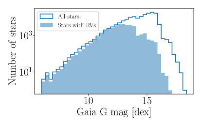
Figure 1: The distribution of apparent Gaia magnitudes for stars in our sample with and without RV measurements from Gaia, LAMOST and APOGEE.

To illustrate how the populations of stars with and without RVs differ, we plot them on a color-magnitude diagram (CMD) in figure 2. The stars with RVs are generally hotter and more luminous than stars without. Most stars with RVs fall on the upper main sequence, the red giant branch, and the red clump. Most stars without RVs fall on the main sequence. This overall selection function is a combination of the APOGEE, LAMOST and Gaia DR2 selection functions.

In this paper, we construct a prior using stars with RV measurements which we then use to infer the velocities of stars without RV measurements. However, given that the populations of stars with and without RVs are so different, this could bias the velocities we infer, particularly if they are prior-dependent. We investigate this idea in section 3.2 and find that the $v_{\bf x}$ and $v_{\bf z}$ velocities we infer are relatively insensitive to the prior and therefore unlikely to biased, however the $v_{\bf y}$ velocities we infer should be used with caution as they are relatively prior-dependent.

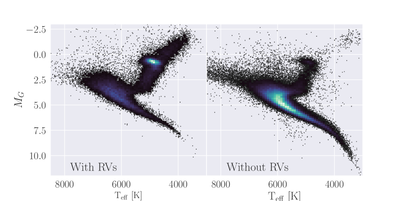
Figure 2: A magnitude-temperature diagram of stars in the Kepler field with (left) and without (right) RVs provided by Gaia, LAMOST and APOGEE. The stars with RVs are generally hotter and more luminous than those without RVs, and include a large number of red clump stars and red giant branch stars. Stars without RVs are mostly concentrated on the main sequence.

3 Method

In this section we describe how we calculate full 3D velocities for stars in the Kepler field. Around 1 in 3 Kepler targets have an RV from either Gaia, LAMOST, or APOGEE. For these 38,884 stars we calculated 3D velocities using the coordinates library of astropy (Astropy Collaboration et al., 2013; Price-Whelan et al., 2018). This library performs a series of matrix rotations and translations to convert stellar positions and velocities in equatorial coordinates into positions and velocities in Galactocentric coordinates. It converts positions, proper motions, parallaxes/distances, and RVs into ${\bf x}$, ${\bf y}$, ${\bf z}$, $v_{\bf x}$, $v_{\bf y}$, $v_{\bf z}$. We adopted a Solar position of $r_{\odot}=8.122$ kpc (Gravity Collaboration et al., 2018) and $z_{\odot}=20.8$ pc (Bennett & Bovy, 2019), and a Solar velocity of $v\odot=(12.9,245.6,7.78)$ km s^-1(Drimmel & Poggio, 2018). For stars without RVs, we inferred their velocities by marginalizing over their RVs using the method described below.

3.1 Inferring 3D velocities (marginalizing over missing RV measurements)

For each star in our sample without an RV measurement, we inferred $v_{\bf x}$, $v_{\bf y}$, and $v_{\bf z}$ from the 3D positions – RA ($\alpha$), dec ($\delta$), and parallax ($\pi$), and 2D proper motions ($\mu_{\alpha}$ and $\mu_{\delta}$) provided in the Gaia EDR3 catalog (Gaia Collaboration et al., 2020). We also simultaneously inferred distance (instead of using inverse-parallax) to model velocities (see e.g. Bailer-Jones, 2015; Bailer-Jones et al., 2018).

Using Bayes rule, the posterior probability of the velocity parameters given the Gaia data can be written:

$$p({\bf v_{xyz}},D|\mu_{\alpha},\mu_{\delta},\alpha,\delta,\pi)=p(\mu_{\alpha},\mu_{\delta},\alpha,\delta,\pi|{\bf v_{xyz}},D)p({\bf v_{xyz}})p(D),$$ (1)

where $D$ is distance and ${\bf v_{xyz}}$ is the 3D vector of velocities. To evaluate the likelihood function, our model predicts observable data from model parameters, i.e. it converts $v_{\bf x}$, $v_{\bf y}$  $v_{\bf z}$ and $D$ to $\mu_{\alpha}$, $\mu_{\delta}$ and $\pi$. In the first step of the model evaluation, cartesian coordinates, ${\bf x}$, ${\bf y}$, and ${\bf z}$  are calculated from $\alpha$, $\delta$, and $D$ by applying a series of matrix rotations, and a translation to account for the Solar position. The cartesian Galactocentric velocity parameters, $v_{\bf x}$, $v_{\bf y}$, and $v_{\bf z}$, are then converted to equatorial coordinates, $\mu_{\alpha}$ and $\mu_{\delta}$ via another rotation. The posterior PDFs of the parameters $v_{\bf x}$, $v_{\bf y}$, $v_{\bf z}$, and $\ln(D)$ are sampled by evaluating this model over a range of parameter values which are chosen by via the No U-Turns Sampler (NUTS) algorithm in PyMC3. At each set of model parameters the likelihood is calculated via a Gaussian likelihood function, and multiplied by a prior (described below) to produce the posterior probability: the probability of those model parameters given the data.

For computational efficiency, we used PyMC3 to sample the posterior PDFs of stellar velocities (Salvatier et al., 2016). This required that we rewrite the astropy coordinate transformation code using numpy and Theano (Harris et al., 2020; The Theano Development Team et al., 2016). The series of rotations and translations required to convert from equatorial to Galactocentric coordinates is described in the astropy documentation (Price-Whelan et al., 2018). For each star in the Kepler field, we explored the posteriors of the four parameters, $v_{\bf x}$, $v_{\bf y}$, $v_{\bf z}$, and $\ln(D)$ using the PyMC3 No U-Turn Sampler (NUTS) algorithm, and the exoplanet Python library (Foreman-Mackey & Barentsen, 2019). We tuned the PyMC3 sampler for 1500 steps, with a target acceptance fraction of 0.9, then ran four chains of 1000 steps for a total of 4000 steps. This resulted in a $\hat{r}$-statistic (the ratio of intra-chain to inter-chain variance) of around unity, indicating convergence. Using PyMC3 made this inference procedure exceptionally fast – taking just a few seconds per star on a laptop.

3.2 The prior

As mentioned previously, the positioning of the Kepler field at low Galactic latitude allows $v_{\bf z}$ to be well-constrained from proper motion measurements alone. This also happens to be the case for $v_{\bf x}$, because the direction of the Kepler field is almost aligned with the ${\bf y}$-axis of the Galactocentric coordinate system and is almost perpendicular to both the ${\bf x}$ and ${\bf z}$-axes (see figure 3). For this reason, the ${\bf y}$-direction is similar to the radial direction for observers near the Sun, so $v_{\bf y}$ will be poorly constrained for Kepler stars without RV measurements. On the other hand, $v_{\bf x}$ and $v_{\bf z}$ are almost perpendicular to the radial direction and can be precisely inferred with proper motions alone.

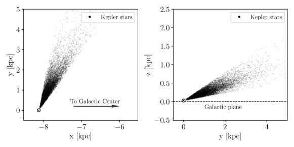
Figure 3: ${\bf x}$, ${\bf y}$ and ${\bf z}$ positions of stars observed by Kepler, showing the orientation of the Kepler field. The Sun’s position is indicated with a Solar symbol. The direction of the field is almost aligned with the ${\bf y}$-axis and almost perpendicular to the ${\bf x}$ and ${\bf z}$-axes, which is why $v_{\bf x}$ and $v_{\bf z}$ can be tightly constrained for Kepler stars without RVs, but $v_{\bf y}$ cannot.

We constructed a multivariate Gaussian prior PDF over distance and 3D velocity using the Kepler targets which have RV measurements. We calculated the means and covariances of the $v_{\bf x}$, $v_{\bf y}$, $v_{\bf z}$ and $\ln(D)$ distributions of stars with measured RVs and then used these means and covariances to construct a multivariate Gaussian prior over the velocity and distance parameters for stars without RVs. Velocity and distance outliers greater than 3-$\sigma$ were removed before calculating the means and covariances of the distributions. The distance and velocity distributions of Kepler targets with RVs are displayed in figure 4. These are the distributions we used to construct the prior. The 1- and 2-$\sigma$ contours of the multivariate Gaussian prior is shown in each panel in red. This figure shows that Gaussian functions only approximately reproduce the true velocity distributions, and do not capture the substructure. We could have chosen a more complex prior that would fit these data better, for example, a mixture of Gaussians, which would capture the moving groups in the Solar neighborhood. This may result in slightly more accurate inferred velocities. However, since our goal is kinematic age dating, we only need to resolve the vertical velocity component to a sufficient precision that will accurately allow for calculations of vertical velocity dispersions, so the minor gain in precision will not have a large affect on the end results. In addition, since this prior is constructed using stars with RVs, which may have a slightly different velocity distribution to stars without RVs, we opted for the more uninformative, simple Gaussian prior.

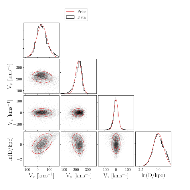
Figure 4: The velocity and distance distributions for stars with RV measurements, used to construct a multivariate Gaussian prior over velocity and distance parameters for stars without RVs. The 1- and 2-D distributions of the data are shown in black and the prior is indicated in red.

Our goal was to infer the velocities of stars without RV measurements using a prior calculated from stars with RV measurements. However, stars with and without RVs are likely to be quite different populations, determined by the Gaia, LAMOST and APOGEE selection functions. In particular, stars without RV measurements are more likely to be fainter, less luminous, cooler and potentially older. Figure 2 shows the populations of stars with and without RVs on the CMD – stars with RVs are more likely to be upper-main-sequence and red giant stars, and stars without RVs are more likely to be mid and lower main-sequence dwarfs. For this reason, a prior based on the velocity distributions of stars with RVs will not necessarily reflect the velocities of those without. We could have opted to construct a prior that depends on CMD position, however, in practice, this would require making a number of arbitrary choices, so we instead opted for a simpler approach. In addition, we find that the $v_{\bf x}$ and $v_{\bf z}$ velocities we infer are not strongly influenced by the prior, as described below.

We tested the influence of the prior on the velocities we inferred. One of the main features of the RV selection functions is brightness: Gaia DR2 RVs are only available for stars brighter than around 14th magnitude, and LAMOST DR5 and APOGEE DR16 RVs for stars brighter than around 16th magnitude. For this reason, we tested priors based on stellar populations with different apparent magnitudes. Three priors were tested: one calculated from the velocity distributions of the brightest half of the RV sample (Gaia $G$-band apparent magnitude $<$ 13), one from the faintest half ($G$ $>$ 13), and one from all stars with RVs. Figure 5 shows the distributions of the faint (blue) and bright (orange) halves of the RV sample as kernel density estimates (KDEs). The distributions are different because bright stars are typically more massive, younger, more evolved, and/or closer to the Sun on average than faint stars. As a result, these stars occupy slightly different Galactic orbits. The multivariate Gaussian, fit to these distributions, which was used as a prior PDF, is shown as single-dimension projections in figure 5. The Gaussian fit to the bright and faint star distributions are shown as dashed orange and blue lines, respectively. The Gaussian fit to all the data, both bright and faint, is shown as a black solid line. The means of the faint and bright distributions differ by 6 km s^-1, 5 km s^-1, 1 km s^-1 and 0.21 kpc, for $v_{\bf x}$  $v_{\bf y}$, $v_{\bf z}$ and $\ln(D)$, respectively. The $v_{\bf x}$, $v_{\bf y}$, and distance distributions of the bright stars are slightly non-Gaussian – more so than the faint stars. This highlights the inadequacy of using a Gaussian distribution as the prior – a Gaussian is only an approximation of the underlying distribution of stars in our sample. As a result of this approximation, inferred velocities that are strongly prior-dependent – (i.e. especially those in the ${\bf y}$-direction) may inherit some inaccuracies from the Gaussian prior, which is not a perfect representation of the underlying data. However, given that the populations of stars with and without RV measurements are different, it may be inappropriate to use a more complex, more informative prior anyway.

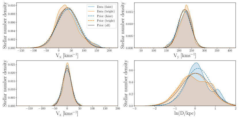
Figure 5: Velocity and distance distributions of faint (blue) and bright (orange) stars with RVs, shown as KDEs. Gaussian fits to these distributions are shown as dashed lines in corresponding colors. The solid black line shows the Gaussian fit to all data (bright and faint combined) and is the prior we ended up using in our model. This figure highlights the differences between the velocities and distances of bright and faint stars (with RVs) in our sample.

We inferred the velocities of 1000 stars chosen at random from the RV Kepler sample using each of these three priors and compared the inferred velocity distributions. If the inferred velocities were highly prior-dependent, the resulting distributions, obtained from different priors, would look very different. The results of this test are shown in figure 6. From left to right, the three panels show the distributions of inferred $v_{\bf x}$, $v_{\bf y}$, $v_{\bf z}$, and log-distance. The blue dashed line shows a KDE representing the distributions of velocities inferred using the prior calculated from the faint half of the RV sample. Similarly, the solid orange line shows the distribution of inferred velocities using the prior calculated from the bright half of the RV sample, and the solid black line shows the results of the prior calculated from all stars with measured RVs. In all but the $v_{\bf y}$ panel (second from the left), the blue, orange, and black lines lie on top of each other, indicating that different priors do not significantly influence the resulting velocities.

The median values of the $v_{\bf y}$ distributions resulting from the faint and bright priors differ by around 4 km s^-1. This is similar to the difference in means of the faint and bright populations (5 km s^-1, as quoted above). The inferred $v_{\bf x}$ and $v_{\bf z}$ distributions differ by 2 km s^-1 and 0.3 km s^-1, respectively. Regardless of the prior choice, the $v_{\bf x}$ and $v_{\bf z}$ distributions are similar because velocities in the ${\bf x}$ and ${\bf z}$-directions are not strongly prior dependent: they are tightly constrained with proper motion measurements alone. However, the distribution of inferred $v_{\bf y}$ velocities does depend on the prior. This is because the ${\bf y}$-direction is close to the radial direction for Kepler stars (see figure 3), and $v_{\bf y}$ cannot be tightly constrained without an RV measurement. The distributions of stellar distances are almost identical, irrespective of the prior. This is because distance is very tightly constrained by Gaia parallax and is relatively insensitive to the prior.

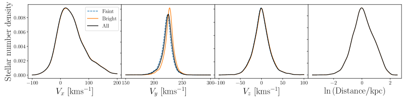
Figure 6: The distributions of velocity and distance parameters, inferred using three different priors. The orange line is a KDE that represents the distribution of parameters inferred with a Gaussian prior, estimated from the bright half of the RV sample ($G<$ 13). The blue dashed line shows the results from a prior estimated from the faint half of the RV sample ($G>13$)). The black line shows the results from a prior calculated from all stars with RV measurements and is the prior we adopt in our final analysis. This figure shows that all parameters except $v_{\bf y}$ are relatively insensitive to the three priors that were tested.

Although this test was performed on stars with RV measurements, which are brighter overall than the sample of stars without RVs (e.g. figure 1), figure 6 nevertheless indicates that $v_{\bf x}$ and $v_{\bf z}$ are not strongly prior-dependent. Since this work is chiefly motivated by kinematic age-dating, which mostly requires vertical velocities ($v_{\bf z}$), we are satisfied with these results. We conclude that the $v_{\bf x}$ and $v_{\bf z}$ velocities we infer are relatively insensitive to prior choice, and we adopt a prior calculated from the distributions of all stars with RV measurements (black Gaussians in figure 5). The $v_{\bf y}$ velocities are more strongly prior dependent and should be used with caution.

A better prior for the velocity distribution would be a phase-space distribution function that takes into account asymmetric drift and other nontrivial aspects of the local velocity distribution. However, priors of this form would require a model for the phase-space distribution function, $f(x,y,z,v_{x},v_{y},v_{z})$, which would require a hierarchical model that takes into account covariances between the spatial and kinematic properties of stars (e.g. Trick et al., 2016; Hagen et al., 2019; Anguiano et al., 2020). We consider this to be outside of the scope of this work, and instead argue that our assumed isotropic velocity prior is a conservative choice because it does not impose any covariant structure between velocity components or dependencies on Galactic position. However, in general, to extend this Kepler-field-specific analysis to other populations of stars in different parts of the Galaxy, alternative priors will have to be constructed. We leave this for a future exercise.

Figure 7 shows the posterior PDF over velocity and distance parameters for a randomly selected Kepler target with an RV measurement, KIC 12218729. The blue lines in each panel indicate star’s velocities, directly calculated using the RV measurement, and the distributions indicate the probability density of the parameters inferred without the RV measurement. The velocity parameters are correlated because the lack of RV introduces a slight degeneracy: the star’s proper motion can be equally well described with a range of different velocities. The star’s posterior PDF is particularly elongated in $v_{\bf y}$, which is the velocity most similar to RV. The star’s distance is not tightly correlated with its velocity parameters because it is precisely determined by parallax.

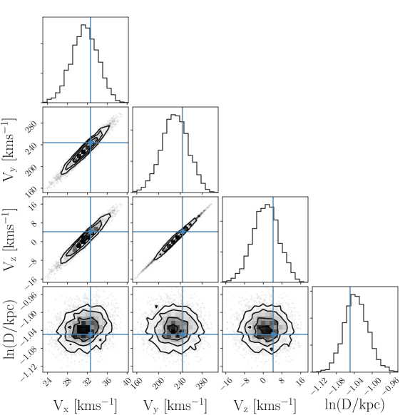
Figure 7: The posterior PDF over parameters $v_{\bf x}$, $v_{\bf y}$, $v_{\bf z}$ and $\ln$(distance) for a Kepler target chosen at random: KIC 12218729. Blue lines show the location of the star’s ‘true’ parameters, based on a calculation that includes the RV measurement. This figure shows that the velocity parameters are correlated and the star’s posterior is elongated in $v_{\bf y}$.

4 Results and Discussion

4.1 Inferred velocities

In this section we assess the quality of the 3D stellar velocities we infer. Figure 8 shows the distribution of stellar velocities inferred for 5000 randomly selected Kepler stars. The 2D distributions of inferred stellar velocities are plotted in the lower-left panels, with black contours indicating the stellar number density. The red contours in these panels show the marginal projections of the Gaussian prior in 2D. The diagonal panels show the 1D distributions (histograms) of stellar velocities. The black histogram shows the distribution of inferred velocities, the cyan histogram shows the distribution of velocities calculated for stars with RVs (on which the prior was based), and the red lines show the 1D prior distributions. The prior distribution was calculated using the velocities of stars with RVs. If the velocity distributions of stars were Gaussian, the 1D red Gaussians would look like the cyan histograms. In other words, the differences between the red lines and cyan histograms is caused by the non-Gaussianity of the velocity distributions. This figure is intended to highlight the differences and similarities between the inferred stellar velocities and the prior distributions. In each panel, the distribution of inferred velocities is fairly similar to the distribution of directly-measured velocities; the velocities of stars calculated with and without RVs are broadly similar. The inferred $v_{\bf x}$ and $v_{\bf z}$ velocities, and distances are relatively precise, with median uncertainties of 4km s^-1, 4 km s^-1, and 1 kpc, respectively. The inferred $v_{\bf y}$ velocities have a median uncertainty of 18 km s^-1.

There is a slight negative correlation between inferred $v_{\bf y}$ and $v_{\bf z}$ velocities, which is visible in the central panel of figure 8. This negative correlation is not seen in the prior, nor is it apparent in the posteriors of individual stars: figure 7 shows that the $v_{\bf y}$ and $v_{\bf z}$ parameters are positively correlated for KIC 12218729. This negative correlation may be due to the specific orientation of the Kepler field, which creates a slight degeneracy between $v_{\bf y}$ and $v_{\bf z}$. If this explanation is correct, this phenomenon highlights how apparent correlations in stellar velocities could result from missing information. This point is interesting, but the effect is relatively small and we do not expect that this observed correlation between $v_{\bf z}$ and $v_{\bf y}$ will significantly affect kinematic age studies.

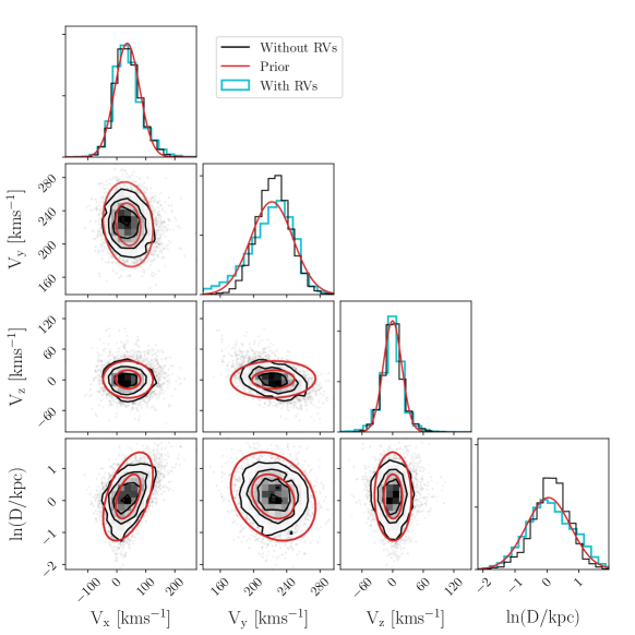
Figure 8: The distribution of inferred stellar velocities and distances. Figure 8 shows the inferred velocities of 5000 randomly selected Kepler stars. The 2D distributions of inferred stellar velocities are plotted in the lower-left panels, with black contours indicating the stellar number density. The red contours in the lower-left panels show the marginal projections of the Gaussian prior distribution in 2D. The upper-right panels in the figure, lying on the plot’s diagonal, show the 1D distributions (histograms) of stellar velocities. The black histogram shows the distribution of inferred velocities, the blue histogram shows the distribution of velocities for stars with RVs, and the red lines show the 1D marginal Gaussian prior distributions. This figure shows that the distributions of inferred velocities are broadly similar to the distributions of velocities directly calculated using RVs, and the prior constructed from them.

To further validate our method, we compare inferred velocities with directly-calculated velocities for stars in our sample with measured RVs. Figure 9 shows the $v_{\bf x}$, $v_{\bf y}$ and $v_{\bf z}$ velocities, and distances we inferred, compared with those calculated from measured RVs, for 5000 Kepler stars chosen at random.

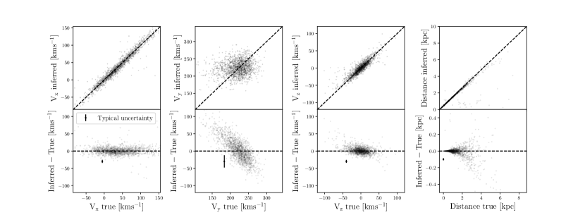
Figure 9: Velocities calculated with full 6D information compared with velocities inferred without RVs, for 5000 Kepler targets with RV measurements.

The three velocity components, $v_{\bf x}$, $v_{\bf y}$ and $v_{\bf z}$ were recovered with differing levels of precision: $v_{\bf x}$ and $v_{\bf z}$ are inferred more precisely than $v_{\bf y}$. This is because of the position of the Kepler field, shown in figure 3. The velocities of low-$v_{\bf y}$ stars are overestimated and the velocities of high-$v_{\bf y}$ stars are underestimated. This is because there is little information to constrain the $v_{\bf y}$ velocities and the prior pulls the $v_{\bf y}$ velocities toward the center of the distribution. The $v_{\bf x}$, $v_{\bf y}$ and $v_{\bf z}$ velocities of stars are correlated, which means that stars with an inaccurate $v_{\bf y}$ also have slightly accurate $v_{\bf z}$ and $v_{\bf x}$. Despite slight systematic inaccuracies visible in the residual (bottom) panels of figure 9, around 68% of the inferred velocities are within 1$\sigma$ of their true velocities; the inferred velocities are consistent with the true velocities.

We provide a table of the directly-calculated, and indirectly-inferred 3D velocities of stars observed by Kepler, in addition to their positional and velocity information from Gaia EDR3, LAMOST DR5 and APOGEE DR16. A description of each column included in that table is provided in table 1.

As briefly mentioned in the introduction, we have gone to the trouble of inferring velocities in this paper because calculating velocities from proper motions and distances alone, i.e. assuming the RV is zero, will bias the resulting velocities. To demonstrate this, figure 10 shows the velocity residuals for stars in our sample where we infer the velocities by marginalizing over RV and where we ignore RV, i.e. set it to zero. In each panel, the green distributions show the residuals between the true velocities and our inferred velocities, and the purple distributions show the residuals between the true velocities and velocities calculated by setting the RV to zero. The median of each distribution is shown as a vertical line. This figure shows that ignoring the RV dimension and assuming it can be set to zero significantly biases the resulting velocities. The correct way to de-bias velocity calculations is to marginalize over missing RV measurements.

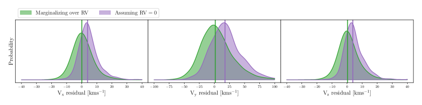
Figure 10: Residual velocity distributions calculated by marginalizing over missing RV measurements (green) or by assuming the RV can be set to zero (purple) for 5000 stars in our sample. Each distribution shows the residuals between the inferred/calculated velocities, and the velocities calculated using full 6D information: parallaxes, positions, proper motions, and RVs. The vertical lines show the medians of each distribution. This figure demonstrates that calculating stellar velocities using proper motions and distances alone will significantly bias the results. Marginalizing over missing RV measurements ensures the resulting velocities will be unbiased.

Our intention in providing a table of stellar velocities, and outlining our method for inferring velocities without RV measurements, is to facilitate kinematic age-dating studies. The vertical velocities we provide could be used as an age proxy, or to calculate kinematic ages via an age-velocity dispersion relation (e.g. Yu & Liu, 2018; Mackereth et al., 2019; Sharma et al., 2021). This kind of approach has been used many times to examine the kinematic ages of cool stars to explore stellar and planetary evolution (e.g. Newton et al., 2016; Kiman et al., 2019; Hamer & Schlaufman, 2019; Angus et al., 2020; Lu et al., 2021). For example, Kiman et al. (2019) used the vertical velocity dispersions of stars as an age proxy to explore the evolution of H$\alpha$ equivalent width (a magnetic activity indicator), in M dwarfs. Hamer & Schlaufman (2019) compared the vertical velocity dispersions of stars with and without hot Jupiters to show that hot Jupiter hosts tend to be younger, on average, than stars without detected hot Jupiters.

Table 1: The list of columns in the data table published online, which provides the velocities and kinematic information for stars in the Kepler field.

Column name	Description
KIC	The Kepler Input Catalog ID number of the target.
Gaia	The Gaia DR3 source ID of the target.
RAdeg, e$\_$RAdeg	Gaia EDR3 right ascenscion (∘).
DEdeg, e$\_$DEdeg	Gaia EDR3 declination in degrees (∘).
plx, e$\_$plx	Gaia EDR3 parallax (mas).
Dist, b$\_$Dist, B$\_$Dist	Distance, lower and upper bounds (parsec), provided by Bailer-Jones et al. (2021).
pmRA, e$\_$pmRA	Gaia EDR3 proper motion in right ascension (mas/yr).
pmDE, e$\_$pmDE	Gaia EDR3 proper motion in declination (mas/yr).
RV-gaiaDR2, e$\_$RV-gaiaDR2	Gaia DR2 radial velocity (km/s)
RV-apo16, e$\_$RV-apo16	APOGEE DR16 radial velocity (km/s)
RV-lamDR5, e$\_$RV-lamDR5	LAMOST DR5 radial velocity (km/s)
vx-calc	The $v_{\bf x}$ velocity calculated using RV (km/s).
vx-inferred, e$\_$vx-inferred	Median and std. dev, of $v_{\bf x}$ velocity samples, inferred without RV (km/s).
vy-calc	The $v_{\bf y}$ velocity calculated using RV (km/s).
vy-inferred, e$\_$vy-inferred	Median and std. dev. of $v_{\bf y}$ velocity samples, inferred without RV (km/s).
vz-calc	The $v_{\bf z}$ velocity calculated using RV (km/s).
vz-inferred, e$\_$vz-inferred	Median and std. devi. of $v_{\bf z}$ velocity samples, inferred without RV (km/s).
vxvy-covar	The covariance between $v_{\bf x}$ and $v_{\bf y}$ samples.
vxvz-covar	The covariance between $v_{\bf x}$ and $v_{\bf z}$ samples.
vxlnd-covar	The covariance between $v_{\bf x}$ and $\ln$(distance) samples.
vyvz-covar	The covariance between $v_{\bf y}$ and $v_{\bf z}$ samples.
vylnd-covar	The covariance between $v_{\bf y}$ and $\ln$(distance) samples.
vzlnd-covar	The covariance between $v_{\bf z}$ and $\ln$(distance) samples.

5 Conclusion

This paper describes a method for inferring the 3D velocities of stars by marginalizing over missing radial velocity measurements. We focused on stars in the Kepler field because of its potential for studying stellar evolution via kinematic age-dating as well as its advantageous orientation. Located at low Galactic latitude, the Kepler field is almost aligned with the $y$-axis of the Galactocentric coordinate system. This means that 2D Gaia proper motion measurements alone are sufficient to tightly constrain the $v_{\bf x}$ and $v_{\bf z}$ velocities of Kepler stars. Without RV measurements, the $v_{\bf y}$ velocities of Kepler stars are poorly constrained. However, given that many age-velocity dispersion relations (AVR) are calibrated in vertical velocity, $v_{\bf z}$ is the main parameter of interest for kinematic age-dating and it is precisely constrained by our method: $v_{\bf z}$ is inferred with a median precision of 4 kms^-1.

We compiled kinematic data for Kepler targets from the, Gaia EDR3, LAMOST DR5 and APOGEE DR16 catalogs. Gaia EDR3 provided parallaxes, positions and proper motions for the stars in our sample. Altogether, Gaia DR2, LAMOST DR5, and APOGEE DR16 provided RVs for 38,884 Kepler targets.

We calculated $v_{\bf x}$, $v_{\bf y}$, and $v_{\bf z}$ for the 38,884 stars in our sample with RVs using astropy. For the remaining stars, we inferred $v_{\bf x}$, $v_{\bf y}$, $v_{\bf z}$, and distance while marginalizing over RV. Our prior was a 4D Gaussian in $v_{\bf x}$, $v_{\bf y}$, $v_{\bf z}$ and $\ln$(distance), which was based on the distribution of stars in our sample with RVs. Since the populations of stars with and without RVs in the Kepler field are somewhat different – stars with RVs are generally brighter than stars without – we tested the sensitivity of our results to the prior. We split the subsample of stars with measured RVs into two further subgroups: stars brighter and stars fainter than 13th magnitude in Gaia $G$-band (13th being the median magnitude of the Kepler stars with RVs). Priors were constructed from the faint and bright halves of the sample and used to infer the velocities of 1000 stars randomly selected from the total RV sample. Upon examination, we found the final inferred velocities were similar, irrespective of the prior. As expected, $v_{\bf x}$ and $v_{\bf z}$ depend very little on the prior but $v_{\bf y}$ has a stronger prior-dependence because it is difficult to constrain without an RV for Kepler stars. A caveat of our inferred velocities is therefore that the $v_{\bf y}$ velocities may not be accurate for faint stars in the Kepler field. The median precision of inferred $v_{\bf x}$, $v_{\bf y}$, and $v_{\bf z}$ velocities is 4, 18, and 4 kms^-1 respectively. We provide a table of parameters $v_{\bf x}$, $v_{\bf y}$, $v_{\bf z}$, and $\ln$(distance), with uncertainties and covariances, for a total of 148,590 Kepler targets. This table also contains the positional and velocity information from Gaia DR2, Gaia EDR3, LAMOST DR5, and APOGEE DR16 used in this project.

References

- Ahumada et al. (2020) Ahumada, R., Prieto, C. A., Almeida, A., & et al. 2020, ApJS, 249, 3, doi: 10.3847/1538-4365/ab929e
- Anguiano et al. (2020) Anguiano, B., Majewski, S. R., Hayes, C. R., et al. 2020, AJ, 160, 43, doi: 10.3847/1538-3881/ab9813
- Angus et al. (2015) Angus, R., Aigrain, S., & Foreman-Mackey et al, D. 2015, MNRAS, 450, 1787, doi: 10.1093/mnras/stv423
- Angus et al. (2019) Angus, R., Morton, T. D., & Foreman-Mackey et al, D. 2019, AJ, 158, 173, doi: 10.3847/1538-3881/ab3c53
- Angus et al. (2020) Angus, R., Beane, A., Price-Whelan, A. M., et al. 2020, AJ, 160, 90, doi: 10.3847/1538-3881/ab91b2
- Astropy Collaboration et al. (2013) Astropy Collaboration, Robitaille, T. P., & Tollerud et al, E. J. 2013, A&A, 558, A33, doi: 10.1051/0004-6361/201322068
- Aumer & Binney (2009) Aumer, M., & Binney, J. J. 2009, MNRAS, 397, 1286, doi: 10.1111/j.1365-2966.2009.15053.x
- Bailer-Jones (2015) Bailer-Jones, C. A. L. 2015, PASP, 127, 994, doi: 10.1086/683116
- Bailer-Jones et al. (2021) Bailer-Jones, C. A. L., Rybizki, J., Fouesneau, M., Demleitner, M., & Andrae, R. 2021, AJ, 161, 147, doi: 10.3847/1538-3881/abd806
- Bailer-Jones et al. (2018) Bailer-Jones, C. A. L., Rybizki, J., & Fouesneau et al, M. 2018, AJ, 156, 58, doi: 10.3847/1538-3881/aacb21
- Barnes (2003) Barnes, S. A. 2003, ApJ, 586, 464, doi: 10.1086/367639
- Barnes (2007) —. 2007, ApJ, 669, 1167, doi: 10.1086/519295
- Bennett & Bovy (2019) Bennett, M., & Bovy, J. 2019, MNRAS, 482, 1417, doi: 10.1093/mnras/sty2813
- Casagrande et al. (2011) Casagrande, L., Schönrich, R., & Asplund et al, M. 2011, A&A, 530, A138, doi: 10.1051/0004-6361/201016276
- Claytor et al. (2020) Claytor, Z. R., van Saders, J. L., Santos, Â. R. G., et al. 2020, ApJ, 888, 43, doi: 10.3847/1538-4357/ab5c24
- Cropper et al. (2018) Cropper, M., Katz, D., Sartoretti, P., et al. 2018, A&A, 616, A5, doi: 10.1051/0004-6361/201832763
- Cui et al. (2012) Cui, X.-Q., Zhao, Y.-H., & Chu et al., Y.-Q. 2012, Research in Astronomy and Astrophysics, 12, 1197, doi: 10.1088/1674-4527/12/9/003
- Curtis et al. (2020) Curtis, J. L., Agüeros, M. A., Matt, S. P., et al. 2020, ApJ, 904, 140, doi: 10.3847/1538-4357/abbf58
- Drimmel & Poggio (2018) Drimmel, R., & Poggio, E. 2018, Research Notes of the American Astronomical Society, 2, 210, doi: 10.3847/2515-5172/aaef8b
- Dropulic et al. (2021) Dropulic, A., Ostdiek, B., Chang, L. J., et al. 2021, arXiv e-prints, arXiv:2103.14039. https://arxiv.org/abs/2103.14039
- Foreman-Mackey & Barentsen (2019) Foreman-Mackey, D., & Barentsen, G. 2019, dfm/exoplanet: exoplanet v0.1.3, v0.1.3, Zenodo, doi: 10.5281/zenodo.2536576
- Gaia Collaboration et al. (2020) Gaia Collaboration, Brown, A. G. A., Vallenari, A., et al. 2020, arXiv e-prints, arXiv:2012.01533. https://arxiv.org/abs/2012.01533
- Gaia Collaboration et al. (2018) Gaia Collaboration, Brown, A. G. A., Vallenari, A., & Prusti, T. et al. 2018, A&A, 616, A1, doi: 10.1051/0004-6361/201833051
- Gaia Collaboration et al. (2016) Gaia Collaboration, Prusti, T., de Bruijne, J. H. J., & Brown, A. G. A. et al.. 2016, A&A, 595, A1, doi: 10.1051/0004-6361/201629272
- Gravity Collaboration et al. (2018) Gravity Collaboration, Abuter, R., Amorim, A., et al. 2018, A&A, 615, L15, doi: 10.1051/0004-6361/201833718
- Hagen et al. (2019) Hagen, J. H. J., Helmi, A., de Zeeuw, P. T., & Posti, L. 2019, A&A, 629, A70, doi: 10.1051/0004-6361/201935264
- Hamer & Schlaufman (2019) Hamer, J. H., & Schlaufman, K. C. 2019, AJ, 158, 190, doi: 10.3847/1538-3881/ab3c56
- Harris et al. (2020) Harris, C. R., Millman, K. J., van der Walt, S. J., et al. 2020, Nature, 585, 357, doi: 10.1038/s41586-020-2649-2
- Holmberg et al. (2007) Holmberg, J., Nordström, B., & Andersen, J. 2007, A&A, 475, 519, doi: 10.1051/0004-6361:20077221
- Holmberg et al. (2009) —. 2009, A&A, 501, 941, doi: 10.1051/0004-6361/200811191
- Hunter (2007) Hunter, J. D. 2007, Computing in Science and Engineering, 9, 90, doi: 10.1109/MCSE.2007.55
- Kiman et al. (2019) Kiman, R., Schmidt, S. J., & Angus et al, R. 2019, AJ, 157, 231, doi: 10.3847/1538-3881/ab1753
- Lindegren & Dravins (2021) Lindegren, L., & Dravins, D. 2021, A&A, 652, A45, doi: 10.1051/0004-6361/202141344
- Lindegren et al. (2021) Lindegren, L., Bastian, U., Biermann, M., et al. 2021, A&A, 649, A4, doi: 10.1051/0004-6361/202039653
- Lu et al. (2021) Lu, Yuxi, Angus, R., et al. 2021, arXiv e-prints, arXiv:2102.01772. https://arxiv.org/abs/2102.01772
- Mackereth et al. (2019) Mackereth, J. T., Bovy, J., Leung, H. W., et al. 2019, MNRAS, 489, 176, doi: 10.1093/mnras/stz1521
- Majewski et al. (2017) Majewski, S. R., Schiavon, R. P., Frinchaboy, P. M., et al. 2017, AJ, 154, 94, doi: 10.3847/1538-3881/aa784d
- Mamajek & Hillenbrand (2008) Mamajek, E. E., & Hillenbrand, L. A. 2008, ApJ, 687, 1264, doi: 10.1086/591785
- Matt et al. (2012) Matt, S. P., MacGregor, K. B., & Pinsonneault et al, M. H. 2012, ApJ, 754, L26, doi: 10.1088/2041-8205/754/2/L26
- Metcalfe & Egeland (2019) Metcalfe, T. S., & Egeland, R. 2019, ApJ, 871, 39, doi: 10.3847/1538-4357/aaf575
- Newton et al. (2016) Newton, E. R., Irwin, J., & Charbonneau et al, D. 2016, ApJ, 821, 93, doi: 10.3847/0004-637X/821/2/93
- Nordström et al. (2004) Nordström, B., Mayor, M., & Andersen et al, J. 2004, A&A, 418, 989, doi: 10.1051/0004-6361:20035959
- Oh et al. (2017) Oh, S., Price-Whelan, A. M., Hogg, D. W., Morton, T. D., & Spergel, D. N. 2017, AJ, 153, 257, doi: 10.3847/1538-3881/aa6ffd
- Price-Whelan et al. (2018) Price-Whelan, A. M., Sipőcz, B. M., & Günther et al, H. M. 2018, AJ, 156, 123, doi: 10.3847/1538-3881/aabc4f
- Salvatier et al. (2016) Salvatier, J., Wiecki, T. V., & Fonnesbeck, C. 2016, PyMC3: Python probabilistic programming framework. http://ascl.net/1610.016
- Sharma et al. (2021) Sharma, S., Hayden, M. R., Bland-Hawthorn, J., et al. 2021, MNRAS, 506, 1761, doi: 10.1093/mnras/stab1086
- Skumanich (1972) Skumanich, A. 1972, ApJ, 171, 565, doi: 10.1086/151310
- Soderblom (2010) Soderblom, D. R. 2010, ARA&A, 48, 581, doi: 10.1146/annurev-astro-081309-130806
- Spada & Lanzafame (2019) Spada, F., & Lanzafame, A. C. 2019, arXiv e-prints, arXiv:1908.00345. https://arxiv.org/abs/1908.00345
- Strömberg (1946) Strömberg, G. 1946, ApJ, 104, 12, doi: 10.1086/144830
- The Theano Development Team et al. (2016) The Theano Development Team, Al-Rfou, R., Alain, G., et al. 2016, arXiv e-prints, arXiv:1605.02688. https://arxiv.org/abs/1605.02688
- Ting & Rix (2019) Ting, Y.-S., & Rix, H.-W. 2019, ApJ, 878, 21, doi: 10.3847/1538-4357/ab1ea5
- Trick et al. (2016) Trick, W. H., Bovy, J., & Rix, H.-W. 2016, ApJ, 830, 97, doi: 10.3847/0004-637X/830/2/97
- van Saders et al. (2016) van Saders, J. L., Ceillier, T., & Metcalfe et al, T. S. 2016, Nature, 529, 181, doi: 10.1038/nature16168
- van Saders et al. (2018) van Saders, J. L., Pinsonneault, M. H., & Barbieri, M. 2018, ArXiv e-prints. https://arxiv.org/abs/1803.04971
- Waskom (2021) Waskom, M. 2021, The Journal of Open Source Software, 6, 3021, doi: 10.21105/joss.03021
- Wielen (1977) Wielen, R. 1977, A&A, 60, 263
- Xiang et al. (2019) Xiang, M., Ting, Y.-S., & Rix et al., H.-W. 2019, ApJS, 245, 34, doi: 10.3847/1538-4365/ab5364
- Yu & Liu (2018) Yu, J., & Liu, C. 2018, MNRAS, 475, 1093, doi: 10.1093/mnras/stx3204
- Zhao et al. (2012) Zhao, G., Zhao, Y.-H., Chu, Y.-Q., Jing, Y.-P., & Deng, L.-C. 2012, Research in Astronomy and Astrophysics, 12, 723, doi: 10.1088/1674-4527/12/7/002