Tell-Tale Spectral Signatures of MHD-driven Ultra-Fast Outflows in AGNs

Abstract

We aim to explore spectral signatures of the predicted multi-ion UFOs in the broadband X-ray spectra of active galactic nuclei (AGNs) by exploiting an accretion disk wind model in the context of a simple magnetohydrodynamic (MHD) framework. We are focused primarily on examining the spectral dependences on a number of key properties; (1) ionizing luminosity ratio $\lambda_{\rm ion}$, (2) line-of-sight wind density slope $p$, (3) optical/UV-to-X-ray strength $\alpha_{\rm OX}$, (4) inclination $\theta$, (5) X-ray photon index $\Gamma$ and (6) wind density factor $f_{D}$. With an emphasis on radio-quiet Seyferts in sub-Eddington regime, multi-ion UFO spectra are systematically calculated as a function of these parameters to show that MHD-driven UFOs imprint a unique asymmetric absorption line profile with a pronounced blue tail structure on average. Such a characteristic line signature is generic to the simplified MHD disk-wind models presented in this work due to their specific kinematics and density structure. The properties of these absorption line profiles could be utilized as a diagnostics to distinguish between different wind driving mechanisms or even the specific values of a given MHD wind parameters. We also present high fidelity microcalorimeter simulations in anticipation of the upcoming XRISM/Resolve and Athena/X-IFU instruments to demonstrate that such a “tell-tale” sign may be immune to a spectral contamination by the presence of additional warm absorbers and partially covering gas.

1 Introduction

AGNs in general are known to be fueled and energized by accretion process onto their supermassive black holes. Such accretion is almost necessarily accompanied by outflowing gas of various physical forms; i.e. molecular gas at galactic scale (at $d\mathrel{\raise 2.15277pt\hbox{$>$}\mkern-14.0mu\lower 2.58334pt\hbox{$\sim$}}$ kpc; e.g. Faucher-Giguère & Quataert 2012; Wagner et al. 2013; Tombesi et al. 2015), UV outflows of weakly or moderately ionized gas (at $d\mathrel{\raise 1.29167pt\hbox{$<$}\mkern-14.0mu\lower 2.58334pt\hbox{$\sim$}}$ pc; e.g. Crenshaw, Kraemer & George 2003; Arav et al. 2015), and X-ray winds most likely originating from the innermost circumnuclear region of active galactic nuclei (AGNs). Among the X-ray winds, roughly $\sim 50\%$ of AGN populations (most notably, radio-quiet Seyfert 1s) are historically known to exhibit a series of blueshifted absorption features due to resonant transitions from various chemical elements at different charge state; aka. warm absorbers (e.g. Reynolds, 1997; Crenshaw, Kraemer & George, 2003; Blustin et al., 2005; Steenbrugge et al., 2005; McKernan et al., 2007; Holczer et al., 2007; Detmers et al., 2011; Tombesi et al., 2013; Fukumura et al., 2018; Laha et al., 2021). While their origin and geometrical structure are still unknown to date (e.g. their launching processes, nature of the outflows either in a continuous or discrete patchy structure), the physical properties of the canonical AGN warm absorbers are often characterized by i) moderate hydrogen-equivalent column densities ($10^{20}\mathrel{\raise 1.29167pt\hbox{$<$}\mkern-14.0mu\lower 2.58334pt\hbox{$\sim$}}N_{H}\textmd{[cm${}^{-2}$]}\mathrel{\raise 1.29167pt\hbox{$<$}\mkern-14.0mu\lower 2.58334pt\hbox{$\sim$}}10^{22}$), ii) a wide range of ionization parameter ($-1\mathrel{\raise 1.29167pt\hbox{$<$}\mkern-14.0mu\lower 2.58334pt\hbox{$\sim$}}\log(\xi\textmd{[erg~{}cm~{}s${}^{-1}$]})\mathrel{\raise 1.29167pt\hbox{$<$}\mkern-14.0mu\lower 2.58334pt\hbox{$\sim$}}4$) and iii) slow to moderate line-of-sight (LoS) velocities ($v_{\rm out}/c\mathrel{\raise 1.29167pt\hbox{$<$}\mkern-14.0mu\lower 2.58334pt\hbox{$\sim$}}0.01$ where $c$ is the speed of light), along with turbulent velocities (e.g. $v_{\rm turb}\mathrel{\raise 1.29167pt\hbox{$<$}\mkern-14.0mu\lower 2.58334pt\hbox{$\sim$}}1,000$ km s^-1), according to a number of exploratory X-ray observations so far (see, e.g., Crenshaw, Kraemer & George, 2003; Kallman & Dorodnitsyn, 2019, and reference therein). State-of-the-art dispersive spectroscopic instruments such as Chandra/HETGS and XMM-Newton/RGS with the unprecedented resolving power have greatly improved the quality of X-ray spectra for warm absorber analyses.

Independently, a number of studies on X-ray warm absorbers from Seyfert 1s have further revealed an intriguing global nature of the ionized absorbers; i.e. a uniform column density profile as a function of ionization parameter, observationally obtained from the absorption measure distribution (AMD; e.g. Behar 2009; Holczer et al. 2007, 2010; Fukumura et al. 2018). Such a characteristic distribution of X-ray absorbers along a LoS may be indicative of a well-organized, continuous outflows rather than a patchy cloud of discrete gas. We shall address the implication of AMD more in details in §2.2.

In parallel to grating observations with Chandra and XMM-Newton, intensive observations primarily carried out at CCD resolution of Seyfert AGNs (including radio-quiet, radio-loud and nearby/lensed quasars, for example) have revealed ultra-fast outflows (UFOs) exhibiting a distinct property; i.e. massive column ($N_{H}\mathrel{\raise 1.29167pt\hbox{$<$}\mkern-14.0mu\lower 2.58334pt\hbox{$\sim$}}10^{24}$ cm^-2) with higher ionization parameter ($\log\xi\sim 4-6$) outflowing at near-relativistic velocity ($v_{\rm out}/c\mathrel{\raise 1.29167pt\hbox{$<$}\mkern-14.0mu\lower 2.58334pt\hbox{$\sim$}}0.1-0.7$) in large contrast with the properties of conventional warm absorbers as described earlier. The most prominent UFO features detected in the X-ray spectrum is usually Fe K absorption lines attributed to Fe xxv/Fe xxvi ions (e.g. Pounds et al., 2003; Reeves et al., 2003, 2009, 2018a; Chartas et al., 2009; Tombesi et al., 2010a, b, 2011, 2012, 2013, 2015; Nardini et al., 2015; Parker et al., 2017). With an increasing number of multi-epoch observations in search for Fe K UFOs across diverse AGN populations, it is shown that UFOs can be highly variable at least on the timescale of days (e.g. Reeves et al., 2018b), and there appears to be likely correlations among the observed quantities (e.g. $N_{H},v_{\rm out},\rm{equivalent~{}width~{}(EW)},\rm{spectral~{}hardness}~{}\Gamma$) (e.g., see, Chartas et al. 2009; Pinto et al. 2018; Parker et al. 2018; Matzeu et al. 2017, but also see, e.g., Chartas & Canas 2018; Boissay-Malaquin et al. 2019).

Some UFOs have been found in very luminous AGNs possibly accreting at a good fraction of Eddington value (e.g. PDS 456, IRAS 13224-3809, APM 08279+5255 and PG 1211+143). However, it should be reminded that the canonical Fe K UFOs have been ubiquitously detected also in sub-Eddington AGNs such as radio-quiet Seyfert 1s (e.g. Tombesi et al., 2010a, 2011) and they appear to be present even in (much) fainter sources such as Seyfert 2s when the accretion rate is as low as $\sim 2\%$ of Eddington rate (e.g., see Marinucci et al., 2018, for NGC 2992). This may be providing a deep insight into the underlying UFO driving mechanism(s) as addressed below.

Independently, more thorough grating spectroscopic studies have revealed the extstance of UV/soft X-ray UFOs (e.g. C iv, O viii, Ne ix/Ne x, Si xiv, S xvi and Mg xii) in addition to the canonical Fe K UFOs (e.g. Gupta et al., 2013, 2015; Boissay-Malaquin et al., 2019; Hamann et al., 2018; Reeves et al., 2020; Krongold et al., 2021; Chartas et al., 2021; Serafinelli et al., 2019). These observations of multi-ion UFOs from a number of AGNs are thus clearly pointing to the importance of studying their co-existing nature in the broadband UV/X-ray spectrum perhaps within a coherent framework.

Although these near-relativistic outflows of ionized gas are most likely launched from a nearby gas reservoir in AGNs such as an accretion disk in their deepest part of the gravitational potential, the main driving mechanism is yet to be well constrained observationally. Currently, the most plausible launching processes of UFOs are the following; (i) Radiation-pressure driving where sufficiently high UV and soft X-ray fluxes (either via line-emitting photons or continuum radiation) are capable of accelerating weakly ionized plasma through enhanced force-multipliers (e.g. Proga et al., 2000; Proga, 2003; Sim et al., 2008; Nomura & Ohsuga, 2017; Hagino et al., 2015; Mizumoto et al., 2021). (ii) Magnetic driving in which the plasma is loaded onto a global poloidal magnetic field to be accelerated by Lorentz force of $\textbf{\em J}\times\textbf{\em B}$ (i.e. magneto-centrifugal and magnetic pressure forces; e.g. Blandford & Payne 1982; Contopoulos & Lovelace 1994; Köngl & Kartje 1994; Ferreira 1997; Everett 2005; Fukumura et al. 2010a, b, 2015, 2018; Chakravorty et al. 2016; Kraemer et al. 2018; Jacquemin-Ide et al. 2019, 2021).

One of the ultimate questions to be answered in UFO physics is therefore the acceleration mechanism and morphological properties of the outflows at large scale, which might be better understood by either detailed spectroscopic modeling or perhaps, for example, variability study based on principal component analysis (e.g. Parker et al., 2018). Ideally, it is conceivable that a certain unique spectral signature of X-ray UFOs could be exploited in those leading UFO models; i.e. the use of the shape of the UFO line profiles as a diagnostic proxy to distinguish the underlying launching mechanisms as described above. While this might be challenging, the difference in UFO kinematics and stratified structure (attributed to different driving processes) should in principle be imprinted in the resulting absorption signatures in such a way that one could distinctively differentiate among different scenarios (Done et al. 2021, in private communication).

To this end, in this paper we calculate broadband X-ray spectra of multi-ion UFOs under sets of characteristic parameters for AGNs and the wind property in trying to qualitatively extract a unique UFO spectral feature that is primarily generic to MHD-driving. We consider, for simplicity, a pure MHD-driving process to launch UFOs in a simplified situation where the radiation field plays little role in their acceleration in an effort to study characteristic effects and dependences exclusively attributed to magnetized outflows rather than hybrid outflows (e.g. MHD + line-driving; Everett, 2005). A detailed description of the wind model is given elsewhere (see, e.g., Contopoulos & Lovelace, 1994; Fukumura et al., 2010a, b, 2017; Kazanas et al., 2012; Kazanas, 2019, and reference therein). Below, we list a number of fundamental properties that characterize the essence of our MHD winds.

This paper is structured as follows; We briefly review in §2 the characteristic properties of our MHD-driven disk wind model that is coupled to radiative transfer calculations to obtain AMD and synthetic multi-ion UFO spectra. In §3 we will discuss how changes on the model parameters could affect the resulting spectra and show how future microcalorimeters such as XRISM/Resolve (XRISM, 2020) and Athena/X-IFU (Barret et al., 2018) will allow us to fully characterize them. We further consider a possible contamination due to warm absorbers and partially covering gas in the spectrum to assess a plausibility of realistically extracting UFO signatures that are generic to MHD-driven fast winds. We summarize our results and discuss other implications in §4.

2 Basic Models

2.1 Self-Similar MHD-Driven Disk Winds

The essence of the MHD wind model utilized in this work is captured by a number of characteristic physical properties based on Contopoulos & Lovelace (1994) under steady-state and axisymmetric assumptions. First, the outflow is globally continuous being launched from a thin accretion disk over a large radial extent in a stratified structure (e.g. Kazanas et al., 2012; Fukumura et al., 2014; Kazanas, 2019). LoS wind profile is described by a self-similar prescription such that, for example, wind density and velocity are respectively given by

$$n(r,\theta)\equiv n_{o}f_{D}\left(\frac{r}{R_{\rm in}}\right)^{-p}h(\theta)~{}~{}~{}{\rm and}~{}~{}~{}v_{r}(r,\theta)\sim v_{\rm K,in}\left(\frac{r}{R_{\rm in}}\right)^{-1/2}g_{r}(\theta),$$ (1)

where the wind density drops monotonically and uniformly in a self-similar form of index $p(\geq 1)$ with distance and $n_{o}=2.5\times 10^{13}$ cm^-3 is its normalization with an arbitrary factor $f_{D}$, while the wind velocity follows the local escape velocity (i.e. Keplerian law) as a function of LoS distance. Both quantities are normalized at the innermost launching radius $R_{\rm in}$ and the angular dependences, $h(\theta)$ and $g_{r}(\theta)$, are calculated numerically by solving the Grad-Shafranov equation in an ideal MHD framework (Contopoulos & Lovelace, 1994). Thus, one of the generic features of our MHD winds is that the ionized gas is launched faster at smaller radii (closer to AGN), and the expected amount of ionic column density over a LoS distance depends sensitively on the density gradient parameter $p$ such that

$$N^{i}_{\rm ion}(w_{i},r_{i};\theta) \equiv \int_{r_{i}}^{w_{i}r_{i}}n(r,\theta)dr$$ (4)

$$= n_{o}f_{D}h(\theta)\ \times\left\{\begin{array}[]{llr}\frac{1}{2(p-1)}[w_{i}^{2(p-1)}-1]r_{i}^{2(p-1)}\propto w_{i}^{2(p-1)}&~{}~{}~{}{\rm if}~{}~{}~{}p\neq 1,\\ \ln w_{i}&~{}~{}~{}{\rm if}~{}~{}~{}p=1,\\ \end{array}\right.$$

where the column per ion (for a given charge state) is predominantly produced over the LoS distance between $r=r_{i}$ and $r=w_{i}r_{i}$ ($w_{i}>1$) for individual ions. For example, one expects an equal amount of column (i.e. a constant $N^{i}_{\rm ion}$) for all ions per decade in distance if $p=1$ (i.e. $N_{\rm ion}^{i}=n_{o}f_{D}h(\theta)=const$ for a given inclination $\theta$ with $w_{i}=10$). Given an ensemble of suitable objects, this can be tested observationally.

Table 1: Primary Parameters in MHD UFO Model (mhdwind)

	Parameter		Range of Value
1	Inclination [deg]	$\theta$	$20^{\circ}-50^{\circ}$
2	X-ray Photon Index	$\Gamma$	$1.5-2.5$
3	Optical/UV-to-X-ray Strength	$|\alpha_{\rm OX}|$	$1.5-1.8$
4	Wind Density Slope	$p$	$1.2-1.7$
5	Wind Density Factor	$f_{D}$	$10^{-3}-1$
6	Ionizing Luminosity Ratio	$\lambda_{\rm ion}$	$0.05-0.5$

2.2 Radiative Transfer with Ionizing Spectra

Our wind simulations are incorporated to post-processed radiative transfer calculations with XSTAR (e.g. Kallman & Bautista, 2001). We track the LoS distribution of various ions of different charge state by injecting a parameterized ionizing X-ray spectral energy distribution (SED) as is commonly practiced in the literature (e.g. Fukumura et al., 2010a; Sim et al., 2010a, 2012; Ratheesh et al., 2021; Higginbottom et al., 2014). We consider in our spectral simulations major ionic species over the broadband (most notably, H/He-like ions; e.g. O viii, Ne x, Mg xii, Si xiv, S xvi, Fe xxv/Fe xxvi, Co xxvii, Ni xxviii, among others, from atomic data in XSTAR) and their ionic columns $N^{i}_{\rm ion}$ are thus determined by the wind density $n(r,\theta)$. Throughout our calculations, the solar abundances are assumed for all ions (i.e. $A_{\rm ion}=A_{\rm ion,\odot}$) to reduce extra degrees of complications. Although the observed AGN SEDs (even within radio-quiet Seyferts and nearby quasars) are extremely diverse often exhibiting multiple spectral components (e.g. Fabian et al., 2000; Risaliti & Elvis, 2004), we aim to capture the broad characteristics of AGN SED, $f_{E}$, on average. This approach may not be sufficient to make source-specific quantitative argument, but we feel it is justified for qualitative comparisons as a first-order study. To this end, we employ the following parameters; (1) a power-law photon index ($\Gamma$), (2) optical/UV-to-X-ray flux ratio (parameterized by $\alpha_{\rm OX})$, and (3) Eddington ratio ($\lambda_{\rm ion}$) determining ionizing luminosity $L_{\rm ion}$ where $L_{\rm ion}\equiv\lambda_{\rm ion}L_{E}$ and $L_{E}$ is Eddington luminosity assuming $M=10^{8}M_{\odot}$ such that

$$L_{\rm ion}\equiv\int_{13.6\rm{eV}}^{13.6\rm{keV}}f_{E}(\Gamma,\alpha_{\rm OX},\lambda_{\rm ion})dE\ ,$$ (5)

throughout this paper.

Given an input SED, $f_{E}$, parameterized by these quantities, we compute the ionization parameter $\xi(r,\theta)$ of photoionized winds which determines the ionic column distribution $N^{i}_{\rm ion}(w_{i})$ depending on the ionization threshold of individual ions. In order to systematically treat multi-ion UFOs, we consider AMD with the help from equations (1) and (2) defined as

$${\rm{AMD}}(p)\equiv\frac{d\left[N^{i}_{\rm ion}(r,\theta)\right]}{d\left[\log\xi(r,\theta)\right]}\propto r^{1-p}\propto\xi^{\frac{p-1}{2p-1}}\ ,$$ (6)

which is a useful proxy of the relative strength of multiple absorbers of different charge states from a global perspective (e.g. Behar, 2009). For example, one finds $\rm{AMD}=const$ with distance and ionization state if $p=1$ as previously seen in equation (2), whereas AMD monotonically declines with increasing distance or slowly increases with increasing ionization parameter if $p>1$. In fact, a number of AGN warm absorber analyses of multiple ions have indeed favored $1\mathrel{\raise 1.29167pt\hbox{$<$}\mkern-14.0mu\lower 2.58334pt\hbox{$\sim$}}p<1.5$ based on AMD study (e.g. Behar, 2009; Holczer et al., 2007, 2010; Detmers et al., 2011; Fukumura et al., 2018). Since our spectral modeling considers multi-ion UFOs of a global distribution rather than being restricted to the most pronounced Fe K features, the $\rm{AMD}$ is extremely important.

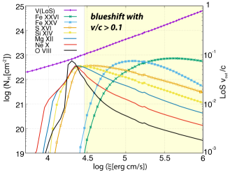
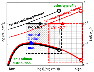
Figure 1: Left: An example of calculated AMD for multi-ion UFOs with MHD winds assuming $\Gamma=2,\theta=40^{\circ},p=1.2,f_{D}=1,\alpha_{\rm OX}=1.5$ and $\lambda_{\rm ion}=0.05$. Local hydrogen-equivalent columns (expressed on left ordinate) are shown for major ions; Fe xxvi (green), Fe xxv (cyan), S xvi (orange), Si xiv (yellow), Mg xii (dark blue), Ne x (red) and O viii (dark) along with the LoS wind velocity $v_{\rm out}/c$ (purple; expressed on right ordinate). A majority of the column is highly blueshifted ($v_{\rm out}/c>0.1$ in light yellow region) for many ions. Right: Schematics of AMD with velocity profiles $v_{\rm out}(\xi)$ for different ionizing photons corresponding to the ionic column (dark for less ionizing photons and red for more ionizing photons). Filled blue circle denotes where a local column is maximally produced. Open circle corresponds to the column produced at the innermost wind layer where $\xi$ value is the highest in each case. Note that the wind under higher ionization (in red) produces lower column of near-relativistic blueshift ($v_{\rm out}/c>0.1$ in squared domain) yielding slower UFOs in comparison with the lower ionization case (in shaded domain).

Therefore, the final UFO spectrum (mhdwind) is uniquely calculated by a set of these model parameters ($\theta,p,f_{D},\Gamma,\alpha_{\rm OX},\lambda_{\rm ion}$) for a given wind morphology. The range of the primary model parameters is listed in Table 1.

3 Results

3.1 Synthetic Multi-Ion Broadband UFO Spectra

As stated above, we aim to globally model the multi-ion UFO. We thus need to compute the ionic column densities $N^{i}_{\rm ion}$ for various chemical elements, most notably H/He-like ions; e.g. O viii, Ne x, Mg xii, Si xiv, S xvi, Fe xxv/Fe xxvi, Co xxvii, Ni xxviii, among others. Having this in mind, we handle the radiative processes between the wind material and the ionizing radiation following the prescription in our previous work (e.g. Fukumura et al., 2010a, 2017, 2021, reference therein). The photo-absorption cross-section $\sigma^{i}_{\rm abs}$ for a given ion is then calculated with the Voigt profile (e.g. Mihalas, 1978; Kotani et al., 2000; Hanke et al., 2009) using the simulated wind kinematics (e.g. Fukumura et al., 2010a).

In this framework, the line width (or shape) is naturally determined as a result of the internal wind velocity gradient (or shear velocity) $v_{\rm sh}$ along a LoS from the MHD wind model, which is typically on the order of $\sim 10\%$ of the LoS velocity itself at a given distance. Hence, we obtain the velocity shear directly for the Voigt function rather than employing an arbitrary “turbulent motion” parameterization.

With these quantities being available, the synthetic multi-ion UFO spectrum (mhdwind) is calculated by computing the line optical depth $\tau^{i}(E)$ as a function of energy $E$ such that

$$\tau^{i}(E)\equiv\sigma^{i}_{\rm abs}(v_{\rm sh};E)N^{i}_{\rm ion}(E)\ .$$ (7)

Therefore, the predicted broadband spectrum $f_{\rm obs}(E)\propto\Pi_{i}e^{-\tau^{i}(E)}$ is a function of wind-related parameters ($\theta,p,f_{D}$) coupled to the other parameters associated with radiation field ($\Gamma,\alpha_{\rm OX},\lambda_{\rm ion}$). This is how we simulate theoretical UFO spectra (mhdwind) as we aim to investigate spectral signatures that could be attributed to the generic features of MHD disk-winds perhaps in terms of the wind kinematics and/or density distribution as described above.

To better illustrate the underlying physics responsible for characterizing broadband absorption spectra as a consequence of radiative transfer, we show an example of the simulated AMD in Figure 1 (left) for a series of primary ions; local hydrogen-equivalent columns (value expressed on left ordinate) for Fe xxvi (green), Fe xxv (cyan), S xvi (orange), Si xiv (yellow), Mg xii (dark blue), Ne x (red) and O viii (dark) along with the LoS wind velocity $v_{\rm out}/c$ (purple; value expressed on right ordinate) assuming a fiducial set of parameters; i.e. $\Gamma=2,\theta=40^{\circ},p=1.2,f_{D}=1,\alpha_{\rm OX}=1.5$ and $\lambda_{\rm ion}=0.05$. While the exact AMD profile can vary from one case to the other depending on the input SED and wind conditions, this is one of the typically obtained ionic distributions relevant for Seyfert AGN UFOs in our calculations. It should be noted that the velocity profile $v_{\rm out}(\xi)$ is always unique in the sense that the fastest part of the wind at the innermost layer always possesses the highest ionization parameter value. This is because acceleration mechanism in our MHD framework is not due to radiation, but to magnetic processes (by both magnetocentrifugal and pressure gradient forces; e.g. Blandford & Payne 1982; Contopoulos & Lovelace 1994; Fukumura et al. 2010a). It is seen that the columns $N^{i}_{\rm ion}$ of individual ions are progressively produced over a large extent of LoS distance (or ionization parameter) as coronal X-ray radiation traverses the wind. The predominant fraction of the LoS-integrated column per ion is found in the higher ionization regime (i.e. in the vicinity of the central engine where the wind velocity is near-relativistic, $v/c\mathrel{\raise 2.15277pt\hbox{$>$}\mkern-14.0mu\lower 2.58334pt\hbox{$\sim$}}0.1$, in the light yellow region of the figure) responsible for the final absorption features we observe. The shape of a typical column profile is asymmetric in a way that the column rapidly falls off with decreasing $\xi$ (i.e. increasing distance) past its peak point where the maximum local column is produced; i.e. approximately at $\log\xi\sim 4.3$ for the soft X-ray absorbers while at $\log\xi\sim 5.0-5.5$ for Fe xxv/Fe xxvi ions. This AMD hence indicates that most of the ions (i.e. low-ionization ions such as O viii and high-ionization ions such as Fe xxvi) are necessarily near-relativistic (i.e. highly blueshifted) with an appreciable total column being identified as multi-ion UFOs, especially, Fe xxv/Fe xxvi being broader and faster.

Figure 1 (right) schematically depicts how the absorber’s velocity would change for different ionizing X-ray photons with respect to AMD. The velocity of the wind $v_{\rm out}$ at a given $\xi$ value is lower with more ionizing photons (red) compared to that with less ionizing photons (dark) because the velocity profile $v_{\rm out}(\xi)$ systematically shifts towards higher ionization with increasing ionizing luminosity as the innermost wind is always ionized the most. Given that the value of the ionic column is essentially determined by the ionization threshold, the production of local ionic column for a given element (e.g. Fe xxvi) occurs roughly in the same ionization range (solid dark/red curves). Filled blue circle denotes where the local column is maximally produced. The innermost wind irradiated by more (less) ionizing photons are labeled by red (dark) open circle where $\xi$ is the highest, as expected. In the presence of more ionizing photons in the illuminating SED (in red), the ionization parameter becomes higher by definition and the wind produces lower columns of near-relativistic blueshift (indicated by squared domain). As a consequence, the integrated column to be observed predominantly consists of those with lower blueshift, thus “slower” UFOs. In contrast, much of the total column is highly blueshifted if the ionizing photons in SED are less (in shaded domain), thus “faster” UFOs. Therefore, the differences in blueshift and ionic column due to the amount of ionizing photons inevitably lead to different absorption features as shall presented below in §3.1.1.

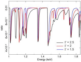
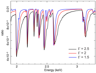
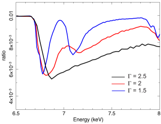
Figure 2: Theoretical multi-ion absorption spectra (ratio to the continuum) for different photon index $\Gamma$ with $\theta=30^{\circ},p=1.3,f_{D}=1,\alpha_{\rm OX}=1.5$ and $\lambda_{\rm ion}=0.1$.

3.1.1 Model Dependencies of Multi-Ion MHD Disk-Winds

To further follow up the significance of the simulated AMD shown in Figure 1, we calculate a number of multi-ion UFO spectra (mhdwind) by allowing for one parameter to be varied at a time. For example, the dependence of a power-law slope $\Gamma$ is shown in Figure 2 where we assume $\theta=30^{\circ},p=1.3,f_{D}=1,\alpha_{\rm OX}=1.5$ and $\lambda_{\rm ion}=0.1$. It is clear that the overall UFO signatures tend to be enhanced with softer (steeper) power-law component in the absence of efficient ionizing photons. Note that the trough energy in each absorption line remains almost unchanged, while the line width is dramatically affected as a result of ionization equilibrium because the corresponding velocity profile $v_{\rm out}(\xi)$ with AMD is accordingly shifted when $\Gamma$ changes, as depicted in Figure 1 (Right). When the SED is harder (i.e. smaller $\Gamma$), the inner layer (i.e. faster moving part) of the global MHD wind can be fully ionized producing little observable columns. Thus, the main absorption feature of the UFOs in that case will be governed predominantly by moderate or slower layer of the wind where the broadening is weakened but the centroid energy remains the same. This trend is systematically found in the broadband energy ranging from $\sim 1$ keV to Fe K complex. In particular, Fe xxv/Fe xxvi lines become so broad that the two are blended together for softer SED (e.g. $\Gamma=2.5$) as if it were a single edge feature.

In Figures 10-13 in Appendix A, we show more synthetic multi-ion absorption spectra of the mhdwind model to demonstrate various dependences on the model parameters. All in all, it is striking, and a common feature, that the most of the absorption features from different ions in these calculations are noticeably asymmetric such that blue tails are more extended and skewed towards higher energy. This is a manifestation of the unique AMD coupled to the MHD wind kinematics shown in Figure 1 as discussed in §3.1. That is, those columns produced from the wind at near-relativistic blueshift ($v/c\mathrel{\raise 2.15277pt\hbox{$>$}\mkern-14.0mu\lower 2.58334pt\hbox{$\sim$}}0.1$) largely dictate the asymmetric character in the spectrum as a “tell-tale” signature.

As mentioned earlier, one of the common spectral features from multi-ion UFOs in these calculations is blueshifted tails due to the generic kinematics of MHD-driven winds; i.e. the closer in to AGN, the faster the outflow. This unique characteristics of the magnetized wind can imprint a distinct absorption line profile through the shape of AMD as a consequence of photoionization balance as illustrated in Figure 3 (Left) (see also Figure 1). In comparison with other disk-wind models, the expected shape of the line profile from MHD-driven winds (red) is generally unique and distinctive enough to be separately identified. For example, line-driving (cyan) in general tends to produce an asymmetric line shape of an extended red wing (which is reversed to MHD-driving discussed here) due to an asymptotically increasing terminal wind velocity, whereas thermal-driving (green) allows for a relatively narrow line shape of little asymmetry because of a generically constant (slow) motion (C. Done and J. Reeves, in private communications). In contrast, a phenomenological Gaussian/Voigt line profiles (dashed) are symmetric.

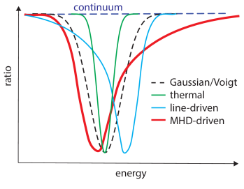
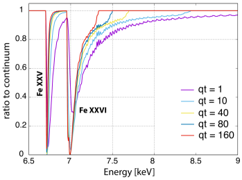
Figure 3: Left: Schematic diagram showing a comparison of characteristic absorption profiles among various wind driving mechanisms; Gaussian/Voigt profiles (dashed), thermal-driving (green), line-driving (cyan) and MHD-driving (red). Right: Spectral change in Fe xxv/Fe xxvi lines due to disk truncation at the inner launching radius parameterized by $q_{T}$.

On the other hand, it should be pointed out that the exact asymmetric line shape is very sensitive to the shape of AMD (including the velocity profile $v(\xi)$); the asymmetry could be minimized or even reversed depending on the underlying SED, wind property and other physical factors. Therefore, we emphasize that the obtained asymmetric line profiles here should be regarded as the most probable case on average.

Since we are focused on UFOs in the context of MHD driving, ionic columns are necessarily produced at smaller distances from AGN where the velocity is near-relativistic (see Fig. 1 (left)). Since the broadening of lines is determined by the wind shear velocity (from the LoS velocity gradient) at a given distance as discussed in §3.1, the line width tends to be very large considering that $v_{\rm shear}/v_{\rm out}\sim 0.1$ along a LoS. For this reason, the UFO spectra in our model tend to be broad such that subtle atomic line features might be blurred. For example, despite our expectation, no doublet structure is resolved for Fe xxvi Ly$\alpha$ lines (6.973 keV and 6.952 keV) due to blending, while it should be indeed identified in BH XRB disk winds because of their much lower velocities (e.g. Miller et al., 2015; Fukumura et al., 2021).

3.2 The Effects of the Inner Disk Truncation

Accretion disk winds in AGNs are often discussed in comparison with ionized outflows in BH XRBs. As an ideal laboratory owing to their much shorter time scale, sequenced X-ray observations of BH transient events can provide a valuable insight into wind’s morphology, variable nature and likely correlations, for example. Among those BH XRBs, a handful of systems are known to exhibit wind signatures in X-ray spectra. While there is no clear analogy for AGNs, pronounced disk winds are indeed present in BH XRBs during high/soft (bright) state, while winds appear to be extremely weak (if not absent) during low/hard (quiescent) state, as they go through a series of distinct accretion modes in the hardness-intensity diagram (aka. q-diagram) (e.g. Fender & Belloni, 2004; Fender et al., 2004; Remillard & McClintock, 2006; McClintock & Remillard, 2006; Done et al., 2007; Belloni, 2010; Ponti et al., 2012). During high/soft state, the standard thin accretion disks (Shakura & Sunyaev, 1973; Novikov & Thorne, 1973) in the context of general relativity are thought to extend all the way down to the ISCO based on X-ray observations of the thermal disk continuum (e.g. McClintock et al., 2014; Li et al., 2005; Shafee et al., 2006) and interpretations of asymmetric broad Fe line profiles (e.g. Fabian et al., 2000). On the other hand, it has been suggested that the inner disk may actually be truncated beyond the ISCO during low/hard state (as mass accretion rate drops), considering that the inner part of accretion becomes optically thin, hotter and radiatively inefficient (such as ADAF/ADIOS; e.g. Narayan & Yi 1994; Blandford & Begelman 1999) forming a compact corona around a BH that is surrounded by the standard thermal disk (e.g. Esin et al., 1997; Done et al., 2007). While such a speculation has gained much attention, the disk truncation signatures, also independently derived from reflection spectroscopy and reverberation lags, have still remained elusive observationally (e.g. Shidatsu et al., 2011; Petrucci et al., 2014; Plant et al., 2015; García et al., 2015; De Marco et al., 2017).

To follow up a possibility of inner disk truncation in the context of Seyfert UFOs, we consider here a possible consequence of such a truncation of the inner disk. Given that the MHD-driven UFOs are primarily launched from the innermost region of the disk (where the Keplerian motion is fast and ionization state is high; see Figure 1), it is expected that removing the inner part of the disk should significantly reduce the amount of near-relativistic plasma (i.e. UFOs) to be launched. As a result, the observed UFO line profile could be substantially less blueshifted depending on the truncation radius $R_{T}$. To probe this effect, we take one of our template runs (i.e. $\theta=40^{\circ},\Gamma=2,\alpha_{OX}=1.5$…) and calculate a line spectrum by parameterizing $R_{T}$ as $R_{T}\equiv q_{T}R_{\rm in}\sim q_{T}R_{\rm ISCO}$ where we set $q_{T}=1,10,40,80$ and $160$. That is, the disk is not truncated for $q_{T}=1$, while extremely truncated at large distance for $q_{T}=160$. Figure 3 (Right) demonstrates the effect of $q_{T}$ on Fe xxv/Fe xxvi lines as an example. It is seen that the most blueshifted part of the feature is gradually disappearing with increasing $q_{T}$ as expected, whereas the centroid absorption structure (with small blueshift) remains almost unaffected as it is produced by the exterior wind that is launched from the outer part of the disk. Note that the line depth is almost independent of $q_{T}$ since it is predominantly determined by the wind density factor $f_{D}$ which is fixed in this work.

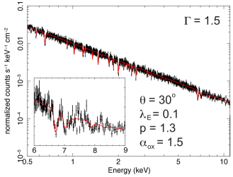
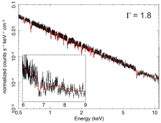
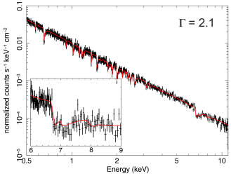
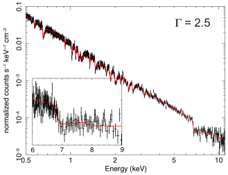
Figure 4: Simulated 100ks XRISM/Resolve spectra for different photon index $\Gamma$ with $\theta=30^{\circ},p=1.3,\alpha_{\rm OX}=1.5,f_{D}=1$ and $\lambda_{\rm ion}=0.1$. Inset shows a close-up of Fe K absorbers.

3.3 The Effects of Soft Excess

Given that a good fraction of Seyfert 1 AGNs exhibits soft X-ray excess (SE), another unique soft X-ray component, in their SED (i.e. more than 50% to 90%; e.g. Turner & Pounds 1989; Crummy et al. 2006; Boissay et al. 2016), we also consider a possible effect of SE on the UFO signatures. Although SE is present in the energy band lower than the most of the major UFO lines (e.g. Mg xii, Si xiv, S xvi and Fe K ions), a potential impact of radiative transfer on the production of these UFO columns is yet to be known. For an illustration purpose, we use a single blackbody of temperature $kT_{\rm SE}=100$ eV to phenomenologically mimic the SE component in SED, which is usually a reasonable representation of it. For simplicity, it is assumed here that SE originates almost entirely from the same region producing the primary emission or completely within the launching region of the outflows; i.e. no “diffuse” (larger than flow cone base) component of the SE. We then make a comparison, with and without SE in an assumed SED, by performing radiative transfer calculations with XSTAR to see the resulting UFO spectra.

Figure 5 Left shows a representative comparison of calculated AMD for selected ions with SE (solid; its normalization of $K_{\rm SE}=3\times 10^{-8}$) and without SE (dashed) in the injected SED of $\Gamma=2$ and $\alpha_{\rm OX}=1.5$ with the rest of the model parameters being the same in both cases. It is seen that the ionization front for various transitions are almost systematically shifted towards higher $\xi$ regime (corresponding spatially to smaller distances to the BH) due to the extra soft photons from the SE, allowing the produced UFOs to be more blueshifted and broader in the spectrum. There is little change, though, in the calculated column.

To confirm this view, we further calculate a broadband UFO spectrum based on a similar set of parameters by assuming different SE normalizations in Figure 5 Right; $K_{\rm SE}=3\times 10^{-8}$ (moderate in blue) and $6\times 10^{-7}$ (strong in red) cases. As demonstrated, the presence of SE could have a significant impact on the broadband multi-ion UFO spectra depending on its strength. In an extreme case of a strong SE flux, a large fraction of ionic column per transition line can be produced in the inner faster regions of the MHD wind in a way that the resulting absorption lines may be broad enough to be blended together (e.g. in red) in theory purely due to radiative transfer process (i.e. photoionization). Given that the presence of SE tends to make ionizing spectrum softer, it is consistent that the physical role of SE in UFO spectral features is qualitatively very similar to that by softer X-ray slope as shown in Figure 2 in §3.1.1.

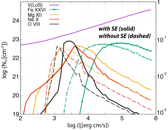
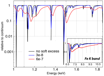
Figure 5: Left: Sample comparison of AMD, similar to Figure 1, with (solid) and without (dashed) SE flux in the injected SED for selected ions assuming $\theta=40^{\circ},p=1.3,\alpha_{\rm OX}=1.5,f_{D}=1$ and $\lambda_{\rm ion}=0.05$. Right: Theoretical multi-ion absorption spectra (ratio to the continuum) for different SE normalization of $K_{\rm SE}=6\times 10^{-7}$ (strong in red) and $3\times 10^{-8}$ (moderate in blue) in comparison with the absence of SE (in dark) assuming $\theta=30^{\circ},p=1.3,\alpha_{\rm OX}=1.5,f_{D}=0.1$ and $\lambda_{\rm ion}=0.05$.

3.4 Spectral Simulations with Microcalorimeters

By exploiting a library of theoretical spectra of multi-ion UFOs presented in §3.1, we further investigate observational implications here in an anticipation of upcoming microcalorimeter missions with XRISM/Resolve and Athena/X-IFU in an effort to realistically assess a plausibility of constraining the UFO signatures. For subsequent simulations, we use xarm_res_h5ev_20170818.rmf for XRISM and XIFU_CC_BASELINECONF_2018_10_10_EXTENDED_LSF.rmf for Athena through this work.

3.4.1 Feasibility with XRISM/Resolve Observations

Assuming a fiducial 2-10 keV X-ray flux of $\sim 2.3\times 10^{-11}$ erg cm^-2 s^-1 for canonical Seyfert AGNs, we perform spectral simulations of the models considered in §3.1 with 100ks XRISM/Resolve exposure. These are idealized simulations considering only the theoretical UFO component with no additional spectral complexity.

Figure 4 shows the simulated spectra for different $\Gamma$ where the richness of the UFO features seem to be well captured ranging from $\sim 0.5$ keV to the Fe K complex band. The overall asymmetry of multi-ion absorbers are still traceable in these simulated data to the extent that the expected “tell-tale” MHD-driving signature can be resolved especially for softer X-ray spectrum where the wind is less overionized when a fewer number of hard X-ray photons can participate in ionization. The other simulated XRISM/Resolve spectra for various dependences are also shown in Figure 14-17 in Appendix B.

3.4.2 Convolution of UFOs with Additional Absorbers in Simulated Data

Observed X-ray spectra of a large number of radio-quiet Seyfert AGNs are generally well known to contain multiple absorption components including broadband complex atomic features; e.g. warm absorbers, typically characterized by a series of ions at different charge states (e.g. Crenshaw, Kraemer & George, 2003; Blustin et al., 2005; Steenbrugge et al., 2005; McKernan et al., 2007; Holczer et al., 2007; Detmers et al., 2011; Fukumura et al., 2018; Laha et al., 2021). Due to the atomic physics, primarily dictated by the oscillator strength and Einstein coefficient for individual resonant transitions per ion, stronger warm absorbers on average are predominantly given by H/He-like species appearing in the soft X-ray to UV band (also occasionally accompanied by Fe L-shell transitions and unresolved transition array (UTA) due to 2p-3d transitions in Fe M-shell ions as well; e.g. Behar et al. 2001a, b; Netzer 2004). In addition, some Seyfert AGN spectra occasionally give a hint at the presence of partially covering ionized materials (e.g. Matzeu et al., 2016).

To make a more realistic diagnosis for a plausible detection of MHD-driven UFO features by robustly constraining the wind parameters, we simulate another microcalorimater spectrum based on a similar set of MHD UFO model that are now convolved with these additional absorption components. That is, we adopt a template spectral model, mhdwind mtable model, of $\Gamma=2,\alpha_{\rm OX}=1.5,\theta=35^{\circ},p=1.25,f_{D}=0.1,$ and $\lambda_{\rm ion}=0.08$, as a test case. For warm absorbers, we follow the conventional approach by employing a three-zone warmabs model generated with xstar2xspec such that

$${\tt warmabs}=\left\{\begin{array}[]{llr}N_{H}=10^{21},\log\xi=2,v_{\rm out}/c=0.001&~{}~{}\textmd{(cold gas)},\\ N_{H}=10^{22},\log\xi=3,v_{\rm out}/c=0.003&~{}~{}\textmd{(warm gas)},\\ N_{H}=10^{23},\log\xi=4,v_{\rm out}/c=0.01&~{}~{}\textmd{(hot gas)},\end{array}\right.$$ (11)

assuming a power-law continuum of $\Gamma=2$ and a uniform turbulent velocity of $\sigma=500$ km s^-1 (e.g. Kaspi et al., 2000; Netzer et al., 2003; Krongold et al., 2003; Blustin et al., 2005; Gabel et al., 2005). Independently, a partially covering ionized absorber (perhaps in a discrete patchy cloud) is represented with zxipcf model Miller et al. (2006); Reeves et al. (2008) by

$${\tt zxipcf}=\left\{\begin{array}[]{llr}N_{H}=5\times 10^{23},\log\xi=4,v_{\rm out}/c=0.01&~{}~{}\textmd{(partial absorbers)},\\ \end{array}\right.$$ (13)

with a turbulent velocity of 200 km s^-1 and the covering fraction of 0.5. Thus, the composite model is expressed symbolically as

$${\tt composite=tbabs\times po\times mhdwind\times warmabs_{\tt C}\times warmabs_{\tt W}\times warmabs_{\tt H}\times zxipcf}$$ (14)

where the subscript denotes each warm absorber zone in equation (11), which is combined with the partial covering absorber (zxipcf) in equation (13) while being multiplied by the underlying power-law spectrum (po) and the Galactic neutral absorber (tbabs) with $N_{H}^{\rm Gal}=10^{20}$ cm^-2. We then generate a 100ks XRISM/Resolve spectrum assuming the same 2-10 keV flux of $\sim 2.3\times 10^{-11}$ erg cm^-2 s^-1 as is considered in §3.2.1.

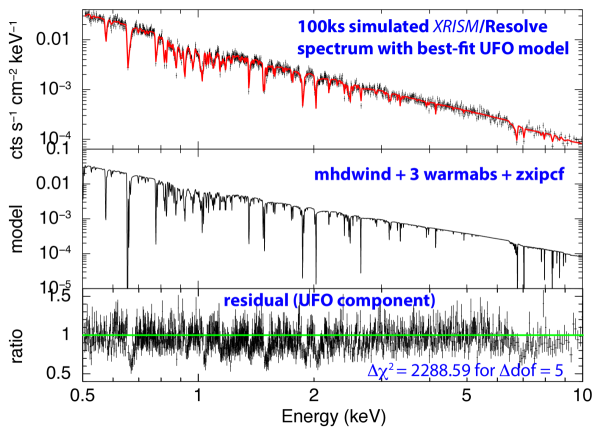
Figure 6: Upper: Simulated 100ks XRISM/Resolve spectrum (in dark) for $\theta=35^{\circ},p=1.25,\Gamma=2,\alpha_{\rm OX}=1.5,f_{D}=0.1$ and $\lambda_{\rm ion}=0.08$ with the best-fit composite model (in red). See Table 2 for the best-fit model parameters. Middle: Unfolded best-fit model spectrum. Lower: Residuals in the form of data/model ratio in the absence of the UFO component (mhdwind).

Table 2: Best-Fit Composite Model for 100 ks Simulated XRISM/Resolve Spectrum

Component	Parameter	Best-Fit Value	Model Value
tbabs	$N_{H}^{\rm Gal}$ [cm-2]	$10^{20}$†	$10^{20}$†
po	$\Gamma$	$2.00^{+0.01}_{-0.01}$	2
mhdwind	$\alpha_{\rm OX}$	$1.51^{+0.02}_{\rm-1.51}$	1.5
	$\lambda_{\rm ion}$	$0.081_{-0.004}^{+0.003}$	0.08
	$\theta$ [deg]	$34.9_{-1.0}^{+2.1}$	35
	$p$	$1.22_{-1.22}^{+0.04}$	1.25
	$f_{D}$	$0.074_{-0.01}^{+0.03}$	0.1
warmabs	$N_{\rm H,Cold}$	$1.01_{-1.01}^{+0.33}\times 10^{21}$	$10^{21}$
	$\log\xi_{\rm Cold}$	$1.95_{-0.07}^{+0.08}$	$2$
	$v_{\rm out,Cold}/c$	$-8.74_{-4.5}^{+3.3}\times 10^{-4}$	$10^{-3}$
	$N_{\rm H,Warm}$	$1.00_{-0.06}^{+0.29}\times 10^{22}$	$10^{22}$
	$\log\xi_{\rm Warm}$	$2.97_{-0.02}^{+0.03}$	$3$
	$v_{\rm out,Warm}/c$	$-2.96_{-0.14}^{+0.12}\times 10^{-3}$	$3\times 10^{-3}$
	$N_{\rm H,Hot}$	$1.1_{-0.16}^{+0.59}\times 10^{22}$	$10^{22}$
	$\log\xi_{\rm Hot}$	$4.00_{-0.04}^{+0.04}$	$4$
	$v_{\rm out,Hot}/c$	$-9.80_{-0.23}^{+0.24}\times 10^{-3}$	$10^{-2}$
zxipcf	$N_{\rm H,zxipcf}$	$4.00_{-1.09}^{+1.35}\times 10^{23}$	$5\times 10^{23}$
	$\log\xi_{\rm zxipcf}$	$3.98_{-0.08}^{+0.07}$	$4$
	$v_{\rm out,zxipcf}/c$	$-1.00_{-0.01}^{+0.01}\times 10^{-2}$	$10^{-2}$
	$\chi^{2}/$dof	$15930.27/18982$   (18218.86/18987)‡

We assume $M=10^{8}M_{\odot}$, $f_{\rm 2-10keV}=2.3\times 10^{-11}$ erg cm^-2 s^-1 and $L_{\rm ion}=10^{44}$ erg s^-1.
^† Fixed.    ^‡ In the absence of the UFO component (mhdwind).

The simulated XRISM/Resolve spectrum is first generated based on the composite wind model expressed in equation (8). We then fit the mock data with the same model to retrieve the best-fit broadband spectrum of multi-ion UFOs by allowing mhdwind, warmabs and zxipcf componets to be varied simultaneously (except for the fixed turbulence velocities). The upper panel of Figure 6 shows the simulated spectrum (in dark) along with the folded best-fit model (in red). The middle panel shows the unfolded best-fit model. A number of UFO signatures in this simulated spectrum seems to be well accounted for by the composite model successfully constraining the UFO parameters at a reasonable statistical significance (yielding $\chi^{2}$/dof=15930.27/18982). The best-fit parameters for the simulated spectrum are listed in Table 2. When fitted with the composite wind model, the broadband UFO features are unambiguously resolved and the correct parameter values are successfully retained within a reasonably narrow range of uncertainties. It is seen that the predicted UFO signatures of relatively broad line profiles of asymmetry appear to be immune to the spectral contamination by external absorbers under this particular parameter set. The uniquely blueshifted UFO line shape of asymmetry (discussed in §3 and Figure 3) is still unmistakenly preserved and identified by simple visual inspection.

To see the significance of mhdwind component in the spectrum, we subsequently removed the UFO component (mhdwind) from the best-fit spectrum (composite). The lower panel of Figure 6 now shows the residuals (in the form of data/model ratio) after the subtraction of the UFO component (mhdwind) to examine whether the “tell-tale” sign of the UFO signatures can still be observed in data. We find that the unique spectral features of MHD-driven UFOs of multiple ions in mhdwind are clearly seen in the residual, thus enabling mhdwind component to be successfully disentangled. Without mhdwind component, the best-fit model becomes significantly worse resulting in $\chi^{2}$/dof=18218.86/18987 (i.e. $\Delta\chi^{2}=2288.59$ for $\Delta$dof = 5 by removing four mhdwind parameters). Therefore, this simulation potentially demonstrates a realistic viability of extracting MHD-driven UFO signatures of multiple ions in the presence of contaminating non-UFO absorbers.

From a technical perspective, it is known that bright Seyfert AGN spectra often exhibit reflection components resulting from photons reprocessed by disks (e.g. Magdziarz & Zdziarski, 1995; Ross & Fabian, 2005). It is hence conceivable that such reflection (consisting of a series of atomic features such as emission and absorption/edges as well as Compton hump) might also contaminate the underlying UFO signatures. We further investigate the impact of such reflection features by implementing both xillverCp (for distant reflection) and relxillCp (for relativistic reflection) models (García et al., 2013) in XRISM/Resolve simulations. In Appendix C we present a 100 ks XRISM/Resolve spectrum with a fiducial reflection component to find that even in that case the expected MHD spectral signatures indeed remain preserved.

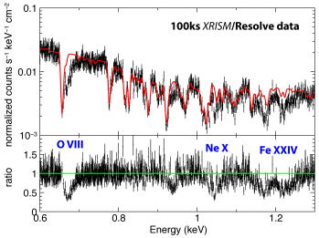
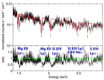
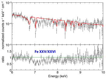
Figure 7: Zoom-in on simulated 100 ks XRISM/Resolve spectrum for $\Gamma=2,\alpha_{\rm OX}=1.5,\lambda_{\rm ion}=0.08,p=1.3,f_{D}=0.1$ and $\theta=35^{\circ}$ showing the residual (ratio) from the best-fit composite model (composite in red) in the absence of MHD UFO component (mhdwind).

We further look into ion-by-ion UFO components in a simulated broadband spectrum in order to support our claim that microcalorimeter data can in fact be exploited as a powerful diagnostic tool to realistically identify MHD-driving montages such as unique asymmetric line profiles (see Fig. 3 left). In Figure 7 we are focused on a series of major absorption lines from a 100 ks XRISM/Resolve simulation for $\Gamma=2,\alpha_{\rm OX}=1.5,\lambda_{\rm ion}=0.08,p=1.3,f_{D}=0.1$ and $\theta=35^{\circ}$ showing the residual (ratio) from the best-fit composite model (composite in red) in the absence of MHD UFO component (mhdwind). As demonstrated earlier, a clear UFO signature of asymmetric (broad) line is undoubtedly seen for this multi-ion MHD UFO whose shape is not necessarily matched with the phenomenological Gaussian or Voigt functions. While the exact shape and strength (i.e. line optical depth and equivalent width) of each line depends sensitively on wind parameters, the characteristic UFO features are systematically imprinted in the broadband.

In anticipating for the next generation X-ray microcalorimeter instrument beyond XRISM mission, we also explore an observational viability of our MHD UFO model by performing a number of simulations with Athena/X-IFU instrument. Assuming an almost identical set of fiducial model parameters as considered for XRISM simulations, broadband UFO spectra of multi-ion are simulated with 10 ks Athena/X-IFU exposure assuming $\Gamma=2,\alpha_{\rm OX}=1.5,\lambda_{\rm ion}=0.1,p=1.2$ and $\theta=35^{\circ}$ in Figure 8 in comparison with the earlier XRISM/Resolve simulations in Figure 7. It is obvious that the same simulated UFO features are further refined at more statistically significant level even with 10 ks exposure, owing to Athena’s large collecting area. In this simplified comparison, it is thus implied in principle that more than ten time-resolved observations could be made with Athena to obtain data of the same spectroscopic quality expected from a single 100 ks XRISM observation in an attempt to ambitiously conduct an outflow reverberation mapping for (highly) variable nature of the observed UFOs (e.g. Matzeu et al., 2016; Parker et al., 2018).

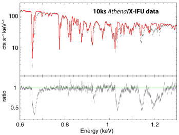
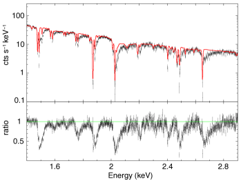
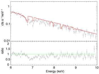
Figure 8: Zoom-in on simulated 10 ks Athena/X-IFU spectrum for $\Gamma=2,\alpha_{\rm OX}=1.5,\lambda_{\rm ion}=0.1,p=1.2,f_{D}=0.1$ and $\theta=35^{\circ}$ showing the residual (ratio) from the best-fit composite model (composite in red) in the absence of MHD UFO component (mhdwind).

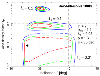
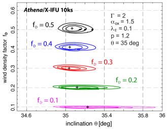
Figure 9: Confidence contours of $(\theta,f_{D})$ for different values of wind density factor $f_{D}$ derived from the best-fit models with $\theta=35^{\circ}$ showing 68% (red), 90% (green) and 99% (blue) levels. Left: XRISM/Resolve 100 ks exposure. Right: Athena/X-IFU 10 ks exposure.

Finally, we compare the statistical confidence in constraining, for example, the inclination $\theta$, for different wind density factor $f_{D}$ in Figure 9 (left) where their best-fit values are shown for low ($f_{D}=0.01$), intermediate ($f_{D}=0.1$) and high ($f_{D}=0.5$) density values assuming $p=1.3,\theta=35^{\circ}$ and $\lambda_{\rm ion}=0.05$ for the simulated 100ks XRISM/Resolve data. The expected uncertainties in both quantities are relatively small enabling one to robustly retain the correct UFO parameters with 100 ks XRISM/Resolve exposure unless the wind density (i.e. $f_{D}$) is too low. This is because the predicted absorption lines would become very narrow and weak due to the inner part of the wind being almost fully ionized (where the wind is near-relativistic) if $f_{D}$ is very low. Again, a mere 10 ks exposure with Athena/X-IFU is found to drastically improve such a limitation to constraining the UFO parameters even for very weak UFO features (i.e. low $f_{D}$) as shown in Figure 9 (right), demonstrating a high efficacy in accurately recovering the correct values of $f_{D}$ as well as inclination $\theta$, as an example.

4 Summary & Discussion

In this work, we conduct a systematic spectral modeling of the multi-ion X-ray UFO features (i.e. $\sim 0.5-10$ keV range) relevant for radio-quiet Seyfert AGNs in the context of MHD-driven accretion disk winds. Considering some generic features of MHD-driven UFOs, our primary focus is to investigate whether or not there exist some unique spectral signatures mainly attributed to MHD driving in predicted UFO absorption lines that can be seen in observations. By exploiting a set of six parameters in our MHD wind model, namely, X-ray photon index ($\Gamma$), X-ray to O/UV strength ($\alpha_{\rm OX}$), ionizing luminosity ratio ($\lambda_{\rm ion}$), inclination angle ($\theta$), wind density factor ($f_{D}$) and wind density slope ($p$), we have shown on average that many of the synthetic UFO spectra commonly exhibit an asymmetric line profile of an extended blue tail toward higher energy manifesting the underlying MHD wind kinematics through photoionization. As demonstrated by the AMD in Figure 1, our MHD-wind model allows for simultaneous multi-ion UFOs (i.e. ranging from low to high ionization absorbers such as O viii and Fe xxvi) in the broadband X-ray spectrum. All the calculations assume the solar abundances throughout this work (i.e. $A_{\rm ion}=A_{\rm ion,\odot}$).

We further perform a series of microcalorimeter simulations based on the synthetic UFO spectra in the broadband (mhdwind) in anticipation of the future X-ray missions with XRISM/Resolve and Athena/X-IFU instruments to better examine an observational viability of the model. Assuming a set of fiducial parameters, we find that the unique asymmetric signature of blueshift in multi-ion UFO lines can be well captured in many simulated spectra. To realistically test its plausibility of detection, additional absorption components are independently added to our simulations in the form of 3-zone warm absorbers composed of cold, warm and hot plasma (warmabs) as well as a partially covering ionized gas (zxipcf). Despite the presence of such a spectral contamination, it is demonstrated that the predicted UFO signatures in mhdwind are unambiguously retained in the simulated data. If indeed imprinted in high fidelity microcalorimeter spectra, it is conceivable that the predicted UFO lines of unique features can be potentially used as a diagnostic proxy to differentiate different launching mechanisms proposed today.

In the present formalism, a number of complications are not taken into account for simplicity. First, we treat the primary parameters ($\theta,p,f_{D},\Gamma,\alpha_{\rm OX},\lambda_{\rm ion}$) being independent of each other (see Fig. 4 and other dependences in Appendices). In reality, it has been reported, for instance, that some observable AGN measurements appear to be (tightly) correlated in various samples of AGN surveys; e.g. $\Gamma$, $\alpha_{\rm OX}$, Eddington ratio and monochromatic UV luminosities (e.g. Steffen et al., 2006; Shemmer et al., 2008; Luo et al., 2014; Laurenti et al., 2021). Although these correlations are preferentially suggested in highly-accreting quasars, this may well be relevant for Seyfert 1s accreting at low Eddington rate. If this is the case, our simulation results could be less relevant in certain parameter space that we have probed in this work; e.g. X-ray bright AGNs at high Eddington ratio (i.e. higher $\lambda_{\rm ion}$ with smaller $|\alpha_{\rm OX}|$ and/or higher $\lambda_{\rm ion}$ with softer $\Gamma$). This would need to be considered for quantitative simulations specific to individual AGN/quasar UFOs.

Additional complications associated to spectral features include SE and reflection components often seen in many Seyfert AGNs. We phenomenologically add SE component in our fiducial AGN SED to calculate its effect and find a significant role in changing ionization structure of the wind through radiative transfer such that almost all major ions of various charge state tend to be produced at smaller distances (towards the BH) in higher ionization state where the MHD wind is faster. Stronger SE causes multi-ion UFO lines to be more blueshifted and broader in a way similar to the role of photon index $\Gamma$, both of which involves more soft photons being available for photoionization. On the other hand, the presence of reflection features (i.e. emission and absorption/edges) is also considered as another source of spectral contamination against the expected MHD-driven UFO signatures. By implementing xillver and relxill models, we perform a similar 100ks microcalorimeter simulation for XRISM/Resolve. It is demonstrated that even a relatively pronounced reflection flux (e.g. refl_frac=2 and $A_{\rm Fe}/A_{\rm Fe,\odot}=5$) does not significantly distort the tell-tale MHD signature of the blueshifted UFO absorbers.

We emphasize that our choice of defining the Eddington ratio, $\lambda_{\rm ion}$, is simply a convenient way to control the X-ray luminosity $L_{\rm ion}$ responsible for photoionization in this model (see §2.2). More subtle factors related to $L_{\rm ion}$ (e.g. radiative efficiency in accretion power, black hole spin, coronal geometry and disk structure) have been ignored to avoid further complications and extra degrees of freedom in this problem. It is also expected that X-ray luminosity should be intimately tied to wind density (i.e. $n_{o}$ in our model) determined by the disk density that essentially signifies accretion rate. In our calculations, a fixed value of the wind density factor $f_{D}$ is naively decoupled from our Eddington ratio $\lambda_{\rm ion}$. As addressed earlier, the mass accretion rate (thus the wind density normalization parameterized by $f_{D}$) should in reality be physically coupled to the X-ray luminosity and perhaps $\alpha_{\rm OX}$, for example, as suggested in the past studies (e.g. Steffen et al., 2006; Shemmer et al., 2008; Luo et al., 2014; Laurenti et al., 2021). For this reason, it is not our primary interest to compare the absolute line properties (i.e. line optical depth and EW), which is subject to the value of $f_{D}$. Instead, our main focus is the relative comparison of line shape of multi-ion UFOs from one case to the other so one can learn a systematic trend as a whole rather than a specific quantitative change. Another prescription of X-ray luminosity such as $L_{\rm ion}\propto f_{D}$, for example, would hence be more physically motivated as is often employed in our past spectral analyses (e.g. Fukumura et al., 2017, 2018, 2021), which, however, is beyond the scope of the present work.

Our microcalorimeter simulations clearly show a high efficacy of retaining the expected multi-ion UFO components in the composite broadband spectrum for a given set of model parameters, indicating a persistent immunity of the UFO features against the external contaminations due to other forms of ionized absorbers. This immunity, however, is not always warranted depending on a number of conditions. We simply assume a typical 2-10 keV flux of $\sim 2.3\times 10^{-11}$ erg cm^-2 s^-1 with certain exposures as a test case for Seyfert 1 AGNs, but disentangling the predicted MHD-driven UFO features (i.e. near-relativistic blueshift of asymmetry to higher energy) could obviously become more challenging and very enigmatic in some cases (e.g. lower flux and shorter exposure). Therefore, given the model limitation due to the fixed value of $f_{D}$ in our simulations, the absolute values of the model parameters that set the appearance and disappearance of multi-ion UFOs (shown in our calculated spectra) should not be regarded as the generalized values, although a qualitative trend can still be learned from those calculations.

With the photon statistics achievable with the current spectroscopic instruments, it is not easy to conduct time-resolved analysis of rapid UFO variability. As demonstrated in Figure 9 for a given UFO parameter set, only a 10 ks exposure with Athena/X-IFU appears to be sufficient to robustly resolve these Seyfert UFOs owing to its large collecting area. This would revolutionize the physics of UFOs since it can enable us to take a series of snapshot spectra, each of which on a much shorter timescale that is currently possible. By being able to study a temporal response of individual UFO absorbers ranging from soft X-ray band to Fe K lines, spectroscopic information can be further cast into timing property of various absorbing ions, from which one could potentially make a geometrical (spatial) diagnosis of multiple ions in the UFOs as the continuum varies in time. This is another reason why multi-ion UFO modeling, and not just Fe K absorbers, is important for understanding a global picture of the UFOs. Such a reverberation mapping of multi-ion UFOs has been partially hinted at with the use of principal component analysis (PCA) of XMM-Newton/EPIC data in order to study in detail the correlations between the continuum source and the multiple ions in the observed UFOs (e.g. Parker et al., 2018).

Concerning the expected asymmetric line profiles unique to MHD-driving process, there have been some observational hints of the expected asymmetric Fe K UFO features in NuSTAR and XMM-Newton data (e.g. a nearby Seyfert 2 AGN, MCG-03-58-007 in Braito et al. 2022; a lensed broad absorption line quasar, APM 08279+5255 in Chartas et al. 2009; a complex Fe K trough feature seen in narrow-line Seyfert, 1H 0707-495 in Hagino et al. 2017, among others). Also, it might be relevant for other types of disk-winds such as those of BH XRBs occasionally detected, for example, with Chandra, in Galactic transients (e.g. Miller et al., 2015; Chakraborty et al., 2021) as well as AGN warm absorbers (e.g. Kaspi et al., 2000; Kallman et al., 2009; Fukumura et al., 2017). The observed velocities of the ionized outflows in these systems are much lower than those in UFOs; i.e. a few hundred to at most a thousand km s^-1. The expected blueshift is thus only up to $v/c\mathrel{\raise 1.29167pt\hbox{$<$}\mkern-14.0mu\lower 2.58334pt\hbox{$\sim$}}0.01$ meaning that the line width is at most $\Delta E/E\mathrel{\raise 1.29167pt\hbox{$<$}\mkern-14.0mu\lower 2.58334pt\hbox{$\sim$}}0.001$. This implies that the characteristic asymmetry would be observationally more intangible even if indeed magnetically launched in those systems. While it might still be plausible to differentiate between MHD-driving (with such an asymmetry of smaller magnitude) and, for example, another promising process such as thermal-driving (C. Done, in private communications), a robust disentanglement could be perhaps less trivial while not impossible. Again, analyzing multiple ions rather than a single Fe K feature would be a great complement in order to probe a wide range of ionization structure in the wind.

In this work, we do not incorporate emission lines also expected to originate from the same outflowing gas or separate regions. For example, Monte Carlo approach has been often employed to calculate self-consistent emission and scattering components (e.g. Hagino et al. 2015, 2016, 2017 with MONACO and Sim et al. 2008, 2010a, 2010b also including special relativistic effects), while XCORT has utilized XSTAR runs (Schurch & Done, 2007). More recently, Luminari et al. (2018) has proposed WINE model with a special focus on detailed special relativistic dimming for UFOs (see also Luminari et al., 2020, 2021). Such emission process might be important to accurately assess the physical properties of ionized absorbers because they can “fill in” the intrinsic absorption features. For example, some very luminous quasars accreting at near-Eddington rate such as PDS 456 is found to show a broad P-Cygni profile in Fe K band associated with its prototype UFO where the wind may well be Compton-thick (Nardini et al., 2015). On the other hand, one of the well-studied Seyfert 1 AGN showing canonical X-ray warm absorbers, NGC 3783, is also known to exhibit a handful emission lines in UV/soft X-ray band mostly from the He-like triplets (resonance, intercombination, and forbidden lines) of O vii, Ne ix, and Mg xi as well as Ly$\alpha$ lines from the H-like species of these elements with a very small systematic velocity shift ($130\pm 290$ km s^-1; Kaspi et al. 2000, e.g.; Gabel et al. 2005, e.g.; Kallman et al. 2009, e.g.). However, given a moderate accretion rate in Seyfert 1 population with typically very weak (if not none) P-Cygni profiles in X-ray spectra, it is reasonable to speculate that X-ray absorbing gas is most likely optically thin. Scattering within the absorbers might then be less efficient.

While we further investigate in this paper a possible effect of inner disk truncation on UFO spectra (see §3.2), a slight change in UFO kinematics and/or wind density could also naturally change UFO line profiles without invoking a geometric change in disk configuration (i.e. truncation). Hence, such a degeneracy may make it physically challenging to uniquely attribute variable nature of UFOs to only disk truncation in observations especially in AGNs where phenomenology of accretion flows still remains very enigmatic (e.g. Antonucci, 2013). It is also hard to identify “state transition” of accretion mode due to their much longer time scales. On the other hand, we have similarly considered a potential impact of disk truncation in the context of AGN warm absorbers and BH XRB disk-winds in the past (Fukumura et al., 2021), and we would like to note, in the context of MHD scenario, that the inner disk truncation in those slow/moderate disk winds would not significantly change the absorption features in contrast with UFOs. This is because the ionized ions responsible for non-UFOs are produced in a part of the wind that is predominantly launched from much larger disk radii from the BH, thus the inner truncation would play little role in reshaping the absorption lines. The inner disk truncation therefore results in a distinct consequence in absorption spectra between UFOs and non-UFOs.

Considering the elusive origin of the UFO and its launching mechanism, this work is originally motivated by the notion that a detailed UFO spectral feature may potentially shed light on the underlying physics of UFOs. As one of the promising scenarios, we exploit the MHD-driving process by calculating synthetic UFO spectra of multiple ions in the broadband X-ray. As illustrated in Figure 3 (left), the predicted UFO line shape is generally found to be uniquely asymmetric with an extended blue tail attributed to the generic kinematics of MHD disk-winds; i.e. the closer in to the BH, the faster the wind. While this is indeed a generic spectral signature in most of the calculations made so far, such a claim should be understood with care. That is, it is conceivable that the degree of such characteristic asymmetric signature may be made very small to the extent that the expected asymmetry could become virtually unnoticeable in observations depending on the wind condition and or AGN properties. This point is intimately related to AMD and velocity distribution addressed in §3.1 (see Figure 1). On the other hand, another leading scenario, line-driving process tends to imprint a different tell-tale sign in the UFO line shape that is generally reversed to MHD-driven UFO spectra because of its different underlying wind kinematics; i.e. the gas accelerates along a LoS by radiation pressure until it asymptotically reaches a finite terminal velocity (thus coasting) at large distance (e.g. Shlosman & Vitello, 1993; Kniggle et al., 1995; Long & Kniggle, 2002; Sim et al., 2008; Hagino et al., 2015). Such a distinct velocity field of line-driven UFOs is generally expected to produce a broad asymmetric UFO line spectrum with an extended red tail being fundamentally distinct from that by MHD-winds (e.g. Long & Kniggle, 2002; Sim, 2005; Sim et al., 2010a, b; Hagino et al., 2015; Mizumoto et al., 2021, also Reeves J. N. in private communication). Nonetheless, it is possible again that the apparent difference between two models could be made either too small or too subtle in some specific cases to observationally enable us to robustly differentiate. Hence, we emphasize that our claim for obtaining the unique spectral features due to MHD-driving should be viewed as an average feature. With this caution in mind, we believe that our modeling and simulations in this work can help improve our fundamental understanding of the physics of X-ray UFOs that could otherwise be observationally inaccessible.

Appendix A: Model Dependences of Synthetic Multi-Ion Broadband UFO Spectra

As part of investigating the model parameter dependences, we explore the effect of X-ray hardness via $\Gamma$ on the UFO line profiles in §3.1. In the Appendix A, the effects of the other model parameters (see Table 1) are considered and demonstrated. We examine the dependence of X-ray strength relative to optical/UV flux parameterized by $\alpha_{\rm OX}$ in Figure 10 with $\theta=30^{\circ},\Gamma=2,p=1.3,f_{D}=1$ and $\lambda_{\rm ion}=0.1$. Although the selected range of $\alpha_{\rm OX}$ in this work is limited, we clearly see its strong effect on the UFO spectra. By suppressing more X-ray photons relative to UV photons (i.e. larger $|\alpha_{\rm OX}|$ value), for example, the resulting velocity curve $v(\xi)$ tends to shift towards lower $\xi$ domain with AMD (see Figure 1b) producing more blueshifted UFO lines with larger width. As similarly seen in Figure 2, soft X-ray UFO features are more sensitive to the change in X-ray strength compared to Fe K UFOs. Trough energies in individual lines are more noticeably blueshifted with increasing $|\alpha_{\rm OX}|$, while there is little change due to $\Gamma$ in Figure 2.

The effect of ionizing luminosity in units of Eddington luminosity $\lambda_{\rm ion}$ is explored in Figure 11 with $\theta=30^{\circ},\Gamma=2,p=1.3,f_{D}=1$ and $\alpha_{\rm OX}=1.5$. In a simplified situation where only ionizing luminosity is varied while being decoupled from spectral shape (i.e. $\Gamma$ and $\alpha_{\rm OX}$), we find that the UFO signatures are weakened in general with increasing $\lambda_{\rm ion}$ as naturally expected. In comparison, the spectral dependence is less sensitive to $\lambda_{\rm ion}$ than it is to spectral indices, especially for soft X-ray UFOs. Understanding of this trend, however, needs some caution because the variation of X-ray luminosity in AGNs is often accompanied by the change in spectral shape as well, which is not currently taken into account in these calculations for simplicity. We shall discuss more on this point later in §4.

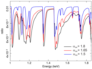
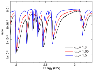
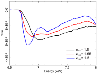
Figure 10: Theoretical multi-ion absorption spectra (ratio to the continuum) for different X-ray strength $\alpha_{\rm OX}$ with $\theta=30^{\circ},\Gamma=2,p=1.3,f_{D}=1$ and $\lambda_{\rm ion}=0.1$.

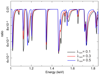
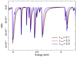
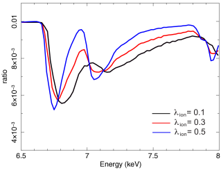
Figure 11: Theoretical multi-ion absorption spectra (ratio to the continuum) for different ionizing luminosity ratio $\lambda_{\rm ion}$ with $\theta=30^{\circ},\Gamma=2,p=1.3,f_{D}=1$ and $\alpha_{\rm OX}=1.5$.

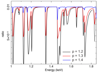
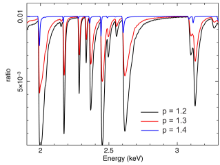
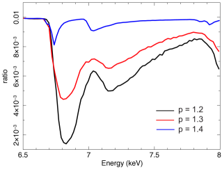
Figure 12: Theoretical multi-ion absorption spectra (ratio to the continuum) for different density slope $p$ with $\theta=30^{\circ},\Gamma=2,\alpha_{\rm OX}=1.5,f_{D}=1$ and $\lambda_{\rm ion}=0.1$.

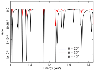
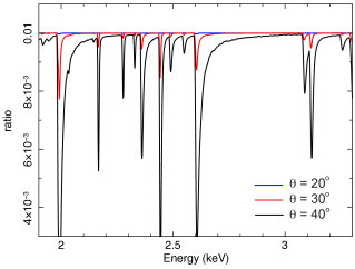
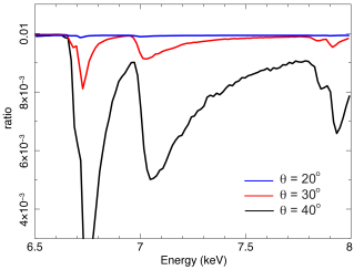
Figure 13: Theoretical multi-ion absorption spectra (ratio to the continuum) for different inclination $\theta$ with $\Gamma=2,\alpha_{\rm OX}=1.5,p=1.3,f_{D}=1$ and $\lambda_{\rm ion}=0.1$.

In addition to the effect of photoionization due to differences in the radiation field, we further study the dependence on the wind conditions. In Figure 12 we show the UFO spectra for various wind density gradients with $p$ assuming $\theta=30^{\circ},\Gamma=2,\alpha_{\rm OX}=1.5,f_{D}=1$ and $\lambda_{\rm ion}=0.1$. In this exercise, soft X-ray UFOs (located at larger distances from AGN) have lower density with increasing $p$, whereas Fe K UFOs are impacted the least, as the innermost wind at the launching radius remains fixed (at $r\sim R_{\rm in}=6R_{g}$). As a result, soft X-ray UFO signatures in the spectrum are significantly weakened, for example, for $p=1.4$, as expected. With $p=1.2$ wind density structure, on the other hand, the broadband UFO features are clearly present being attributed to an almost equal column $N^{i}_{\rm ion}$ for all ions as expected from AMD (see §2.2).

Finally, we consider spectral dependence on inclination $\theta$ in Figure 13 assuming $\Gamma=2,\alpha_{\rm OX}=1.5,p=1.3,f_{D}=1$ and $\lambda_{\rm ion}=0.1$. The obtained dependence is two-fold; i.e. a combination of velocity change and wind density variation with $\theta$. This is because the LoS wind velocity (i.e. velocity component projected onto LoS direction) is dependent on the relative angle between the LoS orientation and a tangential direction of magnetic field lines. At the same time, the wind density is lower by many orders of magnitude near the funnel region close to the symmetry axis (e.g. Blandford & Payne, 1982; Contopoulos & Lovelace, 1994; Fukumura et al., 2014; Chakravorty et al., 2016). These factors combined together generally cause the absorption lines to be dramatically weaker and less blueshifted with decreasing $\theta$.

Appendix B: Model Dependences of Simulated Multi-Ion Broadband UFO Spectra

To further follow up the XRISM/Resolve simulations of our MHD UFO models discussed in §3.3.1, we present here in Figures 14-17 the other simulated spectra for various model parameters listed in Table 1.

In Figure 14, the well-defined blueshifted UFO features of asymmetry is similarly seen in which X-ray-weak AGNs (e.g. $\alpha_{\rm OX}=1.8$) can clearly imprint such an asymmetric blueshift structure in the spectrum, most notably seen in Fe K lines. Note that Fe xxv and Fe xxvi lines are made so broad that they are blended together to form a single feature, for example, for $\Gamma=2.5$ and $\alpha_{\rm OX}=1.8$. As expected from the synthetic spectra in Figure 11, simulated data for different ionizing luminosity $\lambda_{\rm ion}$ in Figure 15 do not seem to change much with $\lambda_{\rm ion}$, while the suppression of atomic lines, especially in the soft X-ray band, are found. Since the wind density slope and inclination can probably provide the most direct effect on the absorption spectra, dramatic changes in UFO signatures are indeed coded in XRISM/Resolve data as demonstrated in Figures 16 and 17. For example, it is found that microcalorimeters are capable of detecting a series of blueshifted lines of unique asymmetry in the soft X-ray UFOs as well as a pronounced Fe K UFOs for $p=1.2$ winds. For a fixed wind density factor $f_{D}=1$, the simulated spectrum would exhibit little wind features for $p=1.5-1.7$, as is previously shown from the model with $p=1.4$ in Figure 12. Similarly, very weak line features expected from a polar wind with $\theta=20^{\circ}$ would not be visible even with 80ks microcalorimeter observation under this parameter set, as indicated earlier in Figure 13. On the other hand, low inclination winds of $\theta=30^{\circ}-40^{\circ}$, being relevant for canonical Seyfert 1 AGNs, would be securely resolved. Moderate inclination winds of $\theta=50^{\circ}$ would prominently exhibit stronger UFO features.

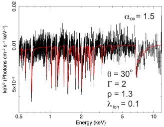
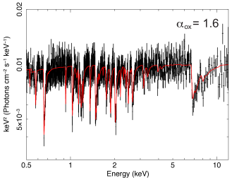
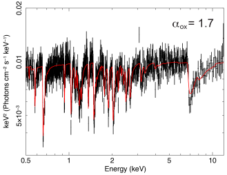
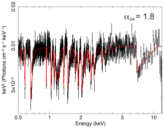
Figure 14: Simulated 100ks XRISM/Resolve spectra for different X-ray strength $\alpha_{\rm OX}$ with $\theta=30^{\circ},p=1.3,f_{D}=1,\Gamma=2$ and $\lambda_{\rm ion}=0.1$.

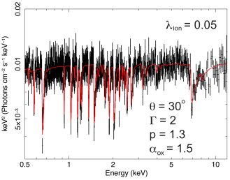
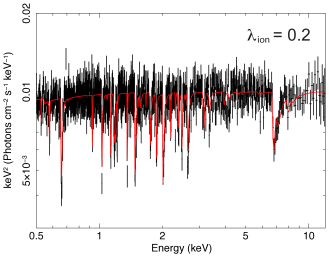
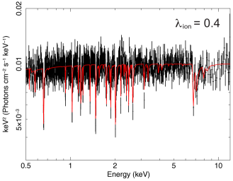
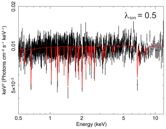
Figure 15: Simulated 100ks XRISM/Resolve spectra for different ionizing luminosity ratio $\lambda_{\rm ion}$ with $\theta=30^{\circ},p=1.3,f_{D}=1,\Gamma=2$ and $\alpha_{\rm OX}=1.5$.

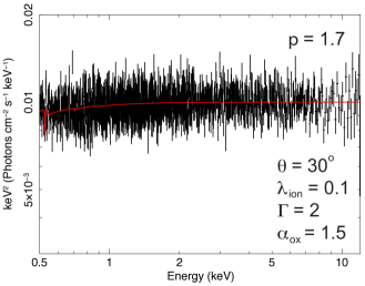
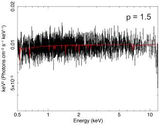
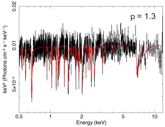
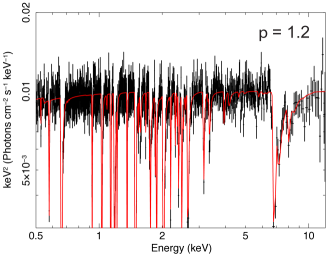
Figure 16: Simulated 100ks XRISM/Resolve spectra for different density slope $p$ with $\theta=30^{\circ},\Gamma=2,\alpha_{\rm OX}=1.5,f_{D}=1$ and $\lambda_{\rm ion}=0.1$.

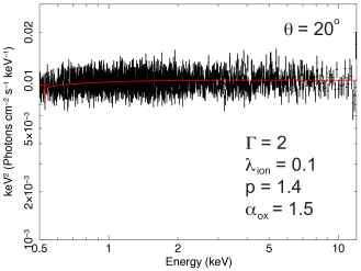
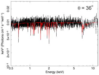
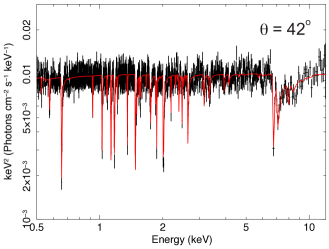
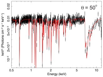
Figure 17: Simulated 100ks XRISM/Resolve spectra for different inclination $\theta$ with $\Gamma=2,p=1.4,\alpha_{\rm OX}=1.5,f_{D}=1$ and $\lambda_{\rm ion}=0.1$.

Appendix C: Impact of Reflection Component on Simulated Multi-Ion Broadband UFO Spectra

One of the characteristic spectral features often identified in bright Seyfert AGNs is reflection features from disks; i.e. Compton hump and various atomic lines including emission and absorption/edges due to reprocessed photons (e.g. Magdziarz & Zdziarski, 1995; Ross & Fabian, 2005). To follow up our investigations on a persistent presence of MHD signatures in UFO spectra, we further examine the effects of such reflection component and see if the expected characteristics of asymmetric line profiles might be contaminated or distorted to the extent that identification of the MHD-driven UFO features may be difficult as a consequence.

To this end, we replace a single power-law (po) by adding both xillverCp (for distant reflection) and relxillCp (for relativistic reflection) models in the original composite model (as shown in Table 2 and Fig. 6) for XRISM/Resolve simulations; i.e. a new composite model is expressed symbolically as

$${\tt tbabs\times(relxillCp+xillverCp)\times mhdwind\times warmabs_{\tt C}\times warmabs_{\tt W}\times warmabs_{\tt H}\times zxipcf}$$ (15)

where we have fixed a number of baseline parameter values in the reflection components to minimize the extra degrees of freedom, while others are to be varied to find the bestfit solution. Figure 18 demonstrates a feasibility of extracting the MHD signatures of the expected UFO spectrum lines in such a case. We set the normalizations of the reflection components such that the 2-10 keV flux remains of the order of $10^{-11}$ erg cm^-2 s^-1 as considered earlier in §3.3.2 where reflection feature is absent. In this simulation, we assume a relatively strong reflection contribution to the underlying continuum; e.g. refl_frac = 2 and $A_{\rm Fe}/A_{\rm Fe,\odot}=5$. In order to reduce the extra degrees of freedom in the model, we fix the emissivity profile of the disk emission in such a way that $\epsilon(r)\propto r^{-6}$ for $r/R_{g}\leq 10$ (the innermost) and $\propto r^{-3}$ for $r/R_{g}>10$ (the outer part) to take into account relativistic effects under strong gravity (these parameters are thus frozen throughout fitting) for the dimensionless BH spin of $a=0.98$. The assumed parameter values and the bestfit model parameters are listed in Table 3.

It is clearly demonstrated that the spectral signatures of UFOs due to the MHD wind component are still unambiguously imprinted in the broadband spectrum (i.e. extended asymmetric blue tails) despite the complex spectral curvature of relatively strong reflection flux including the extra absorption lines. Identification of the individual MHD-driven UFO lines in the bestfit model is equally robust as that in the power-law continuum simulation (in the absence of reflection; see Fig. 6) indicating that the reflection features interfere very little with the UFO lines to the extent that the predicted tell-tale MHD signatures are less likely to be washed out. The adopted parameter values of MHD wind component (mhdwind) are almost all well retained by fitting the simulated spectra in both cases (see Tables 2 and 3). Note that even strong Fe K emission lines (both narrow and broad) in this simulation does not significantly distort the original Fe K UFO absorption feature.

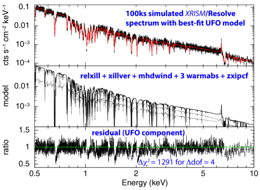
Figure 18: Similar to Figure 6 but in the presence of reflection component.

Table 3: Best-Fit Composite Model for 100 ks Simulated XRISM/Resolve Spectrum with Reflection

Component	Parameter	Best-Fit Value	Model Value
tbabs	$N_{H}^{\rm Gal}$ [cm-2]	$10^{20}$†	$10^{20}$†
xillverCp	$\Gamma$	$2.01^{+0.01}_{-0.01}$	2 ♭
	$\theta$ [deg]	$36.8_{-1.9}^{+2.5}$	$35$ ♭
	AFe [AFe,⊙]	$5.04_{-0.61}^{+0.98}$	5 ♭
	$kT_{e}$ [keV]	$163$ △	150 ♭
	refl_frac	$1.82_{-0.37}^{+0.44}$	2 ♭
	$\log n_{D}\rm{[cm^{-3}]}$	$18.9_{-0.11}^{+0.08}$	19 ♭
	$\log\xi$	$0.96_{-0.09}^{+0.09}$	1
	Kref [$10^{-4}$]	$0.73_{-0.11}^{+0.17}$	1 ♭
relxillCp♯	$a/M$	$0.979_{-0.013}^{+0.010}$	0.98
	$\log\xi$	$2.96_{-0.10}^{+0.09}$	3
mhdwind	$\alpha_{\rm OX}$	$1.50^{+0.01}_{p}$	1.5
	$\Gamma$	$2.01^{+0.01}_{-0.01}$	2 ♭
	$\lambda_{\rm ion}$	$0.084_{-0.003}^{+0.003}$	0.08
	$\theta$ [deg]	$36.8_{-1.9}^{+2.5}$	$35$ ♭
	$p$	$1.26_{-0.03}^{+0.03}$	1.25
	$f_{D}$	$0.093_{-0.01}^{+0.02}$	0.1
warmabs	$N_{\rm H,Cold}$	$1.01_{-1.01}^{+0.33}\times 10^{21}$	$10^{21}$
	$\log\xi_{\rm Cold}$	$2.05_{-0.05}^{+0.05}$	$2$
	$v_{\rm out,Cold}/c$	$-8.74_{-4.5}^{+3.3}\times 10^{-4}$	$10^{-3}$
	$N_{\rm H,Warm}$	$1.00_{-0.06}^{+0.29}\times 10^{22}$	$10^{22}$
	$\log\xi_{\rm Warm}$	$2.97_{-0.02}^{+0.03}$	$3$
	$v_{\rm out,Warm}/c$	$-2.96_{-0.14}^{+0.12}\times 10^{-3}$	$3\times 10^{-3}$
	$N_{\rm H,Hot}$	$1.0_{-0.02}^{p}\times 10^{23}$	$10^{23}$
	$\log\xi_{\rm Hot}$	$4.00_{-0.01}^{+0.01}$	$4$
	$v_{\rm out,Hot}/c$	$-1.0_{-0.07}^{+0.08}\times 10^{-2}$	$10^{-2}$
zxipcf	$N_{\rm H,zxipcf}$	$4.05_{-0.9}^{+1.0}\times 10^{23}$	$5\times 10^{23}$
	$\log\xi_{\rm zxipcf}$	$3.95_{-0.07}^{+0.06}$	$4$
	$v_{\rm out,zxipcf}/c$	$-1.00_{-0.09}^{+0.01}\times 10^{-2}$	$10^{-2}$
	$\chi^{2}/$dof	$19681.51/18975$   (20972.51/18979)‡

^♯ Disk emissivity law is fixed as $\epsilon\propto r^{-6}$ and $r^{-3}$ across $R_{\rm break}/R_{g}=10$ in relxill.
^△ Unconstrained. ^♭ Tied among models.    ^‡ In the absence of the UFO component (mhdwind).
^p Pegged values.

References

- Antonucci (2013) Antonucci, R. 2013, Nature, 495, 165
- Arav et al. (2015) Arav, N. et al. 2015, A&A, 577, 37
- Bardeen et al. (1972) Bardeen, J. M., Press, W. H. & Teukolsky, S. A. 1972, ApJ, 178, 347
- Barret et al. (2018) Barret, D. et al. 2018, SPIE, 10699
- Behar (2009) Behar, E., 2009, ApJ, 703, 1346
- Behar et al. (2001b) Behar, E., Sako, M. & Kahn, S. M. 2001b, ApJ, 563, 497
- Behar et al. (2001a) Behar, E., Cottam, J. & Kahn, S. M. 2001a, ApJ, 548, 966
- Belloni (2010) Belloni, T. M. 2010, The Jet Paradigm, Lecture Notes in Physics, 794, p.53
- Blandford & Payne (1982) Blandford, R. D. & Payne, D. G. 1982, MNRAS, 199, 883
- Blandford & Begelman (1999) Blandford, R. R & Begelman, M. C. 1999, MNRAS, 303, L1
- Blustin et al. (2005) Blustin, A. J., Page, M. J., Fuerst, S. V., Branduardi-Raymont, G. & Ashton, C. E. 2005, A&A, 431, 111
- Boissay et al. (2016) Boissay, R. Ricci, C. & Paltani, S. 2016, A&A, 588, A70
- Boissay-Malaquin et al. (2019) Boissay-Malaquin, R., Danehkar, A., Marshall, H. L. & Nowak, M. A. 2019, ApJ, 873, 29
- Braito et al. (2022) Braito, V., Reeves, J. N., Matzeu, G., Severgnini, P., Ballo, L., Cicone, C., Ceca, R. D., Giustini, M. & Sirressi, M. 2022, ApJ, 926, 219
- Chakraborty et al. (2021) Chakraborty, S., Ratheesh, A., Bhattacharyya, S., Tomsick, J. A., Tombesi, F., Fukumura, K. & Jaisawal, G. K. 2021, MNRAS, 508, 475
- Chakravorty et al. (2016) Chakravorty, S., Petrucci, P.-O., Ferreira, J., Henri, G., Belmont, R., Clavel, M., Corbel, S., Rodriguez, J., Coriat, M., Drappeau, S. & Malzac, J. 2016, A&A, 589, 119
- Chartas et al. (2009) Chartas, G., Saez, C., Brandt, W. N., Giustini, M., & Garmire, G. P. 2009, ApJ, 706, 644
- Chartas & Canas (2018) Chartas, G. & Canas, M. H. 2018, ApJ, 867, 103
- Chartas et al. (2021) Chartas, G., Cappi, M., Vignali, C., Dadina, M., James, V., Lanzuisi, G., Giustini, M., Gaspari, M., Strickland, S. & Bertola, E. 2021, ApJ, 920, 24
- Contopoulos & Lovelace (1994) Contopoulos, J. & Lovelace, R. V. E. 1994, ApJ, 429, 139
- Crenshaw, Kraemer & George (2003) Crenshaw, D. M., Kraemer, S.B. & George, I. M. 2003 Annu. Rev. Astron. & Astrophys. 2003, 41, 117
- Crummy et al. (2006) Crummy, J., Fabian, A. C., Gallo, L. & Ross, R. R. 2006, MNRAS, 365, 1067
- Cunningham (1975) Cunningham, C. T. 1975, ApJ, 202, 788
- De Marco et al. (2017) De Marco, B. et al. 2017, MNRAS, 471, 1475
- Detmers et al. (2011) Detmers, R. G. et al. 2011, A&A, 534, 38
- Done et al. (2007) Done, C., Gierlinski, M. & Kubota, A. 2007, A&ARv, 15, 1
- Esin et al. (1997) Esin, A. A., McClintock, J. E., & Narayan, R. 1997, ApJ, 489, 865
- Everett (2005) Everett, J. E. 2005, ApJ, 631, 689
- Fabian et al. (2000) Fabian, A. C., Iwasawa, K., Reynolds, C. S. & Young, A. J. 2000, PASP, 112, 1145
- Faucher-Giguère & Quataert (2012) Faucher-Giguère, C.-A., Quataert, E. 2012, MNRAS, 425, 605
- Fender et al. (2004) Fender, R. P., Belloni, T. M. & Gallo, E. 2004, MNRAS, 355, 1105
- Fender & Belloni (2004) Fender, R. & Belloni, T. 2004, ARAA, 42, 317
- Ferreira (1997) Ferreira, J. 1997, A&A, 319, 340
- Fukumura et al. (2010a) Fukumura, K., Kazanas, D., Contopoulos, I. & Behar, E. 2010a, ApJ, 715, 636
- Fukumura et al. (2010b) Fukumura, K., Kazanas, D., Contopoulos, I. & Behar, E. 2010b, ApJ, 723, L228
- Fukumura et al. (2014) Fukumura, K., Tombesi, F., Kazanas, D., Shrader, C., Behar, E. & Contopoulos, I. 2014, ApJ, 780, 120
- Fukumura et al. (2015) Fukumura, K., Tombesi, F., Kazanas, D., Shrader, C., Behar, E. & Contopoulos, I. 2015, ApJ, 805, 17
- Fukumura et al. (2017) Fukumura, K., Kazanas, D., Shrader, C., D., Behar, E., Tombesi, F. & Contopoulos, I. 2017, Nature Astronomy, 1, 0062
- Fukumura et al. (2018) Fukumura, K., Kazanas, D., Shrader, C., Behar, E., Tombesi, F. & Contopoulos, I. 2018, ApJ, 853, 40
- Fukumura et al. (2021) Fukumura, K., Kazanas, D., Shrader, C., Tombesi, F., Kalapotharakos, C. & Behar, E. 2021, ApJ, 912, 86
- García et al. (2013) García, J. A., Dauser, T. , Reynolds, C. S., Kallman, T. R., McClintock, J. E., Wilms, J. & Eikmann, W. 2013, ApJ, 768, 146
- García et al. (2015) García, J. A., Steiner, J. F., McClintock, J. E., Remillard, R. A., Grinberg, V. Dauser, T. 2015, ApJ, 813, 84
- Gabel et al. (2005) Gabel, J. R. et al. 2005, ApJ, 631, 741
- Gofford et al. (2015) Gofford, J., Reeves, J. N., McLaughlin, D. E., Braito, V., Turner, T. J., Tombesi, F. & Cappi, M. 2015, MNRAS, 451, 4169
- Giustini & Proga (2012) Giustini, M. & Proga, D. 2012, ApJ, 758, 70
- Gupta et al. (2013) Gupta, A., Mathur, S., Krongold, Y. & Nicastro, F. 2013, ApJ, 772, 66
- Gupta et al. (2015) Gupta, A., Mathur, S. & Krongold, Y. 2015, ApJ, 798, 4
- Hagino et al. (2015) Hagino, K., Odaka, H., Done, C., Gandhi, P., Watanabe, S., Sako, M. & Takahashi, T. 2015, MNRAS, 446, 663
- Hagino et al. (2016) Hagino, K., Odaka, H., Done, C., Tomaru, R., Watanabe, S. & Takahashi, T. 2016, MNRAS, 461, 3954
- Hagino et al. (2017) Hagino, K., Done, C., Odaka, H., Watanabe, S. & Takahashi, T. 2017, MNRAS, 468, 1442
- Hamann et al. (2018) Hamann, F., Chartas, G., Reeves, J. & Nardini, E. 2018, MNRAS, 476, 943
- Hanke et al. (2009) Hanke, M., Wilms, J., Nowak, M. A., Pottschmidt, K., Schulz, N. S. & Lee, J. C. 2009, ApJ, 690, 330
- Higginbottom et al. (2014) Higginbottom, N., Proga, D., Knigge, C., Long, K. S., Matthews, J. H. & Sim, S. A. 2014, ApJ, 789, 19
- Holczer et al. (2007) Holczer, T., Behar, E. & Kaspi, S. 2007, ApJ, 663, 799
- Holczer et al. (2010) Holczer, T., Behar, E. & Arav, N. 2010, ApJ, 708, 981 981
- Jacquemin-Ide et al. (2019) Jacquemin-Ide, J., Ferreira, J. & Lesur, G. 2019, MNRAS, 490, 3112
- Jacquemin-Ide et al. (2021) Jacquemin-Ide, J., Lesur, G. & Ferreira, J. 2021, A&A, 647, 192
- Kallman & Dorodnitsyn (2019) Kallman, T. & Dorodnitsyn, A. 2019, ApJ, 884, 111
- Kallman et al. (2009) Kallman, T. R., Bautista, M. A., Goriely, S., Mendoza, C., Miller, J. M., Palmeri, P., Quinet, P. & Raymond, J. 2009, ApJ, 701, 865
- Kallman & Bautista (2001) Kallman, T., & Bautista, M. 2001, ApJS, 133, 221
- Kaspi et al. (2000) Kaspi, S., Brandt, W. N., Netzer, H., Sambruna, R., Chartas, G., Garmire, G. P. & Nousek, J. A. 2000, ApJ, 535, 17
- Köngl & Kartje (1994) Köngl, A. & Kartje, J. F. 1994, ApJ, 434, 446
- Kotani et al. (2000) Kotani, T., Ebisawa, K., Dotani, T., Inoue, H., Nagase, F., Tanaka, Y. & Ueda, Y. 2000, ApJ, 539, 413
- Kazanas et al. (2012) Kazanas, D., Fukumura, K., Contopoulos, I., Behar, E. & Shrader, C. R. 2012, Astronomical Review, 7, 92
- Kazanas (2019) Kazanas, D. 2019, Galaxies, 7, 13
- Kallman & Bautista (2001) Kallman, T. & Bautista, M. 2001, ApJS, 133, 221
- Kniggle et al. (1995) Knigge, C., Woods, J. A. & Drew, J. E. 1995, MNRAS, 273, 225
- Krongold et al. (2003) Krongold, Y., Nicastro, F., Brickhouse, N. S., Elvis, M., Liedahl, D. A. & Mathur, S. 2003, ApJ, 597, 832
- Krongold et al. (2021) Krongold, Y., Longinotti, A. L., Santos-Lleó, M., Mathur, S., Peterson, B. M., Nicastro, F., Gupta, A., Rodríguez-Pascual, P. & Elías-Chávez, M. 2021, ApJ, 917, 39
- Kraemer et al. (2018) Kraemer, S. B., Tombesi, F. & Bottorff, M. C. 2018, ApJ, 852, 35
- Laha et al. (2021) Laha, S., Reynolds, C. S., Reeves, J., Kriss, G., Guainazzi, M., Smith, R., Veilleux, S. & Proga, D. 2021, Nature Astronomy, 5, 13
- Li et al. (2005) Li, L.-X., Zimmerman, E. R., Narayan, R. & McClintock, J. E. 2005, ApJS, 157, 335
- Laurenti et al. (2021) Laurenti, M. et al. 2021, accepted to A&A (arXiv:2110.06939)
- Long & Kniggle (2002) Long, K. S. & Knigge, C. 2002, ApJ, 579, 725
- Luminari et al. (2018) Luminari, A., Piconcelli, E., Tombesi, F., Zappacosta, L., Fiore, F., Piro, L. & Vagnetti, F. 2018, A&A, 619, 149
- Luminari et al. (2020) Luminari, A.,Tombesi, F., Piconcelli, E., Nicastro, F., Fukumura, K., Kazanas, D., Fiore, F. & Zappacosta, L. 2020, A&A,633, 55
- Luminari et al. (2021) Luminari, A., Nicastro, F., Elvis, M., Piconcelli, E., Tombesi, F., Zappacosta, L. & Fiore, F. 2021, A&A, 646, 111
- Luo et al. (2014) Luo, B. et al. 2014, 794, 70
- Magdziarz & Zdziarski (1995) Magdziarz, P. & Zdziarski, A. A. 1995, MNRAS, 273, 837
- McClintock et al. (2014) McClintock, J. E., Narayan, R. & Steiner, J. F. 2014, Space Science Reviews, 183, 295
- McClintock & Remillard (2006) McClintock, J. E. & Remillard, R. A. 2006 (arxiv:astro-ph/0306213)
- McKernan et al. (2007) McKernan, B., Yaqoob, T. & Reynolds, C. S. 2007, MNRAS, 379, 1359
- Marinucci et al. (2018) Marinucci, A., Bianchi, S., Braito, V., Matt, G., Nardini, E. & Reeves, J. 2018, MNRAS, 478, 5651
- Matzeu et al. (2016) Matzeu, G. A., Reeves, J. N., Nardini, E., Braito, V., Costa, M. T., Tombesi, F. & Gofford, J. 2016, MNRAS, 458, 1311
- Matzeu et al. (2017) Matzeu, G. A., Reeves, J. N., Braito, V., Nardini, E., McLaughlin, D. E., Lobban, A. P., Tombesi, F. & Costa, M. T. 2017, MNRAS, 472, 15
- Mihalas (1978) Mihalas, D. 1978, Stellar Atmospheres (2nd ed.; New York: W. H. Freeman & Company)
- Miller et al. (2006) Miller, L., Turner, T. J., Reeves, J. N., George, I. M., Porquet, D., Nandra, K. & Dovciak, M. 2006, A&A, 453, L13
- Miller et al. (2015) Miller, J. M., Fabian, A. C., Kaastra, J., Kallman, T., King, A. L., Proga, D., Raymond, J. & Reynolds, C. S. 2015, ApJ, 814, 87
- Nardini et al. (2015) Nardini, E. et al. 2015, Science, 347, 860
- Mizumoto et al. (2021) Mizumoto, M., Nomura, M. & Done, C. 2021, MNRAS, 503, 1442
- Narayan & Yi (1994) Narayan, R. & Yi, I. 1994, ApJ, 428, L13
- Netzer et al. (2003) Netzer, H. et al. 2003, ApJ, 599, 933
- Netzer (2004) Netzer, H. 2004, ApJ, 604, 551
- Nomura & Ohsuga (2017) Nomura, M. & Ohsuga, K. 2017, MNRAS, 465, 2873
- Novikov & Thorne (1973) Novikov, I. D. & Thorne, K. S. 1973, Black holes (Les astres occlus), p. 343-450. Edited by C. DeWitt and B. DeWitt, Gordon and Breach, N.Y.
- Parker et al. (2017) Parker, M. L. et al. 2017, Nature, 543, 83
- Parker et al. (2018) Parker, M. L., Reeves, J. N., Matzeu, G. A., Buisson, D. J. K. & Fabian, A. C. 2018, MNRAS, 474, 108 (Pa18)
- Pinto et al. (2018) Pinto, C., Alston, W., Parker, M. L., Fabian, A. C., Gallo, L. C., Buisson, D. J. K., Walton, D. J., Kara, E., Jiang, J., Lohfink, A. & Reynolds, C. S. 2018, MNRAS, 476, 1021
- Ponti et al. (2012) Ponti, G. et al. 2012, MNRAS, 422, L11
- Pounds et al. (2003) Pounds, K. A., Reeves, J. N., King, A. R., Page, K. L., O’Brien, P. T. & Turner, M. J. L. 2003, MNRAS, 345, 705
- Proga et al. (2000) Proga, D., Stone, J. M., & Kallman, T. R. 2000, ApJ, 543, 686
- Proga (2003) Proga, D. 2003, ApJ, 585, 406
- Ratheesh et al. (2021) Ratheesh, A., Tombesi, F., Fukumura, K., Soffitta, P., Costa, E. & Kazanas, D. 2021, A&A, 646, 154
- Reeves et al. (2003) Reeves, J. N., O’Brien, P. T. & Ward, M. J. 2003, ApJ, 593, 65
- Reeves et al. (2008) Reeves, J. N., Done, C., Pounds, K., Terashima, Y., Hayashida, K., Anabuki, N., Uchino, M. & Turner, M. 2008, MNRAS, 385, 108
- Reeves et al. (2009) Reeves, J. N., O’Brien, P. T., Braito, V., Behar, E., Miller, L., Turner, T. J., Fabian, A. C., Kaspi, S., Mushotzky, R. & Ward, M. 2009, ApJ, 701, 493
- Reeves et al. (2018a) Reeves, J. N., Braito, V., Nardini, E., Lobban, A. P., Matzeu, G. A. & Costa, M. T. 2018a, ApJ, 854, L8
- Reeves et al. (2018b) Reeves, J. N., Lobban, A. & Pounds, K. A. 2018b, ApJ, 854, 28
- Reeves et al. (2020) Reeves, J. N., Braito, V., Chartas, C., Hamann, F., Laha, S. & Nardini, E. 2020, ApJ, 895, 37
- Remillard & McClintock (2006) Remillard, R. A. & McClintock, J. E. 2006, ARA&A, 44, 49
- Reynolds (1997) Reynolds, C. S. 1997, MNRAS, 286, 513
- Risaliti & Elvis (2004) Risaliti, G. & Elvis, M. 2004, ASSL, 308, 187
- Ross & Fabian (2005) Ross, R. R. & Fabian, A. C. 2005, MNRAS, 358, 211
- Schurch & Done (2007) Schurch, N. J. & Done, C. 2007, MNRAS, 381, 1413
- Serafinelli et al. (2019) Serafinelli, R., Tombesi, F., Vagnetti, F., Piconcelli, E., Gaspari, M., & Saturni, F. G. 2019, A&A, 627, 121
- Shafee et al. (2006) Shafee, R., McClintock, J. E., Narayan, R., Davis, S. W., Li, Li-Xin & Remillard, R. A. 2006, ApJ, 636, 113
- Shakura & Sunyaev (1973) Shakura, N. I. & Sunyaev, R. A. 1973, A&A, 24, 337
- Plant et al. (2015) Plant, D. S., Fender, R. P., Ponti, G., Muñoz-Darias, T. & Coriat, M. 2015, A&A 573, 120
- Petrucci et al. (2014) Petrucci, P. -O., Cabanac, C., Corbel, S., Koerding, E. & Fender, R. 2014, A&A, 564, 37
- Shemmer et al. (2008) Shemmer, O., Brandt, W. N., Netzer, H., Maiolino, R. & Kaspi, S. 2008, ApJ, 682, 81
- Shidatsu et al. (2011) Shidatsu, M. et al. 2011, PASJ, 63, 785
- Shlosman & Vitello (1993) Shlosman, I. & Vitello, P. 1993, ApJ, 409, 372
- Sim (2005) Sim, S. A. 2005, MNRAS, 356, 531
- Sim et al. (2008) Sim, S. A., Long, K. S., Miller, L. & Turner, T. J. 2008, MNRAS, 388, 611
- Sim et al. (2010a) Sim, S. A., Miller, L., Long, K. S., Turner, T. J., & Reeves, J. N. 2010, MNRAS, 404, 1369
- Sim et al. (2010b) Sim, S. A., Proga, D., Miller, L., Long, K. S. & Turner, T. J. 2010b, MNRAS, 408, 1396
- Sim et al. (2012) Sim, S. A., Proga, D., Kurosawa, R., Long, K. S., Miller, L., & Turner, T. J. 2012, MNRAS, 426, 2859
- Steenbrugge et al. (2005) Steenbrugge, K. C., Kaastra, J. S., Crenshaw, D. M., Kraemer, S. B., Arav, N., George, I. M., Liedahl, D. A., van der Meer, R. L. J., Paerels, F. B. S., Turner, T. J. & Yaqoob, T. 2005, A&A, 434, 569
- Steffen et al. (2006) Steffen, A. T., Strateva, I., Brandt, W. N., Alexander, D. M., Koekemoer, A. M., Lehmer, B. D., Schneider, D. P. & Vignali, C. 2006, AJ, 131, 2826
- Tananbaum et al. (1979) Tananbaum, H. et al. 1979, ApJ, 234, L9
- Tombesi et al. (2010a) Tombesi, F., Cappi, M., Reeves, J. N., Palumbo, G. G. C., Yaqoob, T., Braito, V. & Dadina, M. 2010a, A&A, 521, 57
- Tombesi et al. (2010b) Tombesi, F., Sambruna, R. M., Reeves, J. N., Braito, V., Ballo, L., Gofford, J., Cappi, M. & Mushotzky, R. F. 2010b, ApJ, 719, 700
- Tombesi et al. (2011) Tombesi, F., Cappi, M., Reeves, J. N., Palumbo, G. G. C., Braito, V. & Dadina, M. 2011, ApJ, 742, 44
- Tombesi et al. (2012) Tombesi, F., Cappi, M., Reeves, J. N. & Braito, V. 2012, MNRAS, 422, 1
- Tombesi et al. (2013) Tombesi, F., Cappi, M., Reeves, J. N., Nemmen, R. S., Braito, V., Gaspari, M. & Reynolds, C. S. 2013, MNRAS, 430, 1102
- Tombesi et al. (2015) Tombesi, F.; Meléndez, M., Veilleux, S., Reeves, J. N., González-Alfonso, E. & Reynolds, C. S. 2015, Nature, 519, 436
- Trueba et al. (2019) Trueba, N., Miller, J. M., Kaastra, J., Zoghbi, A., Fabian, A. C., Kallman, T., Proga, D. & Raymond, J. 2019, ApJ, 886, 104
- Turner & Pounds (1989) Turner, T. J. & Pounds, K. A. 1989, MNRAS, 240, 833
- Wagner et al. (2013) Wagner, A. Y., Umemura, M. & Bicknell, G. V. 2013, ApJ, 763, L18
- XRISM (2020) XRISM Science Team, 2020 (arXiv:2003.04962)