Toward tensor renormalization group study of three-dimensional non-Abelian gauge theory

Abstract

We propose a method to represent the path integral over gauge fields as a tensor network. We introduce a trial action with variational parameters and generate gauge field configurations with the weight defined by the trial action. We construct initial tensors with indices labelling these gauge field configurations. We perform the tensor renormalization group with the initial tensors and optimize the variational parameters. As a first step to the TRG study of non-Abelian gauge theory in more than two dimensions, we apply this method to three-dimensional pure SU(2) gauge theory. Our result for the free energy agrees with the analytical results in weak and strong coupling regimes.

1 Introduction

Much attention has been paid to the tensor renormalization group (TRG) Levin:2006jai as a new numerical method for studying lattice field theories Liu:2013nsa ; Xie_2012 ; Shimizu:2014uva ; Shimizu:2014fsa ; Shimizu:2017onf ; Butt:2019uul ; Takeda:2014vwa ; Akiyama:2020soe ; Kadoh:2018tis ; Kadoh:2019ube ; Akiyama:2020ntf ; Akiyama:2021zhf ; Asaduzzaman:2019mtx ; Bazavov:2019qih ; Fukuma:2021cni ; Hirasawa:2021qvh ; Kuramashi:2018mmi ; Akiyama:2022eip ; Kadoh:2018hqq ; Kawauchi:2016xng ; Akiyama:2020sfo ; Adachi:2019paf ; Kadoh:2019kqk ; Kadoh:2021fri ; Kuramashi:2019cgs , since the method is free from the sign problem and enables us to take the large volume limit quite easily.

In the TRG, it is nontrivial to represent the path integral over continuous bosonic fields as a tensor network that provides initial tensors, while it is rather straightforward to represent that over fermionic fields as a tensor network. For scalar fields, the Gauss-Hermite quadrature works well in two Kadoh:2018tis ; Kadoh:2019ube and four Akiyama:2020ntf ; Akiyama:2021zhf dimensions. For gauge theories, the character expansion is successfully applied to the U(1) gauge field Shimizu:2014uva ; Shimizu:2014fsa ; Shimizu:2017onf ; Kawauchi:2016xng ; Kuramashi:2019cgs , SU(2) gauge field Asaduzzaman:2019mtx ; Bazavov:2019qih , and SU($N$) and U($N$) gauge fields Hirasawa:2021qvh in two dimensions, while a random sampling method is applied to the SU(2) and SU(3) gauge fields in two dimensions Fukuma:2021cni . In the character expansion, the tensor indices correspond to the labels that specify irreducible representations belonging to a subset of all irreducible representations of a gauge group. In the random sampling method, the tensor indices label gauge configurations that are generated numerically with the Haar measure.

Moreover, the cost of calculation for the method is more sensitive to the dimensionality of space-time than other methods such as the Monte Carlo method. Indeed, in gauge theories in more than two dimensions, it looks hard to make the above subset in the character expansion large. As for the random sampling method, we find that it works well in the strong coupling regime for three-dimensional pure SU(2) gauge theory. However, we will see that it is not applicable to other regimes when the range of the tensor indices is hard to increase. Thus, as far as we know, no non-Abelian gauge theories in more than two dimensions have been studied through the TRG so far. Hence, it is desirable to develop a more efficient method to represent the path integral over gauge fields as a tensor network.

In this paper we propose a candidate for such a method. We introduce a trial action with variational parameters for a link variable and numerically generate gauge field configurations with the weight defined by the trial action. We construct initial tensors with indices labelling these gauge field configurations. We perform the tensor renormalization group with the initial tensors for various values of the variational parameters, and fix the variational parameters such that the result is insensitive to them in the spirit of the mean field approximation and the Gaussian expansion method (improved mean field approximation or delta expansion; see, for instance, Ref.Nishimura:2003gz and references therein). Our method can be viewed as an improvement of the random sampling method Fukuma:2021cni . As a first step to the TRG study of non-Abelian gauge theory in more than two dimensions, we apply this method to three-dimensional pure SU(2) gauge theory. We find that the result for the free energy agrees with the analytical results in the weak and strong coupling regimes.

This paper is organized as follows. In Sect. 2 we describe our method to represent the path integral over gauge fields as a tensor network. In Sect. 3, we show the result for three-dimensional pure SU(2) gauge theory obtained using our method. Sect. 4 is devoted to conclusion and discussion. In the appendix, the construction of initial tensors is explained in detail.

2 Tensor network formulation

In this section we explain our method to represent three-dimensional pure SU($N$) gauge theory on the lattice as a tensor network. To extend this to higher dimensions is straightforward.

The partition function is defined by

$$Z=\int\prod_{n,\mu}dU_{n,\mu}e^{-S}\ ,$$ (2.1)

where $n$ are the lattice sites, and $(n,\mu)$ with $\mu=1,2,3$ specify the links. $U_{n,\mu}$ are the link variables that take SU($N$) matrices, and $dU_{n,\mu}$ are the Haar measure normalized as $\int dU_{n,\mu}=1$. The plaquette action $S$ is defined by

$$S=\frac{\beta}{N}\sum_{n,\mu>\nu}\mathrm{Re}\mathrm{Tr}(1-U_{\mu\nu}(n))$$ (2.2)

with $U_{\mu\nu}(n)=U_{n,\mu}U_{n+\hat{\mu},\nu}U_{n+\hat{\nu},\mu}^{\dagger}U_{n,\nu}^{\dagger}$.

Here we introduce a trial action $S_{v}$ with some variational parameters such that the partition function is unchanged:

$$Z=\int\prod_{n,\mu}dU_{n,\mu}e^{-(S-S_{v})-S_{v}}\ .$$ (2.3)

We assume that $S_{v}$ is given by the sum over single link actions as

$$\begin{split}S_{v}=\sum_{n,\mu}\tilde{S}_{v}(U_{n,\mu})\\ \end{split}$$ (2.4)

and that the partition function for the single link action $\tilde{S}_{v}$,

$$Z_{v}=\int dUe^{-\tilde{S_{v}}(U(n,\mu))}\ ,$$

is calculable by a certain method. The simplest example of $\tilde{S}_{v}$ is given by

$$\tilde{S}_{v}(U)=-\frac{H}{N}\mathrm{Re}\mathrm{Tr}U\ ,$$ (2.5)

where $H$ is a variational parameter. In the SU(2) case, $Z_{v}$ is calculated as

$$Z_{v}=2\frac{I_{1}(H)}{H}\ ,$$ (2.6)

where $I_{1}$ is the modified Bessel function. Later, we will use (2.5) for SU(2).

Then, we represent $Z$ as

$$Z=Z_{v}^{3V}\langle e^{-(S-S_{v})}\rangle_{v}\ ,$$ (2.7)

where $V$ is the number of sites, and $\langle\cdots\rangle_{v}$ stands for the statistical average with respect to the Boltzmann weight $e^{-S_{v}}$:

$$\langle\cdots\rangle_{v}=\frac{1}{Z_{v}^{3V}}\int\prod_{n,\mu}dU_{n,\mu}\cdots e^{-\sum{n,\mu}\tilde{S_{v}}(U_{n,\mu})}\ .$$ (2.8)

We generate $K$ configurations of $U$ with the Boltzmann weight $e^{-\tilde{S}_{v}(U)}$ in general numerically and approximate the integral over each of $U_{n,\mu}$ as

$$\int dU_{n,\mu}g(U_{n,\mu},U_{n^{\prime},\mu^{\prime}},\ldots)\approx\frac{1}{K}\sum_{i=1}^{K}g(U_{i},U_{n^{\prime},\mu^{\prime}},\ldots)\ ,$$ (2.9)

where $U_{i}$ are elements of the set $G=\{U_{1},U_{2},\cdots,U_{K}\}$. We use the labels of the configurations $i$ as the tensor indices.

In principle, the calculation is independent of $\tilde{S}_{v}$ if one can make $K$ large enough in performing the TRG. For instance, one can take $\tilde{S}_{v}=0$, which corresponds to producing configurations randomly with the Haar measure. This corresponds to the random sampling method that is used for a tensor network representation of two-dimensional pure gauge theory Fukuma:2021cni . However, it is difficult to make $K$ large due to the cost of calculation. Indeed, it turns out in Sect. 3 that in pure SU(2) gauge theory $\tilde{S}_{v}=0$ with reasonable values of $K$ works only in the strong coupling regime. In practice, we need to sample configurations such that the TRG works efficiently. We choose $\tilde{S}_{v}$ appropriately and optimize the variational parameters such that the result is insensitive to them.

We construct a tensor that resides on the center of a plaquette:

$$A_{ijkl}=\exp\left[\frac{\beta}{N}\mathrm{Tr}\left(U_{i}U_{j}U_{k}^{\dagger}U_{l}^{\dagger}\right)-\frac{1}{4}\left(\tilde{S}_{v}(U_{i})+\tilde{S}_{v}(U_{j})+\tilde{S}_{v}(U_{k})+\tilde{S}_{v}(U_{l})\right)\right]\ .$$ (2.10)

We introduce a tensor $B_{ijkl}$ to construct a six-rank tensor from $A_{ijkl}$, following the exact blocking formulaLiu:2013nsa . $B_{ijkl}$ are placed on links, and take the form

$$B_{ijkl}=\delta_{ijkl}=\delta_{ij}\delta_{jk}\delta_{kl}\delta_{li}\ .$$ (2.11)

A graphical representation of $A$ tensors and $B$ tensors is given in Fig. 1. By using $A$ and $B$ tensors, the initial tensor $T$ is constructed as

$$T=A^{(0)}\otimes A^{(1)}\otimes A^{(2)}\otimes B\otimes B\otimes B\ .$$ (2.12)

Here we generate three configuration sets $G^{(0)}$, $G^{(1)}$, and $G^{(2)}$ for $A^{(0)}$, $A^{(1)}$, and $A^{(2)}$, respectively, to improve the K dependenceFukuma:2021cni . The $A^{(0)}$, $A^{(1)}$, and $A^{(2)}$ tensors are defined on the ($xy$), ($yz$), and ($zx$) planes, respectively(see Fig. 1), while the $T$ tensor is a six-rank tensor which is placed in the center of a cube and whose bond dimension is $K^{2}$. Thus, we obtain a tensor network representation of the partition function

$$Z(K)=\left(e^{-\beta}\frac{Z_{v}}{K}\right)^{3V}\mathrm{tTr}\otimes_{n}T\ ,$$ (2.13)

where $\mathrm{tTr}$ stands for the trace over tensor.

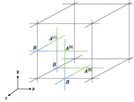
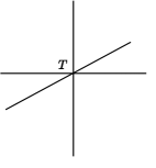
Figure 1: (Left) $A$ tensors on plaquettes and $B$ tensors on links. (Right) $T$ tensor in the center of a cube, where $T=A^{(0)}\otimes A^{(1)}\otimes A^{(2)}\otimes B\otimes B\otimes B$.

In what follows, we consider the SU(2) case and adopt Eq. (2.5) as the trial action. We truncate the bond dimension for $T$ to $D$ by introducing isometries as in the higher-order TRG(HOTRG) method Xie_2012 . The truncation procedure is summarized in Appendix A.

3 Numerical results

In this section we show the numerical results for three-dimensional SU(2) pure gauge theory on the lattice. We calculate the free energy (density) $F=(1/V)\log Z$ by using our formulation introduced in the previous section and the anisotropic TRG Adachi:2019paf . We adopt Eq. (2.5) with $N=2$ as the trial action $\tilde{S}_{v}$. In the following results, the lattice size $L$, which is related to $V$ as $V=L^{3}$, is fixed to $L=1024$.

First, by using the Monte Carlo method with the Boltzmann weight $e^{-\tilde{S}_{v}}$, we generate three sets of $K$ field configurations $G^{(i)}=\{U_{1}^{(i)},U_{2}^{(i)},\cdots,U_{K}^{(i)}\}\;(i=0,1,2)$. Second, we construct the $A^{(i)}$ tensors ($i=0,1,2$) from $G^{(i)}$ as explained in the previous section. Third, by installing isometries to truncate the bond dimension from $K^{2}$ to $D$ as explained in Appendix A, we construct the initial tensor $T$. Finally, we apply the ATRG Adachi:2019paf with the bond dimension $D$ to the initial tensor $T$ to calculate the free energy $F=\frac{1}{V}\log Z$. We perform the calculation of the free energy for various values of $H$ for fixed $\beta$ and search for a plateau of the free energy under the change of $H$ because the free energy is originally independent of $H$.

The estimates of the free energy have statistical errors in addition to the systematic errors coming from the finiteness of $K$ and the bond dimension $D$. The statistical errors that are given below as error bars are obtained from ten independent trials.

3.1 The $D$ and $K$ dependencies

In this subsection we examine the dependence of the free energy on $D$ and $K$. We choose $\beta=1$ and $\beta=50$ as typical values of small and large $\beta$, respectively.

First, we examine the $D$ dependence. The $D$ dependence of the free energy with $\beta=1$ and $\beta=50$ is shown in the left and right panels of Fig. 2, respectively. Here $K$ is fixed to $K=12$, and the results for two typical values of $H$ are shown. We see in Fig. 2 (left) that the statistical errors for $H=0.001$ are much smaller than those for $H=5$, and that the results for both $H=0.001$ and $H=5$ are stable against the change of $D$. We see in Fig. 2 (right) that the statistical errors for $H=20$ are much smaller than those for $H=1$, and the result for $H=20$ is stable against the change of $D$ while that for $H=1$ is not. These results imply that it is crucial in our algorithm to tune $H$ appropriately. In particular, $D=12$ is considered to be sufficient in both the weak and strong coupling regimes if $H$ is chosen appropriately.

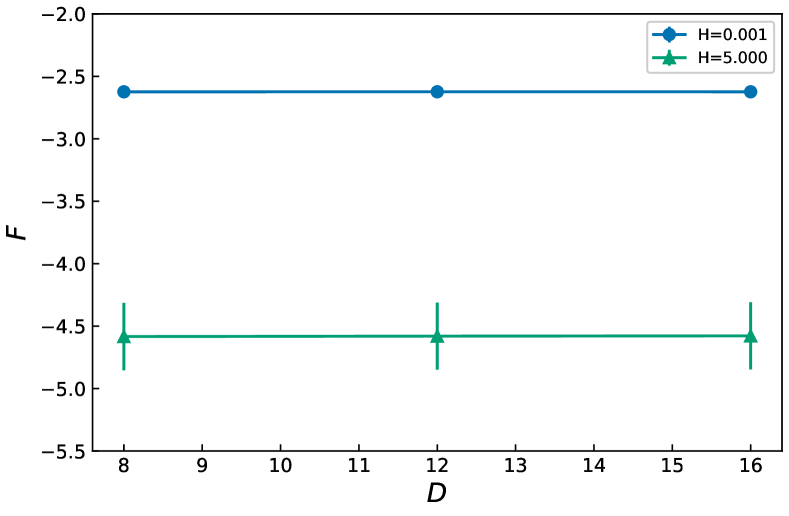
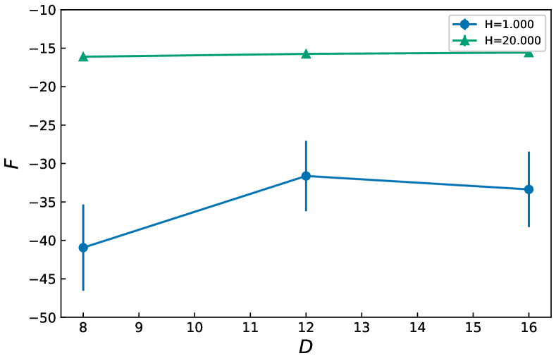
Figure 2: The $D$ dependence of the free energy with $\beta=1$ (left) and $\beta=50$ (right), where $K=12$. The lines are drawn to guide the eye. (Left) The dots and triangles represent the results for $H=0.001$ and $H=5$, respectively. The statistical errors for $H=0.001$ are smaller than the symbol size. (Right) The dots and triangles represent the results for $H=1$ and $H=20$, respectively. The statistical errors for $H=20$ are smaller than the symbol size.

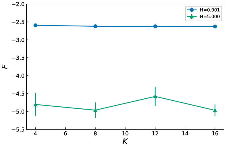
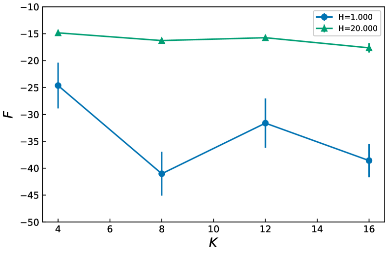
Figure 3: The $K$ dependence of the free energy with $\beta=1$ (left) and $\beta=50$ (right), where $D=12$. The lines are drawn to guide the eye. (Left) The dots and triangles represent the results for $H=0.001$ and $H=5$, respectively. The statistical errors for $H=0.001$ are smaller than the symbol size. (Right) The dots and triangles represent the results for $H=1$ and $H=20$, respectively. The statistical errors for $H=20$ are smaller than the symbol size.

Next, we examine the $K$ dependence. The $K$ dependence of the free energy with $\beta=1$ and $\beta=50$ is shown in the left and right panels of Fig. 3, respectively. Here, $D$ is fixed to $D=12$, and the results for two typical values of $H$ are shown. We see in Fig. 3 (left) that the statistical errors for $H=0.001$ are much smaller than those for $H=5$, and that the result for $H=0.001$ is stable against the change of $K$ while that for $H=5$ is not. This again implies that tuning $H$ is crucial in our algorithm, and $K=16$ is sufficient in the strong coupling regime. Similarly, we see in Fig. 3 (right) that the statistical errors for $H=20$ are much smaller than those for $H=1$. However, the result for $H=20$ does not look completely stable against the change of $K$ in the range $K\leq 16$. Due to the limitation of available memory, we take $K=16$ in the following calculations. Indeed, as we will show in Sect. 3.2, the result for the free energy for $20\leq\beta\leq 50$ agrees with the weak coupling expansion. Thus, the $K$ dependence for $K\geq 16$ with $H\sim 20$ is expected not to be large in the weak coupling regime. From the above results, we set $D=12$ and $K=16$ in the following calculations.

3.2 Free energy

We show the result for the free energy in Fig.4. Here $D$ and $K$ are fixed to $D=12$ and $K=16$ as mentioned in the previous subsection. We search for a plateau for each value of $\beta$ in the $0<H\leq 20$ region. The free energy is obtained from $F=F(H_{*})$, where $H_{*}$ has the smallest statistical error among the plateau. Note that $H_{*}$ depends on $\beta$. The dependence of the free energy on $H$ is shown in Fig. 5, where we choose $\beta=1$ and $\beta=50$ as typical small and large values of $\beta$, respectively. We see that there is a plateau in the $H\leq 0.6$ region for $\beta=1$ and in the $H\leq 16$ region for $\beta=50$. We take $H_{*}=0.001$ in $\beta\leq 7$ and $H_{*}>10$ in $\beta\geq 20$. ($H=0$ should also work for $\beta\leq 7$.)

The strong coupling expansion of the free energy is given by

$$F(\beta)=-3\beta+\frac{3}{8}\beta^{2}-\frac{3}{384}\beta^{4}+\mathcal{O}(\beta^{6})\ ,$$ (3.1)

which is expressed by the dashed line in Fig. 4. The weak coupling expansion of the expectation value of a plaquette is given by $W_{1\times 1}=e^{-1/\beta}$ Muller:1980hz . Thus we have

$$F(\beta)=-3\log\beta+C+\mathcal{O}\left(\frac{1}{\beta}\right)$$ (3.2)

with $C$ being an integration constant. We determine the constant $C$ as $C=-5.8426$ by fitting the data in the $20\leq\beta\leq 50$ region to $-3\log\beta+C$. The weak coupling expansion is expressed by the dotted line in Fig. 4. The result indeed agrees with the strong and weak coupling expansion, in the strong and weak regimes, respectively. However, in the $7\leq\beta\leq 19$ region, we cannot find any definite plateau. We expect this to be resolved by increasing $K$ and/or improving the trial action.

Our result suggests that the random sampling method Fukuma:2021cni works in the strong coupling regime in higher-dimensional gauge theories. If $K$ cannot be made large enough, another method is needed in the intermediate and weak coupling regimes. Our method is a candidate for such a method.

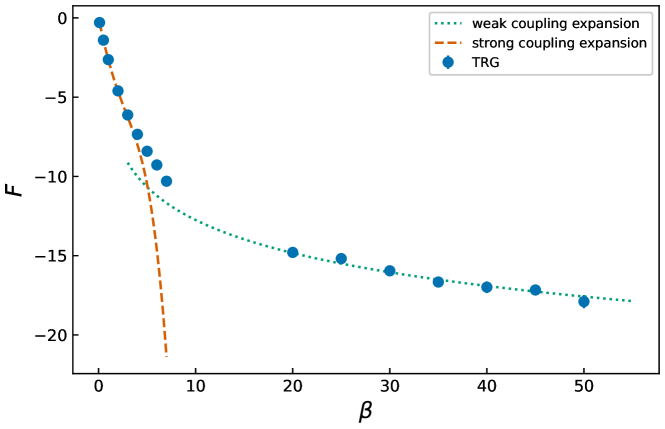
Figure 4: The free energy is plotted against $\beta$. The statistical errors are smaller than the symbol size. The strong coupling expansion is expressed by the dashed line, while the weak coupling expansion by the dotted line.

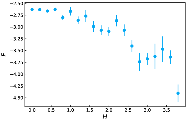
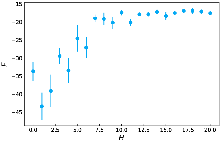
Figure 5: The $H$ dependence of the free energy with $K=16$ and $D=12$ for $\beta=1$(left) and $\beta=50$(right).

4 Conclusion and discussion

We proposed a method to represent the path integral over gauge fields as a tensor network. In our method, tensor indices label gauge field configurations that are generated with the weight determined by the trial action with variational parameters. We construct initial tensors with these indices and perform the TRG with the initial tensors for various values of the variational parameters to fix the variational parameters such that the result is insensitive to them. As a first step to the TRG study of non-Abelian gauge theories in more than two dimensions, we studied three-dimensional pure SU(2) gauge theory by using our method with the ATRG. We reproduced the weak and strong coupling behaviors of the free energy. We found that the random sampling method (corresponding to $H=0$) works in the strong coupling regime, while tuning $H$ to a nonzero value is needed in the weak coupling regime. Our result suggests that our method can be used for studying gauge theories in more than two dimensions.

It is likely that we need to perform the calculation with larger $K$ and/or to improve the trial action to see complete stability of the free energy against the change of $K$ in the weak and intermediate coupling regime. and find plateaus in the intermediate coupling regime

In order to establish the effectiveness of our method, we should study the physics of three-dimensional SU(2) gauge theory such as the string tension and the finite-temperature phase transitionKuramashi:2018mmi . Furthermore, inclusion of matter, topological terms, the chemical potential, extension to other non-Abelian gauge groups, and extension to four dimensions are left as future work. We hope that our method will indeed be powerful for problems with complex actions.

Appendix A Construction of the initial tensor

In this appendix we describe the details of the construction of the initial tensor. We have three $A$ tensors $\{A^{(0)},A^{(1)},A^{(2)}\}$ and three $B$ tensors that were introduced in Sect. 2. If the initial $T$ tensor is constructed exactly, the six-rank tensor needs an $\mathcal{O}\left((K^{2})^{6}\right)$ memory footprint. For this reason, we install isometries to reduce the bond dimension from $K^{2}$ to $D$. We apply HOTRGXie_2012 to coarse-grain the $x$, $y$, and $z$ directions as shown in Fig. 6.

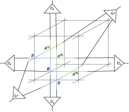
Figure 6: Isometries $U_{x}$, $U_{y}$, and $U_{z}$ for $x$, $y$, and $z$ directions, respectively.

First, we introduce the isometries for the $x$ direction. We perform higher-order singular value decomposition for $M\equiv A^{(0)}\otimes A^{(1)}\otimes B$. $M$ is a matrix whose rows consist of the indices of $A^{(0)}$ and $A^{(2)}$ corresponding to the right side (see Fig. 7) and the columns consist of the other indices (see Fig. 7) .

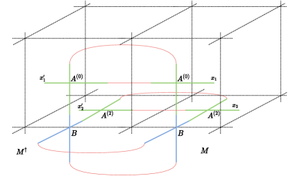
Figure 7: Coarse-graining for the $x$ direction. We consider the indices of $A^{(0)}$ and $A^{(2)}$, $(x_{1},x_{2})$, as the rows of the matrix $M$. We calculate $MM^{\dagger}$ by making the contractions expressed by the red lines.

Then, we calculate $MM^{\dagger}$, which is a Hermitian matrix, and perform the canonical transformation of $MM^{\dagger}$ as

$$MM^{\dagger}=U_{R}\Lambda_{R}(U_{R})^{\dagger}\ ,$$ (A.1)

where $\Lambda_{R}$ is a diagonal matrix whose diagonal elements are the eigenvalues of $MM^{\dagger}$. We also obtain $U_{L}$ for the left side in the same way. We can evaluate the truncation error $\epsilon_{R}$ and $\epsilon_{L}$ for $U_{R}$ and $U_{L}$:

$$\epsilon_{R(L)}=\sum_{i>D}(\Lambda_{R(L)})_{ii}\ .$$ (A.2)

We adopt the one with the smaller truncation error between $U_{R}$ and $U_{L}$ as $U_{x}$. $U_{y}$ and $U_{z}$ for the $y$ and $z$ directions are obtained in the same way: $M=A^{(0)}\otimes A^{(1)}\otimes B$ for the $y$ direction, and $M=A^{(1)}\otimes A^{(2)}\otimes B$ for the $z$ direction. Finally, we obtain the initial tensor $T$ by contracting $A^{(0)}$, $A^{(1)}$, $A^{(2)}$, $B$, $B$, $B$, $U_{x}$, $U_{y}$, and $U_{z}$ as in Fig. 6.

References

- (1) M. Levin and C. P. Nave, “Tensor renormalization group approach to 2D classical lattice models”, Phys. Rev. Lett., 99(12), 120601 (2007), cond-mat/0611687.
- (2) Y. Liu, Y. Meurice, M. P. Qin, J. Unmuth-Yockey, T. Xiang, Z. Y. Xie, J. F. Yu, and H. Zou, “Exact Blocking Formulas for Spin and Gauge Models”, Phys. Rev. D, 88, 056005 (2013), arXiv:1307.6543.
- (3) Z. Y. Xie, J. Chen, M. P. Qin, J. W. Zhu, L. P. Yang, and T. Xiang, “Coarse-graining renormalization by higher-order singular value decomposition”, Physical Review B, 86(4) (jul 2012).
- (4) Y. Shimizu and Y. Kuramashi, “Grassmann tensor renormalization group approach to one-flavor lattice Schwinger model”, Phys. Rev. D, 90(1), 014508 (2014), arXiv:1403.0642.
- (5) Y. Shimizu and Y. Kuramashi, “Critical behavior of the lattice Schwinger model with a topological term at using the Grassmann tensor renormalization group”, Phys. Rev. D, 90(7), 074503 (2014), arXiv:1408.0897.
- (6) Y. Shimizu and Y. Kuramashi, “Berezinskii-Kosterlitz-Thouless transition in lattice Schwinger model with one flavor of Wilson fermion”, Phys. Rev. D, 97(3), 034502 (2018), arXiv:1712.07808.
- (7) N. Butt, S. Catterall, Y. Meurice, R. Sakai, and J. Unmuth-Yockey, “Tensor network formulation of the massless Schwinger model with staggered fermions”, Phys. Rev. D, 101(9), 094509 (2020), arXiv:1911.01285.
- (8) S. Takeda and Y. Yoshimura, “Grassmann tensor renormalization group for the one-flavor lattice Gross–Neveu model with finite chemical potential”, PTEP, 2015(4), 043B01 (2015), arXiv:1412.7855.
- (9) S. Akiyama, Y. Kuramashi, T. Yamashita, and Y. Yoshimura, “Restoration of chiral symmetry in cold and dense Nambu–Jona-Lasinio model with tensor renormalization group”, JHEP, 01, 121 (2021), arXiv:2009.11583.
- (10) D. Kadoh, Y. Kuramashi, Y. Nakamura, R. Sakai, S. Takeda, and Y. Yoshimura, “Tensor network analysis of critical coupling in two dimensional theory”, JHEP, 05, 184 (2019), arXiv:1811.12376.
- (11) D. Kadoh, Y. Kuramashi, Y. Nakamura, R. Sakai, S. Takeda, and Y. Yoshimura, “Investigation of complex theory at finite density in two dimensions using TRG”, JHEP, 02, 161 (2020), arXiv:1912.13092.
- (12) S. Akiyama, D. Kadoh, Y. Kuramashi, T. Yamashita, and Y. Yoshimura, “Tensor renormalization group approach to four-dimensional complex theory at finite density”, JHEP, 09, 177 (2020), arXiv:2005.04645.
- (13) S. Akiyama, Y. Kuramashi, and Y. Yoshimura, “Phase transition of four-dimensional lattice 4 theory with tensor renormalization group”, Phys. Rev. D, 104(3), 034507 (2021), arXiv:2101.06953.
- (14) M. Asaduzzaman, S. Catterall, and J. Unmuth-Yockey, “Tensor network formulation of two dimensional gravity”, Phys. Rev. D, 102(5), 054510 (2020), arXiv:1905.13061.
- (15) A. Bazavov, S. Catterall, R. G. Jha, and J. Unmuth-Yockey, “Tensor renormalization group study of the non-Abelian Higgs model in two dimensions”, Phys. Rev. D, 99(11), 114507 (2019), arXiv:1901.11443.
- (16) M. Fukuma, D. Kadoh, and N. Matsumoto, “Tensor network approach to two-dimensional Yang–Mills theories”, PTEP, 2021(12), 123B03 (2021), arXiv:2107.14149.
- (17) M. Hirasawa, A. Matsumoto, J. Nishimura, and A. Yosprakob, “Tensor renormalization group and the volume independence in 2D U(N) and SU(N) gauge theories”, JHEP, 12, 011 (2021), arXiv:2110.05800.
- (18) Y. Kuramashi and Y. Yoshimura, “Three-dimensional finite temperature Z2 gauge theory with tensor network scheme”, JHEP, 08, 023 (2019), arXiv:1808.08025.
- (19) S. Akiyama and Y. Kuramashi, “Tensor renormalization group study of (3+1)-dimensional 2 gauge-Higgs model at finite density”, JHEP, 05, 102 (2022), arXiv:2202.10051.
- (20) D. Kadoh, Y. Kuramashi, Y. Nakamura, R. Sakai, S. Takeda, and Y. Yoshimura, “Tensor network formulation for two-dimensional lattice = 1 Wess-Zumino model”, JHEP, 03, 141 (2018), arXiv:1801.04183.
- (21) H. Kawauchi and S. Takeda, “Tensor renormalization group analysis of CP(N-1) model”, Phys. Rev. D, 93(11), 114503 (2016), arXiv:1603.09455.
- (22) S. Akiyama and D. Kadoh, “More about the Grassmann tensor renormalization group”, JHEP, 10, 188 (2021), arXiv:2005.07570.
- (23) D. Adachi, T. Okubo, and S. Todo, “Anisotropic Tensor Renormalization Group”, Phys. Rev. B, 102(5), 054432 (2020), arXiv:1906.02007.
- (24) D. Kadoh and K. Nakayama, “Renormalization group on a triad network” (12 2019), arXiv:1912.02414.
- (25) D. Kadoh, H. Oba, and S. Takeda, “Triad second renormalization group”, JHEP, 04, 121 (2022), arXiv:2107.08769.
- (26) Y. Kuramashi and Y. Yoshimura, “Tensor renormalization group study of two-dimensional U(1) lattice gauge theory with a term”, JHEP, 04, 089 (2020), arXiv:1911.06480.
- (27) J. Nishimura, T. Okubo, and F. Sugino, “Testing the Gaussian expansion method in exactly solvable matrix models”, JHEP, 10, 057 (2003), hep-th/0309262.
- (28) V. F. Muller and W. Ruhl, “Small Coupling (Low Temperature) Expansions of Gauge Field Models on a Lattice. Part 2. Expansions for the Gauge Group SU(2), the Regularization Problem of the Temporal Gauge Green’s Function” (5 1980).