Control of Dynamic Financial Networks
(The Extended Version)

Abstract

The current global financial system forms a highly interconnected network where a default in one of its nodes can propagate to many other nodes, causing a catastrophic avalanche effect. In this paper we consider the problem of reducing the financial contagion by introducing some targeted interventions that can mitigate the cascaded failure effects. We consider a multi-step dynamic model of clearing payments and introduce an external control term that represents corrective cash injections made by a ruling authority. The proposed control model can be cast and efficiently solved as a linear program. We show via numerical examples that the proposed approach can significantly reduce the default propagation by applying small targeted cash injections.

I Introduction

In this paper we consider the problem of mitigating the effects of financial contagion via targeted and optimized interventions. Recent studies [1, 2, 3, 4] highlighted the fact that in the current highly interconnected financial system, where banks and other institutions are linked via a network of mutual liabilities, a financial shock in one or few nodes of the network may hinder the possibility for these nodes to fulfill their obligations towards other nodes, and therefore provoke default. In turn, the nodes directly connected to the nodes that experienced the initial shocks receive reduced or no payments from these latter nodes, so their cash balances may be affected to the point of making impossible the fulfillment of their liabilities, hence of provoking further defaults, and so on in a cascaded fashion. The described mechanism may spread over the network as a contagion, provoking a possibly disastrous sequence of avalanche failures and defaults.

In the mainstream approach to the study of default spreading in financial networks, see, e.g., [5, 3], the contagion develops instantaneously, and in the aftermath of the contagion the nodes agree to settle for a set of mutual payments called clearing payments that brings the network to a new equilibrium after the shock. However, the assumption that all payments are simultaneous is quite unrealistic. For this reason, recently some works [6, 7, 8, 9, 10, 11] proposed time-dynamic extensions of this model. In particular, in [12] we consider a multi-step setting, in which defaults at one stage do not freeze all financial operations. Instead, in case of defaulted nodes, the residual claims are carried over to the next period, and so on until the end of the considered horizon. We show in [12] that multi-stage clearing payments can be computed by solving recursively a sequence of LP problems, and that the multi-step setting may mitigate the cascaded failure effects by allowing shocks to be absorbed over time.

In this paper, we start from the setup of the multi-step model developed in [12] and introduce in the model an external control term representing corrective cash injections at nodes to be performed by a ruling authority. The rationale is that a ruling authority, perhaps public, may intervene with minimal and targeted cash injections at certain nodes in order to prevent catastrophic cascaded failure events. We show that such control problem can be cast and efficiently solved as a linear program, an we provide numerical evidence of the fact that small targeted interventions at selected nodes (i.e., selected by the control algorithm itself) may suffice to avoid disastrous system-wide failures whose costs may be much larger than the amount necessary to prevent them. The notion of external injections of cash to reduce the contagion has been already deeply investigated [13, 14, 15, 16], in particular in the works on systemic risk measures (see, e.g., [17, 18]). However, in most of the cases these models consider a single-step setting where all payments are simultaneous. Instead, [19] considers a multi-step setting as in the proposed control problem. However, [19] does not consider the presence of an external control term as in the proposed model. In addition, differently from the proposed problem, [19] also assumes that entities cannot pay other entities more than the cash they have on hand.

The paper is structured as follows. In Sec. II we introduce the Eisenberg-Noe single-period model of a networked financial system. Sec. III presents the proposed multi-step dynamic extension with an external control term. Sec. IV introduces the problem of controlling the financial network by optimal cash injection. Sec. V shows two numerical examples. Conclusions are drawn in Sec. VI.

II The Eisenberg-Noe model

We start by describing the classical Eisenberg-Noe model of a networked financial system. Consider $n$ financial nodes (banks) who are subject to mutual liabilities $\bar{p}_{ij}\geq 0$, where $\bar{p}_{ij}$ represents the payment due from node $i$ to node $j$. The interbank liabilities constitute the liability matrix $\bar{P}\in{{\mathbb{R}}^{n\times n}}$, such that $[\bar{P}]_{ij}=\bar{p}_{ij}$ for $i\neq j=1,\ldots,n$, and $[\bar{P}]_{ii}=0$ for $i=1,\ldots,n$. Also, nodes may receive cash from external entities, which are not part of the network, and we denote by $c\in{{\mathbb{R}}_{+}^{n}}$ the vector whose $i$th component $c_{i}\geq 0$ represents the total cash in-flow from the external entities to node $i$. Following the approach in [5] we further assume that payments towards external entities are made to a fictitious node that owes no liability to the other nodes (the corresponding row of liability matrix $\bar{P}$ is zero). In the Eisenberg-Noe model time plays no role; specifically, all settlements of liabilities are assumed to be executed simultaneously at the end of a fixed time period. In normal situations, at the end of the considered period each node $i$ is able to pay its liabilities in full, which means that each node $i$ receives an inflow of liquidity $\bar{\phi}_{i}^{{\mathrm{in}}}\doteq c_{i}+\sum\nolimits_{k\neq i}\bar{p}_{ki}$ and pays out its liabilities by a total amount of $\bar{p}_{i}\doteq\bar{\phi}_{i}^{{\mathrm{out}}}\doteq\sum\nolimits_{k\neq i}\bar{p}_{ik}$. A critical situation instead occurs when (due to, e.g., a drop in the external in-flow $c_{i}$) some bank $i$ cannot fully pay its debt. In this situation, the actual payments to other banks have to be less than their nominal due values $\bar{p}_{ij}$. We denote by $p_{ij}\in[0,\bar{p}_{ij}]$, $i\neq j=1,\ldots,n$, the actual inter-bank payments executed at the end of the period, which we collect in matrix $P\in{{\mathbb{R}}^{n,n}}$. Under the actual payments, the cash inflows and outflows at each node $i=1,\ldots,n$, are respectively $\phi_{i}^{{\mathrm{in}}}\doteq c_{i}+\sum\nolimits_{k\neq i}p_{ki}$, $p_{i}\doteq\phi_{i}^{{\mathrm{out}}}\doteq\sum\nolimits_{k\neq i}p_{ik}$. The vectors of inflows and outflows are thus

$$\phi^{{\mathrm{in}}}\doteq c+P^{\top}{\mathbf{1}},\quad\phi^{{\mathrm{out}}}\doteq p\doteq P{\mathbf{1}},$$ (1)

where ${\mathbf{1}}$ denotes a vector of ones. The nonnegative balance condition requires that $w\doteq\phi^{{\mathrm{in}}}-\phi^{{\mathrm{out}}}\geq 0$. A matrix of mutual payments $P$, with $0\leq P\leq\bar{P}$, is said to be admissible if $w\geq 0$. If the nominal liabilities $\bar{P}$ are admissible then payments $P=\bar{P}$ are such that all mutual obligations are met while maintaining the net worth of each node nonnegative, and no default arises. If instead $\bar{P}$ is not admissible, then some nodes are in default, and all nodes must agree on a different set of admissible payments $P$, which are upper bounded by $\bar{P}$, since no node should pay more than due. Moreover, when a node is in default, it must pay out all of its cash inflow to the creditor nodes: each node $i$ pays out $\bar{p}_{i}$ or pays out its whole inflow $\phi_{i}^{{\mathrm{in}}}$. Therefore, a clearing payment matrix $0\leq P\leq\bar{P}$ obeys the relation

$$P{\mathbf{1}}=\min(\bar{P}{\mathbf{1}},c+P^{\top}{\mathbf{1}}).$$ (2)

One clearing matrix $0\leq P\leq\bar{P}$ satisfying (2) can be found [20] by solving an optimization problem of the form

$$\min_{P}\,f(P),\quad\mbox{s.t.: }0\leq P\leq\bar{P},\;P{\mathbf{1}}\leq c+P^{\top}{\mathbf{1}},$$ (3)

where $f(P)$ is any decreasing function of the matrix argument $P$ on $[0,\bar{P}]$, that is, a function such that $\bar{P}\geq P^{(2)}>P^{(1)}\geq 0$, $P^{(2)}\neq P^{(1)}$, implies $f(P^{(2)})<f(P^{(1)})$. Possible choices for $f$ in (3) are for instance $f(P)=\|\bar{\phi}^{{\mathrm{in}}}-\phi^{{\mathrm{in}}}\|_{1}$ and $f(P)=\|\bar{\phi}^{{\mathrm{in}}}-\phi^{{\mathrm{in}}}\|_{2}^{2}$, where $\phi^{{\mathrm{in}}}(P)=c+P^{\top}{\mathbf{1}}$. The optimal solution of (3), however, is in general non unique.

In practice, payments under default are subject to further regulations. A commonly used “local fairness” rule is that the outstanding claims should be redistributed based on a proportionality (pro-rata) rule. We define the relative proportion of payment due nominally by node $i$ to node $j$ as

$$a_{ij}\doteq\left\{\begin{array}[]{ll}\displaystyle\frac{\bar{p}_{ij}}{\bar{p}_{i}}&\mbox{if }\bar{p}_{i}>0\\ 1&\mbox{if }\bar{p}_{i}=0\,\mbox{ and }i=j\\ 0&\mbox{otherwise}.\end{array}\right.$$ (4)

Computing these proportions for all $i,j$ we form the relative liability matrix $A=[a_{ij}]$. By definition, matrix $A$ is row-stochastic, that is $A{\mathbf{1}}={\mathbf{1}}$. The so called pro-rata rule imposes that payments are due in proportion to the rates fixed in matrix $A$, that is $p_{ij}=a_{ij}p_{i},\quad\forall i,j$, where $p_{i}$ is the out-flow defined in (1). Since $p\doteq P{\mathbf{1}}$, the pro-rata rule imposes a set of linear equality constraints on the entries of $P$, namely $P=\mbox{\rm diag}(P{\mathbf{1}})A=\mbox{\rm diag}(p)A$. Under the pro-rata rule, the full payment matrix $P$ is determined by vector $p$; problem (3) simplifies in this case to

$$\min_{P}\,f(p),\quad\mbox{s.t.: }0\leq p\leq\bar{p},\;p\leq c+A^{\top}p,$$ (5)

and it holds that for any decreasing $f$ the solution $p^{*}$ to (5) is unique and it represents a clearing vector, that is, it satisfies $p=\min(\bar{p},c+A^{\top}p)$, see e.g. [20, Lemma 1].

Even though most of the works on financial contagion impose the pro-rata rule, in this paper we consider also the more general case without such constraint. The non-proportional clearing mechanism can significantly reduce the impact of a financial shock [20, 19]. In addition, it may also be extended to promote virtuous behaviors such as rescue consortium [21].

III A multi-stage model with controls

As already observed, the default and clearing model discussed in the previous section, which coincides with the mainstream one studied in the literature [3], is a single-period model, meaning that the described process assumes that at one point in time (the end of a fixed period), all liabilities are claimed and due simultaneously, and that the entire network of banks becomes aware of the claims and possible defaults and instantaneously agrees on the clearing payments. All financial operations of defaulted nodes are frozen, which possibly induces propagation of the default to other neighboring nodes, in an avalanche fashion, see, e.g., [22]. In [12], we propose a dynamic multi-step model in which financial operations are allowed for a given number of time periods after the initial theoretical defaults (here named pseudo-defaults). In this way some nodes may actually recover and eventually manage to fulfill their obligations by the end of the allotted time horizon. We next describe the dynamic model from [12], and introduce into this model additional control inputs that were not considered in [12].

We consider a discrete time horizon $t=0,1,\ldots,T$, with periods of fixed duration (e.g., one day, or one month, etc.), where $T\geq 0$ represents the final time of the horizon. For brevity, denote ${\mathcal{T}}\doteq\{0,\ldots,T-1\}$. Throughout the text, a sequence of vectors or matrices $(f(t),\,t\in{\mathcal{T}})$ is denoted by

$$[f]\doteq(f(0),\ldots,f(T-1)).$$

Extending to the multi-stage case the basic model described in Section II, we let $\bar{P}(t)\in{{\mathbb{R}}^{n\times n}}$, and $P(t)\in{{\mathbb{R}}^{n\times n}}$, $t\in{\mathcal{T}}$ denote the nominal liabilities matrices and the actual payment matrices at time $t$, respectively. We let $c(t)=e(t)+u(t)\geq 0$ denote the sum of the vector $e(t)\geq 0$ of cash inflows at nodes from the external sector at time $t$, plus the vector $u(t)\geq 0$ of additional “control inflows” injected at nodes at time $t$ by the control authority. We further define $\bar{P}\doteq\bar{P}(0)$ as the matrix of initial liabilities, and we let the pro-rata matrix $A$ be defined as in (4) according to these initial liabilities. In this work we can deal indifferently with models with full payment matrices, or with matrices constrained by the pro-rata condition: in this latter case we shall simply include the linear equality constraint $P(t)=\mbox{\rm diag}(p(t))A$ on the payment matrices, where $p(t)\doteq P(t){\mathbf{1}}$. The net worth $w_{i}(t)$ of node $i$ at $t$ evolves in accordance to $w_{i}(t+1)=w_{i}(t)+\phi_{i}^{{\mathrm{in}}}(t)-\phi_{i}^{{\mathrm{out}}}(t)$, or, in the vector form,

$$w(t+1)=w(t)+c(t)+P^{\top}(t){\mathbf{1}}-P(t){\mathbf{1}},\quad t\in{\mathcal{T}}.$$ (6)

Similar to the single-period case discussed in Section II, the limited liability condition requires that $w(t)\geq 0$ at all $t$. It may therefore happen that a payment $p_{ij}(t)<\bar{p}_{ij}(t)$ in order to guarantee $w_{i}(t)\geq 0$. When this happens at some $t<T$, instead of declaring default and freezing the financial system, we allow operations to continue up to the final time $T$, updating the due payments according to the equation $\bar{p}_{ij}(t+1)=\alpha\left(\bar{p}_{ij}(t)-p_{ij}(t)\right)$, where $\alpha\geq 1$ is the interest rate applied on past due payments. This can be written as

$$\bar{P}(t+1)=\alpha\left(\bar{P}(t)-P(t)\right),\quad t\in{\mathcal{T}}.$$ (7)

The recursions (6) and (7) are initialized with $w(0)=0$, $\bar{P}(0)=\bar{P}$, where $\bar{P}$ is the initial liability matrix. The meaning of equation (7) is that if a due payment at $t$ is not paid in full, then the residual debt is added to the nominal liability for the next period, possibly increased by an interest factor $\alpha\geq 1$. This mechanism allows for a node which is technically in default at a time $t$ to continue operations and (possibly) repay its dues in subsequent periods. Notice that matrix $\bar{P}(t)$ is time-varying and depends on the actual payment matrices $P(0),\ldots,P(t-1)$; the final matrix $\bar{P}(T)$ contains the residual debts at the end of the final period.

The payment matrices $P(t)$ are subject to the constraints

$$0\leq P(t)\leq\bar{P}(t)\quad\forall t\in{\mathcal{T}},$$ (8)

$$P(t){\mathbf{1}}\leq w(t)+c(t)+P(t)^{\top}{\mathbf{1}}\quad\forall t\in{\mathcal{T}},$$ (9)

where (8) represents the requirement that actual payments never exceed the nominal liabilities, and (9) represents the requirement that $w(t+1)$, as given in (6), remains nonnegative at all $t$. Conditions (8), (9) can be made explicit by eliminating the variables $w(t)$ and $\bar{P}(t)$, which by using (6)–(7) can be expressed as

$$\bar{P}(t)=\alpha^{t}\bar{P}(0)-\sum\nolimits_{k=0}^{t-1}\alpha^{t-k}P(k),$$ (10)

$$w(t)=C(t-1)+\sum\nolimits_{k=0}^{t-1}\left(P^{\top}(k)-P(k)\right){\mathbf{1}},$$ (11)

$$C(t)\doteq\sum\nolimits_{k=0}^{t}c(k)=\sum\nolimits_{k=0}^{t}[e(k)+u(k)].$$ (12)

Conditions (8), (9) can thus be rewritten as

$$P(t)\geq 0,\;\;\forall t\in{\mathcal{T}}$$ (13)

$$\sum\nolimits_{k=0}^{t}\alpha^{t-k}P(k)\leq\alpha^{t}\bar{P}\;\;\forall t\in{\mathcal{T}}$$ (14)

$$C(t)+\sum\nolimits_{k=0}^{t}\left(P(k)^{\top}-P(k)\right){\mathbf{1}}\geq 0\;\forall t\in{\mathcal{T}}$$ (15)

In the case when pro-rata is enforced the above conditions can be rewritten in terms of the outflow vectors only:

$$p(t)\geq 0,$$ (16)

$$\sum\nolimits_{k=0}^{t}\alpha^{t-k}p(k)\leq\alpha^{t}\bar{p}$$ (17)

$$C(t)+\sum\nolimits_{k=0}^{t}\left(A^{\top}p(k)-p(k)\right)\geq 0$$ (18)

$$\forall t\in{\mathcal{T}},\quad\bar{p}\doteq\bar{P}{\mathbf{1}}.$$

We say that a payment sequence $[P]$ is feasible for a given $[c]$, if it satisfies (13)–(15). Analogously, under pro-rata, a sequence $[p]$ is feasible for given $[c]$, if it satisfies (16)–(18).

We now introduce a system-level cost criterion, based on the total difference between the nominal and actual payments at the nodes. We define the loss at period $t$ by

$$\delta(t) \doteq \sum_{i,j=1}^{n}\left(\bar{p}_{ij}(t)-p_{ij}(t)\right)={\mathbf{1}}^{\top}\left(\bar{P}(t)-P(t)\right){\mathbf{1}}.$$ (19)

Observe that $\delta(t)\geq 0$ for all $t$ and for any feasible $[P]$, and $\delta(t)=0$ if and only if $P(t)=\bar{P}(t)$, that is when no default occurs. Therefore, $\delta(t)$ can be taken as a measure of the effects of defaults at stage $t$. The overall cost function is then defined as the total loss over the time horizon

$$L([P])\doteq\sum_{t=0}^{T-1}\delta(t)=a_{0}{\mathbf{1}}^{\top}\bar{P}{\mathbf{1}}-\sum_{t=0}^{T-1}a_{t}{\mathbf{1}}^{\top}P(t){\mathbf{1}},$$ (20)

where we derive the second equality from (10) and define the constants $a_{0}>a_{1}>\ldots>a_{T-1}$ as

$$a_{t}\doteq\sum_{j=0}^{T-t-1}\alpha^{j}=\left\{\begin{array}[]{ll}\frac{\alpha^{T-t}-1}{\alpha-1},&\mbox{if }\alpha>1\\ T-t,&\mbox{if }\alpha=1.\end{array}\right.$$ (21)

Now, for fixed input flows $[c]$, the multi-stage clearing payments $[P^{*}]$, are defined as the optimal solution to

$$\min_{[P]}L([P])\quad\mbox{s.t.:}\;\eqref{eq.cond-p-1+}-\eqref{eq.cond-p-2a}.$$ (22)

Analogously, under the pro-rata rule, the clearing payments are defined via vectors $p^{*}(t)$, $t\in{\mathcal{T}}$ which solve the LP

$$\min_{[p]}L([p])\quad\mbox{s.t.:}\;\eqref{eq.cond-p-1++}-\eqref{eq.cond-p-2b},$$ (23)

where $p(t)=P(t){\mathbf{1}}$, and $L([p])\doteq a_{0}{\mathbf{1}}^{\top}\bar{p}-\sum_{t=0}^{T-1}a_{t}{\mathbf{1}}^{\top}p(t)$. The properties of the optimization problems (22) and (23) (which are in fact LP) have been studied in [12].

IV Multi-step control of the dynamic network

We next consider the problem of controlling the financial network by optimal injections of cash $[u]=(u(0),\ldots,u(T-1))$ at nodes. The cumulative amount of cash injected from $0$ to $t$ is

$$B(t)\doteq\sum_{\tau=0}^{t}{\mathbf{1}}^{\top}u(\tau),\quad t\in{\mathcal{T}}.$$ (24)

The control objective we propose to minimize is defined as

$$J([P],[u])=(1-\eta)L([P])+\eta{\mathbf{1}}^{\top}\bar{P}(T){\mathbf{1}}+\gamma B(T-1),$$ (25)

where $L([P])$ is given in (20), $\gamma\geq 0$ is a given penalty on the total control cash, and $\eta\in[0,1]$ is a weight on the terminal cost ($\bar{P}(T)=0$ if and only if there is no default at the terminal time). The control problem is then stated as

$$\min_{[P],[u]} J([P],[u])$$ (26)

s.t.: $$[P]\geq 0,\quad[u]\geq 0$$ (27)

$$\sum\nolimits_{k=0}^{t}\alpha^{t-k}P(k)\leq\alpha^{t}\bar{P},\;t\in{\mathcal{T}}$$

$$C(t)+\sum\nolimits_{k=0}^{t}\left(P(k)^{\top}-P(k)\right){\mathbf{1}}\geq 0,\;t\in{\mathcal{T}}$$ (28)

$$B(t)\leq F(t),\;t\in{\mathcal{T}}$$ (29)

where $C(t)$ is given by (12) for fixed $[e]$, and $F(t)\geq 0$ is a given nondecreasing sequence that represents the maximum budget available up to time $t$ for controlling the network.

Under the pro-rata rule the control problem simplifies to

$$\min_{[p],[u]} J([p],[u])$$ (30)

s.t.: $$[p]\geq 0,\quad[u]\geq 0$$ (31)

$$\sum\nolimits_{k=0}^{t}\alpha^{t-k}p(k)\leq\alpha^{t}\bar{p},\;t\in{\mathcal{T}}$$

$$C(t)+\sum\nolimits_{k=0}^{t}\left(A^{\top}p(k)-p(k)\right)\geq 0,\;t\in{\mathcal{T}}$$

$$B(t)\leq F(t),\;t\in{\mathcal{T}},$$

where the cost function is

$$J([p],[u])=(1-\eta)L([p])+\eta{\mathbf{1}}^{\top}\bar{p}(T)+\gamma B(T-1),$$ (32)

In the case where $\eta\in[0,1)$ (the loss accumulated over time is penalized) and $\gamma>0$ (the total control cash is penalized), the solutions to the problems (26) and (30) enjoy a number of important properties. Denote the optimal sequences of payment matrices and control inputs by $P^{*}(t)$ and $[u^{*}]$ respectively (in the problem (30) $P^{*}(t)=\mbox{\rm diag}(p^{*}(t))A$). To each optimal solution, we associate the sequences $p^{*}(t)=P^{*}(t){\mathbf{1}}$ and $[{\bar{P}}^{*}],[{\bar{p}}^{*}],[c^{*}],[w^{*}],[B^{*}],[\delta^{*}]$.

Lemma 1.

Let $\eta\in[0,1),\gamma>0$. Then, all optimal processes in problems (26) and (30) enjoy the following properties:

1. The absolute debt priority rule is respected:

   $$p^{*}_{i}(t)=\min\left(\bar{p}_{i}^{*}(t),w^{*}(t)+c^{*}_{i}(t)+\sum\nolimits_{j\neq i}p_{ji}^{*}(t)\right)$$ (33)

   for all $i=1,\ldots,n$ and $t\in{\mathcal{T}}$;

2. A bank utilizes the injected liquidity immediately by paying out all its balance: if $u_{i}^{*}(t)>0$, then $w_{i}^{*}(t+1)=0$ and, moreover, $w_{i}(s)=0\,\forall s\leq t$.

3. If $B^{*}(t_{*})<F(t_{*})$ at some period $t_{*}<T-1$, then no liquidity is injected after period $t_{*}$: $u^{*}(t)=0\,\forall t>t_{*}$.

Notice that the first property shows that the optimal clearing policy prohibits unnecessary deferrals of payments: bank $i$ pay out its liability $\bar{p}_{i}^{*}(t)$ as soon as this is possible.

Note also that if the whole control budget is available at $t=0$, i.e., $F(0)=\ldots=F(T-1)$, then we either have $t_{*}=0$ and $B^{*}(0)<F(0)$ or the whole budget is used at time $t=0$. In both situations, one obviously has $u^{*}(t)=0\,\forall t\geq 1$. Similarly, if $F(k)=\ldots=F(T-1)$, then there are no control actions after period $k$: $u^{*}(t)=0\,\forall t\geq k+1$.

IV-A Dealing with uncertainty in the external payments

In problem (30) we assumed that the whole stream $[e]=(e(0),\ldots,e(T-1))$ of cash inflows from the external sector to the nodes is precisely known in advance. In this section we consider instead a more realistic scenario in which the inflows are known only up to some interval of uncertainty. More precisely, we assume that

$$e(t)=\hat{e}(t)+d(t),\quad t=0,\ldots,T-1,$$

where $\hat{e}(t)\geq 0$ is the nominal predicted value of the external cash inflow at $t$, and $d(t)$ is an unpredictable uncertainty on this value, assumed to bounded in magnitude so that

$$|d_{i}(t)|\leq r_{i}(t)\doteq\epsilon(t)\hat{e}_{i}(t),\quad i=1,\ldots,n;\;t=0,\ldots,T-1,$$

where $\epsilon(t)\in(0,1)$ is the given relative error level at $t$. We let ${\mathcal{D}}$ denote the uncertainty set on $[d]$, that is ${\mathcal{D}}=\{[d]:|d_{i}(t)|\leq r_{i}(t),i=1,\ldots,n;t=0,\ldots,T-1\}$.

For simplicity of exposition and notation we treat here only the case of proportional payments, which simplifies the problem and allows us to deal only with vector variables $p(t)$ instead of matrix variables $P(t)$. The whole reasoning reported below, however, carries over to the matrix case with only formal and notational modifications.

The decision variables $[p],[u]$ of problem (30) are next assumed to be prescribed by a reactive policy that allows adjustments in consequence to deviation of the external inflows from their nominal values: for all $t\in{\mathcal{T}}$ we let

$$p(t) = \hat{p}(t)+\Theta(t)(e(t)-\hat{e}(t))=\hat{p}(t)+\Theta(t)d(t)$$ (34)

$$u(t) = \hat{u}(t)+\Gamma(t)(e(t)-\hat{e}(t))=\hat{u}(t)+\Gamma(t)d(t).$$

and $[\hat{p}],[\hat{u}]$ are now the new decision variables, together with the collections of reaction matrices $[\Theta],[\Gamma]$. The control problem (30) is now cast in a worst-case setting as follows

$$\min_{[\hat{p}],[\hat{u}],[\Theta],[\Gamma]} \max_{[d]\in{\mathcal{D}}}J([p],[u])$$ (35)

s.t.: $$\min_{[d]\in{\mathcal{D}}}[p]\geq 0,\quad\min_{[d]\in{\mathcal{D}}}[u]\geq 0$$

$$\max_{[d]\in{\mathcal{D}}}\sum\limits_{k=0}^{t}\alpha^{t-k}p(k)\leq\alpha^{t}\bar{p},\,t\in{\mathcal{T}}$$

$$\min\limits_{[d]\in{\mathcal{D}}}C(t)+\sum\limits_{k=0}^{t}\left(A^{\top}p(k)-p(k)\right)\geq 0,\,t\in{\mathcal{T}}$$

$$\max_{[d]\in{\mathcal{D}}}B(t)\leq F(t),\;t\in{\mathcal{T}}.$$

The worst-case quantities appearing in problem (35) can be evaluated explicitly as reported next; in the omitted derivations we use repeatedly the fact that $\min_{|g|\leq r}h^{\top}g=-|h|^{\top}r$ and $\max_{|g|\leq r}h^{\top}g=|h|^{\top}r$:

$$\underline{p}(t) \doteq\min_{|d(t)|\leq r(t)}p(t)=\hat{p}(t)-|\Theta(t)|r(t)$$

$$\underline{u}(t) \doteq\min_{|d(t)|\leq r(t)}u(t)=\hat{u}(t)-|\Gamma(t)|r(t)$$

$$\bar{B}(t) \doteq\max_{[d]\in{\mathcal{D}}}B(t)=$$

$$=\sum\nolimits_{\tau=0}^{t}\left({\mathbf{1}}^{\top}\hat{u}(\tau)+{\mathbf{1}}^{\top}|\Gamma(\tau)|r(\tau)\right)$$

$$\bar{J}([\hat{p}],[\hat{u}],[\Theta],[\Gamma]) \doteq\max_{[d]\in{\mathcal{D}}}J([p],[u])$$

$$=J([\hat{p}],[\hat{u}])+$$

$$+\sum\nolimits_{t=0}^{T-1}{\mathbf{1}}^{\top}|\beta_{t}\Theta(t)+\gamma\Gamma(t)|r(t)$$

$$\underline{w}(t+1) \doteq\hat{w}(t+1)+$$

$$-\sum\nolimits_{k=0}^{t}|I+\Gamma(k)+(A^{\top}-I)\Theta(k)|r(k),$$

where for each $t\in{\mathcal{T}}$ one has

$$\beta_{t} \doteq\eta\alpha^{T-t}+(1-\eta)a_{t}$$

$$J([\hat{p}],[\hat{u}]) \doteq\beta_{0}{\mathbf{1}}^{\top}\bar{p}-\sum_{t=0}^{T-1}\beta_{t}{\mathbf{1}}^{\top}\hat{p}(t)+\gamma\sum_{t=0}^{T-1}{\mathbf{1}}^{\top}\hat{u}(t),$$

$$\hat{w}(t+1) \doteq\sum_{k=0}^{t}\left(\hat{e}(k)+\hat{u}(k)+A^{\top}\hat{p}(k)-\hat{p}(k)\right).$$

With the above positions, we can state the following

Proposition 1.

The finite-horizon robust control problem (35) is equivalent to the explicit linear program

$$\min_{[\hat{p}],[\hat{u}],[\Theta],[\Gamma]} \bar{J}([\hat{p}],[\hat{u}],[\Theta],[\Gamma])$$ (36)

s.t.: $$[\underline{p}]\geq 0,\quad[\underline{u}]\geq 0$$

$$\sum\nolimits_{k=0}^{t}\alpha^{t-k}\left(\hat{p}(k)+|\Theta(k)|r(k)\right)\leq\alpha^{t}\bar{p},\;t\in{\mathcal{T}}$$

$$\underline{w}(t+1)\geq 0,\;t\in{\mathcal{T}}$$

$$\bar{B}(t)\leq F(t),\;t\in{\mathcal{T}}.$$

V Numerical illustration

To illustrate the proposed approach, we consider a schematic network with $6$ nodes, plus the external fictitious node, as shown in Figure 1.

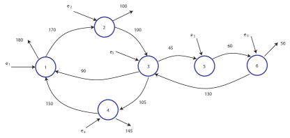
Figure 1: A schematic network with $6$ nodes.

The numbers on the edges in the graph in Figure 1 represent the initial nominal liabilities, forming the liability matrix $\bar{P}$, vector $e=(e_{1},\ldots,e_{6})$ represents the external cash inflows at the nodes. We assume that the proportionality rule for default payments is in force.

V-A Nominal control

Consider first a nominal scenario over a single period $T=1$, in which $\begin{smallmatrix}e(0)=(105,\,25,\,10,\,190,\,10,\,120,\,0)\end{smallmatrix}$. In this case, with no control, all nodes default. The clearing payments, computed according to (5), result to be

$$P(0)=\left[\begin{smallmatrix}0&164.6&0&0&0&0&174.3\\ 0&0&94.81&0&0&0&94.81\\ 86.18&0&0&100.5&43.09&0&0\\ 147.7&0&0&0&0&0&142.8\\ 0&0&0&0&0&53.09&0\\ 0&0&125.0&0&0&0&48.08\\ 0&0&0&0&0&0&0\end{smallmatrix}\right].$$

After such a clearing round, each node owes the residual amounts $(\begin{smallmatrix}11.08\;&10.38\;&10.18\;&4.45\;&6.91\;&6.91\;&0\end{smallmatrix})$, for a total loss of $49.92$. The question now is the following: what could be a control intervention that may avoid the default? To answer this question we solved the control problem (30), over a single period $T=1$, setting parameters $\eta=0.9$, $\gamma=1$, and a total control budget $F(0)=50$. The resulting optimal control action resulted to be $u(0)=(5,\;5,\;0,\;0,\;5,\;0)$. It can be readily checked that with such control action the total in-flows are $c(0)=e(0)+u(0)$, and for such inputs the network returns to regular operations, with no default. Overall, in this example, a relatively small intervention of amplitude $\|u(0)\|_{1}=15$ would be able to completely prevent the defaults and bring the losses to zero.

We next consider a multi-stage setup with $T=3$ periods. We assume a $1\%$ interest rate on residual payments (i.e., $\alpha=1.01$), and assume the following predicted stream of external payments

$$e(0)=\left[\begin{smallmatrix}105\\ 0\\ 10\\ 0\\ 0\\ 0\\ 0\end{smallmatrix}\right],e(1)=\left[\begin{smallmatrix}0\\ 25\\ 0\\ 190\\ 0\\ 0\\ 0\end{smallmatrix}\right],e(2)=\left[\begin{smallmatrix}0\\ 0\\ 0\\ 0\\ 10\\ 120\\ 0\end{smallmatrix}\right].$$

We use, as in the previous case, $\eta=0.9$, $\gamma=1$, and we assume that the total control budget of $50$ is available progressively as $F(0)=15$, $F(1)=30$, $F(2)=50$. In this case, the solution of the control problem (30) gave us the optimal interventions

$$u(0)=\left[\begin{smallmatrix}2.19\\ 5.25\\ 0\\ 0\\ 5.20\\ 2.36\\ 0\end{smallmatrix}\right],u(1)=\left[\begin{smallmatrix}2.84\\ 0\\ 0\\ 1.9\\ 0\\ 0\\ 0\end{smallmatrix}\right],u(2)=0.$$

These optimal injections, together with the computed optimal payment matrices at the intermediate times, are such that the network arrives to a regular (i.e., non default) situation at $T=3$. The optimal payment vectors were

$$p(0)=\left[\begin{smallmatrix}143.82\\ 75.11\\ 61.32\\ 26.83\\ 16.69\\ 19.06\\ 0\end{smallmatrix}\right],\;p(1)=\left[\begin{smallmatrix}131.04\\ 88.65\\ 51.27\\ 214.33\\ 9.61\\ 9.61\\ 0\end{smallmatrix}\right],\;p(2)=\left[\begin{smallmatrix}77.96\\ 37.87\\ 130.49\\ 57.09\\ 34.47\\ 154.47\\ 0\end{smallmatrix}\right].$$

The full payment matrices can be deduced from the above payment vectors via the relation $P(t)=\mbox{\rm diag}(p(t))A$, where $A$ is the pro-rata matrix

$$A=\left[\begin{smallmatrix}0&0.4857&0&0&0&0&0.5143\\ 0&0&0.5&0&0&0&0.5\\ 0.375&0&0&0.4375&0.1875&0&0\\ 0.5085&0&0&0&0&0&0.4915\\ 0&0&0&0&0&1.0&0\\ 0&0&0.7222&0&0&0&0.2778\\ 0&0&0&0&0&0&1\end{smallmatrix}\right].$$

The control effort in the present case amounts to a total ${\mathbf{1}}^{\top}(u(0)+u(1)+u(2))=19.74$, which is higher than the control effort needed in the single-stage case. This is expected since, due to interest, there is a price to pay for not having all the external payments available at $t=0$, and making the total control budget available only partially at the intermediate stages.

V-B Robust control

We now examine the case of uncertain input flows. We discuss first a single-step case ($T=1$). Consider the nominal input cash flow $\hat{e}(0)=(158,\,38,\,15,\,285,\,15,\,180,\,0)$. In this nominal situation, the network is in regular operation, all payments meet their liabilities, no default occurs, and no corrective control action is needed. Assume, however, that the actual inputs are not exactly known, being however within a $33\%$ interval from the nominal values. By solving the robust control problem (36) with $\eta=0.9$, $\gamma=1$, and $F(0)=50$, we obtain that the optimal policies (34) are able to maintain the system default free in the worst case. This is achieved via the nominal control action and nominal payment

$$\hat{u}(0)=\left[\begin{smallmatrix}1.32\\ 1.49\\ 0.61\\ 0.13\\ 1.31\\ 0.65\\ 0.0\end{smallmatrix}\right],\quad\hat{p}(0)=\left[\begin{smallmatrix}348.69\\ 198.52\\ 239.40\\ 294.87\\ 58.70\\ 179.35\\ 0.0\end{smallmatrix}\right],$$

and reaction matrices

$$\Theta(0) = \left[\begin{smallmatrix}23&1.8&6.5&0.22&2.8&0.32&0\\ 5&95&1.1&0.049&0.46&0.054&0\\ 1.1&13&38&0.011&16&1.8&0\\ 0.11&0.75&1.9&0.93&1.7&0.16&0\\ 0.086&1&3.1&0&250&0.13&0\\ 0.029&0.34&1&0&55&6&0\\ 0&0&0&0&0&0&0\end{smallmatrix}\right]\times 10^{-3},$$

$$\Gamma(0) = \left[\begin{smallmatrix}-23&-1.8&-6.6&-0.22&-2.8&-0.32&0\\ -5.0&-96&-1.1&-0.049&-0.47&-0.055&0\\ -1.1&-13&-39&-0.011&-16&-1.8&0\\ -0.11&-0.75&-2&-0.93&-1.7&-0.16&0\\ -0.087&-1&-3.1&0&-250&-0.13&0\\ -0.029&-0.34&-1&0&-55&-6.1&0\\ 0&0&0&0&0&0&0\end{smallmatrix}\right]\times 10^{-3}.$$

We finally consider a multi-step situation with $T=3$ and nominal external in-flows

$$\hat{e}(0)=\left[\begin{smallmatrix}15\\ 30\\ 10\\ 200\\ 5\\ 100\\ 0\end{smallmatrix}\right],\hat{e}(1)=\left[\begin{smallmatrix}80\\ 4\\ 0\\ 40\\ 5\\ 40\\ 0\end{smallmatrix}\right],\hat{e}(2)=\left[\begin{smallmatrix}63\\ 4\\ 5\\ 45\\ 5\\ 40\\ 0\end{smallmatrix}\right].$$

We assume that the external flow has 10% uncertainty at $t=0$, while the ucertainty rises to 33% at $t=1$ and $t=2$. We let $\eta=0.9$, $\gamma=1$, $\alpha=1.01$, and $F(0)=15$, $F(1)=30$, $F(2)=50$. Solving (36) gives optimal policies that guarantee that the system is default free at the final time $T$, in all possible scenarios. The control effort was equal to $3.9$ in the nominal scenario and to $4.87$ in the worst-case scenario, meaning that at most this sum is spent by the regulatory authority to maintain the system free of defaults.

VI Conclusions

In this paper, we proposed a multi-period financial network model with an external control term representing corrective cash injections that can be performed by a ruling authority in order to prevent catastrophic cascaded failure events. We studied both the nominal case, in which the cash inflows from the external sector are precisely known in advance, and the more realistic case where the inflows are known only up to some interval of uncertainty. In this latter case, we proposed a robust approach based on linear feedback policies. In all the considered scenarios, the proposed control problems turn out to be efficiently solvable by means of linear programming. Numerical examples support the claim that small targeted interventions may avoid a cascaded failure effect and may thus significantly reduce the interbank contagion.

Proof of Lemma 1

Statement 1

To prove the first statement of Lemma, we first notice that if $([P^{*}],[u^{*}])$ is an optimal solution in (26), then $[P^{*}]$ is an optimal solution in the problem

$$\min_{[P]} J([P],[u^{*}])$$ (37)

s.t.: $$[P]\geq 0,$$

$$\sum\nolimits_{k=0}^{t}\alpha^{t-k}P(k)\leq\alpha^{t}\bar{P},\;t\in{\mathcal{T}}$$

$$C^{*}(t)+\sum\nolimits_{k=0}^{t}\left(P(k)^{\top}-P(k)\right){\mathbf{1}}\geq 0,\;t\in{\mathcal{T}}$$

(where $C^{*}(t)=c^{*}(0)+\ldots+c^{*}(t)$ corresponds to fixed control inputs $c^{*}(t)=e(t)+u^{*}(t)$, and the only decision variable is the sequence of payment matrices $[P]$).

Similarly, if $([p^{*}],[u^{*}])$ is an optimal solution in (30), then $[p^{*}]$ is an optimal solution in the problem

$$\min_{[p]} J([p],[u^{*}])$$ (38)

s.t.: $$[p]\geq 0,$$

$$\sum\nolimits_{k=0}^{t}\alpha^{t-k}p(k)\leq\alpha^{t}\bar{p},\;t\in{\mathcal{T}}$$

$$C^{*}(t)+\sum\nolimits_{k=0}^{t}\left(A^{\top}p(k)-p(k)\right)\geq 0,\;t\in{\mathcal{T}}$$

Recalling the definition of cost functions (25) and (32), one notices that the final budget $B(T-1)=B^{*}(T-1)$ is now also fixed, and hence $J$ in (37) (respectively, (38)) can be replaced by

$$\tilde{L}([P])=(1-\eta)L([P])+\eta{\mathbf{1}}^{\top}\bar{P}(T){\mathbf{1}},$$

or, respectively,

$$\tilde{L}([p])=(1-\eta)L([p])+\eta{\mathbf{1}}^{\top}\bar{p}(T).$$

The first statement of Lemma 1 (absolute priority rule) is now implied by [12, Theorem 1] (in the case of free payments) and [12, Theorem 1] (in the case of pro-rata payments). Note that formally Theorems 1 and 2 in [12] are formulated for the special case $\eta=0$, where $\tilde{L}=L$ coincides with the total loss (20). However, as noted in [12, Appendix A.4], these theorems hold also for $\eta\in[0,1)$. $\star$

Statement 2

Notice that (33), in view of (6), can be rewritten as follows: if $p_{i}(t)<\bar{p}_{i}^{*}(t)$ (some debt remains unpaid by period $t$), then $w_{i}^{*}(t)=0$. To prove the second statement, notice now that the banks whose liability has been paid by period $t$ (that is, $\bar{p}_{i}^{*}(t)=0$), obviously, do not receive additional cash at periods $t,t+1,\ldots,T-1$: otherwise, one could reduce the total budget $B(T-1)$ without violating any constraint. Hence, if $u_{i}^{*}(t)>0$, then some debt remained unpaid ($p_{i}^{*}(s)<\bar{p}_{i}^{*}(s)$) at all periods $s=0,\ldots,t-1$, which, as has been noted, entails that $w_{i}^{*}(0)=\ldots=w_{i}^{*}(t)=0$. It remains to prove that $w_{i}^{*}(t+1)=0$, which will now be proved by contradiction. Assume that $w_{i}^{*}(t+1)>0$. In view of (33), one has

$$w_{i}^{*}(t)+e_{i}^{*}(t)+u_{i}^{*}(t)+\sum_{j\neq i}p_{ji}^{*}(t)>\bar{p}_{i}^{*}(t).$$

The latter inequality, however, remains valid if one reduces $u_{i}^{*}(t)$ by a small constant, decreasing thus also the total amount of case $B(T-1)$ and the value of cost function $J$. This contradicts to the solution’s optimality. $\star$

Statement 3

Note first that statement 3 follows from a formally weaker statement (A):

(A) For every optimal solution to the problem (26) or problem (30) and every instant $t_{0}<T-1$ the implication holds: if $B^{*}(t_{0})<F(t_{0})$ (the budget constraint is not active at $t=t_{0}$), then $u^{*}(t_{0}+1)=0$.

Indeed, suppose that $B^{*}(t_{*})<F(t_{*})$ yet $u^{*}(t)\neq 0$ at some instant $t\geq t_{0}+1$; let $t_{1}$ be the first such instant. Then, $t_{1}>t_{*}+1$ (due to statement (A)) and $u^{*}(t_{*}+1)=\ldots=u^{*}(t_{1}-1)=0$. Therefore, $B^{*}(t_{1}-1)=B^{*}(t_{*})<F(t_{*})\leq F(t_{1}-1)$. Statement (A) applied to $t_{0}=t_{1}$ implies now that $u^{*}(t_{1})=0$, which contradicts to the choice of $t_{1}$.

Proof of Statement (A)

Assume that $B^{*}(t_{0})<F(t_{0})$ yet $u(t_{0}+1)\neq 0$. We will demonstrate that this assumption leads to the contradiction with the optimality of the solution, using the arguments similar to the “advanced payment transformations” from [12].

Consider first a simpler case of free payments (the problem (30)). Let $i$ be one of the banks that receive extra cash at time $t_{0}+1$: $u_{i}(t_{0}+1)>0$. Due to statement 2, this is possible only when $\bar{p}_{i}^{*}(t_{0}+1)>0$ and, furthermore, (33) implies (in view of $c_{i}^{*}(t_{0}+1)\geq u_{i}^{*}(t_{0}+1)>0$) that $p_{i}^{*}(t_{0}+1)>0$, so at least bank $j\neq i$ receives payment from $i$: $p_{ij}^{*}(t_{0}+1)>0$, and hence $p_{ij}^{*}(t_{0})<\bar{p}_{ij}^{*}(t_{0})$.

Define the sequence $[P]$ of payment matrices as follows

$$p_{km}(t)=\begin{cases}p_{ij}^{*}(t_{0})+\alpha^{-1}\varepsilon,&(i,j)=(k,m),t=t_{0},\\ p_{ij}^{*}(t_{0}+1)-\varepsilon,&(i,j)=(k,m),t=t_{0}+1,\\ p_{km}^{*}(t),&\text{in all other cases}.\end{cases}$$

and also a new sequence of control inputs $[u]$, where

$$u_{k}(t)=\begin{cases}u_{i}^{*}(t_{0})+\alpha^{-1}\varepsilon,&k=i,t=t_{0},\\ u_{i}^{*}(t_{0}+1)-\varepsilon,&k=i,t=t_{0}+1,\\ u^{*}_{j}(t_{0}+1)+(1-\alpha^{-1})\varepsilon,&k=j,\,t=t_{0}+1\\ u^{*}_{k}(t),&\text{in all other cases}.\end{cases}$$

In other words, $i$ pays to $j$ a larger amount at time $t=t_{0}$ in order to decrease the payment at time $t=t_{0}+1$. To make this possible without violating the inequality $w(t)\geq 0$, one has to increase the cash input injected to $i$ at time $t=t_{0}$ (to make and the cash input to $j$ at time $t=t_{0}+1$; at the same time, the cash input to $i$ at time $t=t_{0}$ have to be decreased in order to preserve the total budget. Here $\varepsilon>0$ is such that

$$\begin{gathered}p_{ij}(t_{0}+1)>0,u_{i}(t_{0}+1)>0,p_{ij}(t_{0})<\bar{p}_{ij}^{*}(t_{0}),\\ B(t_{0})=B^{*}(t_{0})+\alpha^{-1}\varepsilon<F(t_{0}).\end{gathered}$$

By construction, $P(t),u(t)$ are nonnegative. One may also notice that $([P],[u])$ satisfy the conditions (27), (28) and (29). The condition (29) at time $t=t_{0}$ is guaranteed by the choice of $\varepsilon$, whereas $B(t)=B^{*}(t)\leq F(t)\,\forall t\neq t_{0}$.

The condition (27) is not violated for $t\neq t_{0}$, because the its left-hand side remains invariant after the replacement of $[P^{*}]$ by $[P]$. To verify this condition at $t=t_{0}$, recall that (27) is nothing else than the inequality $P(t)\leq\bar{P}(t)$, which holds at $t=t_{0}$ by construction.

The condition (28) is equivalent to the relation $w_{k}(t+1)\geq 0\,\forall k=1,\ldots,n$. It can be easily seen that, by construction, one has $w_{k}(t+1)=w_{k}^{*}(t+1)$ for all $k\neq j$, whereas

$$w_{j}(t+1)=\begin{cases}w_{j}^{*}(t+1),&t\neq t_{0}\\ w_{j}^{*}(t_{0}+1)+\alpha^{-1}\varepsilon>w_{j}^{*}(t_{0}+1),&t=t_{0}.\end{cases}$$

Hence, (28) also holds. At the same time,

$$J([P],[u])=J([P^{*}],[u^{*}])+(\alpha^{-1}a_{t_{0}}-a_{t_{0}+1})\varepsilon<J([P^{*}],[u^{*}]),$$

which leads us to the contradiction with the optimality of $([P^{*}],[u^{*}])$. Hence, the statement (A) is valid.

The case of pro-rata constraint is considered similarly with the only difference that, transferring the payment of bank $i$ from period $t_{0}+1$ to $t_{0}$, the control intervention at time $t=t_{0}+1$ is needed by all banks $j\neq i$. Instead of sequence of matrices $[P]$, one can construct a sequences of payment vectors $[p]$ by defining

$$p_{k}(t)=\begin{cases}p_{i}^{*}(t_{0})+\alpha^{-1}\varepsilon,&k=i\;\text{and}\;t=t_{0},\\ p_{i}^{*}(t_{0}+1)-\varepsilon,&k=i\;\text{and}\;t=t_{0}+1,\\ p_{k}^{*}(t),&\text{in all other cases}.\end{cases}$$

and a sequence of control inputs

$$u_{k}(t)=\begin{cases}u_{i}^{*}(t_{0})+\alpha^{-1}\varepsilon,&k=i,t=t_{0},\\ u_{i}^{*}(t_{0}+1)-\varepsilon,&k=i,t=t_{0}+1,\\ u^{*}_{k}(t_{0}+1)+(1-\alpha^{-1})\varepsilon a_{ik},&k\neq i,\,t=t_{0}+1\\ u^{*}_{k}(t),&\text{in all other cases}.\end{cases}$$

Here $\varepsilon>0$ is so small that $p_{i}(t_{0})<\bar{p}_{i}^{*}(t_{0})$, $p_{i}(t_{0}+1)>0$, $u_{i}^{*}(t_{0}+1)>0$ and $B(t_{0})=B^{*}(t_{0})+\alpha^{-1}\varepsilon<F(t_{0})$. It can be shown that $J([p],[u])<J([p^{*}],[u^{*}])$ and the pair of sequences $([p],[u])$ is feasible, in particular, $w_{k}(t+1)=w_{k}^{*}(t+1)$ for all $t\neq t_{0}$ and all $k$ and

$$w_{k}(t_{0}+1)=\begin{cases}w_{i}^{*}(t_{0}+1),&k=i\\ w_{k}^{*}(t_{0}+1)+\alpha^{-1}\varepsilon a_{jk}>w_{k}^{*}(t_{0}+1),&k\neq i.\end{cases}$$

This leads to the contradiction with optimality of $([p^{*}],[u^{*}])$. Statement (A) is proved. $\star$

References

- [1] D. M. Gale and S. Kariv, “Financial networks,” American Economic Review, vol. 97, no. 2, pp. 99–103, 2007.
- [2] S. Battiston, J. B. Glattfelder, D. Garlaschelli, F. Lillo, and G. Caldarelli, “The structure of financial networks,” in Network Science. Springer, 2010, pp. 131–163.
- [3] P. Glasserman and H. P. Young, “Contagion in financial networks,” Journal of Economic Literature, vol. 54, no. 3, pp. 779–831, 2016.
- [4] M. Elliott, B. Golub, and M. O. Jackson, “Financial networks and contagion,” American Economic Review, vol. 104, no. 10, pp. 3115–53, 2014.
- [5] L. Eisenberg and T. H. Noe, “Systemic risk in financial systems,” Management Science, vol. 47, no. 2, pp. 236–249, 2001.
- [6] I. M. Sonin and K. Sonin, “Banks as tanks: A continuous-time model of financial clearing,” arXiv preprint arXiv:1705.05943, 2017.
- [7] H. Chen, T. Wang, and D. D. Yao, “Financial network and systemic risk—a dynamic model,” Production and Operations Management, vol. 30, no. 8, pp. 2441–2466, 2021.
- [8] T. Banerjee, A. Bernstein, and Z. Feinstein, “Dynamic clearing and contagion in financial networks,” online as ArXiv:1801.02091, 2018.
- [9] A. Capponi and P.-C. Chen, “Systemic risk mitigation in financial networks,” Journal of Economic Dynamics and Control, vol. 58, pp. 152–166, 2015.
- [10] G. Ferrara, S. Langfield, Z. Liu, and T. Ota, “Systemic illiquidity in the interbank network,” Quantitative Finance, vol. 19, no. 11, pp. 1779–1795, 2019.
- [11] M. Kusnetsov and L. A. Maria Veraart, “Interbank clearing in financial networks with multiple maturities,” SIAM Journal on Financial Mathematics, vol. 10, no. 1, pp. 37–67, 2019.
- [12] G. Calafiore, G. Fracastoro, and A. Proskurnikov, “Clearing payments in dynamic financial networks,” Under review, 2021, online as ArXiv:2201.12898v4.
- [13] A. Minca and A. Sulem, “Optimal control of interbank contagion under complete information,” Statistics & Risk Modeling, vol. 31, no. 1, pp. 23–48, 2014.
- [14] H. Amini, A. Minca, and A. Sulem, “Control of interbank contagion under partial information,” SIAM Journal on Financial Mathematics, vol. 6, no. 1, pp. 1195–1219, 2015.
- [15] ——, “Optimal equity infusions in interbank networks,” Journal of Financial stability, vol. 31, pp. 1–17, 2017.
- [16] G. Fukker and C. Kok, “On the optimal control of interbank contagion in the euro area banking system,” ECB Working Paper, 2021.
- [17] Z. Feinstein, B. Rudloff, and S. Weber, “Measures of systemic risk,” SIAM Journal on Financial Mathematics, vol. 8, no. 1, pp. 672–708, 2017.
- [18] F. Biagini, J.-P. Fouque, M. Frittelli, and T. Meyer-Brandis, “A unified approach to systemic risk measures via acceptance sets,” Mathematical Finance, vol. 29, no. 1, pp. 329–367, 2019.
- [19] S. Barratt and S. Boyd, “Multi-period liability clearing via convex optimal control,” Available at SSRN 3604618, 2020.
- [20] G. Calafiore, G. Fracastoro, and A. Proskurnikov, “Optimal clearing payments in a financial contagion model,” Submitted, 2021, online as arXiv:2103.10872.
- [21] L. C. Rogers and L. A. Veraart, “Failure and rescue in an interbank network,” Management Science, vol. 59, no. 4, pp. 882–898, 2013.
- [22] L. Massai, G. Como, and F. Fagnani, “Equilibria and systemic risk in saturated networks,” Mathematics of Operation Research, 2021, published online, as arXiv:1912.04815.