Full Counting Statistics and Fluctuation Theorem for the Currents in the Discrete Model of Feynman’s Ratchet

Abstract

We provide a detailed investigation on the fluctuations of the currents in the discrete model of Feynman’s ratchet proposed by Jarzynski and Mazonka in 1999. Two macroscopic currents are identified, with the corresponding affinities determined using Schnakenberg’s graph analysis. We also investigate full counting statistics of the two currents and show that fluctuation theorem holds for their joint probability distribution. Moreover, fluctuation-dissipation relation, Onsager reciprocal relation and their nonlinear generalizations are numerically shown to be satisfied in this model.

I Introduction

Feynman’s ratchet and pawl system – a device capable of converting thermal random motion into useful work – acts as a microscopic mechanical Maxwell’s demon Feynman et al. (1965). As a paradigm for rectifying thermal noise, it has inspired extensive theoretical studies Magnasco (1993); Parrondo and Español (1996); Sekimoto (1997); Magnasco and Stolovitzky (1998); Astumian and Derényi (1998); VandenBroeck et al. (2004); Ryabov et al. (2016); Gomez-Marin and Sancho (2006); Nakagawa and Komatsu (2006); Tu (2008); Hondou and Takagi (1998); Komatsu and Nakagawa (2006); Skordos and Zurek (1992) as well as experimental efforts Martínez et al. (2017); Albay et al. (2018, 2020); Eshuis et al. (2010); Jun et al. (2014); Bérut et al. (2012); Toyabe and Sano (2015). Its basic setup includes a ratchet and a pawl (see Fig. 1). From time to time, the pawl switches between being engaged and disengaged. The ratchet is attached to a windmill immersed in a heat reservoir at temperature $T_{B}$ where the gas molecules collide against the vanes of the windmill, causing the ratchet to rotate. The thermal motion of the microscopic pawl, which is immersed in another reservoir at temperature $T_{A}$, will cause the pawl itself to rise up or fall down from time to time. When it rises up, the pawl and the ratchet become disengaged, allowing the free rotation of the ratchet in both directions. But when the pawl falls down, it will press against the teeth of the ratchet, enforcing the ratchet to move in one direction only but never in the other. Feynman found the rates of rotation in two directions to be equal when the temperatures of the two reservoirs are equal. This is in accordance with the second law of thermodynamics. But when there is temperature difference between the two, the device can work as a heat engine or a refrigerator. In the heat engine "phase" the ratchet can rectify the thermal random motion of gas molecules to do useful work while in the refrigerator "phase" it can pump heat from the cold reservoir to the hot reservoir at the expenditure of work.

In 1999, Jarzynski and Mazonka proposed a very elegant discrete model that precisely captures the essential features of Feynman’s ratchet Jarzynski and Mazonka (1999), and it was recently realized experimentally Bang et al. (2018). Their model consists of only six states whose underlying dynamics is Markovian jump process described by a master equation. They calculated the mean values of mass velocity, energy flow and entropy production rate in nonequilibrium steady state. They also discussed the linear response relations for two currents–mass displacement and energy flow. However, they didn’t explore the fluctuation properties of the currents (but see Refs. Sakaguchi (2000); DeRoeck and Maes (2007)). As we know, Feynman proposed this automatic mechanical version of Maxwell’s demon to demonstrate that on average the second law can never be violated, but occationally, in a individual realization, the second law can be probablistically "violated". Since the original Feynman’s setting is too complex to be analyzed from the first principle, he himself was unable to quantitatively analyze the probability of "violating" the second law.

Over the last three decades, fluctuation theorems for systems in nonequilibrium steady state have been studied extensively, both theoretically Nicolis and Prigogine (1971); Prigogine and Nicolis (1985); Evans et al. (1993); Gallavotti and Cohen (1995a, b); Kurchan (1998); Lebowitz and Spohn (1999); Maes (1999); Jarzynski (1997a, b); Crooks (1998) and experimentally Wang et al. (2002); Seitaridou et al. (2007); Utsumi et al. (2010); Kung et al. (2012); Garnier and Ciliberto (2005); Ciliberto et al. (2013). In particular, Gaspard, Andrieux, and coworkers extended the fluctuation theorem to coupled currents Andrieux and Gaspard (2004, 2006, 2007a); Andrieux et al. (2009). They provided a unified framework for deducing fluctuation-dissipation theorem, Onsager reciprocal relations, and relations for higher order response coefficients from fluctuation theorem Andrieux and Gaspard (2004, 2007b); Gaspard (2013); Barbier and Gaspard (2018). Motivated by these results, it is desirable to explore the fluctuation properties of the Feynman’s ratchet in the light of fluctuation theorems.

In this article, we focus on the fluctuation of currents, with the purpose of showing fluctuation theorem and its implications for the response properties of Feynman’s ratchet model. By utilizing the method of graph decomposition proposed by Schnakenberg Schnakenberg (1976), we decompose the currents in Feynman’s ratchet model and calculate the cumulant generating function of the currents. With these results, we find the Gallavotti-Cohen symmetry of the currents. Thus we are able to quantitatively characterize the fluctuations and the probablistic "violation" of the second law in Feynman’s ratchet model. Our results confirm what Feynman has envisioned and deepen our understanding about the fluatuating properties of this famous model from the qualitative way to the quantitative way.

The rest of the paper is organized as follows. Sec. II gives a detailed description of the discrete Feynman’s ratchet model. Sec. III concerns the currents and the corresponding affinities. Sec. IV is devoted to the full counting statistics of the currents. The response relations are numerically verified in Sec V. Conclusions are given in Sec. VI.

II Discrete Model of Feynman’s Ratchet

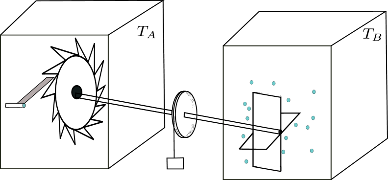
Figure 1: Schematic illustration of the Feynman’s ratchet.

The discrete model of Feynman’s ratchet proposed by Jarzynski and Mazonka can be envisaged as a particle hopping between neighboring sites on a 1D regular lattice. As shown in Fig. 2, the potential energy of each site $i$ has two modes $m=1,2$.

$$U_{i}^{(m)}=\begin{cases}-ifd\text{,}&m=1\text{,}\\ \alpha\cdot\left[(i\;\text{mod}\;3)-1\right]-ifd\text{,}&m=2\text{.}\end{cases}$$ (1)

Here, $f$ denotes the load, $\alpha$ is the energy unit and $d$ is the lattice spacing. Due to periodicity, we only need to consider one tooth on the ratchet: the system consists of six possible states, $n=1,\cdots,6$. The energies are listed in Table 1. Only those transitions between neighboring sites in the same mode and those between modes on the same site are allowed.

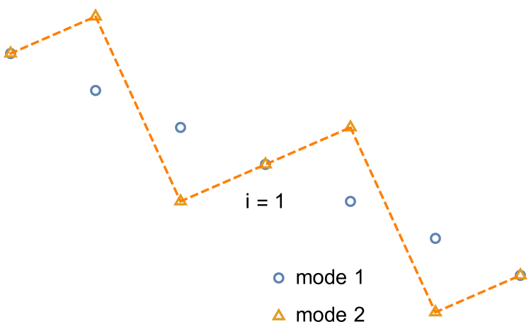
Figure 2: The landscape of potential energy $U_{i}^{(m)}$ for two modes, $m=1,2$, in the presence of an external load $f=\alpha/2d$. Alternatively, we denote the potential energy as $U_{n},n=1,\cdots,6.$ See Table 1 for one to one correspondance.

Table 1: The energies of the six states.

state $n$	mode $m$	site $i$	potential energy $U_{n}$
1	1	0	$0$
2	1	1	$-fd$
3	1	2	$-2fd$
4	2	0	$-\alpha$
5	2	1	$-fd$
6	2	2	$\alpha-2fd$

We now denote by ${\cal P}_{n}(t)$ the probability of finding the system in state $n$ at time $t$. Its evolution is governed by the master equation

$$\frac{\rm d}{{\rm d}t}{\cal P}_{n}(t)=\sum_{n^{\prime}(\neq n)}\Big{[}W_{nn^{\prime}}{\cal P}_{n^{\prime}}(t)-W_{n^{\prime}n}{\cal P}_{n}(t)\Big{]}\text{.}$$ (2)

Transiton rates are given by 

$$W_{nn^{\prime}}=\frac{\beta\Delta U_{n\leftarrow n^{\prime}}}{\exp(\beta\Delta U_{n\leftarrow n^{\prime}})-1}$$ (3)

for allowed transitions and $W_{nn^{\prime}}=0$ for forbidden ones. Here $\Delta U_{n\leftarrow n^{\prime}}$ is the potential energy change associated with the transition from state $n^{\prime}$ to $n$. For transition $n^{\prime}\to n$ within one period,the energy difference is $\Delta U_{n\leftarrow n^{\prime}}=U_{n}-U_{n^{\prime}}$ with energies $U_{n}$ listed in Table 1. However, for those transitions across the boundaries, the potential energy changes are given by

$$\Delta U_{3\leftarrow 1}=fd\text{,}$$ (4)

$$\Delta U_{1\leftarrow 3}=-fd\text{,}$$ (5)

$$\Delta U_{6\leftarrow 4}=2\alpha+fd\text{,}$$ (6)

$$\Delta U_{4\leftarrow 6}=-2\alpha-fd\text{.}$$ (7)

$\beta\equiv 1/(k_{\rm B}T)$ is the inverse temperature and $k_{\rm B}$ is Boltzmann’s constant. Depending on the the type of transition, $T$ may take different values: $T=T_{A}$ for switches between two modes and $T=T_{B}$ for jumps between neighbouring sites. The rate function (3) satisfies the detailed balance condition

$$W_{nn^{\prime}}=W_{n^{\prime}n}\exp(-\beta\Delta U_{n\leftarrow n^{\prime}})$$ (8)

originating from the microscopic reversibility.

The master equation (2) with explicit transition rates can be simulated with the Gillespie’s algorithm  Gillespie (1976), which is an explicit method to generate random trajectories for Markov stochastic processes. If we define the diagonal elements to be

$$W_{nn}\equiv-\sum_{n^{\prime}(\neq n)}W_{n^{\prime}n}\text{,}$$ (9)

the master equation (2) can be rewritten into a matrix form as

$$\frac{\rm d}{{\rm d}t}{\boldsymbol{\cal P}}={\boldsymbol{\sf L}}\cdot{\boldsymbol{\cal P}}\text{,}$$ (10)

where ${\boldsymbol{\cal P}}=({\cal P}_{1},\cdots,{\cal P}_{6})^{\rm T}$ and ${\boldsymbol{\sf L}}=[W_{nn^{\prime}}]$. Each column of ${\boldsymbol{\sf L}}$ sums to zero so that it guarantees the conservation of probability.

III The Currents and Their Corresponding Affinities

Intuitively we can infer that there are two coupled currents in the ratchet and pawl system, namely the energy flow between two heat baths and the displacement of the load. When the system switches the mode, reservoir $A$ exchanges an energy $\alpha$ with the system. Therefore the instantaneous energy current from reservoir A to the system is defined as

$$j_{E}(t)\equiv\alpha\sum_{k=1}^{+\infty}\Big{[} \delta\left(t-t_{k}^{1\leftarrow 4}\right)-\delta\left(t-t_{k}^{4\leftarrow 1}\right)$$

$$+\delta\left(t-t_{k}^{6\leftarrow 3}\right)-\delta\left(t-t_{k}^{3\leftarrow 6}\right)\Big{]}\text{,}$$ (11)

where $t_{k}^{n^{\prime}\leftarrow n}$ is the $k$-th random transition from state $n$ to $n^{\prime}$. Similarly, the instantaneous current of displacement (velocity) of the load is defined by considering transitions between neighboring sites in both modes, yielding

$$j_{X}(t)\equiv d\sum_{k=1}^{+\infty}\Big{[} \delta\left(t-t_{k}^{2\leftarrow 1}\right)-\delta\left(t-t_{k}^{1\leftarrow 2}\right)+\delta\left(t-t_{k}^{3\leftarrow 2}\right)-\delta\left(t-t_{k}^{2\leftarrow 3}\right)+\delta\left(t-t_{k}^{1\leftarrow 3}\right)-\delta\left(t-t_{k}^{3\leftarrow 1}\right)$$

$$+\delta\left(t-t_{k}^{5\leftarrow 4}\right)-\delta\left(t-t_{k}^{4\leftarrow 5}\right)+\delta\left(t-t_{k}^{6\leftarrow 5}\right)-\delta\left(t-t_{k}^{5\leftarrow 6}\right)+\delta\left(t-t_{k}^{4\leftarrow 6}\right)-\delta\left(t-t_{k}^{6\leftarrow 4}\right)\Big{]}\text{.}$$ (12)

Correspondingly, there are two driving forces or affinities, which can be determined by analyzing the master equation (2) with Schnakenberg’s network theory Schnakenberg (1976); Faggionato and Pietro (2011). In this theory, a graph is associated with the Markov jump process. Vertices represent the states while the edges stand for the allowed transitions between states. The graph for the ratchet system is depicted in Fig. 3. From the so-constructed graph, the affinities can be calculated from the transition rates along cyclic paths and their reversals. For example, the cyclic path associated with energy $\alpha$ transferred from reservoir A to B and its reversed path could be

$${\cal C}_{E}:1\to 2\to 5\to 4\to 1\text{,}$$ (13)

$${\cal C}_{E}^{r}:1\to 4\to 5\to 2\to 1\text{,}$$ (14)

and the affinity is given by

$$A_{E}=\frac{1}{\alpha}\ln\frac{W_{14}W_{45}W_{52}W_{21}}{W_{12}W_{25}W_{54}W_{41}}=\beta_{B}-\beta_{A}\text{.}$$ (15)

The prefactor is aimed to set the affinity in the unit of energy. Similarly, for a load displacement of $3d$, the cyclic path and its reversal could be

$${\cal C}_{X}:1\to 2\to 3\to 1\text{,}$$ (16)

$${\cal C}_{X}^{r}:1\to 3\to 2\to 1\text{.}$$ (17)

The corresponding affinity is

$$A_{X}=\frac{1}{3d}\ln\frac{W_{13}W_{32}W_{21}}{W_{12}W_{23}W_{31}}=f\beta_{B}\text{.}$$ (18)

We notice that although the transition rates usually depend on the states, the so-obtained affinities only depend on the thermodynamic forces which are of physical importance. Since the graph only contains six vertices, it can be easily decomposed into four independent cycles which form the fundamental set. Detailed analysis is presented in Appendix A.

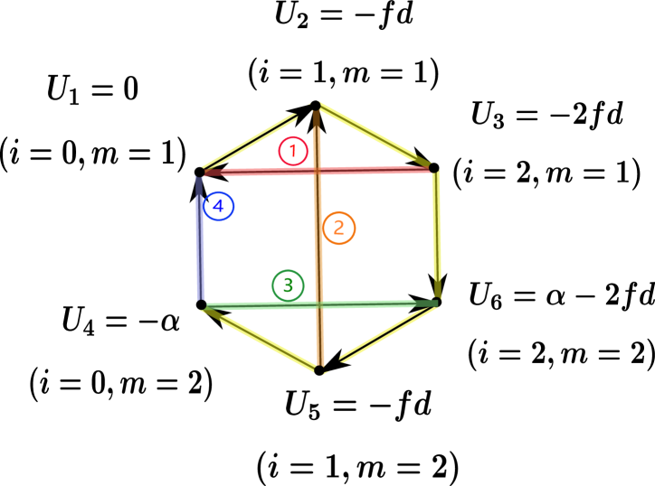
Figure 3: The graph of the discrete model with vertices representing the distinct states, edges denoting the allowed transitions. The subgraph consisting of the thick yellow lines is chosen as the maximal tree. The corresponding chords are numbered with ①, ②, ③, ④.

IV Fluctuation Theorem for the Currents

IV.1 Full Counting Statistics

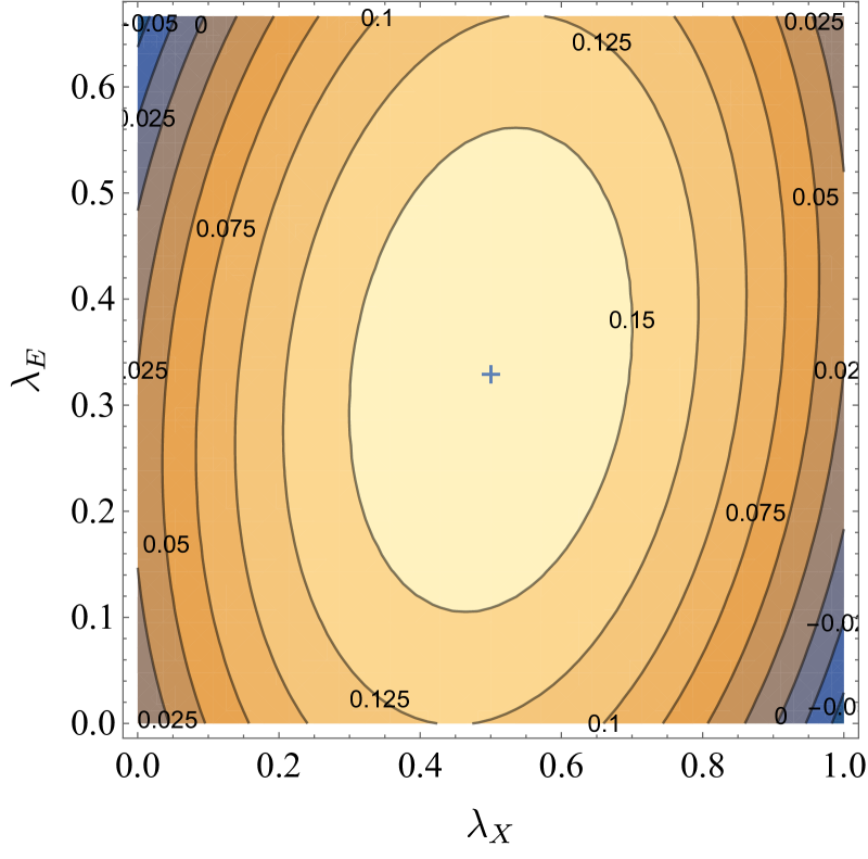
Figure 4: The contour map of the cumulant generating function $Q(\lambda_{X},\lambda_{E})$ centering at $(A_{X}/2=1/2,A_{E}/2=1/3)$ with $T_{A}=3,T_{B}=1,f=1$.

Giving access to all cumulants of the current, full counting statistics is a powerful theoretical method to study fluctuations. In order to investigate the full counting statistics, we first define the accumulated energy flowing across the ratchet system and the accumulated displacement of the load over the time interval $[0,\;t]$

$$E(t)\equiv\int_{0}^{t}j_{E}(t^{\prime})\,{\rm d}t^{\prime}\text{,}\hskip 14.22636ptX(t)\equiv\int_{0}^{t}j_{X}(t^{\prime})\,{\rm d}t^{\prime}\text{.}$$ (19)

Then it is eay to obtain the extended master equation for the joint probability ${\cal P}_{n}(E,X,t)$ of finding the system in state $n$ at time $t$ while having absorbed energy $E$ from reservoir A and moved by a distance $X$ (see Appendix B ). By summing over all states, we can also define the marginal probability ${\cal P}(E,X,t)\equiv\sum_{n}{\cal P}_{n}(E,X,t)$. Note that the energy and displacement take discrete values and change according to $E\to E\pm\alpha$ and $X\to X\pm d$. We further define the cumulant generating function as

$$Q(\lambda_{E},\lambda_{X})\equiv\lim_{t\to\infty}-\frac{1}{t}\ln\sum_{E,X}{\cal P}(E,X,t)\,{\rm e}^{-\lambda_{E}E-\lambda_{X}X}\text{,}$$ (20)

where $\lambda_{E}$ and $\lambda_{X}$ are the counting parameters. The cumulant generating function (CGF) $Q(\lambda_{E},\lambda_{X})$ can be obtained by solving for the leading eigenvalue of operator ${\boldsymbol{\sf L}}_{\lambda_{E},\lambda_{X}}$

$${\boldsymbol{\sf L}}_{\lambda_{E},\lambda_{X}}\cdot{\boldsymbol{\Psi}}_{\lambda_{E},\lambda_{X}}=-Q(\lambda_{E},\lambda_{X}){\boldsymbol{\Psi}}_{\lambda_{E},\lambda_{X}}\text{,}$$ (21)

with ${\boldsymbol{\sf L}}_{\lambda_{E},\lambda_{X}}$ being

$${\boldsymbol{\sf L}}_{\lambda_{E},\lambda_{X}}\equiv\begin{pmatrix}W_{11}&W_{12}\,{\rm e}^{d\lambda_{X}}&W_{13}\,{\rm e}^{-d\lambda_{X}}&W_{14}\,{\rm e}^{-\alpha\lambda_{E}}&W_{15}&W_{16}\bigstrut\\ W_{21}\,{\rm e}^{-d\lambda_{X}}&W_{22}&W_{23}\,{\rm e}^{d\lambda_{X}}&W_{24}&W_{25}&W_{26}\bigstrut\\ W_{31}\,{\rm e}^{d\lambda_{X}}&W_{32}\,{\rm e}^{-d\lambda_{X}}&W_{33}&W_{34}&W_{35}&W_{36}\,{\rm e}^{\alpha\lambda_{E}}\bigstrut\\ W_{41}\,{\rm e}^{\alpha\lambda_{E}}&W_{42}&W_{43}&W_{44}&W_{45}\,{\rm e}^{d\lambda_{X}}&W_{46}\,{\rm e}^{-d\lambda_{X}}\bigstrut\\ W_{51}&W_{52}&W_{53}&W_{54}\,{\rm e}^{-d\lambda_{X}}&W_{55}&W_{56}\,{\rm e}^{d\lambda_{X}}\bigstrut\\ W_{61}&W_{62}&W_{63}\,{\rm e}^{-\alpha\lambda_{E}}&W_{64}\,{\rm e}^{d\lambda_{X}}&W_{65}\,{\rm e}^{-d\lambda_{X}}&W_{66}\bigstrut\end{pmatrix}\text{.}$$ (22)

Since the matrix exponential $\exp({\boldsymbol{\sf L}}_{\lambda_{E},\lambda_{X}}t)>0$, the Perron-Frobenius theorem applies and the leading eigenvalue $-Q(\lambda_{E},\lambda_{X})$ of ${\boldsymbol{\sf L}}_{\lambda_{E},\lambda_{X}}$ corresponds to the real maximum eigenvalue $\exp[-Q(\lambda_{E},\lambda_{X})]$ of $\exp({\boldsymbol{\sf L}}_{\lambda_{E},\lambda_{X}}t)$ in magnitude ($t>0$). So the ${\boldsymbol{\Psi}}_{\lambda_{E},\lambda_{X}}$ can be asymptotically evaluated as

$${\boldsymbol{\Psi}}_{\lambda_{E},\lambda_{X}}\sim_{t\to\infty}\sf exp\left({\boldsymbol{\sf L}}_{\lambda_{E},\lambda_{X}}t\right)\cdot{\boldsymbol{\psi}}\text{,}$$ (23)

which is then normalized

$${\boldsymbol{\Psi}}_{\lambda_{E},\lambda_{X}}\leftarrow\frac{{\boldsymbol{\Psi}}_{\lambda_{E},\lambda_{X}}}{\sqrt{{\boldsymbol{\Psi}}_{\lambda_{E},\lambda_{X}}^{\rm T}\cdot{\boldsymbol{\Psi}}_{\lambda_{E},\lambda_{X}}}}\text{.}$$ (24)

Here ${\boldsymbol{\Psi}}_{\lambda_{E},\lambda_{X}}$ is the eigenvector corresponding to the leading eigenvalue of ${\boldsymbol{\sf L}}_{\lambda_{E},\lambda_{X}}$, and $\boldsymbol{\psi}$ is the randomly chosen distribution supposed to include the desired component. The matrix exponential can be computed using Padé approximation  Higham (2008). The cumulant generating function is calculated as

$$Q(\lambda_{E},\lambda_{X})=-{\boldsymbol{\Psi}}_{\lambda_{E},\lambda_{X}}^{\rm T}\cdot{\boldsymbol{\sf L}}_{\lambda_{E},\lambda_{X}}\cdot{\boldsymbol{\Psi}}_{\lambda_{E},\lambda_{X}}\text{.}$$ (25)

The stationary distribution is given by ${\boldsymbol{\cal P}}_{\rm st}={\boldsymbol{\Psi}}_{0,0}$. Fig. 4 shows in contour map the cumulant generating function in the plane of the counting parameters $\lambda_{E}$ and $\lambda_{X}$. Two cross sections are plotted in Fig. 5.

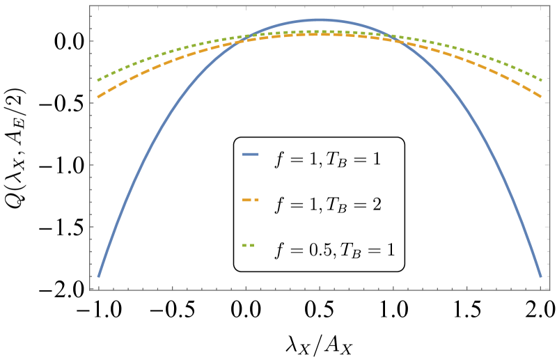
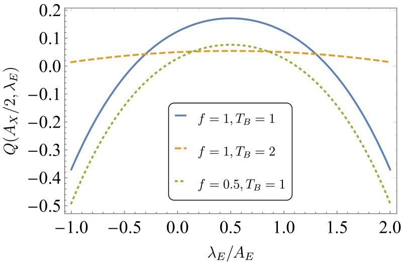
Figure 5: The cross sections of the cumulant generating function $Q(\lambda_{X},\lambda_{E})$. In the left panel, the counting parameter is $\lambda_{E}=A_{E}/2$ while in the right panel $\lambda_{X}=A_{X}/2$. In both panels, $T_{A}=3$.

IV.2 Fluctuation Theorem

We find that matrix ${\boldsymbol{\sf L}}_{\lambda_{E},\lambda_{X}}$ (22) exhibits the symmetry relation

$${\boldsymbol{\sf M}}^{-1}\cdot{\boldsymbol{\sf L}}_{\lambda_{E},\lambda_{X}}\cdot{\boldsymbol{\sf M}}={\boldsymbol{\sf L}}_{A_{E}-\lambda_{E},A_{X}-\lambda_{X}}^{\rm T}$$ (26)

under similarity transformation with matrix ${\boldsymbol{\sf M}}$ Lau et al. (2007); Lacoste and Mallick (2009); Lacoste et al. (2008)

$${\boldsymbol{\sf M}}=\begin{pmatrix}1&0&0&0&0&0\bigstrut\\ 0&1&0&0&0&0\bigstrut\\ 0&0&1&0&0&0\bigstrut\\ 0&0&0&{\rm e}^{\alpha/{dT_{B}}}&0&0\bigstrut\\ 0&0&0&0&1&0\bigstrut\\ 0&0&0&0&0&{\rm e}^{-\alpha/{dT_{B}}}\bigstrut\\ \end{pmatrix}\text{.}$$ (27)

As similarity transformation of the matrix does not change the eigenvalues, the relation (26) implies

$$Q({\lambda_{E},\lambda_{X}})=Q(A_{E}-\lambda_{E},A_{X}-\lambda_{X})\text{,}$$ (28)

which is known as Gallavotti-Cohen symmetry Gallavotti and Cohen (1995a, a); Faggionato and Pietro (2011). This symmetry for the CGF can be seen in Fig. 4 and Fig. 5. The CGF is directly related to the large deviation function through Legendre-Fenchel transform Touchette (2009)

$$I(e,x)=\max_{\lambda_{E},\lambda_{X}}\Big{[}Q(\lambda_{E},\lambda_{X})-\left(\lambda_{E}e+\lambda_{X}x\right)\Big{]}\text{.}$$ (29)

$I(e,x)$ is the large deviation rate function of the probability ${\cal P}(E=et,X=xt,t)$ defined as follows

$${\cal P}(E=et,X=xt,t)\sim_{t\to\infty}{\rm e}^{-tI(e,x)}\text{.}$$ (30)

The Gallavotti-Cohen symmetry relation (28) immediately implies

$$I(-e,-x)-I(e,x)=A_{E}e+A_{X}x\text{,}$$ (31)

leading all the way to

$$\frac{{\cal P}(E,X,t)}{{\cal P}(-E,-X,t)}\simeq_{t\to\infty}{\rm e}^{A_{E}E+A_{X}X}\text{,}$$ (32)

which is the usual form of fluctuation theorem. This relation can also be derived based on the cycle theory (See Appendix. A).

What’s more, the similarity between ${\boldsymbol{\sf L}}_{\lambda_{E},\lambda_{X}}$ and ${\boldsymbol{\sf L}}_{A_{E}-\lambda_{E},A_{X}-\lambda_{X}}^{\rm T}$ implies that all eigenvalues are the same, leading to a finite-time fluctuation theorem

$$\left\langle{\rm e}^{-\lambda_{E}E-\lambda_{X}X}\right\rangle=\left\langle{\rm e}^{-(A_{E}-\lambda_{E})E-(A_{X}-\lambda_{X})X}\right\rangle\text{.}$$ (33)

This coincides with the fluctuation theorem of entropy production Seifert (2005).

IV.3 Thermodynamic Entropy Production

For the ratchet system in nonequilibrium steady state, the mean currents of energy and displacement can be evaluated as

$$J_{E}=\lim_{t\to\infty}\frac{1}{t}\sum_{E,X}{\cal P}(E,X,t)E\text{,}$$ (34)

$$J_{X}=\lim_{t\to\infty}\frac{1}{t}\sum_{E,X}{\cal P}(E,X,t)X\text{.}$$ (35)

The thermodynamic entropy production rate Prigogine and Rysselberghe (1963); Callen and Scott (1998) in units of Boltzmann’s constant is identified as the sum of products of the affinities and the corresponding mean currents. According to the fluctuation theorem (32), it can be expressed as

$$\frac{1}{k_{\rm B}}\frac{{\rm d}_{\rm i}S}{{\rm d}t} =A_{E}J_{E}+A_{X}J_{X}$$

$$=\lim_{t\to\infty}\frac{1}{t}\sum_{E,X}{\cal P}(E,X,t)\ln\frac{{\cal P}(E,X,t)}{{\cal P}(-E,-X,t)}\text{,}$$ (36)

in terms of the Kullback-Leibler divergence of ${\cal P}(E,X,t)$ and ${\cal P}(-E,-X,t)$. The term on the r.h.s. of Eq. (36) is always non-negative, which is in accordance with the second law of thermodynamics. Also, Eqs. (32,33) indicate that there is a nonzero probability of observing the "violation" of the second law in the Feynman’s ratchet, i.e.,$A_{E}E+A_{X}X<0$. But in the Feynman’s ratchet, the probability of observing such a "violation" becomes negligibly small in the long time limit since both $E$ and $X$ are proportional to $t$. These results obviously agree with our intuition about Feynman’s ratchet.

V Symmetry Relations for the Response Coefficients

It has been shown in Refs. Andrieux et al. (2009); Barbier and Gaspard (2018, 2020a, 2020b); Gu and Gaspard (2020, 2019); Derrida (2007); Gao and Limmer (2019) that the Gallavotti-Cohen symmetry relation provides a unified framework from which one can derive relations between response coefficients to an arbitrary order (See Eqs. (42-44) below). In previous sections we fix the affinities $A_{X},A_{E}$. In this section, we will evaluate the response properties for different values of afffinites. Hence, the CGF $Q(\lambda_{X},\lambda_{E})$ should be rewrittened as $Q(\boldsymbol{\lambda},\bf A)$. Here $\boldsymbol{\lambda}=\set{\lambda_{1},\lambda_{2}},\bf A$$=\left\{A_{1},A_{2}\right\}$, $1=X,2=E.$ The cumulants can be evaluated by taking successive derivatives of the CGF with respect to the counting parameters. The average currents and diffusivities are given by

$$J_{i}({\bf A})=\left.\frac{\partial Q({\boldsymbol{\lambda}};{\bf A})}{\partial\lambda_{i}}\right|_{{\boldsymbol{\lambda}}={\bf 0}}\text{,}$$ (37)

$$D_{ij}({\bf A})=\left.-\frac{1}{2}\frac{\partial^{2}Q({\boldsymbol{\lambda}};{\bf A})}{\partial\lambda_{i}\partial\lambda_{j}}\right|_{{\boldsymbol{\lambda}}={\bf 0}}\text{.}$$ (38)

In the mean time, we can expand the mean currents in the power series of afffinites as

$$J_{i}({\bf A})=\sum_{j}L_{i,j}A_{j}+\frac{1}{2}\sum_{j,k}M_{i,jk}A_{j}A_{k}+\cdots$$ (39)

in terms of the linear and nonlinear response coefficients defined by Andrieux et al. (2009)

$$L_{i,j}\equiv\left.\frac{\partial^{2}Q({\boldsymbol{\lambda}};{\bf A})}{\partial\lambda_{i}\partial A_{j}}\right|_{{\boldsymbol{\lambda}}={\bf A}={\bf 0}}\text{,}$$ (40)

$$M_{i,jk}\equiv\left.\frac{\partial^{3}Q({\boldsymbol{\lambda}};{\bf A})}{\partial\lambda_{i}\partial A_{j}\partial A_{k}}\right|_{{\boldsymbol{\lambda}}={\bf A}={\bf 0}}\text{,}$$ (41)

where we notice $M_{i,jk}=M_{i,kj}$ by definition. From the Gallavotti-Cohen symmetry relation (28), we can easily deduce the fluctuation-dissipation theorem Kubo (1966)

$$L_{i,j}=D_{ij}({\bf A=\bf 0})\text{,}$$ (42)

and Onsager reciprocal relations Onsager (1931); Casimir (1945); Andrieux et al. (2009); Jarzynski and Mazonka (1999)

$$L_{i,j}=L_{j,i}\text{.}$$ (43)

We can also prove the relations characterizing the second order response properties Andrieux et al. (2009)

$$M_{i,jk}=R_{ij,k}+R_{ik,j}\text{,}$$ (44)

where $R_{ij,k}$ is defined as the linear response coefficient of the diffusivity around equilibrium,

$$R_{ij,k}\equiv\left.\frac{\partial D_{ij}}{\partial A_{k}}\right|_{{\bf A}={\bf 0}}=-\frac{1}{2}\left.\frac{\partial^{3}Q({\boldsymbol{\lambda}};{\bf A})}{\partial\lambda_{i}\partial\lambda_{j}\partial A_{k}}\right|_{{\boldsymbol{\lambda}}={\bf A}={\bf 0}}\text{.}$$ (45)

We notice that Onsager reciprocal relation (43) is the direct consequence of the fluctuation-dissipation relations (42) together with the symmetry of the diffusivities $D_{ij}=D_{ji}$. Higher order relations can be obtained likewise.

We do a numerical test of the relations (42)-(44) in the ratchet system. For this purpose, we first calculate the CGF $Q(\lambda_{X},\lambda_{E};A_{X},A_{E})$ for several points around $\lambda_{X}=\lambda_{E}=A_{X}=A_{E}=0$. Then we perform the Lagrange interpolation to obtain the multivariate polynomial approximating the CGF. Finally, the values of $L_{i,j}$, $D_{ij}$, $M_{i,jk}$ and $R_{ij,k}$ for $i,j,k=1,2$ $(1$ for $X,2$ for $E)$ are calculated by taking derivatives according to their definitions. The agreement between the related quantities is clearly demonstrated in Figs. 6 and 7. Thus for the ratchet system, the validity of predictions of fluctuation theorems is tested in both linear and nonlinear regimes.

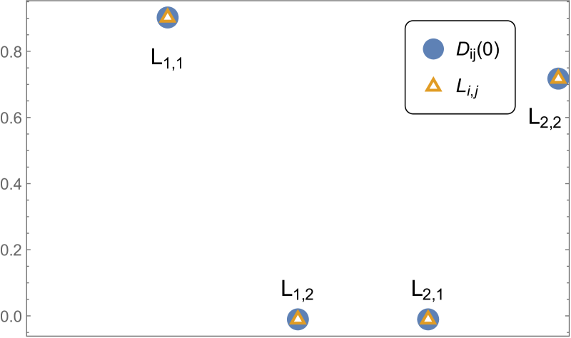
Figure 6: The comparison between linear response coefficients $L_{i,j}$ (orange triangles) and diffusivities in equilibrium $D_{ij}({\bf 0})$ (blue circles). The parameters are taken to be the same as those in Fig. 4.

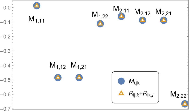
Figure 7: The comparison between the second-order response coefficients $M_{i,jk}$ and $R_{i,jk}+R_{i,kj}$, where $R_{i,jk}$ is defined by Eq. (45). Same parameters as in Fig. 4.

VI Conclusion and Perspectives

In this article, we investigate the full counting statistics of Feynman’s ratchet and show that Gallavotti-Cohen fluctuation theorem holds for the currents in the discrete model of Feynman’s ratchet. The Markovian stochastic jump process is described by the master equation, with transition rates determined by energy difference. Detailed balance condition is guaranteed so that the dynamics is compatible with the underlying law of microreversibility. Feynman’s ratchet and pawl system is driven out of equilibrium by the temperature difference between two heat baths and also by the external load. Correspondingly, there are two physical currents coupled to each other. By perfoming full counting statistics analysis of the currents, we obtain the CGF which manifests a symmetry relation. This symmetry quantitatively characterizes the fluctuation and the probablistic "violation" of the second law by the Feynman’s ratchet and hence deepens our understanding about fluctuating properties of the famous model from the qualitative way to the quantitative way. In addition, we point out that the currents exhibit linear and nonlinear response properties in the ratchet system, as predicted by the fluctuation theorem. We numerically verify the relation between the linear response coefficients and the equilibrium diffusivities. Further we verify in detail that the second-order response coefficients are related to the linear response of the diffusivities. Higher order relations can be obtained likewise.

As the six-state model of Feynman’s ratchet is simple enough, it can be regarded as a basis for studying more sophisticated systems, e.g., spatially extended models. Considering that the pawl stochastically switches between two modes, a feedback control can be applied to determine whether or not the external load is to be attached. In this way, a fluctuation theorem involving information flow could possibly be explored.

Appendix A Cycle Decomposition

Schnakenberg found that Schnakenberg (1976) stochastic processes described by the master equation can be investigated by carrying out graph analysis and that the nonequilibrium constraints exerted on a system are related to affinities of the cycles in the graph. This mathematical tool is applied here to study fluctutaion theorem for the currents – energy flow and load displacement.

In the basic graph $G$, the vertices represent the distinct states while the edges stand for the allowed transitions between states. Then we choose a maximal tree $T(G)$ which is a covering subgraph of $G$. The requirements for a maximal tree are listed as follows:

• $T(G)$ covers all the vertices of $G$ and all the edges of $T(G)$ belong to $G$;

• $T(G)$ must be connected;

• $T(G)$ contains no circuit.

The edges $l$ of graph $G$ that does not belong to $T(G)$ are refered to as chords of maximal tree $T(G)$. By respectively adding one chord to the maximal tree, we get exactly one closed circuit at a time in the resulting subgraph $T(G)+l$. The set of circuits is called a fundamental set $\{C_{l}\}$. As marked in Fig. 3, by choosing the maximal tree $T(G)$ in yellow, the remaining four edges automatically become its chords. It has been identified that there are four independent cycles in the fundamental set $\{C_{l}\}=\{C_{\rm I},\,C_{\rm II},\,C_{\rm III},\,C_{\rm IV}\}$

$$C_{\rm I}=\left(e_{1\to 2},\,e_{2\to 3},\,e_{3\to 1}\right)\text{,}$$ (46)

$$C_{\rm II}=\left(e_{2\to 3},\,e_{3\to 6},\,e_{6\to 5},\,e_{5\to 2}\right)\text{,}$$ (47)

$$C_{\rm III}=\left(e_{4\to 6},\,e_{6\to 5},\,e_{5\to 4}\right)\text{,}$$ (48)

$$C_{\rm IV}=\left(e_{1\to 2},\,e_{2\to 3},\,e_{3\to 6},\,e_{6\to 5},\,e_{5\to 4},\,e_{4\to 1}\right)\text{,}$$ (49)

where $e_{i\to j}$ denotes the directional edge representing the transition from state $i$ to $j$. Schnakenberg’s graph analysis tells us that each cycle $C$ in the basic graph can be expressed as linear combination of cycles in the fundamental set. In the long-time limit, the initial state becomes irrelevant and the whole trajectory forms a closed cycle $C(t)$. So we have

$$C(t)=a_{\rm I}(t)C_{\rm I}+a_{\rm II}(t)C_{\rm II}+a_{\rm III}(t)C_{\rm III}+a_{\rm IV}(t)C_{\rm IV}\text{.}$$ (50)

Now we apply Schnakenberg’s network theory to prove that Gallavotti-Cohen symmetry exists in the CGF of the energy flow and load displacement. The load displacement can be evaluated by counting the jump times between states in both modes

$$X(t)=d\Big{[} S_{1\to 2}+S_{2\to 3}+S_{3\to 1}$$

$$\quad\quad+S_{4\to 5}+S_{5\to 6}+S_{6\to 1}\Big{]}C(t)\text{,}$$ (51)

where the operator $S_{i\to j}$ counts the jump times across the edge $e_{i\to j}$. Such linear operators $S_{i\to j}$ separately act on independent cycles

$$S_{1\to 2}C(t)=a_{\rm I}(t)+a_{\rm IV}(t)\text{,}$$ (52)

$$S_{2\to 3}C(t)=a_{\rm I}(t)+a_{\rm II}(t)+a_{\rm IV}(t)\text{,}$$ (53)

$$S_{3\to 1}C(t)=a_{\rm I}(t)\text{,}$$ (54)

$$S_{4\to 5}C(t)=-a_{\rm III}(t)-a_{\rm IV}(t)\text{,}$$ (55)

$$S_{5\to 6}C(t)=-a_{\rm II}(t)-a_{\rm III}(t)-a_{\rm IV}(t)\text{,}$$ (56)

$$S_{6\to 4}C(t)=-a_{\rm III}(t)\text{.}$$ (57)

Substituding (52-57) into (51) we have

$$X(t)=d\Big{[}3a_{\rm I}(t)-3a_{\rm III}(t)\Big{]}\text{.}$$ (58)

The energy transferred from the reservoir $A$ to the system can be similarly evaluated by considering only the transitions between two modes

$$E(t)=\alpha\Big{[}S_{4\to 1}+S_{3\to 6}\Big{]}C(t)=\alpha\Big{[}a_{\rm II}(t)+2a_{\rm IV}(t)\Big{]}\text{.}$$ (59)

The CGF for the energy flow and load displacement can be written as

$$Q(\lambda_{E},\lambda_{X}) =\underset{t\rightarrow\infty}{\lim}-\frac{1}{t}\ln\left\langle{\rm e}^{-\lambda_{E}E(t)-\lambda_{X}X(t)}\right\rangle$$

$$=\lim_{t\to\infty}-\frac{1}{t}\ln\left\langle{\rm e}^{-3\lambda_{X}a_{\rm I}(t)-\lambda_{E}a_{\rm II}(t)+3\lambda_{X}a_{\rm III}(t)-2\lambda_{E}a_{\rm IV}(t)}\right\rangle\text{.}$$ (60)

Recalling the fluctuation theorem for the currents crossing the chords proved by Andrieux and Gaspard Andrieux and Gaspard (2007a), the CGF of independent currents along the chords

$$q(\{\lambda_{l}\})=\lim_{t\to\infty}-\frac{1}{t}\ln\left\langle{\rm e}^{\sum_{l}\lambda_{l}a_{l}(t)}\right\rangle$$ (61)

exhibits the following symmetry

$$q(\{\lambda_{l}\})=q(\{A_{l}-\lambda_{l}\})\text{,}$$ (62)

where $A_{l}$ is the affinity of the independent cycle in the fundamental set and the notation $\{\lambda_{l}\}$ is short for $\{\lambda_{\rm I},\cdots,\lambda_{\rm IV}\}$. In this case, the affinities $\{A_{l}\}$ can be calculated by taking the log of ratio of transition rate products in both directions

$$A_{\rm I}=\frac{1}{d}\ln\frac{W_{13}W_{32}W_{21}}{W_{12}W_{23}W_{31}}=3f\beta_{B}\text{,}$$ (63)

and similarly

$$A_{\rm II}=\beta_{B}-\beta_{A}\text{,}$$ (64)

$$A_{\rm III}=-3f\beta_{B}\text{,}$$ (65)

$$A_{\rm IV}=2\left(\beta_{B}-\beta_{A}\right)\text{.}$$ (66)

When $\{C_{l}\}$ is a fundamental set, the coefficients $\{a_{l}(t)\}$ in cycle decomposition equal the integrated current along the chords, i.e., the number of times crossing each chord. Then the CGF for joint energy and displacement flow $Q(\lambda_{E},\lambda_{X})$ can be mapped onto $q(\{\lambda_{l}\})$ as

$$Q(\lambda_{E},\lambda_{X}) =q\left(3\lambda_{X},\lambda_{E},-3\lambda_{X},2\lambda_{E}\right)$$

$$=q\left(A_{\rm I}-3\lambda_{X},A_{\rm II}-\lambda_{E},A_{\rm III}+3\lambda_{X},A_{\rm IV}-2\lambda_{E}\right)$$

$$=q\left(3f\beta_{B}-3\lambda_{X},\beta_{B}-\beta_{A}-\lambda_{E},-3f\beta_{B}+3\lambda_{X},2\beta_{B}-2\beta_{A}-2\lambda_{E}\right)$$

$$=Q(A_{E}-\lambda_{E},A_{X}-\lambda_{X})\text{,}$$ (67)

which gives the Gallavotti-Cohen symmetry (28).

Appendix B Derivation of Eq. (22)

The generating function for the joint energy flow (from reservoir A to the system) and the displacement is defined as

$$\boldsymbol{\Psi}_{\lambda_{E},\lambda_{X}}(t)=\underset{n}{\sum}(\boldsymbol{\Psi}_{\lambda_{E},\lambda_{X}})_{n}(t)\text{,}$$ (68)

$$(\boldsymbol{\Psi}_{\lambda_{E},\lambda_{X}})_{n}(t) =\int\mathrm{d}E\mathrm{d}X\mathrm{e}^{-\lambda_{E}E-\lambda_{X}X}{\cal P}_{n}(E,X,t),$$ (69)

where ${\cal P}_{n}(E,X,t)$ represents the probability of finding the system in state $n$ at time $t$ while having absorbed energy $E(t)$ from reservoir A and moved by a displacement $X(t)$. The displacement of the particle and the heat absorbed from reservoir A during a transition from state $m$ to state $n$ is given by $\Delta X_{nm}$ and $\Delta E_{nm}$.

In a small time interval $\tau$ the variation of ${\cal P}_{n}(E,X,t)$ is given by

$${\cal P}_{n}(E,X,t+\tau) \approx{\cal P}_{n}(E,X,t)+\tau\underset{m(\neq n)}{\sum}\Bigl{[}W_{nm}{\cal P}_{m}(E-\Delta E_{nm},X-\Delta X_{nm},t)-W_{mn}{\cal P}_{n}(E,X,t)\Bigr{]}$$ (70)

$$={\cal P}_{n}(E,X,t)+\tau\underset{m(\neq n)}{\sum}\biggl{\{}W_{nm}\underset{k,l=0}{\sum}\Bigl{[}\frac{(-\Delta E_{nm})^{k}}{k!}\frac{(-\Delta X_{nm})^{l}}{l!}\frac{\partial^{k+l}{\cal P}_{m}(E,X,t)}{\partial E^{k}\partial X^{l}}\Bigr{]}-W_{mn}{\cal P}_{n}(E,X,t)\biggr{\}}.$$ (71)

The joint distribution function ${\cal P}_{n}(E,X,t)$ evolves as

$$\frac{\partial{\cal P}_{n}(E,X,t)}{\partial t}=\underset{m(\neq n)}{\sum}\biggl{\{}W_{nm}\underset{k,l}{\sum}\Bigl{[}\frac{(-\Delta E_{nm})^{k}}{k!}\frac{(-\Delta X_{nm})^{l}}{l!}\frac{\partial^{k+l}{\cal P}_{m}(E,X,t)}{\partial E^{k}\partial X^{l}}\Bigr{]}-W_{mn}{\cal P}_{n}(E,X,t)\biggr{\}}$$ (72)

with $(\Delta E)_{nm}$ and $(\Delta X)_{nm}$ respectively given by

$$(\Delta X)_{nm}=d\left(\begin{array}[]{cccccc}0&-1&1&0&0&0\\ 1&0&-1&0&0&0\\ -1&1&0&0&0&0\\ 0&0&0&0&-1&1\\ 0&0&0&1&0&-1\\ 0&0&0&-1&1&0\end{array}\right)\ \text{,}\ (\Delta E)_{nm}=\alpha\left(\begin{array}[]{cccccc}0&0&0&1&0&0\\ 0&0&0&0&0&0\\ 0&0&0&0&0&-1\\ -1&0&0&0&0&0\\ 0&0&0&0&0&0\\ 0&0&1&0&0&0\end{array}\right).$$ (85)

From the differential equation (2), we get the time evolution for $(\boldsymbol{\Psi}_{\lambda_{E},\lambda_{X}})_{n}(t)$

$$\frac{(\boldsymbol{\Psi}_{\lambda_{E},\lambda_{X}})_{n}(t)}{\partial t} =\underset{m}{\sum}\biggl{\{}W_{nm}{\rm{e}}^{-\lambda_{E}\Delta E_{nm}-\lambda_{X}\Delta X_{nm}}-\delta_{nm}\Bigl{[}\underset{l(\neq n)}{\sum}W_{lm}\Bigr{]}\biggr{\}}(\boldsymbol{\Psi}_{\lambda_{E},\lambda_{X}})_{m}(t)$$ (86)

$$=\underset{m}{\sum}(\boldsymbol{\sf{L}}_{\lambda_{E},\lambda_{X}})_{nm}(\boldsymbol{\Psi}_{\lambda_{E},\lambda_{X}})_{m}(t).$$ (87)

This way we get the evolution matrix $\boldsymbol{\sf{L}}_{\lambda_{E},\lambda_{X}}$(22) .

References

- Feynman et al. (1965) R. P. Feynman, R. B. Leighton, M. Sands, and E. M. Hafner, American Journal of Physics 33, 750 (1965).
- Magnasco (1993) M. O. Magnasco, Physical Review Letters 71, 1477 (1993).
- Parrondo and Español (1996) J. M. R. Parrondo and P. Español, American Journal of Physics 64, 1125 (1996).
- Sekimoto (1997) K. Sekimoto, Journal of the Physical Society of Japan 66, 1234 (1997).
- Magnasco and Stolovitzky (1998) M. O. Magnasco and G. Stolovitzky, Journal of Statistical Physics 93, 615 (1998).
- Astumian and Derényi (1998) R. D. Astumian and I. Derényi, European Biophysics Journal 27, 474 (1998).
- VandenBroeck et al. (2004) C. VandenBroeck, R. Kawai, and P. Meurs, Physical Review Letters 93, 090601 (2004).
- Ryabov et al. (2016) A. Ryabov, V. Holubec, M. H. Yaghoubi, M. Varga, M. E. Foulaadvand, and P. Chvosta, Journal of Statistical Mechanics: Theory and Experiment 2016, 093202 (2016).
- Gomez-Marin and Sancho (2006) A. Gomez-Marin and J. M. Sancho, Physical Review E 73, 045101 (2006), 045101(R).
- Nakagawa and Komatsu (2006) N. Nakagawa and T. S. Komatsu, Europhysics Letters (EPL) 75, 22 (2006).
- Tu (2008) Z. C. Tu, Journal of Physics A: Mathematical and Theoretical 41, 312003 (2008).
- Hondou and Takagi (1998) T. Hondou and F. Takagi, Journal of the Physical Society of Japan 67, 2974 (1998).
- Komatsu and Nakagawa (2006) T. S. Komatsu and N. Nakagawa, Physical Review E 73, 065107 (2006), 065107(R).
- Skordos and Zurek (1992) P. A. Skordos and W. H. Zurek, American Journal of Physics 60, 876 (1992).
- Martínez et al. (2017) I. A. Martínez, É. Roldán, L. Dinis, and R. A. Rica, Soft Matter 13, 22 (2017).
- Albay et al. (2018) J. A. C. Albay, G. Paneru, H. K. Pak, and Y. Jun, Optics Express 26, 29906 (2018).
- Albay et al. (2020) J. A. C. Albay, P.-Y. Lai, and Y. Jun, Applied Physics Letters 116, 103706 (2020).
- Eshuis et al. (2010) P. Eshuis, K. van der Weele, D. Lohse, and D. van der Meer, Physical Review Letters 104, 248001 (2010).
- Jun et al. (2014) Y. Jun, M. Gavrilov, and J. Bechhoefer, Physical Review Letters 113, 190601 (2014).
- Bérut et al. (2012) A. Bérut, A. Arakelyan, A. Petrosyan, S. Ciliberto, R. Dillenschneider, and E. Lutz, Nature 483, 187 (2012).
- Toyabe and Sano (2015) S. Toyabe and M. Sano, Journal of the Physical Society of Japan 84, 102001 (2015).
- Jarzynski and Mazonka (1999) C. Jarzynski and O. Mazonka, Physical Review E 59, 6448 (1999).
- Bang et al. (2018) J. Bang, R. Pan, T. M. Hoang, J. Ahn, C. Jarzynski, H. T. Quan, and T. Li, New Journal of Physics 20, 103032 (2018).
- Sakaguchi (2000) H. Sakaguchi, Journal of the Physical Society of Japan 69, 104 (2000).
- DeRoeck and Maes (2007) W. DeRoeck and C. Maes, Physical Review E 76, 051117 (2007), 045101(R).
- Nicolis and Prigogine (1971) G. Nicolis and I. Prigogine, Proceedings of the National Academy of Sciences 68, 2102 (1971).
- Prigogine and Nicolis (1985) I. Prigogine and G. Nicolis, in Bifurcation Analysis (Springer Netherlands, 1985) pp. 3–12.
- Evans et al. (1993) D. J. Evans, E. G. D. Cohen, and G. P. Morriss, Physical Review Letters 71, 2401 (1993).
- Gallavotti and Cohen (1995a) G. Gallavotti and E. G. D. Cohen, Physical Review Letters 74, 2694 (1995a).
- Gallavotti and Cohen (1995b) G. Gallavotti and E. G. D. Cohen, Journal of Statistical Physics 80, 931 (1995b).
- Kurchan (1998) J. Kurchan, Journal of Physics A: Mathematical and General 31, 3719 (1998).
- Lebowitz and Spohn (1999) J. L. Lebowitz and H. Spohn, Journal of Statistical Physics 95, 333 (1999).
- Maes (1999) C. Maes, Journal of Statistical Physics 95, 367 (1999).
- Jarzynski (1997a) C. Jarzynski, Physical Review Letters 78, 2690 (1997a).
- Jarzynski (1997b) C. Jarzynski, Physical Review E 56, 5018 (1997b).
- Crooks (1998) G. E. Crooks, Journal of Statistical Physics 90, 1481 (1998).
- Wang et al. (2002) G. M. Wang, E. M. Sevick, E. Mittag, D. J. Searles, and D. J. Evans, Physical Review Letters 89, 050601 (2002).
- Seitaridou et al. (2007) E. Seitaridou, M. M. Inamdar, R. Phillips, K. Ghosh, and K. Dill, The Journal of Physical Chemistry B 111, 2288 (2007).
- Utsumi et al. (2010) Y. Utsumi, D. S. Golubev, M. Marthaler, K. Saito, T. Fujisawa, and G. Schon, Physical Review B 81, 125331 (2010).
- Kung et al. (2012) B. Kung, C. Rossler, M. Beck, M. Marthaler, D. S. Golubev, Y. Utsumi, T. Ihn, and K. Ensslin, Physical Review X 2, 011001 (2012).
- Garnier and Ciliberto (2005) N. Garnier and S. Ciliberto, Physical Review E 71, 060101 (2005), 060101(R).
- Ciliberto et al. (2013) S. Ciliberto, A. Imparato, A. Naert, and M. Tanase, Physical Review Letters 110, 180601 (2013).
- Andrieux and Gaspard (2004) D. Andrieux and P. Gaspard, The Journal of Chemical Physics 121, 6167 (2004).
- Andrieux and Gaspard (2006) D. Andrieux and P. Gaspard, Journal of Statistical Mechanics: Theory and Experiment 2006, P01011 (2006).
- Andrieux and Gaspard (2007a) D. Andrieux and P. Gaspard, Journal of statistical physics 127, 107 (2007a).
- Andrieux et al. (2009) D. Andrieux, P. Gaspard, T. Monnai, and S. Tasaki, New Journal of Physics 11, 043014 (2009).
- Andrieux and Gaspard (2007b) D. Andrieux and P. Gaspard, Journal of Statistical Mechanics: Theory and Experiment 2007, P02006 (2007b).
- Gaspard (2013) P. Gaspard, New Journal of Physics 15, 115014 (2013).
- Barbier and Gaspard (2018) M. Barbier and P. Gaspard, Journal of Physics A: Mathematical and Theoretical 51, 355001 (2018).
- Schnakenberg (1976) J. Schnakenberg, Reviews of Modern Physics 48, 571 (1976).
- Note (1) In their paper [22], Jarzynski and Mazonka only gave the ratio of the transitoin rates and adopt the Metropolis algorithm to simulate the dynamics.
- Gillespie (1976) D. T. Gillespie, Journal of Computational Physics 22, 403 (1976).
- Faggionato and Pietro (2011) A. Faggionato and D. D. Pietro, Journal of Statistical Physics 143, 11 (2011).
- Note (2) In mathematics, Padé approximants form a particular type of rational fraction approximation to the value of the function. They often give a better approximation of the function than truncating its Taylor series and may still work where the Taylor series does not converge. For these reasons Padé approximants are extensively used in computer calculations.
- Higham (2008) N. J. Higham, Functions of Matrices: Theory and Computation (CAMBRIDGE, 2008).
- Lau et al. (2007) A. W. C. Lau, D. Lacoste, and K. Mallick, Physical Review Letters 99, 158102 (2007).
- Lacoste and Mallick (2009) D. Lacoste and K. Mallick, Physical Review E 80, 021923 (2009).
- Lacoste et al. (2008) D. Lacoste, A. W. C. Lau, and K. Mallick, Physical Review E 78, 011915 (2008), 060101(R).
- Touchette (2009) H. Touchette, Physics Reports 478, 1 (2009).
- Seifert (2005) U. Seifert, Physical Review Letters 95, 040602 (2005).
- Prigogine and Rysselberghe (1963) I. Prigogine and P. V. Rysselberghe, Journal of The Electrochemical Society 110, 97C (1963).
- Callen and Scott (1998) H. B. Callen and H. L. Scott, American Journal of Physics 66, 164 (1998).
- Barbier and Gaspard (2020a) M. Barbier and P. Gaspard, Physical Review E 102, 022141 (2020a).
- Barbier and Gaspard (2020b) M. Barbier and P. Gaspard, Journal of Physics A: Mathematical and Theoretical 53, 145002 (2020b).
- Gu and Gaspard (2020) J. Gu and P. Gaspard, Journal of Statistical Mechanics: Theory and Experiment 2020, 103206 (2020).
- Gu and Gaspard (2019) J. Gu and P. Gaspard, Physical Review E 99, 012137 (2019).
- Derrida (2007) B. Derrida, Journal of Statistical Mechanics: Theory and Experiment 2007, P07023 (2007).
- Gao and Limmer (2019) C. Y. Gao and D. T. Limmer, The Journal of Chemical Physics 151, 014101 (2019).
- Kubo (1966) R. Kubo, Reports on Progress in Physics 29, 255 (1966).
- Onsager (1931) L. Onsager, Physical Review 38, 2265 (1931).
- Casimir (1945) H. B. G. Casimir, Reviews of Modern Physics 17, 343 (1945).