Tight Differential Privacy Guarantees for the Shuffle Model with $k$-Randomized Response

Abstract

Most differentially private algorithms assume a central model in which a reliable third party inserts noise to queries made on datasets, or a local model where the data owners directly perturb their data. However, the central model is vulnerable via a single point of failure, and the local model has the disadvantage that the utility of the data deteriorates significantly. The recently proposed shuffle model is an intermediate framework between the central and the local paradigms. In the shuffle model, data owners send their locally privatized data to a server where messages are shuffled randomly, making it impossible to trace the link between a privatized message and the corresponding sender. Since the shuffle model adds a layer of privacy protection by anonymization, it provides a better trade-off between privacy and utility than the local model, as its privacy gets amplified without adding more noise. In this paper, we theoretically derive the strictest known bound for differential privacy guarantee for the shuffle models with $k$-Randomized Response ($k$-RR) local randomizers, under histogram queries, which, to the best of our knowledge, has not been proven before in the existing literature. There on, we focus on the utility of the shuffle model for histogram queries. Leveraging on the matrix inversion method, which is used to approximate the original distribution from the empirical one produced by the $k$-RR mechanism, we de-noise the histogram produced by the shuffle model to evaluate the total variation distance of the resulting histogram from the true one, which we regard as the measure of utility of the privacy mechanism. We perform experiments on both synthetic and real data to compare the privacy-utility trade-off of the shuffle model with that of the central one privatized by adding the state-of-the-art Gaussian noise to each bin. Although the experimental results stay consistent with the literature that favour the central model, we see that, in our case, the difference in statistical utilities between the central and the shuffle models is very small, showing that they are almost comparable under the same level of differential privacy protection. The gap is more prominent when the privacy level is high and tends to vanish as the number of samples increases.

I Introduction

As the use of machine learning and data analyses is becoming more and more widespread, concerns about privacy violations are also increasing manifold. The most successful approach to address this issue is differential privacy (DP), mathematically guaranteeing that the query output does not change significantly regardless of whether a specific personal record is in the dataset or not. Most research performed in this area probes two main directions. One is the so-called central model [1, 2, 3], in which a trusted third party (the curator) collects the users’ personal data and obfuscates them with a differentially private mechanism. The other is the local model [4], where the data owners apply the mechanism themselves on their data and send the perturbed data to the collector. A major drawback of central model is that it is vulnerable to security breaches because the entire original data is stored in a central server. Moreover, there is the risk that the curator may be corrupted. On the other hand, in the local model there is no need of storing the original data and of relying on a trusted curator. However, since each record is obfuscated individually, the utility of the data is substantially deteriorated compared to the central model.

In order to address the problem of the loss of utility in the local model, an intermediate paradigm between the central and the local models, known as the shuffle model (SM) of differential privacy, was recently proposed [5]. As an initial step, the shuffle model uses a local mechanism to perturb the data individually like the local model. The difference is that, after this first step of sanitization, a shuffler uniformly permutes the noisy data to dissolve their link with the corresponding data providers. Since a potential attacker is oblivious to the shuffling process, the data providers obtain two layers of privacy protection: injection of random noise by the local randomizer and anonymity by data shuffling. This allows the shuffle model to achieve a certain level of privacy protection using less noise than the local model. That is, the shuffle model provides better utility than the local model while retaining the same advantages.

The privacy guarantees provided by the shuffle model have been rigorously analyzed in several studies. More specifically, given a local mechanism with level of privacy $\epsilon_{0}$ (pure local DP) or $(\epsilon_{0},\delta_{0})$ (approximate local DP), the aim is to derive a $(\epsilon,\delta)$ bound on the level of differential privacy guaranteed by applying shuffling on top of the local mechanism. To be more precise, in general the bound is not a single pair, but rather, a set of pairs, i.e., a relation between $\epsilon$ and $\delta$. In general if $\epsilon$ decreases then $\delta$ must increase, and vice versa.

The bounds obtained for the shuffle model can be divided in two groups: analytical bounds, i.e., bounds that are expressed by a formula, and numerical bounds, i.e., bounds that can be computed and, often, approximated via numerical methods. Obviously, analytical bounds have the advantage that they provide a theoretical basis for reasoning and analysing properties such as utility-privacy trade-off. However, in case of the shuffle model, most analytical bounds found in the literature are far from being tight. In this paper, we cover this gap and derive tight $(\epsilon,\,\delta)$-DP guarantee for the shuffle model with the $k$-RR local mechanism by using the concept of $(\epsilon,\,\delta)$-adaptive differential privacy (ADP) proposed by Sommer et al. in [6].

Next, we consider the question of how convenient the shuffle model is for publishing histograms in terms of the privacy-utility trade-off as opposed to the central model. We recall that the histogram of a dataset is a function from the data domain to non-negative integers: for each value $x$, it gives the number of elements in the dataset that have value $x$. We also call $x$ a bin and the associated value bin count. Thus, in practice a histogram query is a set of counting queries, one for each element $x$ in the domain.

For the part of privacy protection, in the central model we consider the $(\epsilon,\delta)$-DP mechanism that consists of adding the state-of-the-art model of Gaussian noise [7], proven to be optimal for preserving utility of the data, to each bin count . In the shuffle model, since the data is already locally privatized using the $k$-RR mechanism, it is sufficient to perform the counting. The resulting histogram will be already obfuscated with the amount of noise corresponding to the strictest $(\epsilon,\delta)$-DP bound, which we derive and, hence, there is no need to add further noise.

Concerning the analysis of utility, one advantage of the shuffle model is that we can reduce the noise of the privatized histogram by considering the corresponding empirical distribution of the noisy data and applying the matrix inversion method proposed by [8]. Since this is a post-processing transformation, it does not diminish the level of privacy. On the other end, in the central model there is no way we can reduce the noise, i.e., the most likely original count of each bin is the obfuscated count itself. For the utility metric we consider the total variation distance between the resulting distribution and the original distribution of the data.

We perform various experiments on both synthetic and real data (the Gowalla dataset) and compare the utilities of the two models calibrated with the same privacy parameters. As expected, the utility of the central model is better than that of the shuffle model, consistently with what observed in the literature for other queries [9]. However, thanks to the de-noise process, in our case the gap is very small – namely the histograms resulting from the shuffle model, once de-noised, are almost as close to the original ones as those of the central model. The gap is more prominent when the privacy level is high. As the dimension of the dataset increases, the utilities tend to converge asymptotically. It is to be noted that the de-noise process that we propose can only be applied to the case of histogram queries. We are not aware of de-noising methods for other queries.

I-A Contributions:

The contributions of this paper are as follows. We consider the shuffle models with the $k$-RR mechanism, and:

1. We derive an analytical form of the best possible (i.e., tight) $(\epsilon,\,\delta)$-DP bounds for the shuffle model with $k$-RR local randomizer under histogram queries.

2. We perform an empirical comparison with the $(\epsilon,\,\delta)$-DP bounds for histogram queries derived by Balle et al. [10] Erlingsson et al. [11], and Feldman et al. [12] (the latter known to be the best bound so far), and show that ours is strictly tighter. Namely, we show that the shuffle model provides a higher level of DP guarantee than what is known by the community. (c.f. Table II).

3. Using our $(\epsilon,\,\delta)$-DP tight bound, we compare the privacy-utility trade-off of the shuffle model and the optimized Gaussian mechanism for the histogram queries and show that their performances are comparable.

I-B Plan of the paper:

The paper is organized as follows: Section II discusses some related work. Section III introduces some fundamental notions and results for differential privacy and for the shuffle model relevant to our work. Section IV develops a thorough overview and provides a motivation for our work on having the strictest bound on $(\epsilon,\,\delta)$-DP guarantee. Section V evaluates through experiments the utility of the shuffle models for histogram queries, and compares it with that of the central model. Section VI concludes and discusses future work.

II Related work

Recently, intensive research on shuffle models of differential privacy has been done in various directions. The Encode, Shuffle, Analyze (ESA) proposed by Bittau et al. [5] is the first studies to propose and apply the shuffle model. The suggested ESA framework consists of local randomized encoding, shuffling, and analyzing of encoded messages. Bittau’s work opened the door to numerous areas of research related to the implementation of the shuffle model in differential privacy.

One of the major research directions in this area is the study of privacy amplification by shuffling [11, 10, 13]. The shuffle model provides improved privacy protection by combining the shuffle protocol and the local randomizer. Erlingsson et al. [11] analysed the privacy amplification of the local randomizer’s privacy protection by shuffling. Balle et al.[10] introduced the idea of privacy guarantee in shuffle models and quantitatively analyzed the relationship between the differential privacy parameter $\epsilon$ and the number of participants in the shuffle protocol.

Some other directions of research related to shuffle models address summation queries [14, 15, 16, 17, 18, 19] and histogram queries [20, 21]. Balle et al. [10] proposed a single-message protocol for messages in the interval $[0,1]$, and Cheu et al. [16] conducted a study on a bounded real-valued statistical queries using additional communication costs. Ishai [17] analysed a protocol that reduced the number of messages in the summation query under shuffle models, and Balcer et al. [20] proposed a shuffle mechanism for histogram queries.

Another important focus of research on shuffle models involves robust shuffle differential privacy [22, 9, 23]. Shuffle models can provide a targeted level of privacy protection only with at least a specific number of users participating in the shuffling. If the number of data providers does not reach a certain quantity, the level of privacy protection degrades eventually. Thus, studies on robust shuffle differential privacy, a shuffle model for the minimum number of users that can satisfy the targeted privacy protection, have gained recent attention in the community. Balcer et al. [22] explores robust shuffle private protocols and suggests a relationship between robust shuffle privacy and pan-privacy.

In [10], Balle et al. proposed privacy amplification bounds for shuffle models. Feldman et al. [12] improved Balle et al.’s results and suggested an asymptotically optimal dependence of the privacy amplification on the privacy parameter of the local randomizer. However, neither [10] nor [12] explicitly theorize any guarantee for the strictness of the bounds for the privacy guarantee of shuffle models. Koskela et al.[24, 25] proposed computational methods to estimate tight bounds based on weak adversaries – however this is only a numerical approach, i.e., they are not expressed by an analytical formula, they can only be computed via an algorithm.

Sommer et al.’s introduced the notion of adapted differential privacy (ADP) in [6] and laid down specific conditions to achieve tight $(\epsilon,\,\delta)$-ADP for any abstract and high-level probabilistic mechanism. To address the problem of finding the tight privacy guarantee for SMs, we adapt Sommer et al.’s result and derive necessary and sufficient conditions for achieving $\delta$ that warrants for the tight ($\epsilon$, $\delta$)- DP guarantee, i.e., the strictest bound for the DP parameters in SMs with a $k$-RR local randomizer.

III Preliminaries

Definition III.1 (Differential privacy[3, 2]).

For a certain query, a randomizing mechanism $\mathcal{K}$ taking datasets as input, provides ($\epsilon,\,\delta)$-differential privacy (DP) if for all neighbouring datasets, $D_{1}$ and $D_{2}$, and all $S\subseteq$ Range($\mathcal{K}$), we have

$$\mathbb{P}[\mathcal{K}(D_{1})\in S]\leq e^{\epsilon}\,\mathbb{P}[\mathcal{K}(D_{2})\in S]+\delta$$

Definition III.2 (Adaptive differential privacy [6]).

Let us fix $x_{0},\,x_{1}\,\in\mathcal{X}$, where $\mathcal{X}$ is the alphabet of the original (non-privatized) data, and let us fix a member $u$ in the dataset. For a certain query, a randomizing mechanism $\mathcal{K}$ taking datasets as input, provides $(\epsilon,\,\delta)$-adaptive differential privacy (ADP) for $x_{0}$ and $x_{1}$ if for all datasets, $D(x_{0})$ and $D(x_{1})$, and all $S\subseteq$ Range($\mathcal{K}$), we have

$$\mathbb{P}[\mathcal{K}(D(x_{0}))\in S]\leq e^{\epsilon}\,\mathbb{P}[\mathcal{K}(D(x_{1})\in S]\,+\,\delta$$

where $D(x_{0})$ and $D(x_{1})$ are datasets differing only in the entry of the fixed member $u$: $D(x)$ means that $u$ reports $x$ for every $x\,\in\,\mathcal{X}$, keeping the entries of all the other users the same.

Remark 1.

Note that for a certain query, if $\mathcal{K}$ provides $(\epsilon,\,\delta)$-ADP for all any $x,\,x^{\prime}\in\mathcal{X}$, then $\mathcal{K}$ satisfies $(\epsilon,\,\delta)$-DP for $\mathcal{K}$. Equivalently, $\mathcal{K}$ is $(\epsilon,\,\delta)$-DP implies that $\mathcal{K}$ is $(\epsilon,\delta)$-ADP for every $x_{0},x_{1}\in\mathcal{X}$.

Definition III.3 (Tight DP (or ADP) [6]).

Let $\mathcal{K}$ be an $(\epsilon,\,\delta)$-DP (or ADP for chosen $x_{0},\,x_{1}\in\mathcal{X}$) mechanism. We say that $\delta$ is tight for $\mathcal{K}$ (w.r.t. $\epsilon$ and $x_{0},\,x_{1}$ in case of ADP) if there is no $\delta^{\prime}<\delta$ such that $\mathcal{K}$ is $(\epsilon,\,\delta^{\prime})$-DP (or ADP for $x_{0},\,x_{1}$).

Definition III.4 (Local differential privacy[4]).

Let $\mathcal{X}$ denote a possible alphabet for the original data and let $\mathcal{Y}$ be the alphabet of noisy data. A randomizing mechanism $\mathcal{R}$ provides $\epsilon$-local differential privacy (LDP) if for all $x_{1},\,x_{2}\,\in\,\mathcal{X}$, and all $y\,\in\,\mathcal{Y}$, we have

$$\mathbb{P}[\mathcal{R}(x_{1})=y]\leq e^{\epsilon}\,\mathbb{P}\left(\mathcal{R}(x_{2})=y\right)$$

Or equivalently

$$\mathbb{P}(y|x_{1})\leq e^{\epsilon}\,\mathbb{P}(y|x_{2})$$

Definition III.5 (k-Randomized Response[8]).

Let $\mathcal{X}$ be a discrete alphabet of size $k$. Then k-randomized response ($k$-RR) mechanism, $\mathcal{R}_{\text{kRR}}$, is a locally differentially private mechanism that stochastically maps $\mathcal{X}$ onto itself (i.e., $\mathcal{Y}=\mathcal{X}$), given by

$$\mathcal{R}_{\text{kRR}}(y|x)=\begin{cases}c\,e^{\epsilon}&\text{, if $x=y$}\\ c,&\text{, otherwise}\end{cases}$$

for any $x,\,y\,\in\mathcal{X}$, where $c=\frac{1}{e^{\epsilon}+k-1}$.

Definition III.6 (Shuffle model[16, 11]).

Let $\mathcal{X}$ and $\mathcal{Y}$ be discrete alphabets for the original and the noisy data respectively. For any dataset of size $n\,\in\,\mathbb{N}$, the shuffle model (SM) is defined as $\mathcal{M}:\mathcal{X}^{n}\mapsto\mathcal{Y}^{n}$, $\mathcal{M}=\mathcal{S}\circ\mathcal{R}^{n}$, where

• $\mathcal{R}:\mathcal{X}\mapsto\mathcal{Y}$ is a local randomizer, stochastically mapping each element of the input dataset, sampled from $\mathcal{X}$, onto an element in $\mathcal{X}$, providing $\epsilon_{0}$-local differential privacy.

• $\mathcal{S}:\mathcal{Y}^{n}\mapsto\mathcal{Y}^{n}$ is a shuffler that uniformly permutes the finite set of messages of size $n\,\in\,\mathbb{N}$, that it takes as an input.

The core idea of a SM is to append an additional layer of privacy to a local differential privacy mechanism that helps to disassociate a noisy output from its corresponding source of input, in order to efface the link between the original datum and its respective obfuscated output. Going by this idea, this version of the SM can be perceived as having a sequence of messages going through the mechanism $\mathcal{M}$ and then coming out as the frequencies of each of the noisy messages, as the idea of the layer of “shuffling” is to randomize the noisy messages w.r.t. their corresponding senders by a random permutation. Let us call this particular brand of query on SM as the histogram query.

Definition III.7 (Histogram query [20]).

Let $\mathcal{X}$ and $\mathcal{Y}$ be discrete alphabets for the original and the noisy data respectively. For any dataset of size $n\,\in\,\mathbb{N}$, the histogram query on SM, $\mathcal{M}:\mathcal{X}^{n}\mapsto\mathbb{R}^{+\,n}$, is defined as $\mathcal{M}=\mathcal{T}\circ\mathcal{R}^{n}$, where

• $\mathcal{R}:\mathcal{X}\mapsto\mathcal{Y}$ is a local randomizer providing $\epsilon_{0}$-local differential privacy, as in Definition III.6.

• $\mathcal{T}:\mathcal{Y}^{n}\mapsto\mathbb{R}^{n}$ is a function that gives the frequency of each message in finite set of messages of size $n\,\in\,\mathbb{N}$, that it takes as an input.

In other words, if we have a dataset $D_{\mathcal{X}}=(x_{1},\ldots,x_{n})\in\mathcal{X}^{n}$, then $D_{\mathcal{Y}}=\mathcal{M}(D_{\mathcal{X}})=\mathcal{T}((\mathcal{R}(x_{1}),\ldots,\mathcal{R}(x_{n}))=(s_{1},\ldots,s_{n})$, where $s_{i}=n_{i}/n$ with $n_{i}$ denoting the number of times $\mathcal{R}(x_{i})$ occurs in $D_{\mathcal{Y}}$.

Definition III.8 (Privacy loss random variable [6]).

For a probabilistic mechanism mapping messages from the alphabet of original messages to the alphabet for noisy messages, $M:\mathcal{X}\mapsto\mathcal{Y}$, let us fix $x_{0},\,x_{1}\,\in\,\mathcal{X}$ and a potential output $y\,\in\,\mathcal{Y}$. The privacy loss random variable of $y$ for $x_{0}$ over $x_{1}$ is defined as: $M(x_{i})$ where is the probability distribution of the noisy output for the original input $x_{i}$ for $i\in\{0,1\}$.

$$\scriptsize\mathcal{L}_{M(x_{0})/M(x_{1})}(y)=\begin{cases}+\infty&\begin{cases}&\mathbb{P}(M(x_{0})=y)\neq 0,\\ &\mathbb{P}(M(x_{1})=y)=0\end{cases}\\ \ln{\frac{\mathbb{P}(M(x_{0})=y)}{\mathbb{P}(M(x_{1})=y)}}&\begin{cases}&\mathbb{P}(M(x_{0})=y)\neq 0,\\ &\mathbb{P}(M(x_{1})=y)\neq 0\end{cases}\\ -\infty&\text{o.w.}\end{cases}$$ (1)

Definition III.9 (Privacy loss distribution [6]).

Let $P_{1}$ and $P_{2}$ be two probability distributions on $\mathcal{Y}$ (the finite alphabet for noisy messages). The privacy loss distribution, $\omega$, for A over B is defined as:

$$\omega(u)=\sum\limits_{y:\mathcal{L}_{A/B}(y)=u}\mathbb{P}(A=y)\text{ for every $u\in\mathcal{U}$.}$$

where $\mathcal{U}=\bigcup\limits_{y\in\mathcal{Y}}\{\mathcal{L}_{A/B}(y)\}\subset\mathbb{R}$.

TABLE I: List of Notations

Notation	Description
$\mathcal{X}$	Alphabet for original messages
$k$	Domain size of $\mathcal{X}$
$\mathfrak{U}$	Set of users
$n$	Number of users
$D_{\mathcal{X}}$, $D_{\mathcal{Y}}$	Original and datasets
$\mathcal{R}$	Any local randomizer
$\mathcal{R}_{\text{kRR}}$	$k$-RR mech. as local randomizer
$\mathcal{S}$	Shuffler
$\mathcal{T}$	Frequency counter
$\mathcal{M}$	Shuffle model: histogram query
$C$	$1-e^{-2}\approx 0.86$
$u$	Selected user
$x_{0}$	primary input of $u$
$x_{1}$	secondary input of $u$
$D(x_{i})$	Dataset where $u$ reports $x_{i}$
$\epsilon_{0}$	privacy parameter for local randomizer
$\mathcal{M}_{x_{j}}(x_{i})$	RV for frequency of $x_{j}$ in $\hat{M}(D(x_{0}))$
$n_{x_{0}}$	Number of occurrences of $x_{0}$ in $D(x_{0})$ except for $u$
$v_{s}$	privacy loss RV for $\mathcal{M}$ of $x_{0}$ over $x_{1}$ for output $s$
$\Gamma_{\epsilon,\delta}$	Classical Gaussian mechanism with $(\epsilon,\,\delta)$-DP
$\mathfrak{N}_{\epsilon,\delta}$	Optimal Gaussian mechanism with $(\epsilon,\,\delta)$-DP
$\pi$	PDF of original messages
$H_{x_{i}}$	RV of frequency of $x_{i}$ sanitized with $\mathfrak{N}_{\epsilon,\delta}$
$\hat{\pi}$	Estimated original PDF using matrix inversion on $\mathcal{M}$ (shuffle+INV)

IV Tight privacy guarantee for SM

IV-A Overview

Sommer et al. in [6] gave an explicit condition for having a $\delta\in\mathbb{R}^{+}$ for a chosen $\epsilon\in\mathbb{R}^{+}$ that would foster the tight bound for $(\epsilon,\,\delta)$-ADP, for a fixed couple of given inputs, on any probabilistic mechanism (Lemma 5 in [6] - reproduced as Result 1 in Section IV-B). For comparing utilities between the shuffle model and the central differential privacy mechanisms under a certain level of privacy, having a slack $(\epsilon,\,\delta)$-DP coverage for the shuffle model would be sub-optimal. In order to engender a fair and conclusive understanding about the performances of any two privacy-preserving models, it is essential to compare the utilities under the same tight level of privacy protection. Therefore, in this paper we have addressed the shuffle model, using the $k$-RR mechanism as the local randomizer, from the perspective of a histogram query. Using Result 1, we deduced the strictest $(\epsilon,\,\delta)$-DP bound and compared the utility of the shuffle model with that of the Gaussian mechanism under the same level of differential privacy guarantee.

This paper harbours an originality from the existing work in the literature done on exploring and analyzing privacy bound on SMs – so far the community focused on privacy amplification obtained under SMs. In other words, the primary purpose of the existing literature in this field has been to find and improve on the estimate of an upper bound on the worst case privacy loss that was not shown in Bittau et al.[5]. The state-of-art result in this field was proposed by Feldman et al.[12], and the worst case bound suggested in this study is $\epsilon=O((1-e^{-\epsilon_{0}})\sqrt{(e^{\epsilon_{0}}log(1/\delta))/n})$, which improved on the results suggested by Erringsson et al. [11] and Balle et al. [10].

However, Sommer et al. in [6] proposed a notion of adaptive differential privacy and derived a very important sufficient and necessary result for any probabilistic mechanism to have a tight privacy guarantee. Adaptive differential privacy essentially translates the idea of a differential privacy guarantee with respect to a chosen pair of elements in the dataset. In other words this ensures that a given data point $x$ being identified from a dataset as $x^{\prime}$ is extremely low and this can be tuned according to the requirement by setting an appropriate privacy parameter $\epsilon$. We use Remark 1 to note that if we extend the tight ADP guarantee over all possible pairs of data points, we end up with the notion of “worst” tight DP guarantee for the mechanism which enables us to lead a comparison with a central model of DP under the same level of privacy.

The idea of a tight privacy guarantee for probabilistic mechanisms has been at the pinnacle of research in the privacy community in the recent times. Especially with the bloom of SM and its variants, it is imperative to assert a privacy guarantee on it and investigate how tight is the bound, which has been probed by quite a few of the recent work in the area, as mentioned before. This is where the importance of the result by Sommer et al. becomes all the way more important.

Exploiting this result (Result 1), we derived the necessary and sufficient condition needed to warrant the strictest bound for DP guarantee for SM with the most popularized LDP satisfying local randomizer, the $k$-RR mechanism. This essentially draws the tightest DP guarantee that a SM can induce being locally randomized with a $k$-RR mechanism. This facilitates us to experimentally compare SM’s utility with the standard central models of DP under the same level of DP guarantee, and owing to the tightness of the DP guarantee of SM, we can have more conclusive understanding of how the performance of SM faces off against that of the classical central DP models.

At the crux of this paper, the importance of deriving the tight bound for DP guarantee by SM under the $k$-RR local randomizer implies that we show that the SM provides a higher level of privacy than what is known by the existing work in the literature that focus on improving the privacy bound for the SM. Therefore, for the same level of local noise injected to the data by $k$-RR mechanism, we establish the highest level of DP guarantee provided by the SM compared to what is known by the community so far, and, thereon, we proceed to investigate the statistical utility of the SM under this highest level of DP guarantee by comparing it with that of the state-of-the-art central model of DP.

Table II presents the values of $\delta$ obtained from the results in [11], [10], [12], and the proposed derivation in (6) of this paper, by varying $\epsilon$ from $0.01$ to $0.4$, fixing $n=100$, $n=1,000$ and $\epsilon_{0}=0.49$. We observe that, indeed, the value of $\delta$ computed from (6) in Definition IV.2 is significantly less compared to the other existing improvements proposed, i.e., our result is notably better than even that of Feldman et al. [12] – which is considered the state-of-the art tightness for SMs – highlighting that our proposed result truly engenders the strictest bound for the DP guarantee for SMs under the $k$-RR local randomizer. Table II empirically highlights the soundness of our result for having the tight DP guarantee for SMs, which has been mathematical proved in Theorem IV.1.

TABLE II: Comparing the value of $\delta$ in the literature with ours. The number of users ($n$) is set as $100$ and $1,000$, and the privacy parameter for the local randomizer ($\epsilon_{0}$) is set as 0.49.

		$n$=100
	[11]	[10]	[12]	Our $\delta$
$\epsilon$=0.01	0.999	0.996	0.984	1.18E-14
$\epsilon$=0.1	0.97	0.68	0.2	1.26E-28
$\epsilon$=0.2	0.89	0.22	1.78E-3	2.69E-43
$\epsilon$=0.3	0.77	0.03	6.580E-7	1.39E-57
$\epsilon$=0.4	0.62	2.2E-3	1.02E-11	9.46E-73
		$n$=1,000
	[11]	[10]	[12]	Our $\delta$
$\epsilon$=0.01	0.997	0.963	0.853	6.66E-58
$\epsilon$=0.1	0.75	0.02	2.02E-7	3.82E-93
$\epsilon$=0.2	0.32	4.06E-7	1.66E-27	6.02E-143
$\epsilon$=0.3	0.08	4.17E-15	5.60E-61	4.46E-207
$\epsilon$=0.4	0.01	2.73E-26	7.69E-108	3.61E-292

IV-B Framework

Let $\mathcal{X}=(x_{0},\ldots,x_{k-1})$ be the alphabet of messages of size $k\in\mathbb{N},\,k>1$ and $\mathfrak{U}$ be the set of all users involved in the environment. For simplicity, we assume the alphabets of the original and noisy messages to be the same, both being $\mathcal{X}$. Therefore, the local randomizer of our shuffle mechanisms locally sanitizes the dataset by mapping original messages sampled from $\mathcal{X}$ to elements of $\mathcal{X}$.

Let $\epsilon_{0}$ be the privacy parameter of $\mathcal{R}_{\text{kRR}}$, which is used as the local randomizer for the shuffle mechanisms discussed in this paper. Furthermore, letting $D_{\mathcal{X}}$ be the dataset of the original messages of $n$ users, each of which is sampled from (and obfuscated to) $\mathcal{X}$, we denote $D_{\mathcal{X}\,z}$ as the original message of $z\in\mathfrak{U}$ in $D_{\mathcal{X}}$ for any $z\in\mathfrak{U}$. Let $D_{\mathcal{Y}}=\mathcal{R}_{\text{kRR}}^{n}(D_{\mathcal{X}})=\{\mathcal{R}_{\text{kRR}}(D_{\mathcal{X}\,z}):z\in\mathfrak{U}\}$ be the noisy dataset going through $\mathcal{R}_{\text{kRR}}$.

For the purpose of analysing the adaptive differential privacy, let us fix a certain user, $u\in\mathfrak{U}$, whose data is in $D_{\mathcal{X}}$. Since the only major distinction that $k$-RR mechanism makes in the process of mapping a datum from its original value to the obfuscated value is whether the values are same or not, it is reasonable for us to study the adaptive differential privacy guarantee with respect to a couple of potential original messages of $u$, say $x_{0},\,x_{1}\in\mathcal{X}$, $x_{0}\neq x_{1}$ in the environment where the shuffle model uses a $k$-RR local randomizer.

The idea behind adaptive differential privacy w.r.t. $x_{0},\,x_{1}$ is to make it significantly difficult to predict whether $u$’s original message is $x_{0}$ or $x_{1}$. In the context of this work, since we will be focusing on the case of having the local randomizer as the $k$-RR mechanism, the only gravity $x_{1}$ holds as far as the shuffle model is concerned is the fact that it is different from $x_{0}$. Thus $x_{1}$ could represent any $x\in\mathcal{X}$ such that $x\neq x_{0}$. Therefore, we shall be analysing the privacy of $u$’s original message being $x_{0}$ and compare its privacy level of being identifiable with a different potential original message, which we fix as $x_{1}$ w.l.o.g.. Let’s call $x_{0}$ as the primary input for $u$ and $x_{1}$ be the secondary input.

For a fixed set of values reported by every user in $\mathfrak{U}\setminus\{u\}$, let $D(x_{0})$ represent the edition of the dataset where $u$ reports $x_{0}$, and let $D(x_{1})$ represent the one where $u$ reports $x_{1}$.

The most important result - Lemma 5 in [6] - that is heavily exploited in this paper is as follows:

Result 1: (Lemma 5 [6]) For every probabilistic mechanism $M:\mathcal{X}\mapsto\mathcal{Y}$, for fixed $x_{0},\,x_{1}\,\in\,\mathcal{X}$ and any $\epsilon,\,\delta(\epsilon)\,\in\,\mathbb{R}^{+}$, $M$ is tightly $(\epsilon,\,\delta)$-adapted ADP for $x_{0},\,x_{1}$ iff

$$\textstyle\delta(\epsilon)=\omega(\infty)+\sum\limits_{\begin{subarray}{c}v\in\mathcal{U}\setminus\{\infty,-\infty\}\\ u>\epsilon\end{subarray}}(1-e^{\epsilon-u})\omega(u)$$ (2)

IV-C Theorems and results

As we are interested to examine if we can find $\epsilon>0$ and, correspondingly, $\delta>0$ that provide a tight ADP guarantee for $\mathcal{M}$ for $x_{0},\,x_{1}$, we define the constants $\kappa_{i},i\in\{1,\ldots,3\}$, that will become handy to simplify the mathematical results derived and used in the paper, as follows:

$$\kappa_{1}\coloneqq\frac{e^{\epsilon_{0}}(e^{\epsilon_{0}}+k-2)}{k-1}$$ (3)

$$\kappa_{2}\coloneqq\frac{k-1}{e^{\epsilon_{0}}+k-2}$$ (4)

$$\kappa_{3}\coloneqq\frac{(k-1)^{n_{x_{0}}}(e^{\epsilon_{0}}+k-2)^{n-n_{x_{0}}-s}}{(e^{\epsilon_{0}}+k-1)^{n}}$$ (5)

Remark 2.

$\kappa_{i}>0$ for every $i\in\{1,\ldots,3\}$ for any $\epsilon_{0}>0$, $n\in\mathbb{N}$, $k\in\mathbb{N},\,k\geq 2$, $s\in\mathbb{N}$, and any PMF $\pi$ on $\mathcal{X}$.

From now on we shall focus on the histogram query of the shuffle model. For the same $\epsilon_{0}$-LDP mechanism $\mathcal{R}_{\text{kRR}}$ to be used as the local randomizer for histogram query, let $\mathcal{M}=\mathcal{T}\circ\mathcal{R}_{\text{kRR}}$ denote the shuffle model that takes in a sequence of original messages, obfuscates them locally using $\mathcal{R}_{\text{kRR}}$, and broadcasts the frequency of each message in the noisy dataset. In other words, having $u$ having $x_{i}$ as her original message for $i\in\{0,\,1\}$, $\mathcal{M}(D(x_{i}))=(\mathcal{M}_{x_{0}}(x_{i}),\ldots,\mathcal{M}_{x_{k-1}}(x_{i}))$ where $\mathcal{M}_{x_{j}}(x_{i})$ is a random variable giving the frequency of $x_{j}\in\mathcal{X}$ in the noisy dataset, $D_{\mathcal{Y}}$, obfuscated by $\mathcal{R}_{\text{kRR}}$. Assuming that $u$’s original data is $x_{0}$ (w.l.o.g.), let $n_{x_{0}}$ denote the number of times $x_{0}$ has appeared in $D_{\mathcal{X}}$ for the original entries from all users in $\mathfrak{U}\setminus u$.

Definition IV.1.

Adhering to Definition III.8, the privacy loss random variable for the histogram query for shuffle model of $x_{0}$ over $x_{1}$ with respect to a certain output $s\in\mathbb{N}$, in $\mathcal{M}$ as $v_{s}=\ln{\frac{\mathbb{P}(\mathcal{M}_{x_{0}}(x_{0})=s)}{\mathbb{P}(\mathcal{M}_{x_{0}}(x_{1})=s)}}$.

Definition IV.2.

For $s\in\{0,\ldots,n\}$, $r\in\{0,\ldots,s\}$, let $\mu(s,r)=\binom{n_{x_{0}}}{r}\binom{n-n_{x_{0}}}{s-r}\kappa_{1}^{r}$ and $\tau_{r}=\kappa_{2}(n-n_{x_{0}})+(e^{\epsilon_{0}}-\kappa_{2})(s-r)$.

For any $\epsilon>0$, let us define

$$\hat{\delta}(\epsilon)\coloneqq\sum\limits_{s=0}^{n}\mathbbm{1}_{\{v_{s}>\epsilon\}}(1-e^{\epsilon-v_{s}})\frac{\kappa_{3}}{n-n_{x_{0}}}\sum\limits_{r=0}^{s}\mu(s,r)\tau_{r}$$ (6)

where $\mathbbm{1}_{E}$ is the indicator function for any event $E$.

Theorem IV.1.

For any $\epsilon>0$, we get the tight $(\epsilon,\,\delta)$-ADP guarantee for $\mathcal{M}$ with respect to $x_{0},\,x_{1}$ iff $\delta=\hat{\delta}(\epsilon)$, as in (6), with $v_{s}=\ln{\left(\kappa_{2}+\frac{\frac{(e^{\epsilon_{0}}-\kappa_{2})}{n-n_{x_{0}}}\left(\sum\limits_{r=0}^{s}(s-r)\binom{n_{x_{0}}}{r}\binom{n-1-n_{x_{0}}}{s-1-r}\kappa_{1}^{r}\right)}{\sum\limits_{r=0}^{s}\binom{n_{x_{0}}}{r}\binom{n-n_{x_{0}}}{s-r}\kappa_{1}^{r}}\right)}$.

Proof.

See Appendix A. ∎

V Evaluating the utility of the shuffle model

V-A Theoretical outline

It is crucial to have the best possible bound in the privacy guarantee for shuffle models to be able to conduct a fair comparison of utilities of shuffle models with other forms of differential privacy under a certain level of privacy protection. By having the tight privacy guarantee, we could moderate the privacy level of the shuffle model and standardize it with that of others (e.g. Gaussian mechanism), enabling us to compare and analyse the utilities of the two versions of differential privacy with respect to other parameters of the dataset (e.g. number of samples, original distribution, etc.).

Suppose with $\epsilon,\,\delta$, we get the tight $(\epsilon,\,\delta)$-ADP guarantee for $\mathcal{M}$ w.r.t. $x_{0}$ as the primary input. We wish to compare how the utility of $\mathcal{M}$ would perform against that of a central model of differential privacy for histogram query implemented on $D_{\mathcal{X}}$ with the same privacy parameters $\epsilon$ and $\delta$. For this, we will be sticking to the most optimal framework, known until now [7], of one of the most popular mechanisms for the central model for $(\epsilon,\,\delta)$-DP: the Gaussian mechanism.

Definition V.1 (Classical Gaussian mechanism [26]).

For a given query $f$ on a dataset $D$, the Gaussian mechanism adds noise to the true values of the query responses following $\mathcal{N}\left(0,\frac{2\ln{1.25/\delta}(\Delta_{f})^{2}}{\epsilon^{2}}\right)$ distribution. That is,

$$\Gamma_{\epsilon,\delta}(D)=f(D)+\mathcal{N}\left(0,\frac{2\ln{1.25/\delta}(\Delta_{f})^{2}}{\epsilon^{2}}\right),$$

and $\Gamma_{\epsilon,\delta}$ achieves $(\epsilon,\,\delta)$-DP.

Balle et al. [7] uses the following two methods to improve the utility of classical Gaussian mechanism $\Gamma_{\epsilon,\delta}$: First, they numerically evaluate the Gaussian cumulative density function to obtain the optimal variance of the Gaussian perturbation. Second, they denoise the Gaussian perturbation by post-processing. In our experiment, we used this state-of-the-art framework of Gaussian mechanism and refer to it as the optimal Gaussian mechanism, $\mathfrak{N}_{\epsilon,\delta}$, which is proposed in [7] instead of the classical Gaussian mechanism $\Gamma_{\epsilon,\delta}$.

A standard approach to estimate the utility of a privacy mechanism is to examine how closely we can approximate the original distribution having seen the noisy dataset and knowing the obfuscation mechanism. Significant research has been conducted in this field in the recent years studying various techniques and mechanisms such as the iterative Bayesian update(IBU)[27, 28]. A paradigm for the most optimal way to approximate the distribution of the original data from observing the noisy sample, with the knowledge of the underlying privacy mechanism in between being the $k$-RR mechanism, is the method of matrix inversion which has been studied and analysed in [27, 8]. Matrix inversion has an advantage of being based on post-processing to obtain a distribution. We project the distribution [29] obtained by implementing matrix inversion on the noisy data, which is sanitized with the shuffle mechanism, on the probability simplex and we call this corresponding method shuffle+INV.

In $\mathcal{M}$, we extend the idea of ADP to a non-adapted, general DP by using the highest value of $\delta$ across the primary inputs of every member in $\mathfrak{U}$, for a fixed $\epsilon$. This essentially ensures the worst possible tightest DP guarantee for the shuffle model. After that we focus on estimating the original distribution of the primary initial dataset.

Let $\mathcal{R}_{\text{kRR}}^{-1}$ denote the inverse of the probabilistic mechanism $\mathcal{R}_{\text{kRR}}$, which is used as the local randomizer for $\mathcal{M}$. Note that $\mathcal{R}_{\text{kRR}}^{-1}$ and $\mathcal{R}_{\text{kRR}}$ are both $k\times k$ stochastic channels as $|\mathcal{X}|=k$. Staying consistent with our previously developed notations, let us, additionally, introduce $H_{\mathfrak{N}}$ broadcasting the frequencies of the elements in $\mathcal{X}$ after they have been sanitized with $\mathfrak{N}$. In other words, $H_{\mathfrak{N}}=\mathfrak{N}_{\epsilon,\delta}(D_{\mathcal{X}})=(H_{x_{0}},\ldots,H_{x_{k-1}})$, where $H_{x_{i}}$ is the random variable giving the frequency of $x_{i}$ after $D_{\mathcal{X}}$ has been obfuscated with $\mathfrak{N}_{\epsilon,\delta}$.

Since both $\mathcal{M}$ and $\mathfrak{N}$ are probabilistic mechanisms, to estimate their utilities we study how accurately we can estimate the true distribution from which $D_{\mathcal{X}}$ is sampled, after observing the response of the histogram queries in both the scenarios.

Let $\pi=(\pi_{x_{0}},\ldots,\pi_{x_{k-1}})$ be the distribution of the original messages in $D(x_{0})$. Our best guess of the original distribution by observing the noisy histogram going through the Gaussian mechanism is the noisy histogram itself, as $\mathbb{E}(H_{x_{i}})=n\pi_{x_{i}}$ for every $i\in\{0,\ldots,k-1\}$.

However, in the case where $D(x_{0})$ is locally obfuscated using $\mathcal{R}_{\text{kRR}}$ and the frequency of each element is broadcast by the shuffle model $\mathcal{M}$, we can use the matrix inversion method [27, 8] to estimate the distribution of the original messages in $D(x_{0})$. So $\mathcal{M}(D(x_{0}))\mathcal{R}_{\text{kRR}}^{-1}$ (referred as shuffle+INV in the experiments) should be giving us $\hat{\pi}=(\hat{\pi}_{x_{0}},\ldots,\hat{\pi}_{x_{k-1}})$ – the most likely estimate of the distribution of each user’s message in $D(x_{0})$ sampled from $\mathcal{X}$ – where $\hat{\pi}_{x_{i}}$ denotes the random variable estimating the normalised frequency of $x_{i}$ in $D(x_{0})$.

$$\mathbb{E}(\hat{\pi})=\mathbb{E}(\mathcal{M}(D(x_{0}))\mathcal{R}_{\text{kRR}}^{-1})=\pi\mathcal{R}_{\text{kRR}}\mathcal{R}_{\text{kRR}}^{-1}=\pi$$ (7)

We recall that $\mathcal{M}$ provides tight $(\epsilon,\,\delta)$-ADP for $x_{0},\,x_{1}$, where $\delta$ is a function of $\epsilon_{0},\,\epsilon,\,\text{and }x_{0}$ – essentially $\mathcal{M}$ privatizes the true query response for $x_{0}$ to be identified as that for any $x_{1}\neq x_{0}$. On the other hand, $\mathfrak{N}_{\epsilon,\delta}$ ensures $(\epsilon,\,\delta)$-DP, which essentially means it guarantees $(\epsilon,\,\delta)$-ADP for every $x_{i}\in\mathcal{X}$. Therefore, in order to facilitate a fair comparison of utility between the central and shuffle models of differential privacy under the same privacy level for the histogram query, we introduce the following concepts:

1. Individual specific utility: Suppose the primary input of $u$ is $x_{0}$. Individual specific utility refers to measuring the utility for the specific message $x_{0}$ in the dataset $D(x_{0})$ in a certain privacy mechanism. In particular, the individual specific utility of $x_{0}$ in $D(x_{0})$ for $\mathcal{M}$ is

   $$\overline{\mathcal{W}}(\mathcal{M},x_{0})=|n\hat{\pi}_{x_{0}}-n\pi_{x_{0}}|,$$

   and that for $\mathfrak{N}_{\epsilon,\delta}$ is

   $$\overline{\mathcal{W}}(\mathfrak{N}_{\epsilon,\delta},x_{0})=|n\pi_{x_{0}}-H_{x_{0}}|$$

2. Community level utility: Here we consider the utility privacy mechanisms over the entire community, i.e., all the values of the original dataset, by measuring the distance between the estimated original distribution obtained from the observed noisy histogram and the original distribution of the source messages itself.

   In particular, fixing any $\epsilon_{0}>0$ and $\epsilon>0$, the community level utility for $\mathcal{M}$ is

   $$\mathcal{W}(\mathcal{M})=d(n\hat{\pi},\,n\pi),$$ (8)

   and that for $\mathfrak{\mathfrak{N}}_{\epsilon,\delta}$ is

   $$\mathcal{W}(\mathfrak{N}_{\epsilon,\delta})=d(H_{\mathfrak{N}_{\epsilon,\delta}},\,n\pi),$$ (9)

   where $d(.)$ is any standard metric to measure probability distributions over a finite space.

   For an equitable comparison between $\mathcal{M}$ and $\mathfrak{N}$, we take the worst tight ADP guarantee over every user’s primary input and call this the community level tight DP guarantee for $\mathcal{M}$. That is, for a fixed $\epsilon_{0},\,\epsilon>0$, we have $\mathcal{M}$ satisfying $(\epsilon,\,\hat{\delta})$-DP as the community level tight DP guarantee if

   $$\hat{\delta}=\max\limits_{x\in\mathcal{X}}\{\delta:\mathcal{M}\text{ is tightly }(\epsilon,\delta(x))\text{-ADP for }x\in D_{\mathcal{X}}\}$$ (10)

   Therefore, we impose the worst tight ADP guarantee on $\mathcal{M}$ over all the original messages with $\epsilon$ and $\hat{\delta}$, implying that $\mathcal{M}$ now gives a $(\epsilon,\,\hat{\delta})$-DP guarantee by Remark 1, placing us in a position to compare the community level utilities of the shuffle and the central models of DP under the histogram query for a fixed level of privacy. In particular, we juxtapose $\mathcal{W}(\mathcal{M})$ with $\mathcal{W}(\mathfrak{N}_{\epsilon,\hat{\delta}})$, as seen in the experimental results with location data from San Francisco and Paris in Figures 6 and 7.

V-B Experimental motivation

In [16], Cheu et al. give theoretical evidence that the accuracy of the SM lies in between the central and local models of DP. However, no experimental analysis had been performed on dissecting how close the accuracy of SMs is compared to that of the central model when both provide the same level of privacy protection. Thus, the main goal of our experiments is to empirically show the scale of difference in accuracy between SM and the central model by comparing their statistical utilities under the tightest and equal DP guarantee for both the cases. To do this, we compared the statistical approximation of the true distribution from the SM, with $k$-RR local randomizer, to that of the central model by applying the optimal Gaussian mechanism proposed by [7], using the value of $\delta$ derived from (6), ensuring the strictest $(\epsilon,\delta)$-DP bound. The experiments were carried out on synthetic and real location data.

V-C Results on synthetic data

In this section, we carry out an experimental analysis to illustrate the comparison of utilities for histogram query of the shuffle model using $k$-RR local randomizer and the optimal Gaussian mechanism using synthetically generated data sampled from $\mathcal{N}(0,2)$. We use Diffprivlib [30] which is a general-purpose differential privacy library to implement the Gaussian mechanism. We use GaussianAnalytic [7] in Diffprivlib, which enhances the utility and enables the implementation of the optimal Gaussian mechanism. We experimented and demonstrated our results in the two categories: (i) trend analysis of $\delta$ providing the tight ADP guarantee for $\mathcal{M}$ and (ii) utility comparison between $\mathfrak{N}$ and $\mathcal{M}$ under the same level of differential privacy.

To analyze the values of $\delta$ providing a tight ADP guarantee for $\mathcal{M}$, we change the values of $\epsilon$, $\epsilon_{0}$, $n$, $n_{0}$, and $k$ that enable us to see the change in the trend of $\delta$. For comparing the utilities of the central model and the shuffle model, we considered $\hat{\delta}$ as in (10), providing the worst possible tight ADP, and therefore, by Remark 1, a DP guarantee. Consequently, in the experiment $\mathcal{W}(\mathcal{M})$ (shuffle+INV) was weighed against $\mathcal{W}(\mathfrak{N})$ under the same $(\epsilon,\,\delta)$ differential privacy level. Table III shows the default values of the parameters used for the experiment.

TABLE III: Experimental parameters used for synthetic data

Parameter name	Values
$\epsilon$	0.1 to 3
$\epsilon_{0}$	0.1 to 3
$n$	50, 100, 150, 1000, 100000
$x_{0}$	1 to 15
$k$	5, 10, 15

V-C1 Tight $\delta$ for histogram queries

We show the experimental results for deriving $\delta$ providing ($\epsilon,\,\delta$)-ADP guarantee, as given by Theorem IV.1, by changing the values for $\epsilon$, $\epsilon_{0}$, $n$ and $k$. We use the total variation distance, $d_{TV}(.)$, to evaluate $\mathcal{W}(\mathcal{M})$ and $\mathcal{W}(\mathfrak{N})$ – the “distances” of the estimated original distribution obtained from shuffle model with $k$-RR local randomizer, using matrix inversion, (shuffle+INV), and the distribution sanitized with Gaussian mechanism, respectively, from the original distribution itself.

Table IV shows $\delta$ when we vary $\epsilon$, for three categories:

1. We change $\epsilon_{0}$, fixing $n_{x_{0}}=80$, $n=100$, and $k=10$ constant. We observe that $\delta$ decreases as $\epsilon$ increases with $\epsilon_{0}$ fixed, and $\delta$ increases as $\epsilon_{0}$ increases with $\epsilon$ fixed. When it does not satisfy the $v_{s}>\epsilon$ condition of equation (57), $\delta$ becomes 0. For a fixed $\epsilon$ and $\epsilon_{0}$, a high value of $\delta$ decreases the level of privacy protection. Thus, experimentally, we can validate that for a constant $\epsilon$, $\delta$ increases as $\epsilon_{0}$ used for $k$-RR increases, ensuring that the privacy protection of the shuffle model decreases with a decrease in the privacy level of its local randomizer.

2. We vary $n$ fixing $k=10$, $\epsilon_{0}=2$, and $n_{x_{0}}=80$. For the same $\epsilon$, $\delta$ becomes smaller as the value of $n$ increases. A lower $\delta$ means higher privacy protection, reassuring that the shuffle model provides higher privacy protection as the number of users (samples) increases.

3. We alter $k$ fixing $n=100$, $\epsilon_{0}=2$, and $n_{x_{0}}=80$. As the value of $k$ increases, $\delta$ decreases. This is also due to the characteristic of the $k$-RR mechanism, which is used as the local randomizer for $\mathcal{M}$. The inference probability for a potential adversary decreases as the size of the domain for the data increases.

Figure 1 is a 3D plot of $\delta$ for varying $\epsilon$ and $\epsilon_{0}$. It illustrates the fact that $\delta$ is monotonic on $\epsilon$ and anti-monotonic on $\epsilon_{0}$. The trend and behaviour of $\delta$ stay consistent across varying settings for the values of the other parameters.

TABLE IV: Tight $\delta$ for various $\epsilon$

			Varying $\epsilon_{0}$
	$\epsilon$=0.1	$\epsilon$=0.5	$\epsilon$=1.0	$\epsilon$=1.5	$\epsilon$=2.0	$\epsilon$=2.5	$\epsilon$=3.0
$\epsilon_{0}$=1	2.08E-20	3.42E-43	0	0	0	0	0
$\epsilon_{0}$=2	2.49E-15	3.25E-22	2.20E-30	1.57E-40	0	0	0
$\epsilon_{0}$=3	8.79E-11	5.73E-13	3.52E-16	4.49E-20	1.09E-25	4.52E-33	0
			Varying $n$
$n$=50	1.91E-08	5.02E-12	2.40E-15	4.49E-21	0	0	0
$n$=100	2.49E-15	3.25E-22	2.20E-30	1.57E-40	0	0	0
$n$=150	6.58E-22	7.83E-32	2.75E-44	6.99E-59	0	0	0
			Varying $k$
$k$=5	1.96E-10	2.51E-14	1.08E-19	2.02E-27	0	0	0
$k$=10	2.49E-15	3.25E-22	2.20E-30	1.57E-40	0	0	0
$k$=15	1.66E-18	7.13E-28	1.49E-38	7.35E-50	0	0	0

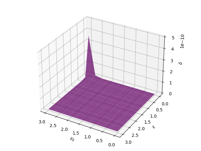
Figure 1: $\delta$ for varying $\epsilon$ and $\epsilon_{0}$ for the synthetic data. The figure shows the trend that we would expect: $\delta$ increases as $\epsilon_{0}$ increases and decreases as $\epsilon$ increases.

V-C2 Comparing the utility of the shuffle and the central models

In this section, we compare the utilities of the central model and the shuffle models, providing the same level of privacy protection. For neutral comparison, we perform the experiments into two cases: individual specific utility and community level utility, as described earlier in this section. We use the total variation distance to estimate the difference between original distribution and estimated distributions.

TABLE V: Comparing the individual specific utility $\overline{\mathcal{W}}$ of the central and the shuffle models for synthetic data ($\epsilon=4$)

$x_{0}$	$n=1,000$		$n=100,000$
	Gaussian	shuffle+INV	Gaussian	shuffle+INV
1	3E-3	1E-3	6E-6	3E-3
3	6E-4	2E-4	1E-5	5E-4
5	12E-4	11E-4	1E-5	5E-4
7	1E-4	4E-3	8E-6	3E-5
9	9E-4	3E-3	7E-6	8E-4
11	6E-4	1E-3	6E-6	7E-4
13	15E-4	15E-4	2E-5	4E-4

Table V shows the results from the experimental analysis of comparing the individual specific utilities $\overline{\mathcal{W}}$ of the shuffle model + INV ($\mathcal{M}$) and the central model with Gaussian noise ($\mathfrak{N}$), as the primary input $x_{0}$ changes its value. We performed the experiments for the case of $n=1,000$ and $n=100,000$, setting $\epsilon_{0}=4$, $\epsilon=4$, and $k=15$, calculating $\delta$ for each $x_{0}$. When $n=1,000$, shuffle+INV is comparable with the optimal Gaussian mechanism, depending on the value of $x_{0}$. However, when $n$ is $100,000$, the Gaussian mechanism shows better results regardless of $x_{0}$. This is explained through our choice of $\delta$ (given by Theorem IV.1), which depends on $n_{x_{0}}$, which, in turn, varies with $x_{0}$ and that Gaussian mechanism inserts fixed noise regardless of $n$. However, even for a large value of $n$, the utility of shuffle-INV, although slightly worse than that of the optimal Gaussian mechanism, is quite good as $\overline{\mathcal{W}}(\mathcal{M},x_{0})$ remains very low across different $x_{0}$.

For the community level utility, we apply the worst case (highest value) of $\delta$ computed over all the primary inputs for all the users in $\mathfrak{U}$, given as $\hat{\delta}$ in (10), to sanitize all input messages of the dataset – thus establishing the worst tight ADP guarantee possible on the shuffle model. This is used to determine the community level utility of the corresponding shuffle model with the estimated differential privacy guarantee. Similar to the case of individual specific utility, experiments were performed for the case of $n=1,000$ and $n=100,000$, and the other parameters used for the experiment being the same. When $n=1,000$, total variation distance between the original distribution and that of the noisy data obtained with Gaussian mechanism is 0.014, and correspondingly between the original distribution and that obtained with shuffle+INV is 0.026. When $n=100,000$, total variation distance between the original distribution and that of the noisy data obtained with Gaussian mechanism is 0.0001, and that for shuffle+INV is 0.0048. This is similar to what we showed for individual specific utility. When $n$ is small, the utility of shuffle model is almost as much as that of the central model. As $n$ increases, the utility of the Gaussian mechanism, $\mathfrak{N}$, improves slightly over that of the shuffle model under the same level of differential privacy, however they still are fairly close.

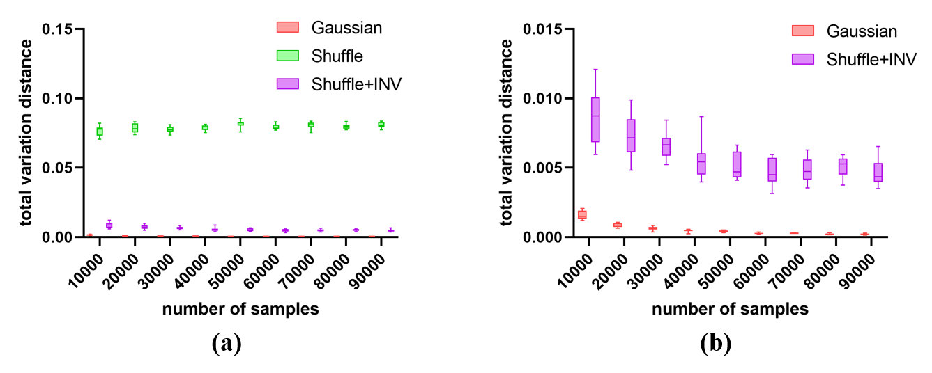
Figure 2: (a): TV distance of the original dist. with Gaussian and that with shuffle and shuffle+INV, illustrating the comparison of community level utilities between Gaussian and shuffle models for varying $n$. (b): Illustrates results of just the Gaussian and shuffle+INV for clarity.

Figure 2 shows the result of comparing the original distribution of the data with the Gaussian mechanism, shuffle model with $k$-RR and shuffle+INV while varying $n$. We set the other parameters as follows: $k=15$,  $\epsilon=4$, and $\hat{\delta}$ in (10) for the Gaussian mechanism. We observe that the utility for shuffle+INV shows better utility than shuffle model with $k$-RR, and the utility for the shuffle+INV is slightly worse than the central model in our notion of utility, as we would expect from the literature. We can draw conclusion from the experimental results that keeping the other parameters fixed, shuffle model shows worse utility than central model, but it is comparable especially when the number of samples is small and the privacy level is low.

V-D Results on real data

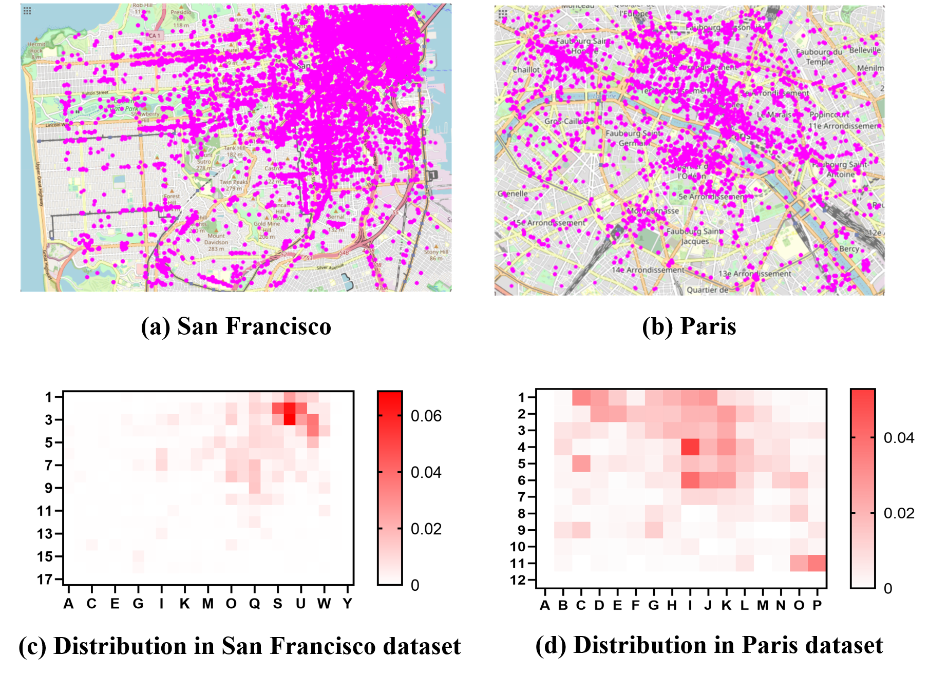
Figure 3: (a): Location data from Gowalla check-ins from a northern part of San Francisco. (b): Location data from Gowalla check-ins from a part of Paris. (c) and (d) give the heatmap of the locations in the areas of San Francisco and Paris as an alternative visualization.

Now we focus on the experimental results obtained using real location data from Gowalla dataset[31, 32]. We consider the data from: (i) a northern part of San Francisco bounded by latitudes (37.7228, 37.7946) and longitudes (-122.5153, -122.3789) covering an area of 12Km$\times$8Km, discretized with $24\times 17$ grid; (ii) Paris bounded by latitudes (48.8286, 48.8798), and longitudes (2.2855, 2.3909) covering 8Km$\times$6Km, discretized with $16\times 12$ grid. We use 123,108 check-in locations from Gowalla dataset in San Francisco and 10,260 check-ins in Paris. Figures 3 (a) and 3 (b) show the original check-in data derived from the Gowalla dataset, and the magenta dots on the region represents the particular data points (locations).

Figures 4 and 5 illustrate the estimations of the original distributions of location data from San Francisco and Paris, respectively. We sanitize the original distribution using shuffle model giving a tight differential privacy guarantee with parameters $\epsilon$ and $\hat{\delta}$, as in (10). We use the same $\epsilon$ and $\hat{\delta}$ to privatize the original data using the Gaussian mechanism [30, 7], same as in the previous experiment, thus getting a $(\epsilon,\,\hat{\delta})$-DP guarantee for both the cases.

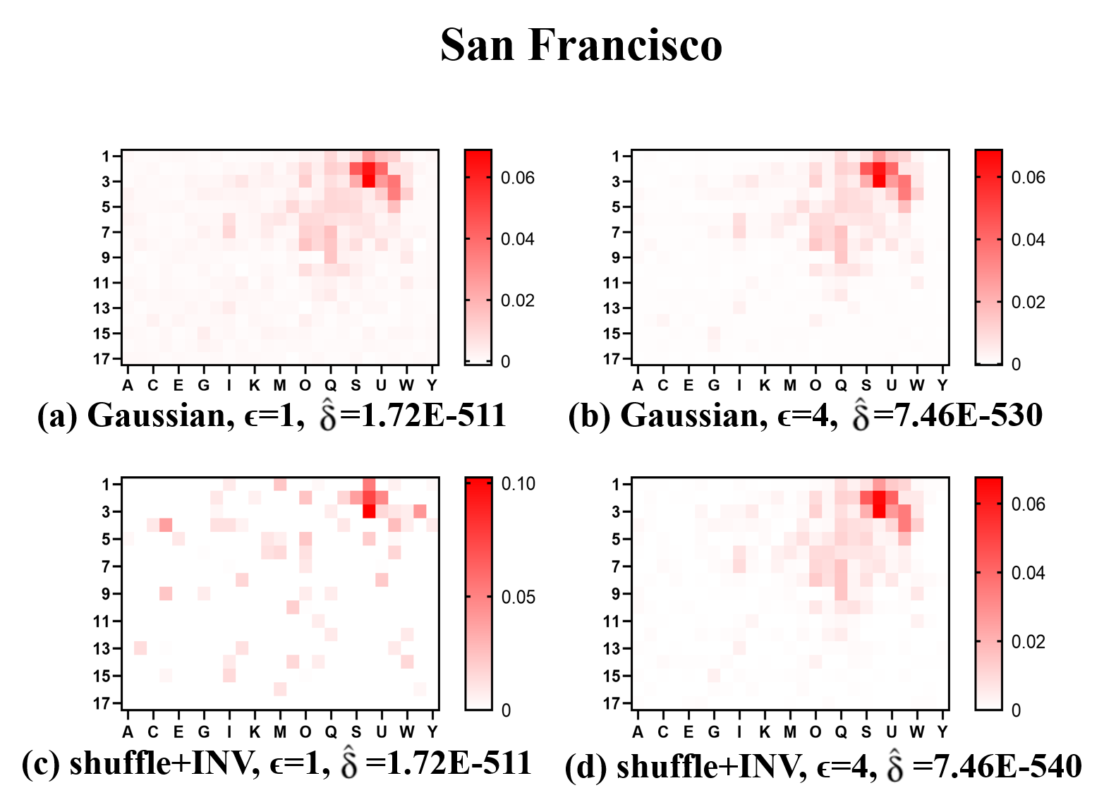
Figure 4: Estimation of the original distribution from the noisy data obfuscated with the Gaussian mechanism and the shuffle model in San Francisco dataset

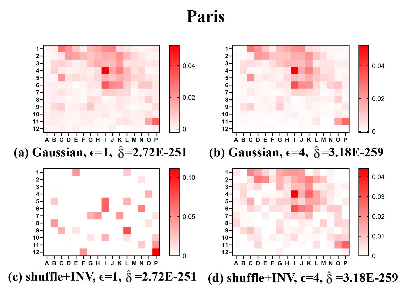
Figure 5: Estimation of the original distribution from the noisy data obfuscated with the Gaussian mechanism and the shuffle model in Paris dataset

To compare the utility of the two mechanisms under the same privacy level, we estimate the original distributions – using shuffle+INV for the shuffle model and the Gaussian mechanism itself for the central model, as described in (8) and (9) – and evaluate how “far” the corresponding estimations lie from the original distributions. We observe that Gaussian mechanism approximates the original distributions slightly better than the shuffle+INV in all cases, but it is comparable.

As we observe in the previous experiment results, the number of samples, $\epsilon$ affect the utility. In Figures 6 and 7, we show how the number of samples and the differential privacy parameters affect the utilities in more detail. In summary, we observe a consistency with the existing work in the trend of the Gaussian mechanism having a better utility than the shuffle model across all settings. However, when the number of samples is small and the privacy level is low, the utilities of the shuffle model and the central model are comparable.

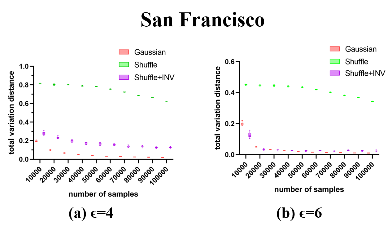
Figure 6: (a), (b): TV distance of the original dist. with Gaussian, that with shuffle and shuffle+INV, illustrating the comparison of community level utilities between Gaussian, shuffle and shuffle+INV for varying $n$ and varying $\epsilon$ in San Francisco dataset.

Figures 6 (a) and 6 (b) illustrate the evaluation the TV distance between the original and the estimated distributions for San Francisco dataset. $n$ ranges from $10,000$ to $100,000$, which is used to sample locations from the aforementioned San Francisco region. We set $\epsilon=4$ and $\epsilon=6$ to capture the change of distance between the original and the estimated distributions by varying $n$. We use $\hat{\delta}$, as in (10), to calculate community level utility and we run the mechanism 10 times to obtain the boxplots. The results exhibit that shuffle model$,\mathcal{M}$, gives worse utility than the central model $\mathfrak{N}_{\epsilon,\hat{\delta}}$, and shuffle+INV shows better utility than shuffle. This trend is harmonious across the different settings for $\epsilon$. It is reassuring to observe that the shuffle+INV is slightly closer or comparable with the Gaussian mechanism especially when the value of $n$ is small ($n=10,000$) and privacy level is low ($\epsilon=6$).

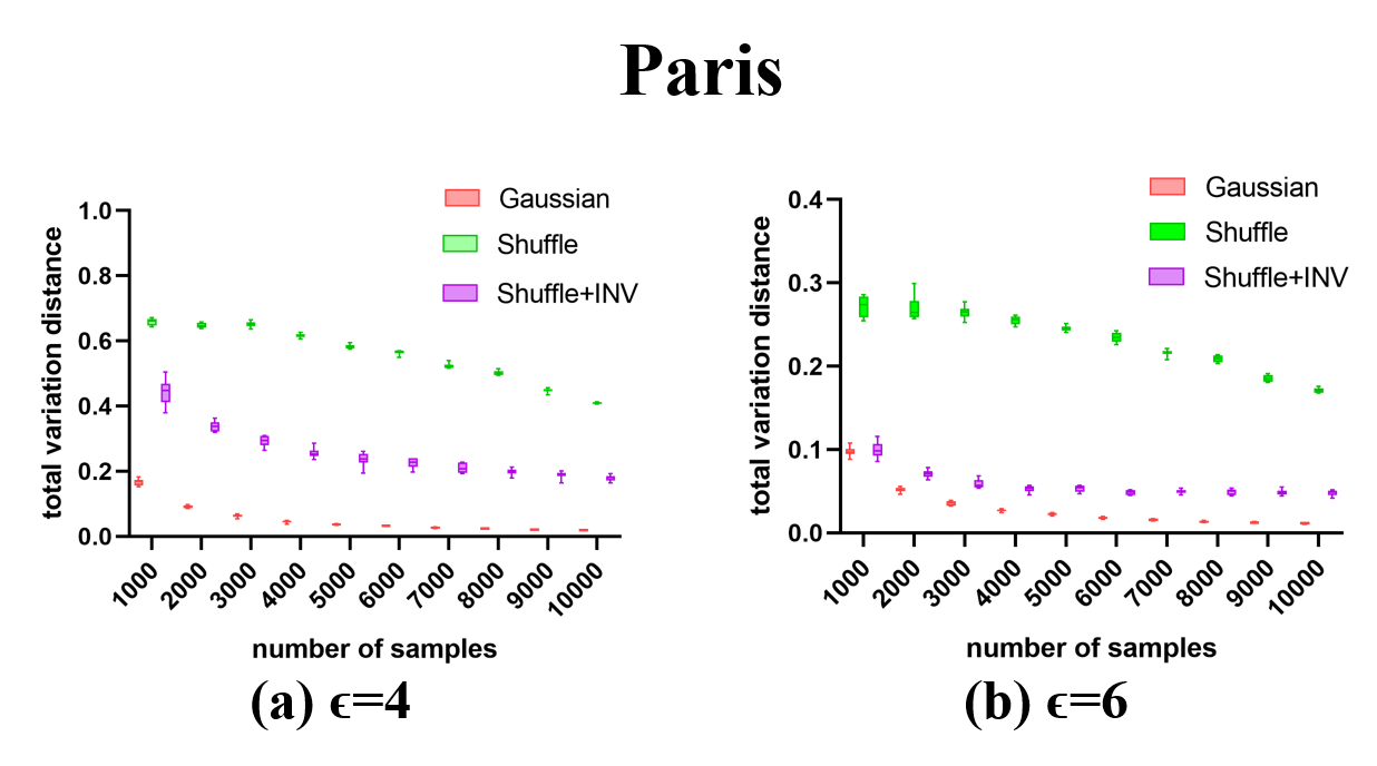
Figure 7: (a) and (b) show the TV distance of the original dist. with Gaussian, that with shuffle and shuffle+INV, illustrating the comparison of community level utilities between Gaussian, shuffle and shuffle+INV for varying $n$ and varyng $\epsilon$ in Paris dataset.

Figure 7 shows the TV distance between the estimated and the original distributions and the utility difference for locations in Paris from Gowalla dataset with $n$ ranging from 1,000 to 10,000 and the other parameters being the same as the experiments for the San Francisco dataset.

The overall trend of TV distance for the dataset of Paris is the same as that of San Francisco. Again, we observe that the utility of the shuffle+INV is better than that of just shuffle with $k$-RR, and the utilities of the shuffle+INV and the optimal Gaussian mechanism are almost indistinguishable when the number of samples and the privacy level are low. As we see from the heatmaps in Figure 4 and Figure 5, when the value of $\epsilon$ is 4, both Gaussian mechanism and shuffle+INV generate results very close to the original distribution. Individual specific utilities for Paris and San Francisco dataset are described in Table VI.

TABLE VI: Individual specific utility comparison of central and shuffle models for Gowalla data ($\epsilon=4$, $\epsilon_{0}=4$)

$x_{0}$	San Francisco		$x_{0}$	Paris
	Gaussian	shuffle+INV		Gaussian	shuffle+INV
40	4E-6	1E-3	20	2E-6	3E-4
80	3E-5	5E-4	40	3E-5	2E-3
120	9E-6	1E-3	60	4E-5	2E-3
160	4E-5	2E-4	80	5E-5	4E-4
200	2E-5	2E-4	100	7E-5	1E-4
240	2E-5	7E-4	120	3E-5	2E-4
280	4E-6	5E-4	140	1E-4	1E-4

VI Conclusion

In this paper, we have compared the privacy-utility trade-off of two different models of differential privacy for histogram queries: the classic central model with the optimal Gaussian mechanism and the shuffle model with $k$-RR mechanism as the local randomizer, enhanced with a post-processing to de-noise the resulting histogram. In order to do this comparison, we needed to derive strictest bounds for the level of privacy provided by the shuffle model, so that we could tune the parameters of the Gaussian mechanism to provide the same privacy.

First, we have used a result on the condition for tightness of ADP given by Sommer et al. in [6] and translated it in the context of shuffle models, giving rise to a closed form expression of the least $\delta$ for any $\epsilon$ and, thus, we obtained a necessary and sufficient condition to have the tightest DP guarantee for the shuffle models. This result shows that the differential privacy ensured by the shuffle models under a certain level of local noise is much higher than what has been known by the community so far.

Then, we have adapted the matrix inversion method to the noisy histogram output of the shuffle model, in order to reduce the noise and hence increase the utility.

Finally we have performed experiments on synthetic and real location data from San Francisco and Paris, and we have compared the statistical utilities of the shuffle and the central models. We observed that, although the central model still performs better than the shuffle model, but only ever so slightly – the gap between their statistical utilities is very small, and tend to vanish as the number of samples increases. Combining this result with the fact that the shuffle model effaces the need of having a trusted central curator to sanitize the original datasets, we conclude that the shuffle model is much more convenient than the central one for the privacy-preserving release of histograms.

We plan on studying more generalized forms of shuffle models using different local randomizers and comparing their utilities with the central models. We would also like to extend the notion of utility, beyond what we used in this paper, and analyse the behaviour of shuffle models with other renditions of differential privacy.

Appendix A Proofs

See IV.1

Proof.

Setting $p=\mathbb{P}(x_{0}|x_{0})$ and $\overline{p}=\mathbb{P}(x_{0}|y\neq x_{0})$ in $\mathcal{R}_{\text{kRR}}$, for any $s\in\{0,\ldots,n\}$:

$$\mathbb{P}(\mathcal{M}_{x_{0}}(x_{0})=s)=p\sum\limits_{r=0}^{s-1}\left[\binom{n_{x_{0}}}{r}p^{r}(1-p)^{n_{x_{0}}-r}\right.$$

$$\times\left.\binom{n-1-n_{x_{0}}}{s-1-r}\overline{p}^{s-1-r}(1-\overline{p})^{n-n_{x_{0}}-s+r}\right]$$

$$+(1-p)\sum\limits_{r=0}^{s}\left[\binom{n_{x_{0}}}{r}p^{r}(1-p)^{n_{x_{0}}-r}\right.$$

$$\times\left.\binom{n-1-n_{x_{0}}}{s-r}\overline{p}^{s-r}(1-\overline{p})^{n-n_{x_{0}}-1-s+r}\right]$$

$$=\frac{e^{\epsilon_{0}}}{e^{\epsilon_{0}}+k-1}\sum\limits_{r=0}^{s-1}\left[\binom{n_{x_{0}}}{r}\frac{e^{r\epsilon_{0}}(k-1)^{n_{x_{0}}-r}}{(e^{\epsilon_{0}}+k-1)^{n_{x_{0}}}}\right.$$

$$\times\left.\binom{n-1-n_{x_{0}}}{s-1-r}\frac{(e^{\epsilon_{0}}+k-2)^{n-n_{x_{0}}-s+r}}{(e^{\epsilon_{0}}+k-1)^{n-1-n_{x_{0}}}}\right]$$

$$+\frac{k-1}{e^{\epsilon_{0}}+k-1}\sum\limits_{r=0}^{s}\left[\binom{n_{x_{0}}}{r}\frac{e^{r\epsilon_{0}}(k-1)^{n_{x_{0}}-r}}{(e^{\epsilon_{0}}+k-1)^{n_{x_{0}}}}\right.$$

$$\times\left.\binom{n-1-n_{x_{0}}}{s-r}\frac{(e^{\epsilon_{0}}+k-2)^{n-n_{x_{0}}-1-s+r}}{(e^{\epsilon_{0}}+k-1)^{n-1-n_{x_{0}}}}\right]$$

$$=\frac{e^{\epsilon_{0}}(k-1)^{n_{x_{0}}}(e^{\epsilon_{0}}+k-2)^{n-n_{x_{0}}-s}}{(e^{\epsilon_{0}}+k-1)^{n}}$$

$$\times\sum\limits_{r=0}^{s-1}\binom{n_{x_{0}}}{r}\binom{n-1-n_{x_{0}}}{s-1-r}\kappa_{1}^{r}$$

$$+\frac{(k-1)^{n_{x_{0}}+1}(e^{\epsilon_{0}}+k-2)^{n-n_{x_{0}}-1-s}}{(e^{\epsilon_{0}}+k-1)^{n}}$$

$$\times\sum\limits_{r=0}^{s}\binom{n_{x_{0}}}{r}\binom{n-1-n_{x_{0}}}{s-r}\kappa_{1}^{r}\text{ [$\kappa_{1}$ is as in \eqref{kappa6}]}$$

$$=\kappa_{3}\left[e^{\epsilon_{0}}\sum\limits_{r=0}^{s-1}\binom{n_{x_{0}}}{r}\binom{n-1-n_{x_{0}}}{s-1-r}\kappa_{1}^{r}\right.$$

$$+\left.\kappa_{2}\sum\limits_{r=0}^{s}\binom{n_{x_{0}}}{r}\binom{n-1-n_{x_{0}}}{s-r}\kappa_{1}^{r}\right]$$ (11)

Using elementary combinatorial identities $\eqref{freqquery2impeq}$ reduces to:

$$\kappa_{3}\left[\kappa_{2}\sum\limits_{r=0}^{s}\binom{n_{x_{0}}}{r}\kappa_{1}^{r}\left(\binom{n-1-n_{x_{0}}}{s-1-r}+\binom{n-1-n_{x_{0}}}{s-r}\right)\right.$$

$$\left.+(e^{\epsilon_{0}}-\kappa_{2})\left(e^{\epsilon_{0}}\sum\limits_{r=0}^{s-1}\binom{n_{x_{0}}}{r}\binom{n-1-n_{x_{0}}}{s-1-r}\kappa_{1}^{r}\right)\right]$$

$$=\kappa_{3}\left[\kappa_{2}\sum\limits_{r=0}^{s}\binom{n_{x_{0}}}{r}\binom{n-n_{x_{0}}}{s-r}\kappa_{1}^{r}\right.$$

$$\left.+(e^{\epsilon_{0}}-\kappa_{2})\left(\sum\limits_{r=0}^{s}\binom{n_{x_{0}}}{r}\binom{n-1-n_{x_{0}}}{s-1-r}\kappa_{1}^{r}\right)\right]$$

$$=\kappa_{3}\left[\kappa_{2}\sum\limits_{r=0}^{s}\binom{n_{x_{0}}}{r}\binom{n-n_{x_{0}}}{s-r}\kappa_{1}^{r}\right.$$

$$\left.+\frac{(e^{\epsilon_{0}}-\kappa_{2})(s-r)}{n-n_{x_{0}}}\sum\limits_{r=0}^{s}\binom{n_{x_{0}}}{r}\binom{n-n_{x_{0}}}{s-r}\kappa_{1}^{r}\right]$$

$$=\frac{\kappa_{3}}{n-n_{x_{0}}}\sum\limits_{r=0}^{s}\mu(s,r)\tau_{r}\text{ [$\mu$, $\tau$ as in Definition \ref{finaldelta}]}$$ (12)

By very similar arguments and algebra,

$$\mathbb{P}(\mathcal{M}_{x_{0}}(x_{1})=s)\text{ for some $s\in\{0,\ldots,n\}$}$$

$$\frac{1}{e^{\epsilon_{0}}+k-1}\sum\limits_{r=0}^{s-1}\left[\binom{n_{x_{0}}}{r}\frac{e^{r\epsilon_{0}}(k-1)^{n_{x_{0}}-r}}{(e^{\epsilon_{0}}+k-1)^{n_{x_{0}}}}\right.$$

$$\times\left.\binom{n-1-n_{x_{0}}}{s-r}\frac{(e^{\epsilon_{0}}+k-2)^{n-n_{x_{0}}-s+r}}{(e^{\epsilon_{0}}+k-1)^{n-1-n_{x_{0}}}}\right]$$

$$+\frac{e^{\epsilon_{0}}+k-2}{e^{\epsilon_{0}}+k-1}\sum\limits_{r=0}^{s}\left[\binom{n_{x_{0}}}{r}\frac{e^{r\epsilon_{0}}(k-1)^{n_{x_{0}}-r}}{(e^{\epsilon_{0}}+k-1)^{n_{x_{0}}}}\right.$$

$$\times\left.\binom{n-1-n_{x_{0}}}{s-1-r}\frac{(e^{\epsilon_{0}}+k-2)^{n-n_{x_{0}}-1-s+r}}{(e^{\epsilon_{0}}+k-1)^{n-1-n_{x_{0}}}}\right]$$

$$=\kappa_{3}\left(\sum\limits_{r=0}^{s}\binom{n_{x_{0}}}{r}\binom{n-1-n_{x_{0}}}{s-1-r}\kappa_{1}^{r}\right.$$

$$\left.+\sum\limits_{r=0}^{s}\binom{n_{x_{0}}}{r}\binom{n-1-n_{x_{0}}}{s-r}\kappa_{1}^{r}\right)$$

[$$\kappa_{3}$$ as in (5)]

$$=\kappa_{3}\sum\limits_{r=0}^{s}\binom{n_{x_{0}}}{r}\binom{n-n_{x_{0}}}{s-r}\kappa_{1}^{r}$$ (13)

Using Result 1, for every $k>2$ and $s\in\{0,1,\ldots,n\}$, we can say that in $\mathcal{M}$, we have a tight $(\epsilon,\,\delta)$-ADP guarantee with respect to $x_{0},\,x_{1}\in\mathcal{X}$ for any $\epsilon>0$ and $\delta$ iff $\delta$ is defined as:

$$\delta(\epsilon)=\sum\limits_{v:v>\epsilon}(1-e^{\epsilon-v})\sum\limits_{\begin{subarray}{c}s=0\\ v=\ln{\frac{\mathbb{P}(\mathcal{M}_{x_{0}}(x_{0})=s)}{\mathbb{P}(\mathcal{M}_{x_{0}}(x_{1})=s)}}\end{subarray}}^{n}\mathbb{P}(\mathcal{M}_{x_{0}}(x_{0})=s)$$ (14)

We use the expressions for $\mathbb{P}(\mathcal{M}_{x_{0}}(x_{0})=s)$ and $\mathbb{P}(\mathcal{M}_{x_{0}}(x_{1})=s)$ from (11) and (A) respectively to get:

$$v_{s}=\ln{\frac{\mathbb{P}(\mathcal{M}_{x_{0}}(x_{0})=s)}{\mathbb{P}(\mathcal{M}_{x_{0}}(x_{1})=s)}}$$

$$=\ln{\frac{e^{\epsilon_{0}}\sum\limits_{r=0}^{s-1}\binom{n_{x_{0}}}{r}\binom{n-1-n_{x_{0}}}{s-1-r}\kappa_{1}^{r}+\kappa_{2}\sum\limits_{r=0}^{s}\binom{n_{x_{0}}}{r}\binom{n-1-n_{x_{0}}}{s-r}\kappa_{1}^{r}}{\sum\limits_{r=0}^{s-1}\binom{n_{x_{0}}}{r}\binom{n-1-n_{x_{0}}}{s-1-r}\kappa_{1}^{r}+\sum\limits_{r=0}^{s}\binom{n_{x_{0}}}{r}\binom{n-1-n_{x_{0}}}{s-r}\kappa_{1}^{r}}}$$

$$=\ln{\left(\kappa_{2}+\frac{(e^{\epsilon_{0}}-\kappa_{2})\left(\sum\limits_{r=0}^{s-1}\binom{n_{x_{0}}}{r}\binom{n-1-n_{x_{0}}}{s-1-r}\kappa_{1}^{r}\right)}{\sum\limits_{r=0}^{s}\binom{n_{x_{0}}}{r}\binom{n-n_{x_{0}}}{s-r}\kappa_{1}^{r}}\right)}$$

$$=\ln{\left(\kappa_{2}+\frac{\frac{(e^{\epsilon_{0}}-\kappa_{2})}{n-n_{x_{0}}}\left(\sum\limits_{r=0}^{s}(s-r)\binom{n_{x_{0}}}{r}\binom{n-1-n_{x_{0}}}{s-1-r}\kappa_{1}^{r}\right)}{\sum\limits_{r=0}^{s}\binom{n_{x_{0}}}{r}\binom{n-n_{x_{0}}}{s-r}\kappa_{1}^{r}}\right)}$$ (15)

Combining (15) and (14), we obtain:

$$\delta(\epsilon)=\sum\limits_{u:u>\epsilon}(1-e^{\epsilon-v})\sum\limits_{\begin{subarray}{c}s=0\\ v=\ln{\frac{\mathbb{P}(\mathcal{M}_{x_{0}}(x_{0})=s)}{\mathbb{P}(\mathcal{M}_{x_{0}}(x_{1})=s)}}\end{subarray}}^{n}\mathbb{P}(\mathcal{M}_{x_{0}}(x_{0})=s)$$

$$=\sum\limits_{s=0}^{n}\mathbbm{1}_{\{v_{s}>\epsilon\}}(1-e^{\epsilon-v_{s}})\mathbb{P}(\mathcal{M}_{x_{0}}(x_{0})=s)$$

$$=\sum\limits_{s=0}^{n}\mathbbm{1}_{\{v_{s}>\epsilon\}}(1-e^{\epsilon-v_{s}})\frac{\kappa_{3}}{n-n_{x_{0}}}\sum\limits_{r=0}^{s}\mu(s,r)\tau_{r}=\hat{\delta}(\epsilon)$$

[Substituting $$\mathbb{P}(\mathcal{M}_{x_{0}}(x_{0})=s)$$ from (12)].

∎

References

- [1] C. Dwork, “Differential privacy,” in International Colloquium on Automata, Languages, and Programming, pp. 1–12, Springer, 2006.
- [2] C. Dwork, K. Kenthapadi, F. McSherry, I. Mironov, and M. Naor, “Our data, ourselves: Privacy via distributed noise generation,” in Advances in Cryptology - EUROCRYPT 2006 (S. Vaudenay, ed.), (Berlin, Heidelberg), pp. 486–503, Springer Berlin Heidelberg, 2006.
- [3] C. Dwork, F. McSherry, K. Nissim, and A. Smith, “Calibrating noise to sensitivity in private data analysis,” in Theory of Cryptography (S. Halevi and T. Rabin, eds.), (Berlin, Heidelberg), pp. 265–284, Springer Berlin Heidelberg, 2006.
- [4] J. C. Duchi, M. I. Jordan, and M. J. Wainwright, “Local privacy and statistical minimax rates,” in 2013 IEEE 54th Annual Symposium on Foundations of Computer Science, pp. 429–438, IEEE, 2013.
- [5] A. Bittau, Ú. Erlingsson, P. Maniatis, I. Mironov, A. Raghunathan, D. Lie, M. Rudominer, U. Kode, J. Tinnes, and B. Seefeld, “Prochlo: Strong privacy for analytics in the crowd,” in Proceedings of the 26th Symposium on Operating Systems Principles, pp. 441–459, 2017.
- [6] D. M. Sommer, S. Meiser, and E. Mohammadi, “Privacy loss classes: The central limit theorem in differential privacy,” Proceedings on privacy enhancing technologies, vol. 2019, no. 2, pp. 245–269, 2019.
- [7] B. Balle and Y.-X. Wang, “Improving the gaussian mechanism for differential privacy: Analytical calibration and optimal denoising,” in International Conference on Machine Learning, pp. 394–403, PMLR, 2018.
- [8] P. Kairouz, K. Bonawitz, and D. Ramage, “Discrete distribution estimation under local privacy,” in International Conference on Machine Learning, pp. 2436–2444, PMLR, 2016.
- [9] A. Cheu, “Differential privacy in the shuffle model: A survey of separations,” arXiv preprint arXiv:2107.11839, 2021.
- [10] B. Balle, J. Bell, A. Gascón, and K. Nissim, “The privacy blanket of the shuffle model,” in Annual International Cryptology Conference, pp. 638–667, Springer, 2019.
- [11] Ú. Erlingsson, V. Feldman, I. Mironov, A. Raghunathan, K. Talwar, and A. Thakurta, “Amplification by shuffling: From local to central differential privacy via anonymity,” in Proceedings of the Thirtieth Annual ACM-SIAM Symposium on Discrete Algorithms, pp. 2468–2479, SIAM, 2019.
- [12] V. Feldman, A. McMillan, and K. Talwar, “Hiding among the clones: A simple and nearly optimal analysis of privacy amplification by shuffling,” arXiv preprint arXiv:2012.12803, 2020.
- [13] Ú. Erlingsson, V. Feldman, I. Mironov, A. Raghunathan, S. Song, K. Talwar, and A. Thakurta, “Encode, shuffle, analyze privacy revisited: Formalizations and empirical evaluation,” arXiv preprint arXiv:2001.03618, 2020.
- [14] B. Balle, J. Bell, A. Gascon, and K. Nissim, “Differentially private summation with multi-message shuffling,” arXiv preprint arXiv:1906.09116, 2019.
- [15] B. Balle, J. Bell, A. Gascón, and K. Nissim, “Private summation in the multi-message shuffle model,” in Proceedings of the 2020 ACM SIGSAC Conference on Computer and Communications Security, pp. 657–676, 2020.
- [16] A. Cheu, A. Smith, J. Ullman, D. Zeber, and M. Zhilyaev, “Distributed differential privacy via shuffling,” in Annual International Conference on the Theory and Applications of Cryptographic Techniques, pp. 375–403, Springer, 2019.
- [17] Y. Ishai, E. Kushilevitz, R. Ostrovsky, and A. Sahai, “Cryptography from anonymity,” in 2006 47th Annual IEEE Symposium on Foundations of Computer Science (FOCS’06), pp. 239–248, IEEE, 2006.
- [18] B. Ghazi, R. Pagh, and A. Velingker, “Scalable and differentially private distributed aggregation in the shuffled model,” arXiv preprint arXiv:1906.08320, 2019.
- [19] B. Balle, J. Bell, A. Gascón, and K. Nissim, “Improved summation from shuffling,” arXiv preprint arXiv:1909.11225, 2019.
- [20] V. Balcer and A. Cheu, “Separating local & shuffled differential privacy via histograms,” arXiv preprint arXiv:1911.06879, 2019.
- [21] A. Cheu and M. Zhilyaev, “Differentially private histograms in the shuffle model from fake users,” arXiv preprint arXiv:2104.02739, 2021.
- [22] V. Balcer, A. Cheu, M. Joseph, and J. Mao, “Connecting robust shuffle privacy and pan-privacy,” in Proceedings of the 2021 ACM-SIAM Symposium on Discrete Algorithms (SODA), pp. 2384–2403, SIAM, 2021.
- [23] A. Cheu and J. Ullman, “The limits of pan privacy and shuffle privacy for learning and estimation,” in Proceedings of the 53rd Annual ACM SIGACT Symposium on Theory of Computing, pp. 1081–1094, 2021.
- [24] A. Koskela, M. A. Heikkilä, and A. Honkela, “Tight accounting in the shuffle model of differential privacy,” arXiv preprint arXiv:2106.00477, 2021.
- [25] A. Koskela, J. Jälkö, L. Prediger, and A. Honkela, “Tight differential privacy for discrete-valued mechanisms and for the subsampled gaussian mechanism using fft,” in International Conference on Artificial Intelligence and Statistics, pp. 3358–3366, PMLR, 2021.
- [26] C. Dwork, A. Roth, et al., “The algorithmic foundations of differential privacy.,” Foundations and Trends in Theoretical Computer Science, vol. 9, no. 3-4, pp. 211–407, 2014.
- [27] R. Agrawal, R. Srikant, and D. Thomas, “Privacy preserving olap,” in Proceedings of the 2005 ACM SIGMOD international conference on Management of data, pp. 251–262, 2005.
- [28] D. Agrawal and C. C. Aggarwal, “On the design and quantification of privacy preserving data mining algorithms,” in Proceedings of the twentieth ACM SIGMOD-SIGACT-SIGART symposium on Principles of database systems, pp. 247–255, 2001.
- [29] W. Wang and M. A. Carreira-Perpinán, “Projection onto the probability simplex: An efficient algorithm with a simple proof, and an application,” arXiv preprint arXiv:1309.1541, 2013.
- [30] N. Holohan, S. Braghin, P. Mac Aonghusa, and K. Levacher, “Diffprivlib: the IBM differential privacy library,” ArXiv e-prints, vol. 1907.02444 [cs.CR], July 2019.
- [31] E. Cho, S. A. Myers, and J. Leskovec, “Friendship and mobility: user movement in location-based social networks,” in Proceedings of the 17th ACM SIGKDD international conference on Knowledge discovery and data mining, pp. 1082–1090, 2011.
- [32] “The gowalla dataset. [online].” https://snap.stanford.edu/data/loc-gowalla.html, 2011. (Accessed on 10/08/2021).