Controlling the shape of small clusters with and without macroscopic fields

Abstract

Despite major advances in the understanding of the formation and dynamics of nano-clusters in the past decades, theoretical bases for the control of their shape are still lacking. We investigate strategies for driving fluctuating few-particle clusters to an arbitrary target shape in minimum time with or without an external field. This question is recast into a first passage problem, solved numerically, and discussed within a high temperature expansion. Without field, large-enough low-energy target shapes exhibit an optimal temperature at which they are reached in minimum time. We then compute the optimal way to set an external field to minimize the time to reach the target, leading to a gain of time that grows when increasing cluster size or decreasing temperature. This gain can shift the optimal temperature or even create one. Our results could apply to clusters of atoms at equilibrium, and colloidal or nanoparticle clusters under thermo- or electrophoresis.

Less than a decade after its discovery Binnig and Rohrer (1983), scanning tunneling microscope (STM) was used to position atoms on a surface with Ånsgtrom precision Eigler and Schweizer (1990), reaching atomic-scale control on the organization of matter. Following this seminal work, many examples of organization of atoms Cooper et al. (2018); Barredo et al. (2016), molecules or nanoparticles Martínez-Galera et al. (2014); Erickson et al. (2011); Junno et al. (1995); Baur et al. (1998); Rubio-Sierra et al. (2005) and colloids Korda et al. (2002); Grier (2003) were obtained with tools like STM, atomic force microscope, or optical tweezers. However, important challenges are still open in the control of few-particle clusters.

The first one is to control matter at the nanoscale with an external macroscopic field that does not act on one single particle or atom at a time, but on the whole cluster. External fields such as light acting on metal nanoparticle clusters McCormack et al. (2018) or electromigration acting on atomic monolayer clusters Kuhn et al. (2005); Mahadevan and Bradley (1999); Pierre-Louis and Einstein (2000); Curiotto et al. (2019) are known to lead to complex equilibrium or non-equilibrium cluster shapes. However, these shapes are only a very small fraction of all possible shapes, that are dictated by the physics of the interaction of the driving force with the system.

Another challenge lies in the ability to obtain refined control of nanostructure shapes in the presence of thermal fluctuations that activate the random diffusion of particles and atoms, leading to shape fluctuations Khare et al. (1995); Pierre-Louis and Einstein (2000); Lai et al. (2017). Some progress in this direction has been achieved with the control of the formation and order of colloidal clusters Juárez and Bevan (2012); Juárez et al. (2012); Xue et al. (2014) in finite-temperature experiments. However, the control of the cluster shape is still an open issue.

In order to address these challenges, we investigate strategies to reach arbitrary cluster shapes in minimum time in the presence of fluctuations. We focus on the control of few-particles two-dimensional clusters and find how a given target shape can be reached in minimum time with and without macroscopic external field. This problem which is formulated as the minimization of a first passage time on the graph of cluster configurations, is solved numerically and studied analytically with the help of a high temperature expansion.

In the absence of field, we find that large compact target shapes exhibit an optimal temperature at which they can be reached in minimum time. In the presence of an external field we use dynamic programming Sutton and Barto (2018); Bellman (2003) to find the optimal way to set the external field as a function of the cluster shape to reach the target in minimum time. The gain in time due to the forces increases with decreasing temperature and with increasing clusters size. This gain can shift the optimal temperature, or create one when it does not exist in the absence of forces.

We focus on clusters with edge diffusion dynamics. Edge diffusion was observed in metal atomic monolayer islands Giesen (2001); Tao et al. (2010), and for colloids Hubartt and Amar (2015). However, our strategy can readily be extended to any type of dynamics that preserve the number of particles such as surface-diffusion dynamics inside vacancy clusters Plass et al. (2001); Heinonen et al. (1999); Leroy et al. (2020), or dislocation-mediated cluster rearrangements in colloids VanSaders and Glotzer (2021) and metal nanoclusters Huang et al. (2018); Trushin et al. (2001). We discuss possible experiments with clusters of atoms or colloids.

Model.

We consider a small cluster on a square lattice with lattice parameter $a$ and nearest-neighbor bonds $J$ under an external macroscopic force $\bm{F}$. We assume that the current configuration of the cluster, hereafter denoted as the state $s$, can be observed at all times. The force is chosen as a function of $s$. This choice is encoded in the policy ${\bm{\phi}}$, so that $\bm{F}={\bm{\phi}}(s)$. The state $s$ can change to another state $s^{\prime}$ via the motion of a single particle to one of its nearest or next-nearest neighbor sites along the cluster edge. Moves that break the cluster are forbidden. Following usual models for biased diffusion Glasstone et al. (1941); Liu and Weeks (1998); Pierre-Louis and Einstein (2000), the hopping rate is assumed to take an Arrhenius form

$$\gamma_{\bm{\phi}}(s,s^{\prime})=\nu\exp[-(n_{ss^{\prime}}J-{\bm{\phi}}(s)\cdot\bm{u}_{ss^{\prime}})/k_{B}T],$$ (1)

where $k_{B}T$ is the thermal energy and $\nu$ is an attempt frequency, $n_{ss^{\prime}}$ is the number of in-plane nearest neighbors in state $s$ before hopping. To gain computation time, we freeze atoms with $n_{ss^{\prime}}=4$. In addition, we assume that the displacement vector to the diffusion saddle point $\bm{u}_{ss^{\prime}}$ is half the displacement vector between the initial and final positions of the moving atom Pierre-Louis and Einstein (2000). In the following, we choose units where $k_{B}=1$, $J=1$, $\nu=1$ and $a=1$.

Our goal is to study the time to reach a target cluster configuration $\bar{s}$ from an initial state $s$. This time can be seen as a first passage time $\tau_{\bm{\phi}}(s,{\bar{s}})$ in a random walk on the graph of cluster configurations Sanchez and Evans (1999); Combe and Larralde (2000), as represented in Fig. 1. Since the dynamics is Markovian, $\tau_{\bm{\phi}}(s,{\bar{s}})$ is equal to the expected residence time $t_{\bm{\phi}}(s)$ in state $s$ plus the first passage time from the new state $s^{\prime}$ after the move Van Kampen (1992). Considering all possible moves, we obtain a recursion relation

$$\tau_{\bm{\phi}}(s,{\bar{s}})=t_{\bm{\phi}}(s)+\!\sum_{s^{\prime}\in{\cal B}_{s}}\!p_{\bm{\phi}}(s,s^{\prime})\tau_{{\bm{\phi}}}(s^{\prime},{\bar{s}})\,,$$ (2)

where $p_{\bm{\phi}}(s,s^{\prime})=\gamma_{\bm{\phi}}(s,s^{\prime})\,t_{\bm{\phi}}(s)$ is the transition probability from $s$ to $s^{\prime}$, $t_{\bm{\phi}}(s)=1/\!\sum_{s^{\prime}\in{\cal B}_{s}}\!\gamma_{\bm{\phi}}(s,s^{\prime})$, and ${\cal B}_{s}$ the set of states that can be reached from $s$ via a single move. Relation Eq. (2) is supplemented with the boundary condition $\tau_{\bm{\phi}}(\bar{s},{\bar{s}})=0$.

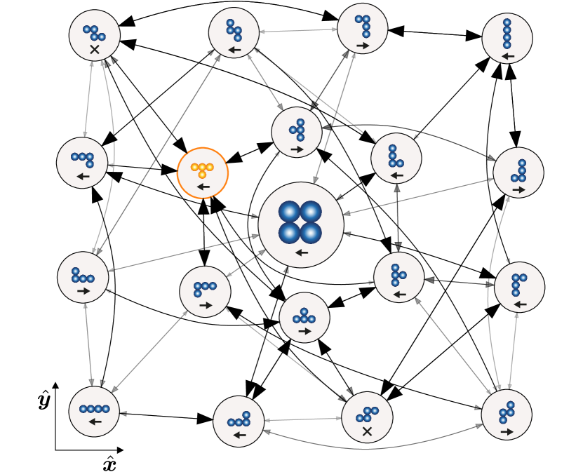
Figure 1: Graph of configurations for a tetramer cluster ($N=4$) at $T=0.24$. The node size is proportional to the expected residence time $t_{\bm{\phi}}(s)$. The thickness and shade of the edges are proportional to the transition probability $p_{\bm{\phi}}(s,s^{\prime})$. Arrows in the nodes represent an optimal policy ${\bm{\phi}}_{*}(s)$ to reach the orange target shape (crosses correspond to a zero force).

We also define the expected return time to target, i.e. spent outside the target before returning to it when starting from the target itself 

$$\tau_{\bm{\phi}}^{\mathrm{r}}({\bar{s}})=\sum_{s\in{\cal B}_{\bar{s}}}p_{\bm{\phi}}(\bar{s},s)\,\tau_{\bm{\phi}}(s,{\bar{s}})\,.$$ (3)

For the sake of concision, we mainly focus on the analysis of $\tau_{\bm{\phi}}^{\mathrm{r}}({\bar{s}})$ instead of $\tau_{\bm{\phi}}(s,{\bar{s}})$ which is different for each $s$.

Zero force.

Let us first set the force to zero in all states, ${\bm{\phi}}(s)={\bm{0}}$. This leads to standard equilibrium fluctuation dynamics that have been investigated thoroughly in the case of edge diffusion Khare et al. (1995); Giesen (2001); Lai et al. (2017). Although some quantities related to first passage processes have been discussed within the frame of persistence of fluctuations Dougherty et al. (2002); Constantin et al. (2003), there is to our knowledge no study of the first passage times to cluster configurations. We have evaluated $\tau_{\bm{\phi}}(s,{\bar{s}})$ numerically using the method of iterative evaluation Sutton and Barto (2018): for a given $\bar{s}$, we iterate the evaluation of $\tau_{{\bm{\phi}}}(s,{\bar{s}})$ by substitution of its value in the right hand side of Eq. (2). Since it requires to list all states, such a method is suitable for small clusters, which corresponds to our focus in this Letter. Indeed, the total number $S_{N}$ of configurations for a cluster with $N$ particles, often called polyominoes or lattice animals Guttmann (2009), grows exponentially with $N$: $S_{N}\sim c\lambda^{N}/N$, with $\lambda\approx 4.0626$ and $c\approx 0.3169$ Jensen and Guttmann (2000). We have performed simulations with $N\leq 12$, with $S_{12}\approx 5\times 10^{5}$ states.

The resulting expected return time to target with zero force $\tau_{0}^{\mathrm{r}}({\bar{s}})$ is shown in Fig. 2 as a function of $1/T$. For small clusters, $\tau_{0}^{\mathrm{r}}({\bar{s}})$ increases monotonously as the temperature is decreased. This is expected because thermally activated hopping diffusion events become slower at low temperatures. However, $\tau_{0}^{\mathrm{r}}({\bar{s}})$ exhibits a minimum as a function of temperature for clusters that are larger and more compact. As shown in Supp. Mat., a similar minimum is found in the time $\tau_{0}(s,{\bar{s}})$ to reach the target starting from any state $s$. This striking result implies that some targets exhibit an optimal temperature at which the target can be reached in minimum time.

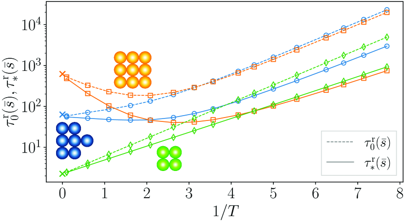
Figure 2: Expected return time to target as a function of $1/T$. Zero-force case $\tau^{\mathrm{r}}_{0}({\bar{s}})$ and under the optimal policy $\tau^{\mathrm{r}}_{*}({\bar{s}})$ with $F_{0}=0.4$. The $\times$ correspond to $\tau_{\infty}^{\mathrm{r}}(\bar{s})$ for $T\rightarrow\infty$.

The presence of a minimum is associated to a change of slope of $\tau_{0}^{\mathrm{r}}({\bar{s}})$ as a function of $1/T$ at high temperatures. We therefore study the high temperature behavior in more details. In the limit $T\rightarrow\infty$, the rates (1) are independent of the initial and final state and of the force: $\gamma_{\bm{\phi}}(s,s^{\prime})\rightarrow 1$. As a consequence, $\tau_{\bm{\phi}}^{\mathrm{r}}({\bar{s}})$ is independent of the policy ${\bm{\phi}}$ at infinite temperature $\tau_{\bm{\phi}}^{\mathrm{r}}({\bar{s}})\rightarrow{\tau}^{\mathrm{r}}_{\infty}({\bar{s}})$. A simple result is known from the literature Lovász (1993) (see also Supp. Mat.) when all rates are equal: ${\tau}^{\mathrm{r}}_{\infty}({\bar{s}})=(S_{N}-1)/d_{\bar{s}}$, where the degree $d_{\bar{s}}$ of the target is the number of states that can be reached from the target $\bar{s}$ in one move. This quantity is similar to the lower bound of the mean first passage time (averaged over all initial states $s$), which is often used to characterize first passages in random graphs Lin et al. (2012); Tejedor et al. (2009); Baronchelli and Loreto (2006); Noh and Rieger (2004).

When the temperature is decreased, the moves become sensitive to the energy. From detailed balance, a move that leads to a decrease of energy is faster than the reverse move. As a consequence, the cluster goes faster towards states with lower energy. Thus, the time to reach the target decreases if the target has a lower energy. However, this trend is only describing relative variations of the time to reach different targets. When decreasing the temperature, there is also a global slowing-down of the dynamics because of the Arrhenius dependence of the rates on temperature in Eq. (1). The decrease or increase of first passage times to the target—or equivalently of $\tau_{\bm{\phi}}^{\mathrm{r}}(\bar{s})$—depends on the competition between these two effects: relative energy effect vs global slowing down.

This competition can be analyzed from a high temperature expansion to first order in $1/T$ (details are reported in Supp. Mat.), leading to

$$\tau^{\mathrm{r}}_{0}({\bar{s}}) =\left(1+\frac{M_{0}({\bar{s}})}{T}\right)\tau^{\mathrm{r}}_{\infty}({\bar{s}})\,,$$ (4)

$$M_{0}({\bar{s}}) =\frac{1}{1-S_{N}^{-1}}\Bigl{\langle}\tilde{\delta}_{s\bar{s}}\langle n_{ss^{\prime}}\rangle_{\prime}-d_{s}g_{n}(s,{\bar{s}})\Bigr{\rangle}_{s\in{\cal S}}\,,$$ (5)

where $\tilde{\delta}_{ss^{\prime}}=1-\delta_{ss^{\prime}}$ with $\delta$ the Kronecker symbol, $\langle\,\cdot\,\rangle_{s\in{\cal Z}}$ indicates the average over the states in the set of states ${\cal Z}$, and ${\cal S}$ is the set of all states. We also use the notation $\langle\,\cdot\,\rangle_{\prime}=\langle\,\cdot\,\rangle_{s^{\prime}\in{\cal B}_{s}}$. In addition, the local covariance of any quantity $q_{ss^{\prime}}$ with $\tau_{\infty}(s,{\bar{s}})$ is defined as

$$g_{q}(s,{\bar{s}})=\Bigl{\langle}(q_{ss^{\prime}}-\langle q_{ss^{\prime\prime}}\rangle_{\prime\prime})(\tau_{\infty}(s^{\prime},{\bar{s}})-\langle\tau_{\infty}(s^{\prime\prime},{\bar{s}})\rangle_{{\prime\prime}})\Bigr{\rangle}_{\prime},$$

where $\langle\,\cdot\,\rangle_{\prime\prime}=\langle\,\cdot\,\rangle_{s^{\prime\prime}\in{\cal B}_{s}}$. In Fig. 3(a), we see that Eq. (5) is in good agreement with the value $M_{0}^{\mathrm{sim}}(\bar{s})$ obtained from a high temperature fit of the numerical solution from iterative evaluation (small deviations are caused by the freezing of 4-neighbors particles).

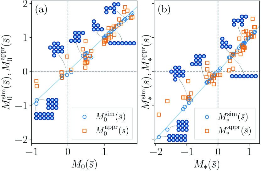
Figure 3: Estimates of the high temperature slope. $M_{0}(\bar{s})$ and $M_{*}(\bar{s})$ correspond to the analytical expressions of Eqs. (5,8). $M_{0}^{\textrm{sim}}(\bar{s})$ and $M_{*}^{\textrm{sim}}(\bar{s})$ are the slopes extracted from a high temperature fit using iterative numerical methods. $M_{0}^{\textrm{appr}}(\bar{s})$ and $M_{*}^{\textrm{appr}}(\bar{s})$ are approximate expressions from Eqs. (6,9).

In Eq. (5), the first term proportional to $\langle n_{ss^{\prime}}\rangle_{\prime}$ accounts for the global slowing down of the dynamics, while the second term proportional to $d_{s}g_{n}(s,\bar{s})$ accounts for the relative energy effect. The global slowing down contribution can be approximated by $\rho_{0}(N)=\langle\langle n_{ss^{\prime}}\rangle_{\prime}\rangle_{s\in{\cal S}}$, which converges exponentially to $\rho_{0}(\infty)\approx 1.64$ for large $N$ (see Supp. Mat. for details). The relative energy effect is dominated by moves from ${\cal B}_{\bar{s}}$ to the target. It is approximately proportional to a measure of cluster compactness defined as the difference in the number of bonds to break between moves leading to and moves not leading to the target $\langle n_{s\bar{s}}-\langle n_{ss^{\prime\prime}}\rangle_{\prime\prime}\rangle_{-}$, where $\langle\,\cdot\,\rangle_{-}=\langle\,\cdot\,\rangle_{s\in{\cal B}_{\bar{s}}}$. This relation is derived and checked in Supp. Mat. We therefore obtain

$$M_{0}^{\mathrm{appr}}({\bar{s}})=\rho_{0}(N)+\rho_{1}\langle n_{s\bar{s}}-\langle n_{ss^{\prime\prime}}\rangle_{\prime\prime}\rangle_{-}\,,$$ (6)

where $\rho_{1}\approx 1.60$. As shown in Fig. 3(a), $M_{0}^{\mathrm{appr}}({\bar{s}})$ provides a fair approximation to $M_{0}({\bar{s}})$. The dispersion originates from assumptions of uncorrelation of $\tau_{\infty}$ with $n_{ss^{\prime}}$, and of variations of $\tau_{\infty}$ dominated by the difference between $\tau_{\infty}(\bar{s},\bar{s})=0$ on the target and $\tau_{\infty}(s,\bar{s})$ in its neighborhood ${\cal B}_{\bar{s}}$. The sign of $M_{0}^{\mathrm{appr}}({\bar{s}})$ can serve as a simple guide to the presence of a minimum as a function of $T$, i.e. an optimal temperature, and also makes explicit the link between the minimum and the compactness of the target. For example, in a linear one-atom-thick target, only the two atoms at the tips can move, so that $\langle n_{s\bar{s}}\rangle_{-}=1$ and an inspection of the possible moves shows that $\langle\langle n_{ss^{\prime\prime}}\rangle_{\prime\prime}\rangle_{-}=4/3$. This leads to $M_{0}^{\mathrm{appr}}({\bar{s}})=\rho_{0}(N)-\rho_{1}/3\approx 0.9>0$ for $N=7$, in agreement with $M_{0}^{\mathrm{sim}}({\bar{s}})\approx 1.04$ found by iterative evaluation. In contrast, in the limit of large compact (square, rectangular, etc) islands, for which $\langle n_{s\bar{s}}\rangle_{-}=1$ and $\langle\langle n_{ss^{\prime\prime}}\rangle_{\prime\prime}\rangle_{-}\rightarrow 3$, we obtain $M_{0}^{\mathrm{appr}}({\bar{s}})=-1.57<0$ leading to a minimum.

Note however that the convergence of value iteration is difficult not only for large clusters, but also for high-energy (i.e., non-compact) target shapes when the temperature is decreased. Indeed, disparate times-scales have to be resolved (fast relaxation towards low-energy shapes vs large time to reach high-energy shapes).

Optimal policy in the presence of forces.

Our goal now is to determine the optimal policy ${\bm{\phi}}_{*}$ that minimizes $\tau_{\bm{\phi}}(s)$, and the resulting optimal first passage time $\tau_{*}(s,\bar{s})=\min_{{\bm{\phi}}}\tau_{{\bm{\phi}}}(s,\bar{s})$ for non-zero forces. Such a problem, called a Markov decision process, can be solved using well-known dynamic programming methods Sutton and Barto (2018); Bellman (2003). We substitute the optimal policy in Eq. (2) to obtain the so-called Bellmann optimality equation

$$\tau_{*}(s,{\bar{s}})=\min_{{\bm{\phi}}(s)}\Bigl{[}t_{\bm{\phi}}(s)+\sum_{s^{\prime}\in{\cal B}_{s}}p_{\bm{\phi}}(s,s^{\prime})\tau_{*}(s^{\prime},{\bar{s}})\Bigr{]}\,.$$ (7)

As in the zero-force case, we iterate Eq.(7). However minimization over the force in $s$ is taken at each iteration. This method, called value iteration, provides both $\tau_{*}(s,{\bar{s}})$ and the optimal policy ${\bm{\phi}}_{*}$. Due to the fast increase of $S_{N}$ with $N$, its computational cost grows exponentially with $N$ (see Supp. Mat.).

We choose a force $\bm{F}$ that is always oriented in $\hat{\bm{x}}$ direction ((10) lattice direction), with 3 possible values: $\{-F_{0}\hat{\bm{x}}$, $\bm{0}$, $F_{0}\hat{\bm{x}}\}$, with $F_{0}>0$. An example of optimal policy is shown in Fig. 1. As an important remark, the force can drive the cluster towards any target shape even if the symmetries of the target are not compatible with those of the force because observation itself (i.e. the knowledge of $s$) breaks the symmetry.

The gain due to the optimal policy is reported in Fig. 4, using the zero-force policy as a reference. In Supp. Mat., we show that using a random-force policy as a reference leads to similar results. As seen from Fig. 4(a), the gain increases not only when $F_{0}$ is increased, but also when $T$ is decreased. This is intuitively expected since the relative change between different rates due to a change of the force increases when $F_{0}/T$ is increased. In addition, the gain increases when the size of the cluster increases, as shown in Fig. 4(b). A naive explanation for this trend is that an increase of $N$ leads to an increase of the number of states $S_{N}$, and therefore to an increase of the number of ways to tune the policy ${\bm{\phi}}$ in order to minimize $\tau_{\bm{\phi}}(s,\bar{s})$.

Again, a high temperature expansion leads to (derivation reported in Supp. Mat.)

$$\tau^{\mathrm{r}}_{*}({\bar{s}}) =\left(1+\frac{M_{*}({\bar{s}})}{T}\right)\tau^{\mathrm{r}}_{\infty}({\bar{s}})\,,$$ (8)

$$M_{*}({\bar{s}}) =M_{0}({\bar{s}})-\frac{F_{0}}{1-S_{N}^{-1}}\Bigl{\langle}\Bigl{|}\tilde{\delta}_{s\bar{s}}\langle u_{ss^{\prime}}\rangle_{\prime}-d_{s}g_{u}(s,{\bar{s}})\Bigr{|}\Bigr{\rangle}_{s\in{\cal S}},$$

where $u_{ss^{\prime}}={\bm{u}_{ss^{\prime}}}\cdot\hat{\bm{x}}$. The numerical solution of Eq. 7 is in agreement with Eq. 8 (up to small deviations due to 4-neighbors particle freezing, see Supp. Mat.).

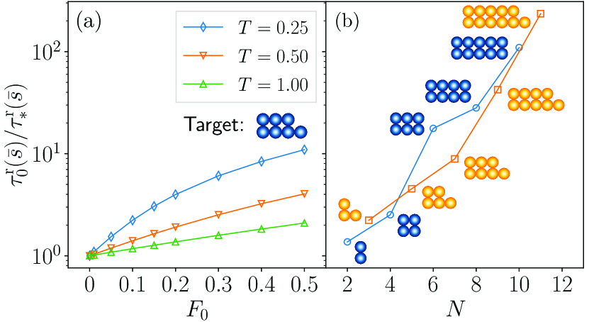
Figure 4: Gain $\tau^{\mathrm{r}}_{0}({\bar{s}})/\tau^{\mathrm{r}}_{*}({\bar{s}})$ in the return time to target due to the optimization of the forces. (a) As a function of the force magnitude $F_{0}$, for a fixed target at different $T$. (b) For similar targets of increasing size, with $T=0.24$ and $F_{0}=0.4$.

Two remarks are in order. First, $\langle u_{ss^{\prime}}\rangle_{\prime}$ is small and its contribution to the term proportional to $F_{0}$ in Eq. (8) is negligible. Second, the absolute value forbids the cancellation of contributions with randomly different signs, leading to a behavior which is qualitatively different from that of $M_{0}(\bar{s})$. Indeed, the average is not dominated by the largest terms coming from the strong change of $\tau_{\infty}(s,{\bar{s}})$ between the target and its first neighbors, but by the typical values of $|d_{s}g_{u}(s,{\bar{s}})|$ in all states. Based on this observation, a detailed analysis reported in Supp. Mat. leads to the approximation

$$M_{*}^{\mathrm{appr}}({\bar{s}})=M_{0}({\bar{s}})-\frac{2^{1/2}}{\pi^{1/2}}F_{0}\;\sigma_{u}\;\sigma_{\tau_{\infty}}\!({\bar{s}})\;\langle d_{s}^{1/2}\rangle_{s\in{\cal S}},$$ (9)

where we have defined the standard deviations

$$\sigma_{u} =\left\langle\left\langle(u_{ss^{\prime}}-\langle u_{ss^{\prime\prime}}\rangle_{\prime\prime})^{2}\right\rangle_{\prime}^{1/2}\right\rangle_{s\in{\cal S}}\,,$$ (10)

$$\sigma_{\tau_{\infty}}({\bar{s}}) =\left\langle\left\langle(\tau_{\infty}(s^{\prime},{\bar{s}})-\langle\tau_{\infty}(s^{\prime\prime},{\bar{s}})\rangle_{\prime\prime})^{2}\right\rangle_{\prime}^{1/2}\right\rangle_{s\in{\cal S}}.$$ (11)

In Fig. 3, the approximation Eq.(9) is seen to be valid up to some dispersion originating mainly in the assumption of uncorrelation between $u_{ss^{\prime}}$ and $\tau_{\infty}$.

While $\langle n_{s\bar{s}}-\langle n_{ss^{\prime\prime}}\rangle_{\prime\prime}\rangle_{-}$ and $\sigma_{u}$ are bounded because $1\leq n_{ss^{\prime}}\leq 4$ and $-1/2\leq-u_{ss^{\prime}}\leq 1/2$, the quantities $\sigma_{\tau_{\infty}}({\bar{s}})$ and $\langle d_{s}^{1/2}\rangle_{s\in{\cal S}}$ grow with $N$ (see Supp. Mat.). Hence, from Eq. (6), $M_{0}^{\mathrm{appr}}(\bar{s})$ is bounded and the contribution proportional to $F_{0}$ in Eq. (9) usually dominates over the term $M_{0}(\bar{s})$ for large $N$. Thus, when $N$ is large enough, $M_{*}(\bar{s})$ should be negative and an optimal temperature should be generically present. This trend is confirmed by Fig. 3(b). Simulations with $N=12$ and $F_{0}=0.4$ (reported in Fig. 10 of Supp. Mat.) also confirm the generic presence of a minimum for larger targets.

Discussion.

For atomic metals clusters where edge diffusion is observed (Ag, Cu, etc.), estimates of the edge diffusion barrier $\sim J$ or kink energies $\sim J/2$ suggest that $J\approx$ 0.2 to 0.3 $\mathrm{eV}$ Ferrando and Tréglia (1994); Yu and Scheffler (1997); Mehl et al. (1999); Nelson et al. (1993); Giesen (2001). For the square 9-atom target depicted in Fig.2 the optimal temperature corresponds to $J/k_{B}T\approx 2$. Choosing $J=0.2\,$\mathrm{eV}$$ we obtain an optimal temperature $\approx 10^{3}$ K which is too high to be observed in usual experiments. Thus, $\tau_{0}(s,\bar{s})$ should decrease with temperature in usual experimental conditions. If needed, a quench can also be used to freeze the cluster once the target shape is reached. However, using electromigration as an external force leads to Tao et al. (2010) $F_{0}a/J\approx 10^{-4}$, which is too small to allow for the control of few-atoms clusters.

Edge diffusion can also be observed with colloids Hubartt and Amar (2015). Using colloids with depletants, $J\sim$ few $k_{B}T$ Nozawa et al. (2018). The optimal temperature should then be observable in the absence of force. Thermophoretic forces Helden et al. (2015); Braibanti et al. (2008); Würger (2010) for polystyrene beads of radius $2.5\,$\mathrm{\SIUnitSymbolMicro m}$$ are $\sim 10\,k_{B}T/$\mathrm{\SIUnitSymbolMicro m}$$ Helden et al. (2015). Hence, micron-size colloids can lead to $F_{0}a/J\sim 1$, which allows for shape control by a macroscopic force.

However, most experiments on colloid clusters report mass transport dominated by attachment-detachment at the edges Ganapathy et al. (2010). Our analysis can be adapted to vacancy clusters Martínez-Galera et al. (2014); García et al. (2007); Pariente et al. (2020) with volume-preserving detachment-diffusion-reattachment events. Moreover, other two or three-dimensional lattices also could be analyzed. Furthermore, multi-particle and off-lattice processes (such as those involved in dislocation-mediated dynamics) can be included as long as they are pre-determined (using e.g. energy-exploration methods) and their number is finite, to allow for the numerical solution of Eqs. 2 and 7. Since the presence of the minimum depends only on the generic competition between the relative energy effect and global slowing down, we speculate that it should not depend on the details of mass transport kinetics.

In conclusion, thermal fluctuations can be used to reach desired nano-cluster shapes. There is a temperature that minimizes the time to reach large-enough and compact shapes. Furthermore, macroscopic fields can help gaining orders of magnitude in the time to reach arbitrary shapes. We hope that our work will motivate experimental investigations for the control of atomic and colloidal clusters, and will open theoretical directions for the optimization of first passage times on graphs.

References

- Binnig and Rohrer (1983) G. Binnig and H. Rohrer, Surf. Sci. 126, 236 (1983).
- Eigler and Schweizer (1990) D. M. Eigler and E. K. Schweizer, Nature 344, 524 (1990).
- Cooper et al. (2018) A. Cooper, J. P. Covey, I. S. Madjarov, S. G. Porsev, M. S. Safronova, and M. Endres, Phys. Rev. X 8, 041055 (2018).
- Barredo et al. (2016) D. Barredo, S. de Léséleuc, V. Lienhard, T. Lahaye, and A. Browaeys, Science 354, 1021 (2016).
- Martínez-Galera et al. (2014) A. Martínez-Galera, I. Brihuega, A. Gutiérrez-Rubio, T. Stauber, and J. Gómez-Rodríguez, Sci. Rep. 4, 1 (2014).
- Erickson et al. (2011) D. Erickson, X. Serey, Y.-F. Chen, and S. Mandal, Lab Chip 11, 995 (2011).
- Junno et al. (1995) T. Junno, K. Deppert, L. Montelius, and L. Samuelson, Appl. Phys. Lett. 66, 3627 (1995).
- Baur et al. (1998) C. Baur, A. Bugacov, B. E. Koel, A. Madhukar, N. Montoya, T. R. Ramachandran, A. A. G. Requicha, R. Resch, and P. Will, Nanotechnology 9, 360 (1998).
- Rubio-Sierra et al. (2005) F. J. Rubio-Sierra, W. M. Heckl, and R. W. Stark, Adv. Eng. Mater. 7, 193 (2005).
- Korda et al. (2002) P. T. Korda, M. B. Taylor, and D. G. Grier, Phys. Rev. Lett. 89, 128301 (2002).
- Grier (2003) D. G. Grier, Nature 424, 810 (2003).
- McCormack et al. (2018) P. McCormack, F. Han, and Z. Yan, J. Phys. Chem. Lett. 9, 545 (2018).
- Kuhn et al. (2005) P. Kuhn, J. Krug, F. Hausser, and A. Voigt, Phys. Rev. Lett. 94, 166105 (2005).
- Mahadevan and Bradley (1999) M. Mahadevan and R. M. Bradley, Phys. Rev. B 59, 11037 (1999).
- Pierre-Louis and Einstein (2000) O. Pierre-Louis and T. L. Einstein, Phys. Rev. B 62, 13697 (2000).
- Curiotto et al. (2019) S. Curiotto, F. Leroy, P. Müller, F. Cheynis, M. Michailov, A. El-Barraj, and B. Ranguelov, J. Cryst. Growth 520, 42 (2019).
- Khare et al. (1995) S. V. Khare, N. C. Bartelt, and T. L. Einstein, Phys. Rev. Lett. 75, 2148 (1995).
- Lai et al. (2017) K. C. Lai, D.-J. Liu, and J. W. Evans, Phys. Rev. B 96, 235406 (2017).
- Juárez and Bevan (2012) J. J. Juárez and M. A. Bevan, Adv. Funct. Mater. 22, 3833 (2012).
- Juárez et al. (2012) J. J. Juárez, P. P. Mathai, J. A. Liddle, and M. A. Bevan, Lab Chip 12, 4063 (2012).
- Xue et al. (2014) Y. Xue, D. J. Beltran-Villegas, X. Tang, M. A. Bevan, and M. A. Grover, IEEE Trans. Control Syst. Technol. 22, 1956 (2014).
- Sutton and Barto (2018) R. S. Sutton and A. G. Barto, Reinforcement Learning: An Introduction, 2nd ed. (The MIT Press, 2018).
- Bellman (2003) R. E. Bellman, Dynamic Programming (Dover Publications, Inc., USA, 2003).
- Giesen (2001) M. Giesen, Prog. Surf. Sci. 68, 1 (2001).
- Tao et al. (2010) C. Tao, W. G. Cullen, and E. D. Williams, Science 328, 736 (2010).
- Hubartt and Amar (2015) B. C. Hubartt and J. G. Amar, J. Chem. Phys. 142, 024709 (2015).
- Plass et al. (2001) R. Plass, J. A. Last, N. Bartelt, and G. Kellogg, Nature 412, 875 (2001).
- Heinonen et al. (1999) J. Heinonen, I. Koponen, J. Merikoski, and T. Ala-Nissila, Phys. Rev. Lett. 82, 2733 (1999).
- Leroy et al. (2020) F. Leroy, A. El Barraj, F. Cheynis, P. Müller, and S. Curiotto, Phys. Rev. B 102, 235412 (2020).
- VanSaders and Glotzer (2021) B. VanSaders and S. C. Glotzer, Proc. Natl. Acad. Sci. U.S.A 118, e2017377118 (2021).
- Huang et al. (2018) R. Huang, Y. Wen, A. F. Voter, and D. Perez, Phys. Rev. Materials 2, 126002 (2018).
- Trushin et al. (2001) O. Trushin, P. Salo, M. Alatalo, and T. Ala-Nissila, Surf. Sci. 482-485, 365 (2001).
- Glasstone et al. (1941) S. Glasstone, K. J. Laidler, and H. Eyring, The Theory of Rate Processes: The Kinetics of Chemical Reactions, Viscosity, Diffusion and Electrochemical Phenomena, International chemical series (McGraw-Hill Book Company, Inc., 1941).
- Liu and Weeks (1998) D.-J. Liu and J. D. Weeks, Phys. Rev. B 57, 14891 (1998).
- Sanchez and Evans (1999) J. R. Sanchez and J. W. Evans, Phys. Rev. B 59, 3224 (1999).
- Combe and Larralde (2000) N. Combe and H. Larralde, Phys. Rev. B 62, 16074 (2000).
- Van Kampen (1992) N. G. Van Kampen, Stochastic processes in physics and chemistry (Elsevier, 1992).
- Note (1) As a technical remark, this definition requires to extend the policy and define a force on the target state itself. However, due to the Markovian character of the dynamics, this does not affect the mean first passage time to target and the optimal policy in the other states outside the target.
- Dougherty et al. (2002) D. B. Dougherty, I. Lyubinetsky, E. D. Williams, M. Constantin, C. Dasgupta, and S. D. Sarma, Phys. Rev. Lett. 89, 136102 (2002).
- Constantin et al. (2003) M. Constantin, S. Das Sarma, C. Dasgupta, O. Bondarchuk, D. B. Dougherty, and E. D. Williams, Phys. Rev. Lett. 91, 086103 (2003).
- Guttmann (2009) A. J. Guttmann, Polygons, Polyominoes and Polycubes, Lecture Notes in Physics 775 (Springer, 2009).
- Jensen and Guttmann (2000) I. Jensen and A. J. Guttmann, J. Phys. A Math. Theor. 33, L257 (2000).
- Lovász (1993) L. Lovász, Combinatorics, Paul Erdős is eighty 2, 1 (1993).
- Lin et al. (2012) Y. Lin, A. Julaiti, and Z. Zhang, J. Chem. Phys. 137, 124104 (2012).
- Tejedor et al. (2009) V. Tejedor, O. Bénichou, and R. Voituriez, Phys. Rev. E 80, 065104 (2009).
- Baronchelli and Loreto (2006) A. Baronchelli and V. Loreto, Phys. Rev. E 73, 026103 (2006).
- Noh and Rieger (2004) J. D. Noh and H. Rieger, Phys. Rev. Lett. 92, 118701 (2004).
- Ferrando and Tréglia (1994) R. Ferrando and G. Tréglia, Phys. Rev. B 50, 12104 (1994).
- Yu and Scheffler (1997) B. D. Yu and M. Scheffler, Phys. Rev. B 55, 13916 (1997).
- Mehl et al. (1999) H. Mehl, O. Biham, I. Furman, and M. Karimi, Phys. Rev. B 60, 2106 (1999).
- Nelson et al. (1993) R. Nelson, T. Einstein, S. Khare, and P. Rous, Surf. Sci. 295, 462 (1993).
- Nozawa et al. (2018) J. Nozawa, S. Uda, S. Guo, A. Toyotama, J. Yamanaka, N. Ihara, and J. Okada, Cryst. Growth Des. 18, 6078 (2018).
- Helden et al. (2015) L. Helden, R. Eichhorn, and C. Bechinger, Soft Matter 11, 2379 (2015).
- Braibanti et al. (2008) M. Braibanti, D. Vigolo, and R. Piazza, Phys. Rev. Lett. 100 (2008).
- Würger (2010) A. Würger, Rep. Prog. Phys. 73, 126601 (2010).
- Ganapathy et al. (2010) R. Ganapathy, M. R. Buckley, S. J. Gerbode, and I. Cohen, Science 327, 445 (2010).
- García et al. (2007) P. García, R. Sapienza, A. Blanco, and C. López, Adv. Mater. 19, 2597 (2007).
- Pariente et al. (2020) J. A. Pariente, N. Caselli, C. Pecharromán, A. Blanco, and C. López, Small 16, 2002735 (2020).