Construction and local equivalence of dual-unitary operators: from dynamical maps to quantum combinatorial designs

Abstract

While quantum circuits built from two-particle dual-unitary (maximally entangled) operators serve as minimal models of typically nonintegrable many-body systems, the construction and characterization of dual-unitary operators themselves are only partially understood. A nonlinear map on the space of unitary operators was proposed in PRL. 125, 070501 (2020) that results in operators being arbitrarily close to dual unitaries. Here we study the map analytically for the two-qubit case describing the basins of attraction, fixed points, and rates of approach to dual unitaries. A subset of dual-unitary operators having maximum entangling power are 2-unitary operators or perfect tensors, and are equivalent to four-party absolutely maximally entangled states. It is known that they only exist if the local dimension is larger than $d=2$. We use the nonlinear map, and introduce stochastic variants of it, to construct explicit examples of new dual and 2-unitary operators. A necessary criterion for their local unitary equivalence to distinguish classes is also introduced and used to display various concrete results and a conjecture in $d=3$. It is known that orthogonal Latin squares provide a “classical combinatorial design” for constructing permutations that are 2-unitary. We extend the underlying design from classical to genuine quantum ones for general dual-unitary operators and give an example of what might be the smallest sized genuinely quantum design of a 2-unitary in $d=4$.

I Introduction

In recent years a major research trend uses tools of quantum information theory to understand the puzzles of quantum many-body physics. The typically complex entanglement structure of many-body states drives cross fertilization across various fields of research in physics. Particularly, in the areas of condensed matter physics and string theory, quantum information theory continues to play an exciting role in creating new avenues of understanding Amico et al. (2008); Zeng et al. (2015); Jahn and Eisert (2021); Kibe et al. (2022).

Quantum computers allow the realization of the vision of Feynman Feynman (1982) on the efficient simulation of physical systems Georgescu et al. (2014). In the present era of Noisy-Intermediate-Scale-Quantum (NISQ) Preskill (2018) computing such simulations become realistic Ippoliti et al. (2021). The universality of quantum computing allows simulation of any quantum system, where quantum circuits are built using unitary operators or gates acting on single particle and two particle subsystems. A quantum computer is itself a controllable quantum many-body system. Traditional approaches involve studying the properties of systems based on the Hamiltonian evolution and spectra. At this juncture it is important to understand properties of quantum many-body systems from the quantum circuit formalism and to contrast that with the traditional studies.

Quantum advantage using random unitary circuits has been explored in recent experiments using Google’s “sycamore” processor Arute et al. (2019) and “Zuchongzhi 2.0” Zhu et al. (2022). Similar models are used in studies of entanglement evolution in many-body quantum systems in which the random unitary gates act on nearest neighbours Nahum et al. (2018, 2017); Khemani et al. (2018); von Keyserlingk et al. (2018); Chan et al. (2018). Quantum circuits, in arbitrary local dimensions, without any random interactions have been proposed as elegant minimal models that can span the gamut of integrable to fully chaotic quantum many-body systems Akila et al. (2016); Bertini et al. (2019a); Gutkin et al. (2020); Braun et al. (2020). These quantum circuits have a special “duality” property that the evolution operator in the spatial as well as in the temporal direction of the circuit are governed by unitary dynamics. The origin of this duality lies in the two-particle unitary gates being dual-unitary Bertini et al. (2019a). This duality facilitates an analytical treatment of many quantities such as two-point correlation functions, spectral form-factor, operator entanglement, out-of-time-order correlators and the exact study the entanglement dynamics Bertini et al. (2018, 2019a, 2019b); Gutkin et al. (2020); Bertini et al. (2020a); Kos et al. (2021); Lerose et al. (2021); Garratt and Chalker (2021); Flack et al. (2020); Bertini et al. (2020b); Piroli et al. (2020); Claeys and Lamacraft (2020); Klobas et al. (2021); Ippoliti et al. (2022); Ippoliti and Khemani (2021); Klobas and Bertini (2021); Claeys and Lamacraft (2022); Zhou and Harrow (2022). The two-particle unitary from which the circuit is built, plays a significant role in the following and is an operator in $d^{2}$ dimensional space where the local dimension is $d$ and is typically denoted as $U$.

On the other hand entanglement of unitary operators, similar to states, has been studied from the early days of quantum information theoryZanardi et al. (2000); Zanardi (2001); Wang and Zanardi (2002); Wang et al. (2003); Nielsen et al. (2003); Vidal and Cirac (2002); Hammerer et al. (2002); Collins et al. (2001); Eisert et al. (2000); Cirac et al. (2001). Quantities such as operator entanglement Zanardi (2001), entangling power Zanardi et al. (2000) and complexity of an operator Nielsen et al. (2006) are few measures that quantify the nonlocal properties of unitary operators. Operator entanglement measures how entangled an operator is when viewed as a vector in a product vector space. It has been identified that an unitary operator is dual-unitary if and only if it has maximum possible operator entanglement Rather et al. (2020). Entangling power quantifies the average entanglement produced by a bipartite unitary operator acting on an ensemble of pure product states. A special subclass of dual-unitary operators are those having the maximum possible entangling power allowed by local dimensions. These are the same operators that have been referred to variously as 2-unitary Goyeneche et al. (2015) or perfect tensors Pastawski et al. (2015).

The exactly calculable two-point correlation functions in dual-unitary circuits enable the characterization of the many-body system in terms of an ergodic hierarchy, from ergodic to Bernoulli through mixing Bertini et al. (2019a); Aravinda et al. (2021). It is identified that the dual-unitary circuit is Bernoulli, when correlations instantly decay, if and only if the two-particle unitary operator has maximum entangling power Aravinda et al. (2021). Additionally, a sufficient condition for the many-body circuit to show the mixing behavior is derived as a function of entangling power Aravinda et al. (2021). These results establish a close connection between the entangling properties of two particle unitary operators from which the many-body quantum circuits are built and the dynamical nature of the many-body systems.

Let a bipartite pure quantum state’s Schmidt form be $\ket{\psi}_{AB}=\sum_{i=0}^{d-1}\sqrt{\lambda_{i}}\ket{ii}/\sqrt{d}$, where $d$ is the local Hilbert space dimension. Setting $\lambda_{i}=1\;\text{for all}\;i$ in this expansion results in $\ket{\Phi}=\sum_{i=1}^{d}\ket{ii}/\sqrt{d}$ which is a maximally entangled state, in fact the one that is closest to $\ket{\psi_{AB}}$. Any set of orthonormal bases in the subspaces constructs such maximally entangled states.

In contrast the construction of maximally entangled unitary operators do not follow from orthonormal operator bases. Express an unitary operator in operator Schmidt form, $U=\sum_{j=1}^{d^{2}}\sqrt{\lambda_{j}}X_{j}\otimes Y_{j}$, $\tr(X_{j}^{\dagger}X_{k})=\tr(Y_{j}^{\dagger}Y_{k})=\delta_{jk}$ and $\lambda_{j}\geq 0$. $U$ is maximally entangled or dual-unitary iff $\lambda_{i}=1\;\text{for all}\;i$. However the constraint of unitarity is stronger than the constraint of normalization on the state and this imposes complex conditions on the Schmidt matrices $X_{j}$ and $Y_{j}$. Thus simply assigning $\lambda_{i}=1\;\text{for all}\;i$ does not retain unitarity although it does result in a maximally entangled operator. This makes it hard to analytically construct dual-unitary operators. Construction of maximally entangled unitaries was discussed at least as early as in Ref. Tyson (2003a).

If the local dimension is $d=2$, namely for qubits, all possible dual-unitary operators can be parametrized using the Cartan decomposition Bertini et al. (2019a). There are no 2-unitary or perfect tensors in this case. While a complete parametrization of dual-unitary operators for $d>2$ is not known, many classes and examples have been examined and used thus far. The swap or flip operator is a simple example of a dual-unitary operator. The discrete Fourier transform in $d^{2}$ dimensions maximizes operator entanglement Tyson (2003b); Jonnadula et al. (2020) and is hence also a dual-unitary. However, the swap has zero entangling power, while the Fourier transform has a finite value. Diagonal and block diagonal operators, along with the swap gate can be used to construct dual-unitary operator Claeys and Lamacraft (2021); Aravinda et al. (2021). These have limited entangling power and in partcular cannot reach the maximum value Aravinda et al. (2021). The dual-unitary operators introduced recently in Ref. Singh and Nechita (2022) are also bounded by the entangling power of diagonal unitary operators.

A numerical iterative algorithm which produces unitary operators arbitrarily close to being dual-unitary has been presented in Rather et al. (2020). This algorithm can yield dual-unitary operators with a wide range of entangling powers, especially exceeding the bound corresponding to block-diagonal based constructions. Remarkably, the numerical algorithm can also yield exact analytical forms for dual-unitary operators Aravinda et al. (2021) and several other examples, including new 2-unitaries, are displayed further below. A slightly modified algorithm has been used to positively settle an open problem on the existence of four-party absolutely maximally entangled (AME) states of local dimension six Rather et al. (2022), see also Ref. Życzkowski et al. (2022) for an elaborate discussion of the solution. AME states are genuinely entangled multipartite pure states which have maximal entanglement in all bipartitions Helwig et al. (2012). Thus an AME state of $N$ qudits each of dimesion $d$ denoted as AME($N,d$) has all subsystems of size $\lfloor N/2\rfloor$ maximally mixed.

The numerical algorithm acts generically as a dynamical map in the space of unitary operators. These are thus high dimensional dynamical systems which deserve to be studied in their own right. In this work, we study the fixed point structure of the map. In particular for the case of two qubits, an explicit analytical form of the map is derived. This enables deriving dynamical characteristics such as the rate of approach to attractors which are dual-unitary operators. A variety of dynamical behaviours have been observed: (i) power-law approaches to the swap gate, (ii) exponential approach to other dual unitary gates, with a rate that diverges for the maximally entangling case of the dcnot gate.

Due to operator-state isomorphism, a 2-unitary operator is equivalent to a four-party AME state Goyeneche et al. (2015). There are various ways of constructing AME states in which quantum combinatorial designs are used Goyeneche et al. (2015, 2018). Since 2-unitaries are a subset of dual unitaries, a less restrictive combinatorial design underlying dual-unitary operators that are permutations was found in Aravinda et al. (2021). In this work, we extend such combinatorial designs to dual-unitary operators going beyond permutations. We define stochastic dynamical maps capable of generating such structured dual-unitary operators.

Apart from dual-unitary operators, the maps presented in Rather et al. (2020) can be used to generate infinitely many 2-unitaries for $d>2$. An important question now arises if the 2-unitaries so obtained are local unitarily (LU) equivalent to each other and to 2-unitary permutations of the same size. Two bipartite unitary operators $U$ and $U^{\prime}$ on $\mathcal{H}_{d}\otimes\mathcal{H}_{d}$ are said to local unitarily equivalent, denoted $U\overset{\text{LU}}{\sim}U^{\prime}$, if there exist single qudit unitary gates $u_{1},u_{2},v_{1},v_{2}$ such that

$$U^{\prime}=(u_{1}\otimes u_{2})U(v_{1}\otimes v_{2}).$$ (1)

However, as far as we know, there is no general procedure to identify LU equivalent unitary operators, apart from the case of two-qubits Cirac et al. (2001). This problem becomes acute when the operators concerned have the same entangling powers, such as the 2-unitaries. In this work, we address this question by proposing a necessary criterion for LU equivalence between bipartite unitary operators that can potentially work also in the case of 2-unitaries.

This leads us to conjecture that all two-qutrit 2-unitaries are LU equivalent to each other. From an exhaustive search, we find that the special subset of $72$ possible 2-unitary permutations of size 9 are LU equivalent to each other. For local Hilbert space dimension $d=4$, we find that this still continues to hold: indeed there are $6912$ 2-unitary permutations, and we find that these can generated from any one of them by local permuations. Thus upto LU equivalence, we find that there is only one 2-unitary permutation in $d=3,4$ and implies that there is only one unique orthogonal Latin square of size $3$ and $4$. Note that the connection between 2-unitary permutations and orthogonal Latin squares has been known for some time Clarisse et al. (2005).

Although there is only one 2-unitary permutation upto LU equivalence, further below, we give an explicit example of a 2-unitary of size 16 which is not LU equivalent to any 2-unitary permutation of the same size. In other words, we give an explicit example of an AME state of four ququads which is not LU connected to an AME state of four ququads with minimal support. Minimal support four-party AME states have $d^{2}$ nonvanishing coefficients in some product orthonormal basis, which is the smallest number possible Goyeneche et al. (2015). These new examples of AME states can be used to construct new error-correcting codes as was done in Rather et al. (2022) and can provide insights about the most general underlying combinatorial designs 2-unitaries possess. For $d=5$ we show that there are two LU inequivalent 2-unitary permutations or equivalently, two LU inequivalent AME states of minimal support. This contradicts Conjecture 2 in Ref. Burchardt and Raissi (2020) which implies that all four party AME states of minimal support are LU equivalent for all local dimensions $d$.

I.1 Summary of principal results and structure of the paper

In view of the length of this paper, we summarize some of the main results here.

1. Dynamical maps for generation of dual-unitary operators, Sections  (III, IV)

   1. It is shown in Proposition 18 that the map preserves local unitary equivalence.

   2. Explicit form of the map for the two-qubit case is derived. This is used to show that all dual unitaries are period-two points, and conversely all period-two points are dual unitaries. It is shown that convergence of the map to dual unitaries is typically exponential.

2. Quantum designs and new classes of 2-unitaries and AME states, Sec.  (V– (VII)

   1. A necessary criterion for LU equivalence between bipartite unitary gates is proposed, and is particularly useful for establishing inequivalence between 2-unitary operators and AME states.

   2. An AME state of four qudits each of local dimension 4, AME$(4,4)$, is constructed such that it is not LU equivalent to any known AME state obtained from classical orthogonal Latin squares. It is likely to be the simplest genuine orthogonal quantum Latin square construction.

   3. For local dimensions $d=3,$ and $d=4$, it is shown that there is only one LU class of AME states constructed from orthogonal Latin squares (OLS). However, we show that there are more than one such LU class for $d>4$.

The paper is structured as follows. In Sec. (II), the basic terminologies used in the current work is defined. In Sec.  (III), the non-linear iterative maps from which dual-unitary and 2-unitary operators are produced is described, and their fixed point structure is discussed. Stochastic generalizations are introduced to result in specially structured operators. In Sec. (IV) the iterative map is studied in explicit forms for the case of qubits. Here we analytically estimate the power-law or exponential approach to dual-unitary operators. In Sec (V) combinatorial designs corresponding to dual-unitary operators is discussed. In Sec.  (VI) the question of local unitary equivalence of 2-unitary operators is discussed, specially for the small cases of $d=3$, and $4$. In Sec. (VII) permutations small dimensions is studied in detail via their entangling powers and gate-typicality. Classification of LU classes for dual-unitary and T-dual unitary permutation operators is given for $d=2,3$. Finally we conclude in Sec. (VIII).

II Preliminaries and definitions

In this section, we mostly recall some relevant quantities and measures.

II.1 Operator entanglement and entangling power

Any operator $X\in\mathcal{B}(\mathcal{H}_{d})$ is mapped to the state $\ket{X}\in\mathcal{H}_{d}\otimes\mathcal{H}_{d}$ as

$$\ket{X}:=(X\otimes I)\ket{\Phi},$$ (2)

where $\{\ket{i}\}_{i=1}^{d}$ is an orthonormal basis in $\mathcal{H}_{d}$ and $\ket{\Phi}:=\frac{1}{\sqrt{d}}\sum_{i=1}^{d}\ket{ii}$ is the generalized Bell state. A bipartite unitary operator $U=\sum_{ij}^{d^{2}}\alpha_{ij}e_{i}^{A}\otimes e_{j}^{B}\in\mathcal{B}(\mathcal{H}_{d}\otimes\mathcal{H}_{d})$, is mapped to $\ket{U}=\sum_{ij}^{d^{2}}\alpha_{ij}\ket{e_{i}}_{A}\otimes\ket{e_{j}}_{B}\in\mathcal{H}_{d^{2}}\otimes\mathcal{H}_{d^{2}}$, where $e^{A,B}_{i}$ are a pair of operator bases in $\mathcal{B}(\mathcal{H}_{d})$.

The entanglement of an unitary operator $U$ is the entanglement of the state $\ket{U}=\sum_{j=1}^{d^{2}}\sqrt{\lambda_{j}}\ket{X^{A}_{j}}\ket{Y^{B}_{j}}$. The Schmidt decomposition of $U$ is given by

$$U=\sum_{j=1}^{d^{2}}\sqrt{\lambda_{j}}X_{j}^{A}\otimes Y_{j}^{B},$$ (3)

with $\tr{{X_{j}^{A}}^{\dagger}X_{k}^{A}}=\tr{{Y_{j}^{B}}^{\dagger}Y_{k}^{B}}=\delta_{jk},\quad\sum_{j=1}^{d^{2}}\lambda_{j}=d^{2}$. The operator entanglement of $U$ is defined in terms of linear entropy as

$$E(U)=1-\frac{1}{d^{4}}\sum_{j=1}^{d^{2}}\lambda_{j}^{2},$$ (4)

where $0\leq E(U)\leq 1-1/d^{2}$.

Another related, but distinct, entanglement facet of an unitary operator $U$ is its entangling power, $e_{p}(U)$. It is defined as the average entanglement produced due to its action on pure product states distributed according to the uniform, Haar measure,

$$e_{p}(U)=C_{d}\overline{\mathcal{E}(U\ket{\phi_{1}}\otimes\ket{\phi_{2}})}^{\ket{\phi_{1}},\ket{\phi_{2}}},$$ (5)

where $\mathcal{E}(\cdot)$ can be any entanglement measure, and $C_{d}$ is a constant scale factor. Considering $\mathcal{E}(\cdot)$ to be the linear entropy, the entangling power can be directly calculated using operator entanglement Zanardi (2001) as follows. Let $S$ be the swap operator such that

$$S\ket{\phi_{A}}\ket{\phi_{B}}=\ket{\phi_{B}}\ket{\phi_{A}},$$ (6)

for all $\ket{\phi_{A}}\in\mathcal{H}_{d},\,\ket{\phi_{B}}\in\mathcal{H}_{d}$. We choose $C_{d}$ such that the scaled entangling power $0\leq e_{p}(U)\leq 1$ is given by

$$e_{p}(U)=\frac{1}{E(S)}[E(U)+E(US)-E(S)],$$ (7)

where $E(S)=1-1/d^{2}$.

Note that the swap operator is such that it has the maximum possible operator entanglement, however the entangling power $e_{p}(S)=0$. For any operator $U$, $e_{p}(U)=e_{p}(US)=e_{p}(SU)$. The so-called gate-typicality $g_{t}(U)$ Jonnadula et al. (2017) distinguishes these and is defined as

$$g_{t}(U)=\frac{1}{2E(S)}[E(U)-E(US)+E(S)],$$ (8)

and also ranges from $0$ to $1$, with $g_{t}(S)=1$ and vanishes for all local gates.

II.2 Matrix reshaping

A bipartite unitary operator $U$ on $\mathcal{H}_{d}\otimes\mathcal{H}_{d}$ can be expanded in product basis as

$$U=\sum_{i\alpha j\beta}\matrixelement{i\alpha}{U}{j\beta}\ket{i\alpha}\bra{j\beta}$$ (9)

There are four basic matrix rearrangements of $U$ that we use in this work :

1. Realignment operations:

   $$\quad R_{1}:\matrixelement{i\alpha}{U}{j\beta} =\matrixelement{\beta\alpha}{U^{R_{1}}}{ji}$$ (10)

   $$\quad R_{2}:\matrixelement{i\alpha}{U}{j\beta} =\matrixelement{ij}{U^{R_{2}}}{\alpha\beta}$$ (11)

2. Partial Transpose operations:

   $$\quad\Gamma_{1}:\matrixelement{i\alpha}{U}{j\beta} =\matrixelement{j\alpha}{U^{\Gamma_{1}}}{i\beta}$$ (12)

   $$\quad\Gamma_{2}:\matrixelement{i\alpha}{U}{j\beta} =\matrixelement{i\beta}{U^{\Gamma_{2}}}{j\alpha}$$ (13)

The relation between entanglement and matrix reshapings becomes clear on considering the state $\ket{U}$ as now a 4-party state $\ket{\psi}\in\mathcal{H}_{d}\otimes\mathcal{H}_{d}\otimes\mathcal{H}_{d}\otimes\mathcal{H}_{d}$:

$$\ket{\psi}_{ABCD}=(U_{AB}\otimes I_{CD})\ket{\Phi}_{AC}\ket{\Phi}_{BD},$$ (14)

where $\ket{\Phi}=\frac{1}{\sqrt{d}}\sum_{i}^{d}\ket{ii}$ is the generalized Bell state. The reduced state corresponding to the three possible partition $AB|CD$, $AC|BD$ and $AD|BC$ are given by

$$\rho_{AB}=\frac{1}{d^{2}}UU^{\dagger},\,\rho_{AC}=\frac{1}{d^{2}}U^{R_{2}}U^{R_{2}\dagger},\,\rho_{AD}=\frac{1}{d^{2}}U^{\Gamma_{2}}U^{\Gamma_{2}\dagger}.$$ (15)

Using $(X\otimes Y)^{R_{2}}=\outerproduct{X}{Y^{*}}$, where * refers to complex conjugation in the computational basis. It is easy to see $U^{R_{2}}U^{R_{2}\dagger}=\sum_{1}^{d^{2}}\lambda_{j}\outerproduct{X_{j}}{X_{j}}$. The Schmidt value $\lambda_{j}$ are the singular values of $U^{R_{2}}$ (which are the same as the singular values of $U^{R_{1}}$). The operator entanglement $E(U)$ can be interpreted as the linear entropy of entanglement of the bipartition $AC|BD$, and can be expressed in terms of $U^{R}$ as

$$E(U)=1-\frac{1}{d^{4}}\Tr{(U^{R}U^{R\dagger})^{2}}.$$ (16)

Similarly, the operator entanglement $E(US)$ is the linear entropy of the bipartition $AD|BC$ and is

$$E(US)=1-\frac{1}{d^{4}}\text{Tr}{(U^{\Gamma}U^{\Gamma\dagger})^{2}}.$$ (17)

Whenever the subscripts on $R$ and $\Gamma$ have been dropped they can refer equally to either of the two operations. Note that the singular values of $U^{R}$ and $U^{\Gamma}$ are all local unitary invariants (LUI).

We recall definitions of some special families of unitary operators and also introduce some new families of unitary operators.

Definition 1 (Dual unitary Bertini et al. (2019a)).

If the realigned matrix $U^{R}$ of unitary operator $U$ is also unitary, then $U$ is called a dual unitary.

Definition 2 (T-dual unitary Aravinda et al. (2021)).

If the partial transposed matrix $U^{\Gamma}$ of a unitary operator $U$ is also unitary, then $U$ is called a T-dual unitary.

Definition 3 (2-unitary Goyeneche et al. (2015)).

A unitary $U$ for which both $U^{R}$ and $U^{\Gamma}$ are also unitary is called 2-unitary.

Definition 4 (Self dual unitary).

Unitary operator $U$ for which $U^{R}=U$ is called a self-dual unitary.

Note that for a 2-unitary $E(U)=E(US)=E(S)=1-1/d^{2}$ are maximized and thus from Eq. (7) $e_{p}(U)=1$, the maximum possible value. Thus the corresponding four-party state given by Eq. (14) is maximally entangled along all three bipartitions and is an absolutely maximally entangled state of four qudits; AME($4,d$).

In the mathematics literature, the class of unitary operators which remain unitary under ‘block-transpose’ have been studied since 1989 Ocneanu (1988); Krishnan and Sunder (1996); Jones ; Reutter and Vicary (2019); Benoist and Nechita (2017a); Kodiyalam et al. (2020); Nechita et al. (2021) . Referred to as biunitaries, they are dual unitary upto multiplication by swap, and is the result of the $\Gamma_{1}$ operation above. However, the term “biunitary” seems to be used interchangably for both dual and T-dual unitary operators and subsequently no special studies of 2-unitaries, that are both dual and T-dual seems to exist.

T-dual and dual unitary have very different entanglement properties, as reflected in their two most prominent representatives: the identity and the swap gate. However, they are related in the sense that every T-dual unitary $U$ has a dual partner $US$ (or $SU$). Note that if $U$ is 2-unitary, so also are $U^{R}$ and $U^{\Gamma}$. For example, the realignment of $U^{R}$ is $U$ itself, while $(U^{R})^{\Gamma}=U^{\Gamma}S$, which is evidently unitary given that $U$ is 2-unitary.

III Dual-unitary and 2-unitary operators from nonlinear iterative maps

Complete parametrization of dual unitary operators for arbitrary local Hilbert space dimension $d$ is not known in general except in the two-qubit case Bertini et al. (2019a). Several (incomplete) analytic constructions of families of dual unitary operators have been proposed based on complex Hadamard matrices Gutkin and Osipov (2016), diagonal Claeys and Lamacraft (2021), and block-diagonal unitary matrices Aravinda et al. (2021). Here we briefly review the non-linear maps introduced in Rather et al. (2020) to generate unitary operators which are arbitrarily close to dual unitaries.

III.1 Dynamical map for dual unitaries

The following map is defined on the space of bipartite unitary operators,

$$\mathcal{M}_{R}:\mathcal{U}(d^{2})\longrightarrow\mathcal{U}(d^{2}).$$

One complete action of $\mathcal{M}_{R}$ on a seed unitary $U_{0}$ consists of the following two steps:

1. Linear part: Realignment of $U_{0}$: $U_{0}\xrightarrow{R}U_{0}^{R}$,

2. Non-linear part: Projection of $U_{0}^{R}$ to the nearest unitary matrix $U_{1}$ given by its polar decomposition (PD) Fan and Hoffman (1955); Keller (1975); $U_{0}^{R}=U_{1}\sqrt{U_{0}^{R\,\dagger}U_{0}^{R}}$.

Note that $U_{0}^{R}$ must be of full rank for the map to be well defined as the polar decomposition of rank deficient matrices is not uniquely defined. We write one complete action of the map on $U_{0}$ as

$$\mathcal{M}_{R}[U_{0}]:=U_{1}.$$

After $n$ iterations,

$$\underbrace{\mathcal{M}_{R}\circ\mathcal{M}_{R}\circ\cdots\circ\mathcal{M}_{R}}_{n\;\text{times}}[U_{0}]:=\mathcal{M}_{R}^{n}[U_{0}]=U_{n}.$$

For arbitrary seeds the map has been observed to converge to dual-unitaries almost certainly Rather et al. (2020), and this is made plausible by the following observations on the fixed points of the map $\mathcal{M}_{R}$.

An important property of the map is that it preserves the local orbit of seed unitary $U_{0}$ in the following sense.

Proposition 1.

$$\text{If}\;U_{0}^{\prime}\stackrel{{\scriptstyle\text{LU}}}{{\sim}}U_{0},\;\text{then}\;U_{1}^{\prime}=\mathcal{M}_{R}[U_{0}^{\prime}]\stackrel{{\scriptstyle\text{LU}}}{{\sim}}U_{1}=\mathcal{M}_{R}[U_{0}].$$ (18)

Proof.

We start from the identity Aravinda et al. (2021),

$$\begin{split}U_{0}^{{}^{\prime}R}=&[(u_{1}\otimes u_{2})U_{0}(v_{1}\otimes v_{2})]^{R}\\ &=(u_{1}\otimes v_{1}^{T})U_{0}^{R}(u_{2}^{T}\otimes v_{2}).\end{split}$$ (19)

where $T$ is the usual transpose. Using the polar decomposition of $U_{0}^{R}$ we get

$$\begin{split}U_{0}^{{}^{\prime}R}&=(u_{1}\otimes v_{1}^{T})U_{1}\sqrt{U_{0}^{R\,\dagger}U_{0}^{R}}(u_{2}^{T}\otimes v_{2})\\ &=(u_{1}\otimes v_{1}^{T})U_{1}(u_{2}^{T}\otimes v_{2})\sqrt{U_{0}^{{}^{\prime}R\,\dagger}U_{0}^{{}^{\prime}R}}\\ &\equiv U_{1}^{\prime}\sqrt{U_{0}^{{}^{\prime}R\,\dagger}U_{0}^{{}^{\prime}R}}.\end{split}$$ (20)

Explicitly

$$\mathcal{M}_{R}[U_{0}^{\prime}]=(u_{1}\otimes v_{1}^{T})\mathcal{M}_{R}[U_{0}](u_{2}^{T}\otimes v_{2}).$$ (21)

∎

Thus the changes in the operator entanglement under the $\mathcal{M}_{R}$ map are unaffected by local unitary operations.

Analogous to the $\mathcal{M}_{R}$ map for dual unitaries, one can define $\mathcal{M}_{\Gamma}$ map to generate T-dual unitary operators. Action of $\mathcal{M}_{\Gamma}$ on $U_{0}$ is defined as $\mathcal{M}_{\Gamma}[U_{0}]:=U_{1}$, where $U_{1}$ is closest unitary to $U_{0}^{\Gamma}$ given by its polar decomposition. Such an algorithm was independently studied in Benoist and Nechita (2017b) to generate a special class of random structured bipartite unitary operators.

III.1.1 Dual unitaries as fixed points

Action of the map on a dual unitary $\mathsf{U}$ is

$$\mathcal{M}_{R}[\mathsf{U}]=\mathsf{U}^{R},$$

as $\mathsf{U}^{R}$ is also unitary. As the realignment operation is an involution, $(X^{R})^{R}=X$, it follows that $\mathcal{M}_{R}[{\mathsf{U}}^{R}]=\mathsf{U}$ and

$$\mathcal{M}_{R}^{2}[\mathsf{U}]=\mathsf{U},$$ (22)

i.e., dual unitaries are period-2 fixed points of the map. Note that self-dual unitaries ($\mathsf{U}^{R}=\mathsf{U}$) are fixed points of the $\mathcal{M}_{R}$ map itself.

For the two-qubit case ($d^{2}=4$), we prove that dual-unitaries are the only fixed points of the $\mathcal{M}_{R}^{2}$ map, or equivalently the perod-2 orbits of $\mathcal{M}_{R}$. However, for the two-qutrit case ($d^{2}=9$), there are fixed points of the $\mathcal{M}_{R}^{2}$ map other than dual unitaries; see appendix E for an explicit example. In this case $U_{0}^{R}=U_{1}\sqrt{U_{0}^{R\,\dagger}U_{0}^{R}}$, $U_{1}^{R}=U_{0}\sqrt{U_{1}^{R\,\dagger}U_{1}^{R}}$, and the pair $U_{0}$ and $U_{1}$ conspire such that they are the nearest unitary to the other’s realignment. Generic seeds are neither of this kind, nor do they seem to end up in such pairs.

For $d^{2}>9$ we have not been able to find such non-dual fixed points. The reason that the map does not converge to such fixed points is because of large dimensionality a random sampling of seed unitaries over the corresponding unitary group $\mathcal{U}(d^{2})$ with $(d^{2}-1)$ number of parameters is unable to find appropriate seed unitaries which lead to such fixed points. One might also expect higher order fixed points of the map which makes the map a novel dynamical system in its own right but for the purposes of this work we will not focus on such directions.

III.2 Dynamical map for 2-unitaries

The set of 2-unitary operators is a common intersection of dual and T-dual unitaries. In order to generate 2-unitary operators a slightly modified map $\mathcal{M}_{\Gamma R}$ is used by incorporating also the partial transpose operation. Schematically the action of the map on seed unitary $U_{0}$ is

$$\mathcal{M}_{\Gamma R}:\;\;U_{0}\xrightarrow{R}U_{0}^{R}\xrightarrow{\Gamma}\left(U_{0}^{R}\right)^{\Gamma}:=U_{0}^{\Gamma R}\xrightarrow{\text{PD}}U_{1}.$$ (23)

It has been pointed out previously that sampling $U_{0}$ from the Circular Unitary Ensemble (CUE), for small local dimensions ($d^{2}=9,\;16$), $U_{n}=\mathcal{M}_{\Gamma R}^{n}[U_{0}]$ is arbitrarily close to being 2-unitary, with a significant probability; around $95\%$ for $d^{2}=9$ and $20\%$ for $d^{2}=16$ Rather et al. (2020). To generate 2-unitary operators in larger dimensions, one may need to start with an appropriate initial seed unitary, not just sampled from the CUE. This was done in Rather et al. (2022) to generate a 2-unitary of order $36$, which settled the long-standing problem of the existence of absolutely maximally entangled states of 4 parties in local dimensions six.

The search for 2-unitaries in the unitary group $\mathcal{U}(d^{2})$ with $d^{4}$ parameters can be viewed as an optimization problem for maximizing entangling power in a high dimensional space with a complex landscape. Random seeds can get attracted to the many local extrema which are typically saddles. This makes the search for finding global extrema increasingly hard in higher dimensions. A glimpse of the difficulties involved is discussed in Ref. Rajchel-Mieldzioć (2022) where details about Hessians of the entangling power and especially its maximization in $d=6$ are presented.

III.2.1 2-unitaries as fixed points

An action of the $\mathcal{M}_{\Gamma R}$ map on a 2-unitary $\mathsf{U}$ is given by

$$\mathcal{M}_{\Gamma R}[\mathsf{U}]=\mathsf{U}^{\Gamma R},$$

as $\mathsf{U}^{\Gamma R}:=\left(\mathsf{U}^{R}\right)^{\Gamma}=U^{\Gamma}S$ is also unitary. The combined rearrangement $\Gamma R$ is not an involution like $R$ or $\Gamma$, but is equivalent to the identity operation when composed thrice. Note that $\Gamma R$ operation on the set of 4 symbols which label indices of the product basis states is $\left\{{1,2,3,4}\right\}\xrightarrow{R}\left\{{1,3,2,4}\right\}\xrightarrow{\Gamma}\left\{{1,4,2,3}\right\}$. Thus, iterating $\Gamma R$ thrice results in

$$\left\{{1,2,3,4}\right\}\xrightarrow{\Gamma R}\left\{{1,4,2,3}\right\}\xrightarrow{\Gamma R}\left\{{1,3,4,2}\right\}\xrightarrow{\Gamma R}\left\{{1,2,3,4}\right\}.$$

Therefore, 2-unitaries are period-3 fixed points of the $\mathcal{M}_{\Gamma R}$ map:

$$\mathcal{M}_{\Gamma R}^{3}[\mathsf{U}]=\mathsf{U}.$$ (24)

III.3 Structured dual unitaries from stochastic maps

Analytic constructions of dual unitaries are obtained by multiplying T-dual unitaries with the swap $S$. The families of T-dual unitary operators that have been analytically constructed so far, mostly have a block-diagonal structure, or are permutations (which can also be block-diagonal) Aravinda et al. (2021); Prosen (2021). Dual-unitary permutations preserve dual-unitarity under multiplication (both left as well as right ) by arbitrary diagonal unitaries Aravinda et al. (2021). We refer to this property of dual unitary permutations as an enphasing symmetry, and is a kind of gauge freedom enjoyed by these matrices. This symmetry is also present in the uniform block-diagonal constructions. The iterative algorithms discussed above, in general, do not lead to dual unitaries with this symmetry. In these cases, no special structure of dual is usually evident, as illustrated in Fig. (1).

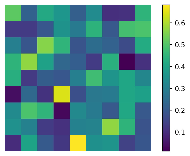
Figure 1: Action of $\mathcal{M}_{R}$ map, 1000 times, on a random seed unitary of size $d^{2}=9$ results in an approximate dual unitary which have typically all $d^{4}$ entries non-zero. Shown are the absolute value of the matrix elements in one such instance.

In this section we demonstrate that modified algorithms can be defined that are capable of resulting in dual and 2-unitaries with block-diagonal structures or enphased permutations, and hence afford some degree of control or design. This is achieved by incorporating in the algorithm random diagonal unitaries which preserve the dual-unitary property of structured matrices.

One such algorithm $\mathbb{M}_{R}$ which converges to dual unitaries with the enphasing symmetry is defined as

$$\mathbb{M}_{R}:\;\;U_{0}\xrightarrow{R}U_{0}^{R}\xrightarrow{\text{PD}}U_{1}^{\prime}\rightarrow U_{1}=D_{1}\;U_{1}^{\prime}\;D_{2}\;,$$ (25)

where $D_{1},\,D_{2}$ are diagonal unitaries with random phases. Note that the map is no longer deterministic, as $U_{0}$ does not uniquely determine $U_{1}$. The map converges (in all cases that we have encountered for $d=2,\,3,\,4$) to dual unitaries that remain dual-unitary on multiplication by arbitrary diagonal unitaries.

Starting from a random seed unitary $U_{0}$, the map converges to dual unitaries with different block structures as shown in Fig. (2) for $d^{2}=9$. For the sake of convenience we have shown the non-zero elements of the corresponding T-dual unitary to the dual-unitary obtained from the map. It is known that a block-diagonal unitary of size $d^{2}$ is T-dual if the size of each block is a multiple of $d$ Aravinda et al. (2021). The map indeed yields T-dual unitaries which are block-diagonal and size of each block is multiple of $d$ as shown in Fig. (2) for $d^{2}=9$. The resulting dual unitaries are of the following form (up to multiplication by $S$):

1. $U=\oplus_{i=1}^{3}u_{i},\;u_{i}\in\mathcal{U}(3).$

2. $U=u_{1}\oplus u_{2},\;u_{1}\in\mathcal{U}(6),\,u_{2}\in\mathcal{U}(3).$

Due to their peculiar structure these dual unitaries remain dual-unitary under multiplication by random diagonal unitaries. This is easy to see for the uniform block case as compared to the non-uniform case in Fig. (2). In the nonuniform case, the $6\times 6$ block cannot be replaced by an arbitrary unitary matrix. In fact $6\times 6$ unitary matrix acting on $\mathcal{C}^{2}\otimes\mathcal{C}^{3}$ should satisfy T-dual unitarity Aravinda et al. (2021). If we require in addition that the duality (or T-duality equivalently) is preserved under multiplication by diagonal unitaries, a subset is picked, an example being shown in Fig. (2). Note the peculiar structure of the $6\times 6$ block in the non-uniform case. It consists of three $2\times 2$ unitary matrices arranged in such a way that multiplication by arbitrary diagonal unitaries preserves T-duality.

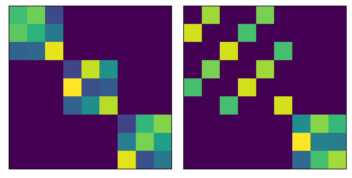
Figure 2: (Color online) Structured T-dual unitaries obtained using the $\mathbb{M}_{R}$ map for $d=3$. (Left) T-dual unitary consisting of three blocks (unitary matrices) of size 3. (Right) T-dual unitary with a $6\times 6$ block and a $3\times 3$ block.

We have checked that similar structured matrices are obtained for $d=4$ and $5$. For $d^{2}=16$, the map yields dual unitaries which are of the following forms (up to multiplication by $S$),

1. $U=\oplus_{i=1}^{4}u_{i}$, $u_{i}\in\mathcal{U}(4)$,

2. $U=\oplus_{i=1}^{2}u_{i}$, $u_{i}\in\mathcal{U}(8)$, and

3. $U=\oplus_{i=1}^{2}u_{i}$, $u_{1}\in\mathcal{U}(4)$, $u_{2}\in\mathcal{U}(12)$.

These block structures are compatible with the analytical constructions of dual unitary operators based on block-diagonal unitaries.

To obtain structured 2-unitaries, we define $\mathbb{M}_{\Gamma R}$ map as follows,

$$U_{0}\xrightarrow{R}U_{0}^{R}\xrightarrow{\Gamma}\left(U_{0}^{R}\right)^{\Gamma}:=U_{0}^{\Gamma R}\xrightarrow{\text{PD}}U_{1}^{\prime}\rightarrow U_{1}=D_{1}\;U_{1}^{\prime}\;D_{2}\;.$$ (26)

For $d^{2}=9$, it is observed that for a random seed unitary if the map converges to 2-unitary then it is a 2-unitary permutation matrix up to multiplication by diagonal unitaries as shown in Fig. (3). There is only one non-zero element in each row positioned in such a way that the whole arrangement of non-zero entries in a 2-unitary permutation matrix is directly related to orthogonal Latin squares which we elaborate in next sections. The map is not as efficient as it’s deterministric counterpart $\mathcal{M}_{\Gamma R}$ in yielding 2-unitaries from random seed unitaries. However, it demonstrates that one can obtain structured 2-unitary operators of desired symmetry and can be used to gain insights about the most general constructions of such special unitary operators,

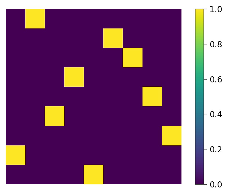
Figure 3: Action of $\mathbb{M}_{\Gamma R}$ map on a random seed unitary of order 9. The map converges to 2-unitary permutation matrix (up to phases). The only non-zero element in each row or column is shown by a yellow square.

We have observed that multiplying at each step of the map with random, but structured, unitaries other than diagonal unitaries can also yield structured dual matrices, provided duality is preserved under such operations.

IV Dynamical map in the two-qubit case

The $\mathcal{M}_{R}$ map is now studied explicitly and analytically in the case of two qubit unitary operators. The nonlocal part of the operators is well-known in this case. As the map has been shown to be covariant under local unitary transformations, see Eq. (18), it is sufficient to consider its action on the nonlocal part. The subset of dual-unitary matrices is known explicitly in this case and we can calculate the rate at which arbitrary seeds approach the dual set. We will find that those that approach the swap gate $S$ do so algebraically slowly, while generically the approach is exponential.

Any unitary operator in $\mathcal{U}(4)$ can be written as $(u_{1}\otimes u_{2})U(v_{1}\otimes v_{2})$, where $u_{i}$ and $v_{i}$ are single qubit unitaries in $\mathcal{U}(2)$, and

$$U=\exp\left[-i\sum_{k=1}^{3}c_{k}\,(\sigma_{k}\otimes\sigma_{k})\right].$$ (27)

Here $\sigma_{k}$ are Pauli matrices, $c_{k}\in\mathbb{R}$ are Cartan coefficients, and $U$ is the nonlocal part of the canonical Cartan form Khaneja et al. (2001); Kraus and Cirac (2001); Zhang et al. (2003). The so-called “Weyl chamber” Zhang et al. (2003) is a tetrahedron formed by considering the subset of $c_{k}$’s,

$$0\leq|c_{3}|\leq c_{2}\leq c_{1}\leq\frac{\pi}{4}$$ (28)

The $c_{k}$’s in the Weyl chamber which uniquely identify local unitarily inequivalent gates, is also termed as the gate’s information content Musz et al. (2013). The nonlocal part of $U$ we refer below simply as the Cartan form. For two qubit dual unitaries Bertini et al. (2019a),

$$c_{1}=c_{2}=\frac{\pi}{4},\;\;c_{3}\in\left[0,\frac{\pi}{4}\right],$$ (29)

and provides the complete parametrization of the nonlocal part. An equivalent parametrization is not known in higher dimensions.

IV.1 $\mathcal{M}_{R}$ map in the Weyl chamber

While the map has been defined on general unitary matrices, the overall phase has no impact on entanglement and the map can be defined as an action on $\mathcal{SU}(4)$, with $\det(U)=1$, to itself by removing the phase at each step. This turns out to be very useful for the qubit case.

Consider a seed unitary in Cartan form as

$$U_{0}=\exp\left[-i\sum_{k=1}^{3}c_{k}^{(0)}\,(\sigma_{k}\otimes\sigma_{k})\right]=$$ (30)

$$\left(\begin{array}[]{cccc}e^{-ic_{3}^{(0)}}c_{-}^{(0)}&0&0&-ie^{-ic_{3}^{(0)}}s_{-}^{(0)}\\ 0&e^{ic_{3}^{(0)}}c_{+}^{(0)}&-ie^{ic_{3}^{(0)}}s_{+}^{(0)}&0\\ 0&-ie^{ic_{3}^{(0)}}s_{+}^{(0)}&e^{ic_{3}^{(0)}}c_{+}^{(0)}&0\\ -ie^{-ic_{3}^{(0)}}s_{-}^{(0)}&0&0&e^{-ic_{3}^{(0)}}c_{-}^{(0)}\end{array}\right)$$

where,

$$\begin{split}c_{\pm}^{(n)}&=\cos(c_{1}^{(n)}\pm c_{2}^{(n)}),\\ s_{\pm}^{(n)}&=\sin(c_{1}^{(n)}\pm c_{2}^{(n)}),\;n=0,1,\cdots.\end{split}$$ (34)

Note that $U_{0}\in\mathcal{SU}(4)$ and we would like the subsequent iterations to also satisfy this property: it also becomes easy to identify the Cartan coefficients $c_{i}$ at every step. A crucial property of the map is that it preserves the matrix form of $U_{0}$ such that $U_{1}$ has exactly the same structure; see appendix (A).

Let

$$U_{n}=\left(\begin{array}[]{cccc}\alpha_{n}&0&0&\beta_{n}\\ 0&\delta_{n}&\gamma_{n}&0\\ 0&\gamma_{n}&\delta_{n}&0\\ \beta_{n}&0&0&\alpha_{n}\end{array}\right)\;\in\;\mathcal{SU}(4)\,,$$ (35)

where

$$\begin{split}&\alpha_{n}=e^{-ic_{3}^{(n)}}c_{-}^{(n)},\,\beta_{n}=-ie^{-ic_{3}^{(n)}}s_{-}^{(n)},\\ &\gamma_{n}=-ie^{ic_{3}^{(n)}}s_{+}^{(n)},\,\delta_{n}=e^{ic_{3}^{(n)}}c_{+}^{(n)},\end{split}$$ (36)

The mapping between matrix elements of $U_{n+1}$ and $U_{n}$ is given by

$$\begin{split}\alpha_{n+1}=&\frac{e^{-i\,\frac{\chi_{n+1}}{4}}}{2}\left[\frac{\alpha_{n}+\delta_{n}}{|\alpha_{n}+\delta_{n}|}+\frac{\alpha_{n}-\delta_{n}}{|\alpha_{n}-\delta_{n}|}\right]\\ \beta_{n+1}=&\frac{e^{-i\,\frac{\chi_{n+1}}{4}}}{2}\left[\frac{\alpha_{n}+\delta_{n}}{|\alpha_{n}+\delta_{n}|}-\frac{\alpha_{n}-\delta_{n}}{|\alpha_{n}-\delta_{n}|}\right]\\ \gamma_{n+1}=&\frac{e^{-i\,\frac{\chi_{n+1}}{4}}}{2}\left[\frac{\beta_{n}+\gamma_{n}}{|\beta_{n}+\gamma_{n}|}-\frac{\beta_{n}-\gamma_{n}}{|\beta_{n}-\gamma_{n}|}\right]\\ \delta_{n+1}=&\frac{e^{-i\,\frac{\chi_{n+1}}{4}}}{2}\left[\frac{\beta_{n}+\gamma_{n}}{|\beta_{n}+\gamma_{n}|}+\frac{\beta_{n}-\gamma_{n}}{|\beta_{n}-\gamma_{n}|}\right],\end{split}$$ (37)

where

$$\chi_{n+1}=\text{Arg}[(\alpha_{n}^{2}-\delta_{n}^{2})(\beta_{n}^{2}-\gamma_{n}^{2})].$$ (38)

The dynamical system is thus a 4-dimensional complex map on the manifold $S^{4}\times S^{4}$. There are constraints originating from the unitarity condition: $|\alpha_{i}|^{2}+|\beta_{i}|^{2}=1$, $|\gamma_{i}|^{2}+|\delta_{i}|^{2}=1$, $\mbox{Re}(\alpha_{i}\beta_{i}^{*})=0$ and $\mbox{Re}(\gamma_{i}\delta_{i}^{*})=0$, and the $\mathcal{SU}$ condition: $(\alpha_{n}^{2}-\beta_{n}^{2})(\delta_{n}^{2}-\gamma_{n}^{2})=1$. The nonlinear nature of the map is clear as the entries of the above transformation are themselves functions of other variables.

Rather than the high-dimensional complex map in Eq. (37), using Eq. (36) one obtains a 3-dimensional real map in terms of the Cartan coefficients. Defining $\theta_{\pm}^{(n)}=\text{Arg}(\alpha_{n}\pm\delta_{n})$ and $\phi_{\pm}^{(n)}=\text{Arg}(\beta_{n}\pm\gamma_{n})$, the complex map in Eq. (37) simplifies to

$$\begin{split}&c_{1}^{(n+1)}=\frac{1}{4}(-\theta_{+}^{(n)}+\theta_{-}^{(n)}-\phi_{+}^{(n)}+\phi_{-}^{(n)}),\\ &c_{2}^{(n+1)}=\frac{1}{4}(\theta_{+}^{(n)}-\theta_{-}^{(n)}-\phi_{+}^{(n)}+\phi_{-}^{(n)}),\\ &c_{3}^{(n+1)}=\frac{1}{4}(-\theta_{+}^{(n)}-\theta_{-}^{(n)}+\phi_{+}^{(n)}+\phi_{-}^{(n)}).\end{split}$$ (39)

Numerically it is observed that the Cartan coefficients of $U_{n+1}=\mathcal{M}_{R}[U_{n}]$ obtained from the above 3-dimensional map agree for all even $n$ with those calculated using the numerical algorithm presented in Refs. Childs et al. (2003); Musz et al. (2013) and also satisfy Eq. (28). However for odd $n$ although $c_{3}^{(n)}$ values still agree but $c_{1}^{(n+1)}$ and $c_{2}^{(n+1)}$ values differ from the numerical value by $\pi/2$. In order to obtain the desired Cartan coefficients satisfying Eq. (28) from the above 3-dimensional map, one needs to replace $c_{2}^{(n+1)}$ by $\pi/2-c_{2}^{(n+1)}$ for all odd $n$.

Before we simplify the 3-dimensional map given by Eq. (39), we first prove the following two theorems.

Theorem 1.

For two-qubit gates of the form Eq. (27) self-dual unitaries ($U=U^{R}$) are the only fixed points of the $\mathcal{M}_{R}$ map.

Theorem 2.

For two-qubit gates of the form Eq. (27) dual unitaries are the only fixed points of the $\mathcal{M}_{R}^{2}$ map i.e., $\mathcal{M}_{R}^{2}[U_{0}]=U_{0}$ iff $U_{0}$ is a dual-unitary.

Proofs of the above theorems are presented in appendix B.

Consider a two-qubit seed unitary $U_{0}$ parametrized by the Cartan parameters $c_{1}^{(0)},c_{2}^{(0)},c_{3}^{(0)}$. Under the $\mathcal{M}_{R}$ map $U_{0}$ is mapped to $U_{1}$ which is parametrized by $c_{1}^{(1)},c_{2}^{(1)},c_{3}^{(1)}$. The $\mathcal{M}_{R}$ map can be viewed most economically as a 3-dimensional dynamical map on the Cartan parameters,

$$\begin{split}U_{n}&\xrightarrow{\mathcal{M}_{R}}U_{n+1},\\ (c_{1}^{(n)},c_{2}^{(n)},c_{3}^{(n)})&\xrightarrow{\mathcal{M}_{R}}(c_{1}^{(n+1)},c_{2}^{(n+1)},c_{3}^{(n+1)}).\end{split}$$ (40)

IV.2 Deriving the map for special initial conditions

Although we are unable to derive explicit maps in terms of these parameters for general $c_{i}^{(0)}$, we are able to do so for special values. We show that these converge to the desired fixed points, $c_{1}^{(n\rightarrow\infty)}=\pi/4,\;c_{2}^{(n\rightarrow\infty)}=\pi/4\,,$ and $c_{3}^{(n\rightarrow\infty)}\in[0,\pi/4]$, which is the set of dual-unitary operators. This is depicted in Fig. (4) for few random realizations evolved under the map for $n=10$ steps.

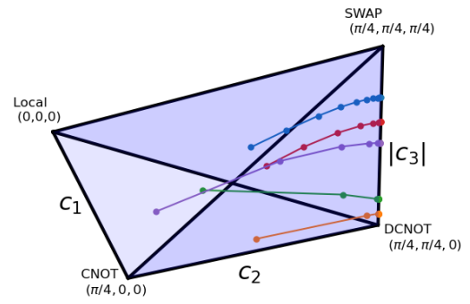
Figure 4: Trajectories of five random realizations of two-qubit gates are shown inside the Weyl chamber under action of the map for $n=10$ steps. The edge joining the swap gate and the dcnot gate corresponds to dual unitaries to which the map converges.

For the general case we argue why this happens and also derive the rate of exponential approach.

IV.2.1 XY family: plane $c_{3}=0$

The first special case is when $c_{3}^{(0)}=0$ and $0<c_{2}^{(0)}\leq c_{1}^{(0)}$. In this case, using Eq. (37), we can see that a single application of the $\mathcal{M}_{R}$ map results in the following unitary:

$$U_{1}=\left(\begin{array}[]{cccc}1&0&0&0\\ 0&0&-i&0\\ 0&-i&0&0\\ 0&0&0&1\end{array}\right),$$

with $\det(U_{1})=\det(U_{0})=1$. Thus the map preserves the $\mathcal{SU}$ property of seed unitaries. Cartan parameters for $U_{1}$ are: $c_{1}^{(1)}=c_{2}^{(1)}=\pi/4,\,c_{3}^{(1)}=0$, and therefore $U_{1}$ is dual-unitary. This gate is LU equivalent to the gate dcnot Musz et al. (2013) which is $S\times\mbox{{\sc cnot}}$. Explicitly,

$$U_{\text{DCNOT}} =(H\otimes I)\,U_{1}\,(D_{1}\otimes D_{1}\,H)$$

$$=\begin{pmatrix}1&0&0&0\\ 0&0&0&1\\ 0&1&0&0\\ 0&0&1&0\end{pmatrix},$$ (41)

where $H=\frac{1}{\sqrt{2}}\begin{pmatrix}1&1\\ 1&-1\end{pmatrix}$ is the Hadamard gate and $D_{1}=P_{\frac{\pi}{2}}=\begin{pmatrix}1&0\\ 0&i\end{pmatrix}$ is a phase gate.

Thus the entire interior of the base of the Weyl chamber, $c_{3}=0$ plane, is mapped to the same dual-unitary gate $U_{1}$ in just one step and the rate at which it happens is infinite.

IV.2.2 XXX family: $c_{1}=c_{2}=c_{3}$

Let $c_{1}=c_{2}=c_{3}=c\in[0,\pi/4]$ in Eq. (27), the single parameter family of unitary operators $U$,

$$U=\exp(-i\,c\sum_{i=1}^{3}\sigma_{i}\otimes\sigma_{i}).$$ (42)

This forms an edge of the Weyl chamber, the one that connects local unitaries to the swap gate $S$. Unitaries of this form are useful in many contexts such as in the trotterization of integrable isotropic (XXX) Heisenberg Hamiltonian Vanicat et al. (2018). They are also, modulo phases, the fractional powers of the swap gate $S$ as $U=\exp\left(-2\,i\,c\,S\right)$.

If we choose the seed unitary $U_{0}$ from this family with $c=c^{(0)}$, it follows from Eq. (36) that $\beta_{0}=0$. Action of the map on $U_{0}$ gives

$$U_{1}=\begin{pmatrix}\alpha_{1}&0&0&\beta_{1}\\ 0&0&\gamma_{1}&0\\ 0&\gamma_{1}&0&0\\ \beta_{1}&0&0&\alpha_{1}\end{pmatrix},$$ (43)

for which $\delta_{1}=0$. Note that $U_{1}$ is not exactly of the same form as $U_{0}$ for which $\beta_{0}=0$. In fact for all even (odd) $n$, $U_{n}$ is such that $\beta_{n}=0$ ($\delta_{n}=0$). For even $n$, $\beta_{n}=0$ implies $c_{1}{(n)}=c_{2}{(n)}$ both being equal to $c_{3}^{(n)}$ and thus $U_{n}$ belongs to the same family. However, for odd $n$ it is observed that although $c_{2}^{(n)}=c_{3}^{(n)}\leq\pi/4$, $c_{1}^{(1)}=\pi/2-c_{2}^{(1)}\geq\pi/4$ and thus $c_{1}^{(1)}$ does not satisfy Eq. (28). Note that $U_{1}$ with Cartan coefficients $c_{1}^{(1)}=\pi/2-c^{(1)},c_{2}^{(n)}=c_{3}^{(1)}=c^{(1)}$ is not LU equivalent to a gate with Cartan coefficients $c_{1}^{(n)}=c_{2}^{(n)}=c_{3}^{(1)}=c^{(1)}$, although in the part of the Weyl chamber we are restricted attention to, they are the same points.

As a consequence of this, the 3-dimensional map given by Eq. (39) becomes a 1-dimensional map.

Let $c^{(n)}$ be the Cartan coefficient parametrizing $U_{n}=\mathcal{M}_{R}^{n}[U_{0}]$, and

$$x_{n}=1/\tan(2\,c^{(n)}).$$ (44)

The complications attendant on the ranges of $c_{i}$ do not affect this variable. In terms of $x_{n}$ (for a derivation see App. (C)), the map takes a simple algebraic form,

$$x_{n+1}=\frac{2\,x_{n}}{1+\sqrt{4\,x_{n}^{2}+1}}.$$ (45)

The unique fixed point of the map is $x^{*}=0$ corresponding to the swap gate, and the map is a contraction as shown in the App. (C). Therefore, in the limit of large $n$, $x_{n}\rightarrow x^{*}=0$. In this limit, Eq. (45) can be approximated as

$$x_{n+1}\approx x_{n}(1-x_{n}^{2}).$$ (46)

Thus in the vicinity of the fixed point, the difference equation may be approximated by the differential equation $dx_{n}/dn=-x_{n}^{3}$. This is simple to solve and gives the large $n$ approximation to the map above as

$$x_{n}\approx 1/\sqrt{2n}.$$ (47)

IV.2.3 swap-cnot-dcnot face; $c_{1}^{(0)}=\pi/4$

In this case seed unitaries lie on the swap-cnot-dcnot face of the Weyl chamber with $c_{1}^{(0)}=\pi/4$. Under the action of the map $c_{1}^{(n)}=\pi/4$ for all $n$ and thus the corresponding map is 2-dimesional defined in terms of $c_{2}^{(n)}$ and $c_{3}^{(n)}$. An important property of the map observed in this case, which follows as $c_{\pm}=s_{\mp}$, is that the phase in Eq. (37) $\chi_{n+1}=0$. This property is crucial for simplifying the map as shown below.

Defining $y_{n}=1/\tan^{2}(2\,c_{2}^{(n)})$ and $z_{n}=1/\tan^{2}(2\,c_{3}^{(n)})$, the corresponding 2-dimensional map takes a purely algebraic form given by (for a derivation see App. (C))

$$\begin{split}y_{n+1}&=\frac{y_{n}}{1+z_{n}},\\ z_{n+1}&=\frac{z_{n}}{1+y_{n}}.\end{split}$$ (48)

Although the above map has a symmetric form, due to the specific choice of Cartan parameters Eq. (28), the symmetry is broken and the fixed points are $y^{*}=0$ (or $c_{2}^{(\infty)}=\pi/4$) and $z^{*}\in[0,\infty]$ (or $c_{3}^{(\infty)}\in[0,\pi/4]$) corresponding to the set of dual unitaries. This 2-dimensional map can be solved analytically by noting that

$$\Omega=\frac{1+y_{n+1}}{1+z_{n+1}}=\frac{1+y_{n}}{1+z_{n}}$$ (49)

is an invariant. It’s value is determined by the initial conditions as:

$$\Omega=\frac{1+y_{0}}{1+x_{0}}=\left(\frac{\sin(2\,c_{3}^{(0)})}{\sin(2\,c_{2}^{(0)})}\right)^{2}<1$$ (50)

for $c_{3}^{(0)}<c_{2}^{(0)}$.

Using this to eliminate $z_{n}$, we have the 1-dimensional map:

$$\begin{split}y_{n+1}=\Omega\frac{y_{n}}{1+y_{n}},\end{split}$$ (51)

which has the exact solution

$$y_{n}=\frac{\Omega^{n}\,y_{0}}{1+\left(\dfrac{1-\Omega^{n}}{1-\Omega}\right)\,y_{0}},$$ (52)

and implies that

$$z_{n}=\frac{z_{0}}{\Omega^{n}+\left(\dfrac{1-\Omega^{n}}{1-\Omega}\right)\,\Omega\,z_{0}}.$$ (53)

It follows from Eq. (52) that $y_{\infty}=0$ and $z_{\infty}=\frac{1}{\Omega}-1$ respectively. Also $c_{3}^{(\infty)}$ which parametrizes the dual unitary to which the map converges can be written explicity in terms of the initial pair $(c_{2}^{(0)},c_{3}^{(0)})$ as

$$\begin{split}c_{3}^{(\infty)}&=\frac{1}{2}\arctan\left[\sqrt{\frac{\Omega}{1-\Omega}}\right]\\ &=\frac{1}{2}\arctan\left[\frac{\sin(2\,c_{3}^{(0)})}{\sqrt{\sin^{2}(2\,c_{2}^{(0)})-\sin^{2}(2\,c_{3}^{(0)})}}\right].\end{split}$$ (54)

Defining $\Delta c_{i}^{(n)}=c_{i}^{(\infty)}-c_{i}^{(n)}$ where $c_{1}^{(\infty)}=c_{2}^{(\infty)}=\pi/4$. Note that $\Omega=\sin^{2}(2\,c_{3}^{(\infty)})$, governs the exponential approach to the duals. From the explicit and full solution in Eq. (52) it follows that

$$\begin{split}\Delta c_{2}^{(n)}&\sim|\sin 2\,c_{3}^{(\infty)}|^{n},\\ \Delta c_{3}^{(n)}&\sim|\sin 2\,c_{3}^{(\infty)}|^{2\,n}.\end{split}$$ (55)

We will see below that these continue to hold for the general case as well.

The marginal case $\Omega=1$ corresponds to seed unitaries on the swap-cnot edge with $c_{2}^{(0)}=c_{3}^{(0)}$ and is dealt separately below.

IV.2.4 swap-cnot edge

For these gates $c_{1}^{(0)}=\pi/4,\,c_{2}^{(0)}=c_{3}^{(0)}$ and is a special case of the face just discussed. In this case, the 2-dimensional map Eq. (48) degenerates to a 1-dimensional map given by

$$y_{n+1}=\frac{y_{n}}{1+y_{n}},$$ (56)

with $\Omega=1$. This map also can be solved analytically and the solution is given by

$$y_{n}=\frac{y_{0}}{\sqrt{n\,y_{0}^{2}+1}}.$$ (57)

The approach to the unique fixed point $y^{*}=0$ is algebraic in contrast to other gates on the swap-cnot-dcnot face and goes as $\sim 1/\sqrt{n}$. Thus the swap gate is approached slowly along both the edges that connect it in the Weyl chamber from the locals or from the cnot gates. The other edge is the dual-unitary edge that is already a line of fixed points. In fact the entire face of the Weyl chamber containing locals-swap-cnot is mapped into itself and all initial conditions on this approach the dual-unitary swap gate algebraically. This face is characterized by two of the Cartan coefficients being equal, namely $c_{2}^{(n)}=c_{3}^{(n)}\equiv c^{(n)}$. In the limit of large $n$, $\Delta c_{1}^{(n)}=\pi/4-c_{1}^{(n)}\sim 1/n$ while $\Delta c_{2}^{(n)}=\Delta c_{3}^{(n)}=\pi/4-c^{(n)}\sim 1/\sqrt{n}$.

IV.2.5 XXZ family: $c_{1}=c_{2}$

Let us consider now a family of two-qubit gates for which $c_{1}^{(0)}=c_{2}^{(0)}=c^{(0)}\in(0,\frac{\pi}{4}]$, and $c_{3}^{(0)}\leq c^{(0)}\in[0,\frac{\pi}{4}]$. This restricts the seed unitaries to the face of the Weyl chamber that contains locals-swap-dcnot. Under the action of the map the unitaries remain on this face for even $n$ and up to a local unitary transformation for odd $n$.

The map is 2-dimensional defined on $c_{1}^{(n)}=c_{2}^{(n)}=c^{(n)}\leq\pi/4$ and $c_{3}^{(n)}\leq c^{(n)}$ is given by

$$c^{(n+1)} =\frac{\pi}{4}-\frac{1}{4}\arctan\left\{\frac{1}{2}\sin(2\,c_{3}^{(n)})\left[\frac{1}{\tan^{2}(c^{(n)})}-\tan^{2}(c^{(n)})\right]\right\},$$ (58)

$$c_{3}^{(n+1)} =\frac{c_{3}^{(n)}}{2}+\frac{1}{4}\arctan\left\{\frac{1}{2}\tan(2\,c_{3}^{(n)})\left[\frac{1}{\tan^{2}(c^{(n)})}+\tan^{2}(c^{(n)})\right]\right\},$$ (59)

The fixed points consist of $c^{*}=\pi/4$ and $c_{3}^{*}$ can take any value in $[0,\frac{\pi}{4}]$ which is a line of fixed points corresponding to two-qubit dual unitaries. It is not hard to see that these are the only fixed points of the map.

The important information about the nature of the map can be obtained in the large $n$ limit, which is effectively a linear stability analysis. Defining $\Delta c_{i}^{(n)}=c_{i}^{(\infty)}-c_{i}^{(n)}$ where $c_{1}^{(\infty)}=c_{2}^{(\infty)}=\pi/4$. For small $\Delta c^{(n)}$, Eq. (58) gives

$$\Delta c^{(n+1)}\approx\sin(2\,c_{3}^{(n)})\Delta c^{(n)}.$$ (60)

Whereas Eq. (59) yields simply $c_{3}^{(n+1)}\approx c_{3}^{(n)}$ to first order in $X_{n}$ indicating that it can take any value only determined by the initial condition. We denote this value as $c_{3}^{*}=c_{3}^{(\infty)}$. Thus the above equation is of the form, $\Delta c^{(n+1)}=r\Delta c^{(n)}$, with $r=\sin(2\,c_{3}^{(\infty)})$ , and we get the solution:

$$\Delta c^{(n)}=e^{-n\xi}\Delta c^{(0)},\;\xi=|\ln r|=\left|\ln\sin(2\,c_{3}^{(\infty)})\right|$$ (61)

Therefore, the convergence to the respective fixed points: $c^{*}=\frac{\pi}{4}$ and $c_{3}^{*}=c_{3}^{(\infty)}\in[0,\pi/4]$, is also exponential with the rate determined by the value $c_{3}^{(\infty)}$ as found in Eq. (55) for gates lying on the swap-cnot-dcnot face. This is shown qualitatively in Fig. (5). The rate $\xi=\infty$ when $c_{3}^{(\infty)}=0$ and the unitaries converge to the dcnot. This is consistent with the discussion in the XY discussion above where it was shown that in this case just one step of the map is needed. The rate $\xi=0$ when $c_{3}^{(\infty)}=\pi/4$ when the gate attained aymptotically is the swap. This is consistent with the discussion of the edge XXX above where an algebraic approach was obtained.

For large $n$ the behaviour of $\Delta c_{3}^{(n+1)}=c_{3}^{(\infty)}-c_{3}^{(n)}$ is found by analyzing Eq. (59) keeping the second order terms in $\Delta c^{(n)}$, and we get

$$\Delta c_{3}^{(n+1)}=\frac{1}{2}\sin(4c_{3}^{(\infty)})(\Delta c^{(n)})^{2}=\frac{1}{2}\sin(4c_{3}^{(\infty)})e^{-n\xi_{3}},$$ (62)

with $\xi_{3}=2\xi$, and hence the approach to $c_{3}^{(\infty)}$ is exponential at a rate that is twice that of the other Cartan parameters.

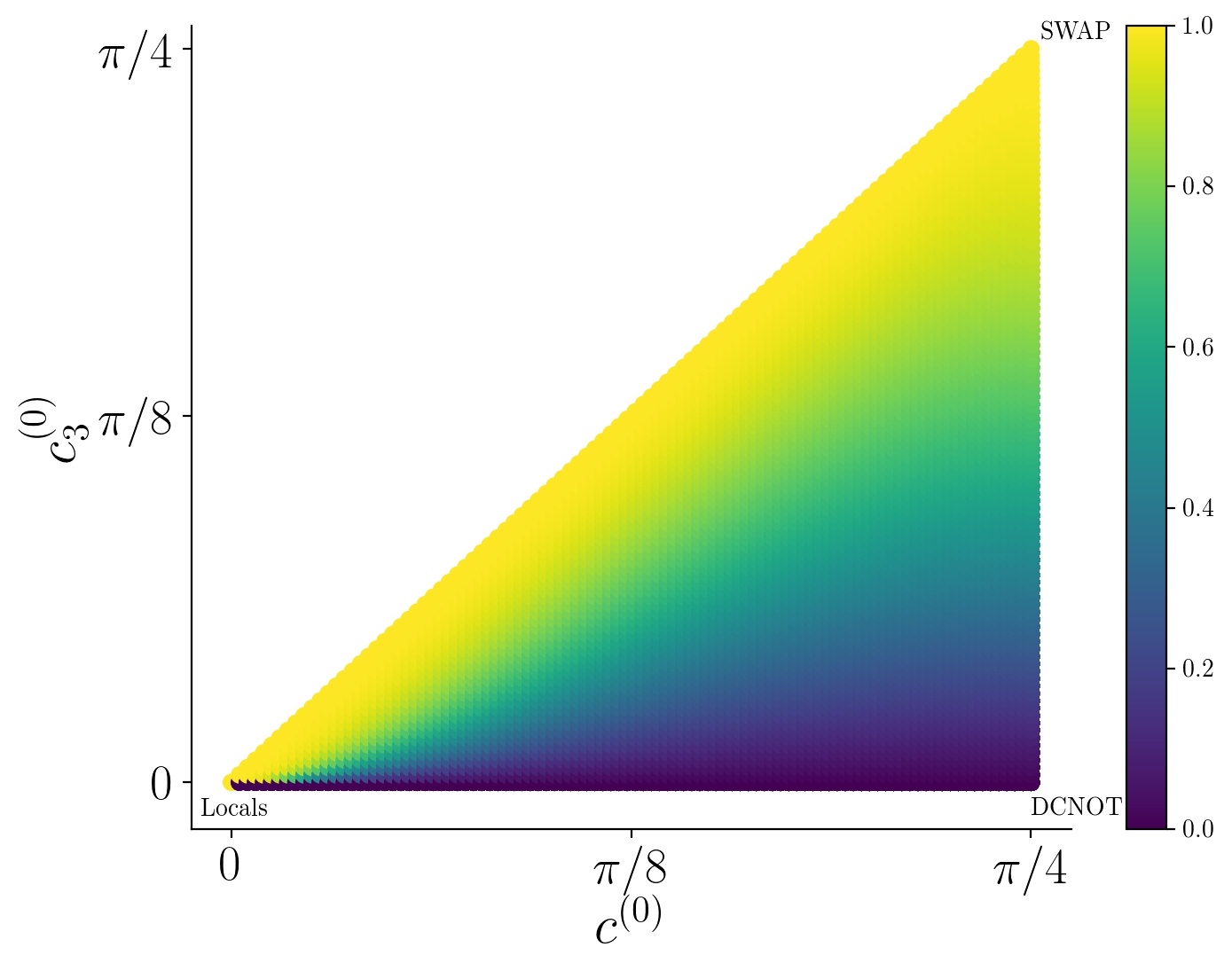
Figure 5: Convergence in the XXZ case: initial condition in the local-swap-dcnot face. Plotted is $r=\sin{(2\,c_{3}^{(100)})}\approx\sin{(2\,c_{3}^{(\infty)})}$, which is related to the rate of convergence to a dual-unitary gate as $\xi=\ln r$. Around $10^{5}$ initial conditions $(c^{(0)},c_{3}^{(0)})$ are taken and evolved for $n=100$ times under the 2-d map Eqs. ( 58)– (59). Initial conditions with $c_{3}^{(0)}=0$, in the base of the triangle above, converge to the dcnot gate at an infinite rate, while initial conditions with $c^{(0)}=c_{3}^{(0)}\in(0,\pi/4]$ converge to the swap gate at vanishing rate, namely algebraically.

IV.2.6 Generic initial conditions

Interestingly, numerical results indicate that the exponential approach to $(\pi/4,\pi/4,c_{3}^{(\infty)})$ given in Eq. (61) and Eq. (62) continues to hold for a generic initial condition inside the Weyl chamber. An illustration is displayed in Fig. (6) for the initial condition $(c_{1}^{(0)},c_{2}^{(0)},c_{3}^{(0)})=(\pi/6,\pi/8,\pi/12)$. Under the map it converges to a dual-unitary gate with $c_{3}^{\infty}\approx 0.443$. The rates $\xi_{1}$ and $\xi_{2}$ at which $\Delta c_{1}^{(n)}=\pi/4-c_{1}^{(n)}$ and $\Delta c_{2}^{(n)}=\pi/4-c_{2}^{(n)}$ approach $0$ are almost the same given by $\xi=\left|\ln\sin(2\,c_{3}^{(\infty)})\right|$. The rate $\xi_{3}$ at which $\Delta c_{3}^{(n)}=c_{3}^{(\infty)}-c_{3}^{(n)}\rightarrow 0$ continues to be a very good approximation $\xi_{3}=2\xi$. Initial conditions which converge to dual-unitaries with large $c_{3}^{(\infty)}$ values i.e., small entangling power, take longer times. This is reflected in Fig. (4) for random realizations where gates that are closer to the swap gate take longer to reach the corresponding point on the dual-unitary edge.

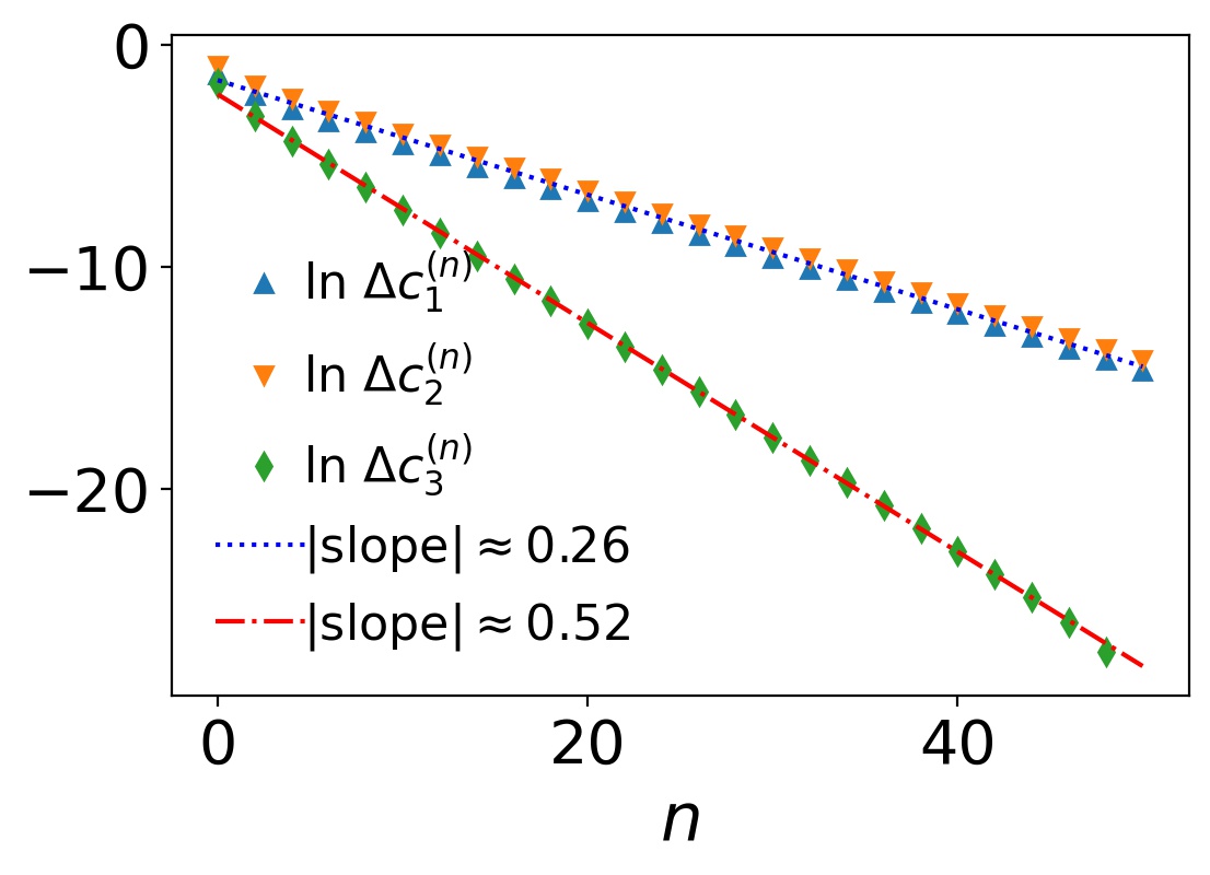
Figure 6: Convergence for initial condition inside the Weyl chamber: seed unitary with $(c_{1}^{(0)},c_{2}^{(0)},c_{3}^{(0)})=(\pi/6,\pi/8,\pi/12)$ is evolved under the map for $n=50$ steps. The exponential rates at which $\Delta c_{1}^{(n)}=\pi/4-c_{1}^{(n)}$ and $\Delta c_{2}^{(n)}=\pi/4-c_{2}^{(n)}$ decay are almost the same $\xi=|\ln\sin(2c_{3}^{(\infty)})|$ determined by $c_{3}^{(\infty)}\approx 0.443$. Rate at which $\Delta c_{3}^{(n)}=c_{3}^{(\infty)}-c_{3}^{(n)}\rightarrow 0$ is almost twice than that of $\Delta c_{1}^{(n)}$ or $\Delta c_{2}^{(n)}$. The numerically calculated slopes match with these values.

We summarize the convergence of the map for different families in Table 1. The slow algebraic approach hold for all initial conditions that approach the swap gate. In fact, we have numerically verified that even for higher dimensions, $d>2$, if the seed unitary is a fractional power of swap, they approach the dual-unitary swap gate algebraically as $\sim 1/\sqrt{n}$.

It maybe noted that a very different map on the Weyl chamber has been studied by looking at the the powers of two-qubit gates in Ref. Mandarino et al. (2018). This map is ergodic on the Weyl chamber and is related to billiard dynamics in a tetrahedron, unlike the dissipative nature of the $\mathcal{M}_{R}$ map that we have studied.

Table 1: Convergence to dual unitaries for different two-qubit seed unitaries, parametrized by the Cartan coefficients $c_{i}^{(0)}$. In all cases $c_{1}^{(\infty)}=c_{2}^{(\infty)}=\pi/4$, and $\Delta c_{i}=c_{i}^{(\infty)}-c_{i}^{(n)}$.

Cartan coefficients and Weyl chamber location of seeds	Dual-unitary approached	Nature of convergence
Base, $c_{3}^{(0)}=0$, $c_{2}^{(0)}>0$	dcnot, $c_{3}^{(1)}=\,c_{3}^{(\infty)}=0$	Instantaneous, rate $\infty$
swap-Local Edge: $c_{1}^{(0)}=c_{2}^{(0)}=c_{3}^{(0)}$	swap	Algebraic: $\Delta c_{i}\sim 1/\sqrt{n}$
swap-Local-cnot face, $c_{2}^{(0)}=c_{3}^{(0)}\neq c_{1}^{(0)}$	$c_{3}^{(\infty)}=\pi/4$	Algebraic: $\Delta c_{3},\,\Delta c_{2}\sim 1/\sqrt{n},\,\Delta c_{1}\sim 1/n$
swap-Local-dcnot face, $c_{1}^{(0)}=c_{2}^{(0)}\neq c_{3}^{(0)}$		Exponential:
swap-cnot-dcnot face, $c_{1}^{(0)}=\pi/4$, $c_{2}^{(0)}\neq c_{3}^{(0)}$	Generic	$\Delta c_{1},\Delta c_{2}\sim\exp(-\xi\,n),\,\Delta c_{3}\sim\exp(-2\xi\,n)$
Interior, $c_{1}^{(0)}>c_{2}^{(0)}>c_{3}^{(0)}$	$c_{3}^{(\infty)}\neq 0,\,\pi/4$	$\xi=|\ln\sin(2c_{3}^{(\infty)})|$

V Combinatorial designs corresponding to dual unitary operators

Tools developed in combinatorial mathematics have been very useful in constructing multipartite entangled states Goyeneche et al. (2015, 2018). In Ref. Clarisse et al. (2005) it was shown that orthogonal Latin squares of order $d$ can be used to contruct 2-unitary permutation matrices of order $d^{2}$. Since 2-unitary operators belong to a subset of dual-unitary operators, we point to less restrictive combinatorial structures corresponding to general dual-unitary operators. In the case of dual-unitary permutations such designs were discussed earlier in S et al. (2020), which we first summarize.

V.1 Permutation matrices: classical design

A permutation of $d^{2}$ symbols or elements from $\left[d\right]\times\left[d\right]$, $\left[d\right]=\left\{{1,2,\cdots,d}\right\}$, is specified by the operator on computational product basis states $\ket{ij}$ as,

$$P\ket{ij}=\ket{k_{ij}l_{ij}}.$$ (63)

Thus, this can be written in terms of a pair of $d\times d$ matrices $K=(k_{ij})$ and $L=(l_{ij})$. In Aravinda et al. (2021), it was shown that for $P$ to be dual-unitary (T-dual), the conditions on $K$ and $L$ matrices are:

1. Condition on $K$: No element repeats along any row (column).

2. Condition on $L$: No element repeats along any column (row).

As an example, for $d=2$, the dual-unitary swap gate permutes the basis states as

$$\begin{array}[]{|cc|}\hline\cr 11&12\\ 21&22\\ \hline\cr\end{array}\;\longrightarrow\;\begin{array}[]{|cc|}\hline\cr 11&21\\ 12&22\\ \hline\cr\end{array},$$ (64)

with $K$ and $L$ given by

$$K=\begin{array}[]{|cc|}\hline\cr 1&2\\ \hline\cr 1&2\\ \hline\cr\end{array}\;,\;L=\begin{array}[]{|c|c|}\hline\cr 1&1\\ 2&2\\ \hline\cr\end{array}.$$ (65)

Orthogonal Latin squares, denoted OLS$(d)$ Keedwell and Dénes (2015), are examples of designs used to construct the 2-unitary operators Clarisse et al. (2005). A Latin square is a $d\times d$ array with $d$ distinct elements such that every element appears exactly once in each column and in each row. Two Latin squares with elements $s_{ij}$ and $t_{ij}$ are orthogonal if the ordered pairs $(s_{ij},t_{ij})$ are all distinct.

If $K$ and $L$, defined above, are Latin squares, then the corresponding permutation matrix $P$ is both dual-unitary and T-dual, hence it is 2-unitary. OLS($d$) exist for all $d$ except $d=2$ and $6$ Bose et al. (1960). Thus 2-unitary permutations exist for all $d$ except $d=2$ and $6$. An example of an OLS($3$) is:

$$\begin{array}[]{|c|c|c|}\hline\cr 1&2&3\\ \hline\cr 3&1&2\\ \hline\cr 2&3&1\\ \hline\cr\end{array}\;\cup\;\begin{array}[]{|c|c|c|}\hline\cr 1&3&2\\ \hline\cr 3&2&1\\ \hline\cr 2&1&3\\ \hline\cr\end{array}\;=\;\begin{array}[]{|c|c|c|}\hline\cr 11&23&32\\ \hline\cr 33&12&21\\ \hline\cr 22&31&13\\ \hline\cr\end{array}.$$ (66)

Note that all nine pairs from the set $\left\{1,2,3\right\}\times\left\{1,2,3\right\}=\left\{11,12,\dots,32,33\right\}$ are present.

For dual-unitary or, T-dual permutations $K$ and $L$ are not Latin squares in general. We define r-Latin square (c-Latin square) as an arrangement of $d$ symbols in a $d\times d$ array if it satisfies conditions of a Latin square only along rows (columns). Note that the usual Latin square is both r-Latin square as well as c-Latin square. Two such less constrained Latin squares are orthogonal if by superposing them all $d^{2}$ ordered pairs obtained are distinct. For dual-unitary permutations $K$ is r-Latin square and $L$ is c-Latin square while for T-dual permutations $K$ is c-Latin square and $L$ is r-Latin square, which are restatements of the conditions above for duality (T-duality).

V.2 General dual-unitary operators: Quantum design

Here we discuss the underlying combinatorial structure of general dual-unitary operators. Consider a unitary operator $U\in\mathcal{B}(\mathcal{H}_{d}\otimes\mathcal{H}_{d})$. Define

$$\ket{\psi_{ij}}=U\ket{ij},$$ (67)

where $\{\ket{ij}\}_{i,j=1}^{d}$ is the computational basis in $\mathcal{H}_{d}\otimes\mathcal{H}_{d}$. The unitarity of $U$ implies that the set of vectors $\{\ket{\psi_{ij}}\}_{i,j=1}^{d}$ also forms an orthonormnal basis in $\mathcal{H}_{d}\otimes\mathcal{H}_{d}$.

Consider $\ket{\psi_{ij}}$’s which are of product form

$$\ket{\psi_{ij}}=\ket{\alpha_{ij}}\otimes\ket{\beta_{ij}}.$$ (68)

Analagous to $K$ and $L$ defined in the previous section for permutation operators, we arrange $d^{2}$ single qudit states $\ket{\alpha_{ij}}$ and $\ket{\beta_{ij}}$ as follows:

$$\begin{split}\mathcal{K}&=\begin{array}[]{|cccc|}\hline\cr\ket{\alpha_{11}}&\ket{\alpha_{12}}&\cdots&\ket{\alpha_{1d}}\\ \ket{\alpha_{21}}&\ket{\alpha_{22}}&\cdots&\ket{\alpha_{2d}}\\ \vdots&\vdots&\vdots&\vdots\\ \ket{\alpha_{d1}}&\ket{\alpha_{d2}}&\cdots&\ket{\alpha_{dd}}\\ \hline\cr\end{array}\\ \mathcal{L}&=\begin{array}[]{|cccc|}\hline\cr\ket{\beta_{11}}&\ket{\beta_{12}}&\cdots&\ket{\beta_{1d}}\\ \ket{\beta_{21}}&\ket{\beta_{22}}&\cdots&\ket{\beta_{2d}}\\ \vdots&\vdots&\vdots&\vdots\\ \ket{\beta_{d1}}&\ket{\beta_{d2}}&\cdots&\ket{\beta_{dd}}\\ \hline\cr\end{array}\end{split}$$ (69)

The conditions for $U$ to be dual-unitary in terms of $\mathcal{K}$ and $\mathcal{L}$ is presented below.

Theorem 3.

If every row of $\mathcal{K}$ and every column of $\mathcal{L}$ forms an orthonormal basis in $\mathcal{H}_{d}$, then the unitary operator $U=\sum_{i,j=1}^{d}\outerproduct{\psi_{ij}}{ij}=\sum_{i,j=1}^{d}\outerproduct{\alpha_{ij}\beta_{ij}}{ij}$ is dual-unitary.

Proof.

The orthonormality condition on the vectors in every row of $\mathcal{K}$ and every column of $\mathcal{L}$ imply that $\langle\alpha_{ij}|\alpha_{ij^{\prime}}\rangle=\delta_{jj^{\prime}},\;\sum_{j=1}^{d}\ket{\alpha_{ij}}\bra{\alpha_{ij}}=I_{d},\;\forall\>i$ and $\langle\beta_{ij}|\beta_{i^{\prime}j}\rangle=\delta_{ii^{\prime}},\;\sum_{i=1}^{d}\ket{\beta_{ij}}\bra{\beta_{ij}}=I_{d},\;\forall\>j$. Using these conditions, it follows,

$$U^{R}U^{R\dagger} =\left(\sum_{i,j=1}^{d}\ket{\alpha_{ij}i}\bra{\beta_{ij}j}\right)\left(\sum_{i^{\prime},j^{\prime}=1}^{d}\ket{\beta_{i^{\prime}j^{\prime}}j^{\prime}}\bra{\alpha_{i^{\prime}j^{\prime}}i^{\prime}}\right),$$

$$=\left(\sum_{j=1}^{d}\ket{\alpha_{ij}}\bra{\alpha_{ij}}\right)\otimes\left(\sum_{i=1}^{d}\ket{i}\bra{i}\right),$$

$$=I_{d}\otimes I_{d}=I_{d^{2}}.$$

It is similarly shown that $U^{R\dagger}U^{R}=I_{d^{2}}$, and hence unitary $U$ is dual-unitary. ∎

The conditions on $\mathcal{K}$, $\mathcal{L}$ for $U$ to be dual-unitary are generalizations of $K$ and $L$ corresponding to dual-unitary permutations. In $K$, $L$ the notion of symbols being different in row or column is replaced by it’s quantum analog, the orthogonality of vectors (quantum states). In fact such a generalization is known for Latin square and OLS called as quantum Latin square (QLS) Musto and Vicary (2016) and orthogonal quantum Latin square (OQLS) Goyeneche et al. (2018); Musto and Vicary (2019) respectively. A quantum Latin square is a $d\times d$ array of $d$-dimensional vectors such that each row and each column forms an orthonormal basis in $\mathcal{H}_{d}$. Two quantum Latin squares are orthogonal if together they form an orthonormal basis in $\mathcal{H}_{d}\otimes\mathcal{H}_{d}$. If $\mathcal{K}$, $\mathcal{L}$ defined above are quantum Latin squares then $U$ is a 2-unitary operator Goyeneche et al. (2018).

The fact that there are no repetitions of symbols in a Latin square in any row or column translates into orthogonality of vectors in each row and column in the corresponding QLS. The “quantumness” and equivalence between quantum Latin squares was defined in Ref. Paczos et al. (2021) in terms of the number of distinct basis vectors (up to phases), known as the cardinality. For QLS constructed from classical Latin squares, simply by replacing the symbol $k$ by a basis vector $\ket{k}$ in a $d$ dimensional space, the cardinality is $d$ and is said to be classical.

Quantum Latin square with cardinality more than $d$ cannot be obtained from classical Latin square using unitary transformations of the basis vectors and is referred to as genuinely quantum Paczos et al. (2021). Quantum Latin squares with cardinality equal to $d^{2}$, the maximum possible value, for general $d$ and their relation to quantum sudoku is discussed in Refs. Paczos et al. (2021); Nechita and Pillet .

For dual-unitary or, T-dual unitary operators $\mathcal{K}$ and $\mathcal{L}$ are not quantum Latin squares in general. We define r-quantum Latin square (c-quantum Latin square) denoted by r-QLS (c-QLS) as a $d\times d$ array of $d$-dimensional vectors if it satisfies conditions of a quantum Latin square only along rows (columns). Note that the quantum Latin square is both r-QLS as well as c-QLS. For dual-unitary operators $\mathcal{K}$ is r-QLS and $\mathcal{L}$ is c-QLS while for T-dual operators $\mathcal{K}$ is c-QLS and $\mathcal{L}$ is r-QLS.

Two such less constrained QLS are said to be orthogonal if together they form an orthonormal basis in $\mathcal{H}_{d}\otimes\mathcal{H}_{d}$. In analogy with cardinality of a quantum Latin square, we define cardinality of $\mathcal{K}$ or $\mathcal{L}$ as the number of distinct basis vectors (up to phases) they contain. An r-QLS or c-QLS of size $d$ is classical if it contains $d$ distinct basis vectors and genuinely quantum if it contains more than $d$ distinct basis vectors. For dual-unitary permutations cardinality of $\mathcal{K}$, $\mathcal{L}$ is always equal to $d$ and are thus classical. An example of a pair of genuine r-QLS and c-QLS of size $3$ are respectively,

$$\mathcal{K}:\begin{array}[]{|c c c|}\hline\cr\ket{1}&\ket{2}&\ket{3}\\ \hline\cr\ket{1}&\ket{2}&\ket{3}\\ \hline\cr\frac{1}{\sqrt{2}}\left(\ket{1}+\ket{2}\right)&\frac{1}{\sqrt{2}}\left(\ket{1}-\ket{2}\right)&\ket{3}\\ \hline\cr\end{array}\;,$$ (70)

$$\mathcal{L}:\begin{array}[]{|c|c|c|}\hline\cr\ket{1}&-\ket{1}&\frac{1}{\sqrt{2}}\left(\ket{1}+\ket{2}\right)\\ \ket{2}&\ket{2}&\ket{3}\\ \ket{3}&\ket{3}&\frac{1}{\sqrt{2}}\left(\ket{1}-\ket{2}\right)\\ \hline\cr\end{array}\;.$$ (71)

Note that both $\mathcal{K}$ (r-QLS) and $\mathcal{L}$ (c-QLS) contain five distinct basis vectors (quantum states), across two different orthonormal bases, and are thus genuinely quantum. Together $\mathcal{K}$ and $\mathcal{L}$ form an orthonormal basis in $\mathcal{H}_{3}\otimes\mathcal{H}_{3}$ arranged in $d\times d$ array as,

$$\small{\begin{array}[]{|c | c | c|}\hline\cr\ket{1}\otimes\ket{1}&-\ket{2}\otimes\ket{1}&\ket{3}\otimes\frac{1}{\sqrt{2}}\left(\ket{1}+\ket{2}\right)\\ \hline\cr\ket{1}\otimes\ket{2}&\ket{2}\otimes\ket{2}&\ket{3}\otimes\ket{3}\\ \hline\cr\frac{1}{\sqrt{2}}\left(\ket{1}+\ket{2}\right)\otimes\ket{3}&\frac{1}{\sqrt{2}}\left(\ket{1}-\ket{2}\right)\otimes\ket{3}&\ket{3}\otimes\frac{1}{\sqrt{2}}\left(\ket{1}-\ket{2}\right)\\ \hline\cr\end{array}\;}.$$ (72)

The dual-unitary gate corresponding to the above arrangement of size 9 is,

$$U_{9}=\left(\begin{array}[]{ccccccccc}1&0&0&0&0&0&0&0&0\\ 0&0&0&1&0&0&0&0&0\\ 0&0&0&0&0&0&\frac{1}{\sqrt{2}}&\frac{1}{\sqrt{2}}&0\\ 0&-1&0&0&0&0&0&0&0\\ 0&0&0&0&1&0&0&0&0\\ 0&0&0&0&0&0&\frac{1}{\sqrt{2}}&-\frac{1}{\sqrt{2}}&0\\ 0&0&\frac{1}{\sqrt{2}}&0&0&0&0&0&\frac{1}{\sqrt{2}}\\ 0&0&\frac{1}{\sqrt{2}}&0&0&0&0&0&-\frac{1}{\sqrt{2}}\\ 0&0&0&0&0&1&0&0&0\end{array}\right),$$ (73)

with $(e_{p}(U_{9}),g_{t}(U_{9}))=(3/4,5/8)$. This dual unitary is not locally equivalent to any dual unitary permutation matrix (corresponding $\mathcal{K}$ and $\mathcal{L}$ contain only three distinct vectors) with the same entangling power and gate-typicality. We obtained dual-unitary $U_{9}$ using the $\mathcal{M}_{R}$ map (see Sec. (III.1). This is one of the nice properties of the map that it yields structured dual-unitaries by choosing appropriate seed unitaries like permutations. For $e_{p}(U)<1$, it is relatively easier to construct dual unitaries which are LU inequivalent to dual unitary permutations with the same entangling power. However for $e_{p}(U)=1$ i.e., 2-unitaries this is not the case as they satisfy additional constraints which we discuss in the next section.

V.3 Combinatorial structures of known families of dual unitaries

V.3.1 Diagonal ensemble

Dual unitaries have one-to-one correspondence with T-dual unitary operators which are easier to construct. Simplest ensemble of T-dual unitaries one can think of is that of diagonal unitaries with arbitrary phases, denoted $D_{1}$. A $d^{2}$ parameter subset of dual unitaries can be obtained by (pre- or post-) multiplying diagonal unitaries with the swap gate $S$ Claeys and Lamacraft (2021); Aravinda et al. (2021). It is easy to see that for dual unitaries of the form $U=D_{1}S$ obtained from the diagonal ensemble,

$$U(\ket{k}\otimes\ket{l})=D_{1}S(\ket{k}\otimes\ket{l})=\exp(i\,\theta_{lk})(\ket{l}\otimes\ket{k}).$$ (74)

Thus, the corresponding $\mathcal{K}$ and $\mathcal{L}$ are same as that of the swap gate (up to phases) and hence are classical.

V.3.2 Block-diagonal ensemble

A more general $d^{3}$ parameter family of dual unitary gates, $U=D_{d}S$, can be obtained from block-diagonal unitaries Aravinda et al. (2021); Prosen (2021); Borsi and Pozsgay (2022), given by

$$D_{d}=\sum_{i=1}^{d}\ket{i}\bra{i}\otimes u_{i},\;u_{i}\in\mathcal{U}(d).$$ (75)

This is a controlled unitary from first subsystem to the second. For this family of dual unitaries the combinatorial structures are given by

$$\mathcal{K}:\begin{array}[]{|c c c c|}\hline\cr\ket{1}&\ket{2}&\cdots&\ket{d}\\ \hline\cr\ket{1}&\ket{2}&\cdots&\ket{d}\\ \hline\cr\vdots&\vdots&\vdots&\vdots\\ \hline\cr\ket{1}&\ket{2}&\cdots&\ket{d}\\ \hline\cr\end{array}\;\;,\;\mathcal{L}:\begin{array}[]{|c|c|c|c|}\hline\cr u_{1}\ket{1}&u_{2}\ket{1}&\cdots&u_{d}\ket{1}\\ u_{1}\ket{2}&u_{2}\ket{2}&\cdots&u_{d}\ket{2}\\ \vdots&\vdots&\vdots&\vdots\\ u_{1}\ket{d}&u_{2}\ket{d}&\cdots&u_{d}\ket{d}\\ \hline\cr\end{array}\;,$$ (76)

where $u_{i}$’s are related to the dual unitary $U=D_{d}S$ by Eq. (75). Note the orthonormality along the columns in $\mathcal{L}$ is ensured by the identical unitary transformation of each basis vector. Although $\mathcal{K}$ contains only $d$ distinct vectors and is classical, $\mathcal{L}$ contains in general (the maximum possible) $d^{2}$ number of distinct vectors and hence is genuinely quantum.

The quantum designs considered so far are mostly unentangled, such as the ones above. Generalizations to entangled designs are needed to describe for example the recently found 2-unitary operator behind the AME$(4,6)$ state Rather et al. (2022). Although one can write necessary and sufficient conditions for $U$ to be 2-unitary; see Appendix (D), in terms of reduced density matrices of bipartite states defined in Eq. (67) but the orthogonality relations in the corresponding OQLS are harder to interpret than in OLS.

An unitary gate $U$ on $\mathcal{H}_{d}\otimes\mathcal{H}_{d}$ is an universal entangler if $U(\ket{\alpha_{i}}\otimes\ket{\beta_{i}})$ is always entangled for any chioce of the product state $\ket{\alpha_{i}}\otimes\ket{\beta_{i}}$. It is known that universal entanglers do not exist for $d=2$ and $3$ i.e., there is no two-qubit or two-qutrit unitary gate which maps every product state to an entangled state Chen et al. (2008). It is easy to see that all columns of a universal entangler must be entangled, however this condition is necessary but not sufficient Mendes and Ramos (2015). Those dual-unitary and 2-unitary gates which are universal entanglers will have genuinely entangled quantum designs. Unfortunately there are no known constructions of universal entangler and conditions under which they are obtained are not known.

VI Local unitary equivalence of 2-unitary operators

VI.1 A necessary criterion

Given any two bipartite unitary operators $U$ and $U^{\prime}$, as far as we know, there is no procedure to determine if they are LU equivalent, $U\overset{\text{LU}}{\sim}U^{\prime}$, or not denoted by $U\overset{\text{LU}}{\nsim}U^{\prime}$. Namely if Eq. (1) is satisfied for some local operators $u_{i}$ and $v_{i}$. The problem is exacerbated for the case of 2-unitary operators as the singular values of $U^{R}$ and $U^{\Gamma}$, which are LUI, are all equal, and hence maximize the standard invariants such as $E(U)$ and $E(US)$.

Here we propose a necessary criterion to investigate the LU equivalence between unitary operators based on the distributions of the entanglement they produce when applied on an ensemble of uniformly generated product states. Action of a bipartite unitary operator $U$ on product states generically results in entangled states,

$$\ket{\psi_{AB}}=U(\ket{\phi_{A}}\otimes\ket{\phi_{B}}).$$ (77)

Let $\mathcal{E}(\ket{\psi}_{AB})$ be any measure of entanglement, and let $\phi_{A}$ and $\phi_{B}$ be sampled from the Haar measure on the subspaces. Then the resulting distribution $p(x;U)$ of the entanglement is

$$p(x;U)=\int\delta\left(x-\mathcal{E}[U(\ket{\phi_{A}}\otimes\ket{\phi_{B}})]\right)d\mu(\phi_{A})d\mu(\phi_{B}).$$ (78)

It is clear that if $U$ is left multiplied by local unitaries $p(x;U)$ is unchanged as entangled measures are invariant under such operations. If $U^{\prime}=U(u_{A}\otimes u_{B})$, then $p(x;U^{\prime})=p(x;U)$, as $d\mu(u_{A}^{\dagger}\ket{\phi_{A}})=d\mu(\ket{\phi_{A}})$, which is a property of the Haar measure. Thus if $U\overset{\text{LU}}{\sim}U^{\prime}$ then $p(x;U^{\prime})=p(x;U)$. Conversely if $p(x;U^{\prime})\neq p(x;U)$ this implies that $U\overset{\text{LU}}{\nsim}U^{\prime}$.

However, if the distributions are indistinguishable, i.e., $p(x;U^{\prime})=p(x;U)$, then $U$ and $U^{\prime}$ may or, may not be LU equivalent. To see that the criterion is necessary but not sufficient, consider two LU inequivalent operators $U$ and $U^{\prime}=US$, where $S$ is the swap gate. Although $U$ and $U^{\prime}$ are LU inequivalent they generate identical entanglement distributions, $p(x;U)=p(x;U^{\prime})$. Note that $U$ and $U^{\prime}$ have the same entangling power; $e_{p}(U)=e_{p}(U^{\prime})$, but have different gate typicalities; $g_{t}(U)\neq g_{t}(U^{\prime})$, and are thus LU inequivalent.

We enlarge local equivalence between $U$ and $U^{\prime}$ to include multiplication by swap gates on either or both sides, denoted by $U^{\prime}\stackrel{{\scriptstyle\text{LUS}}}{{\sim}}U$ as

$$U^{\prime}=(u_{1}\otimes v_{1})\,S^{a}\,U\,S^{b}\,(u_{2}\otimes v_{2}),$$ (79)

where $u_{i}$’s and $v_{i}$’s are single qudit gates, and $a,b$ takes values $0$ or $1$. Any operator in the LUS equivalence class of $U$ will produce the same entanglement distribution, $p(x;U)$.

VI.2 2-unitaries in $d=3$

VI.2.1 Permutations

2-unitary permutations of order $d^{2}$ maximize the entangling power and are in one-to-one correspondence with orthogonal Latin squares of size $d$; OLS(d) Clarisse et al. (2005). In general, 2-unitary operators are in one-to-one correspondence with AME states of four qudits Goyeneche et al. (2015). Under this mapping 2-unitary permutation matrices correspond to AME states with minimal support Goyeneche et al. (2015) i.e., these contain minimal possible terms equal to $d^{2}$ when written in the computational basis. A complete enumeration of all possible 2-unitary permutations of size $d^{2}$ boils down to the possible number of OLS($d$) which is known for $d\leq 9$ (see A072377 , Ref. Sloane and Inc. (2020)). For $d=3$ there are 72 possible 2-unitary permutations of size 9. We find by a direct numerical exhaustive search over local permutation matrices of size 3 that all 72 possible 2-unitary permutations are LU equivalent. This observation leads to the following proposition.

Proposition 2.

There is only one LU class of 2-unitary permutations of order 9.

We choose the following 2-unitary permutation as a representative of the LU equivalent class of 2-unitary permutations of order 9,

$$P_{9}=\left(\begin{array}[]{ccc|ccc|ccc}1&.&.&.&.&.&.&.&.\\ .&.&.&.&1&.&.&.&.\\ .&.&.&.&.&.&.&.&1\\ \hline\cr.&.&.&.&.&1&.&.&.\\ .&.&.&.&.&.&1&.&.\\ .&1&.&.&.&.&.&.&.\\ \hline\cr.&.&.&.&.&.&.&1&.\\ .&.&1&.&.&.&.&.&.\\ .&.&.&1&.&.&.&.&.\end{array}\right)$$ (80)

An easy way to obtain all 72 possible 2-unitary permutations is by searching over $(3!)^{4}=1296$ local permutations $p_{i}$ of size 3 in

$$P^{\prime}=(p_{1}\otimes p_{2})P_{9}(p_{3}\otimes p_{4}).$$ (81)

Although this is not an efficient way as each 2-unitary permutation is repeated $18$ times but all $1296/18=72$ possible permutations can be obtained.

An equivalent statement in terms of LU equivalence of AME($4,3$) states with minimal support is known, see Ref. Burchardt and Raissi (2020). An AME($4,3$) state with minimal support considered in Ref. Burchardt and Raissi (2020) contains arbitrary phases and is equivalent to an enphased 2-unitary permutation i.e., 2-unitary permutation multiplied by a diagonal unitary. This is a special property of 2-unitary permutations that these remain 2-unitary upon multiplication by diagonal unitaries with arbitrary phases owing to their special combinatorial structure. Indeed one can show that in $d=3$ that all enphased permutations are LU equivalent to $P_{9}$. Local dimension $d=3$ is special in the sense that number of phases, $d^{2}-1=8$, exactly matches the number of phases one can absorb using four enphased local permutations each containing $d-1$ phases; $4(d-1)=8$. Note that $d^{2}-1=4(d-1)$ has a solution only for $d=3$ and thus such results about LU equivalence about enphased 2-unitary permutations in $d=3$ do not hold for $d>3$.

VI.2.2 LU equivalence of 2-unitaries in $d=3$

Dynamical maps are very efficient in yielding 2-unitaries for local Hilbert space dimension $d=3,4$ from random seed unitaries. The 2-unitaries so obtained do not have an evident simple structure as 2-unitary permutations have. It is natural to ask if these are LU equivalent to each other. For the purposes of LU equivalence we compare the entanglement distributions of 2-unitaries obtained from the map, $p(x;U)$ with that of the 2-unitary permutation matrix $p(x;P_{9})$. We find that the von Neumann entropy is a good measure to highlight the differences in the distributions, especially it performs better than the linear entropy and hence we use this. Von Neumann entropy of the single qudit reduced density matrix of $\ket{\psi}_{AB}$ (see Eq. (77)) is defined as

$$\mathcal{E}_{v}\left(\rho_{A}\right)=-\text{tr}(\rho_{A}\log\rho_{A}).$$

The distribution $p(x;P_{9})$ and $p(x;U_{9})$ from a 2-unitary $U_{9}$ are shown in Fig. (7). The matrix $U_{9}$ has been obtained using a random seed in the dynamical map $\mathcal{M}_{\Gamma R}$.

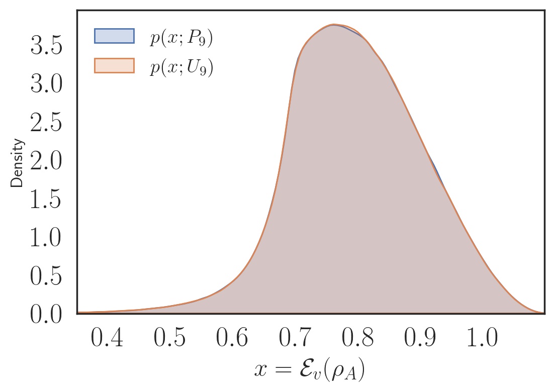
Figure 7: Two-qutrit case, $d^{2}=9$. Distributions $p(x;U)$ of entanglement obtained from the action of $9\times 9$ unitaries $U$ on Haar distributed product states. Shown are two distributions, one corresponding to the 2-unitary permutation matrix $P_{9}$, Eq. (80) and other a 2-unitary $U_{9}$ obtained from the map with a random seed. These two are numerically indistinguishable, and we could not find a different distribution than the one shown here for $O(10^{3})$ number of 2-unitaries obtained from the map.

Surprisingly, both the distributions are indistinguishable for these 2-unitaries, although their origins and forms are very different. We have checked entanglement distributions for $O(10^{3})$ 2-unitaries obtained from the map but could not find a different distribution from that of the 2-unitary permutation matrix. In fact in most cases we could transform 2-unitaries obtained from the map, using random seeds, into 2-unitary permutation matrices using appropriate local transformations in $\mathcal{U}(3)\otimes\mathcal{U}(3)$. Based on overwhelming numerical evidence we propose the following conjecture:

Conjecture 1.

All 2-unitaries of order 9 are LU equivalent to $P_{9}$.

VI.3 2-unitaries in $d=4$

VI.3.1 Permutations

The total number of 2-unitary permutations of size $16$ is $2\times 3456=6912$. By performing a direct exhaustive search over local permutations, quite remarkably even in this case it turns out that all $6912$ 2-unitary permutations are LU equivalent and thus lead to the following proposition.

Proposition 3.

There is only one LU class of 2-unitary permutations of order 16.

We choose the following 2-unitary permutation matrix as a representative of the LU equivalent class of 2-unitary permutations of order 16,

$$P_{16}=\begin{pmatrix}\begin{array}[]{cccc|cccc|cccc|cccc}1&.&.&.&.&.&.&.&.&.&.&.&.&.&.&.\\ .&.&.&.&.&1&.&.&.&.&.&.&.&.&.&.\\ .&.&.&.&.&.&.&.&.&.&1&.&.&.&.&.\\ .&.&.&.&.&.&.&.&.&.&.&.&.&.&.&1\\ \hline\cr.&.&.&.&.&.&.&1&.&.&.&.&.&.&.&.\\ .&.&1&.&.&.&.&.&.&.&.&.&.&.&.&.\\ .&.&.&.&.&.&.&.&.&.&.&.&.&1&.&.\\ .&.&.&.&.&.&.&.&1&.&.&.&.&.&.&.\\ \hline\cr.&.&.&.&.&.&.&.&.&1&.&.&.&.&.&.\\ .&.&.&.&.&.&.&.&.&.&.&.&1&.&.&.\\ .&.&.&1&.&.&.&.&.&.&.&.&.&.&.&.\\ .&.&.&.&.&.&1&.&.&.&.&.&.&.&.&.\\ \hline\cr.&.&.&.&.&.&.&.&.&.&.&.&.&.&1&.\\ .&.&.&.&.&.&.&.&.&.&.&1&.&.&.&.\\ .&.&.&.&1&.&.&.&.&.&.&.&.&.&.&.\\ .&1&.&.&.&.&.&.&.&.&.&.&.&.&.&.\end{array}\end{pmatrix}$$ (82)

Using $(4!)^{4}=3,31,776$ possible local permutations, each 2-unitary permutation is obtained $48$ times and therefore all $3,31,776/48=6912$ are taken into account.

VI.3.2 Entangled OLS of size $4$: A new example of AME($4,4$)

Although there is only one LU class of 2-unitary permutations of order 16, we give an explict example of a 2-unitary orthogonal matrix which is not LU equivalent to any 2-unitary permutation. This is obtained via the nonlinear map $\mathcal{M}_{\Gamma R}$ given in Eq. (23) with a permutation seed, and is given by

$$O_{16}=\frac{1}{2}\begin{pmatrix}\begin{array}[]{cccc|cccc|cccc|cccc}1&.&.&.&.&1&.&.&.&.&-1&.&.&.&.&-1\\ .&1&.&.&-1&.&.&.&.&.&.&-1&.&.&-1&.\\ .&.&-1&.&.&.&.&1&-1&.&.&.&.&-1&.&.\\ .&.&.&-1&.&.&1&.&.&1&.&.&1&.&.&.\\ \hline\cr.&1&.&.&-1&.&.&.&.&.&.&1&.&.&1&.\\ -1&.&.&.&.&1&.&.&.&.&1&.&.&.&.&-1\\ .&.&.&-1&.&.&1&.&.&-1&.&.&-1&.&.&.\\ .&.&-1&.&.&.&.&-1&1&.&.&.&.&-1&.&.\\ \hline\cr.&.&-1&.&.&.&.&-1&-1&.&.&.&.&1&.&.\\ .&.&.&1&.&.&1&.&.&-1&.&.&1&.&.&.\\ -1&.&.&.&.&-1&.&.&.&.&-1&.&.&.&.&-1\\ .&-1&.&.&-1&.&.&.&.&.&.&-1&.&.&1&.\\ \hline\cr.&.&.&-1&.&.&-1&.&.&-1&.&.&1&.&.&.\\ .&.&1&.&.&.&.&-1&-1&.&.&.&.&-1&.&.\\ .&1&.&.&1&.&.&.&.&.&.&-1&.&.&1&.\\ 1&.&.&.&.&-1&.&.&.&.&1&.&.&.&.&-1\end{array}\end{pmatrix}$$ (83)

This matrix can be written in a compact form as

$$O_{16}=P_{16}^{T}D_{4}P_{16},$$ (84)

where $D_{4}$ is a block-diagonal matrix consisting of four $4\times 4$ Hadamard matrices. Each row or column of $O_{16}$ contains four non-zero entries being equal to either $1/2$ or, $-1/2$ and is such that its eighth power is equal to the Identity, $O_{16}^{8}=\mathbb{I}$. To show that $O_{16}$ is indeed not LU equivalent to $P_{16}$, we compare the entanglement distributions $p(x;O_{16})$ and $p(x;P_{16})$. The distributions, shown in Fig. (8) are clearly distinguishable, $p(x;O_{16})\neq p(x;P_{16})$ and thus $O_{16}\stackrel{{\scriptstyle LU}}{{\nsim}}P_{16}$. Entanglement distributions for a large number of generic 2-unitaries obtained by applying the dynamical map $\mathcal{M}_{\Gamma R}$ on random seed unitaries did not result in any other distinguishable distributions other than the ones shown in Fig. (8). This suggests that there are at least three LU classes of 2-unitaries in $d^{2}=16$. The representatives of these 3 LU classes are: (i) $P_{16}$ given by Eq. (82), (ii) enphased $P_{16}$; $P_{16}^{{}^{\prime}}=D_{1}\,P_{16}\,D_{2}$, where $D_{1}$ and $D_{2}$ are diagonal unitaries with arbitrary phases, and (iii) $O_{16}$ given by Eq. (83). Note that $P_{16}$ and $P_{16}^{{}^{\prime}}$ are not LU equivalent in general and thus the corresponding AME states of minimal support are not LU equivalent.

Each row or, column of $O_{16}$ treated as a pure state in $\mathcal{H}_{4}\otimes\mathcal{H}_{4}$ is maximally entangled and thus the underlying combinatorial design corresponding to $O_{16}$ does not factor into separable structures $\mathcal{K}$ and $\mathcal{L}$ defined in Eq. (69). Also note that each $4\times 4$ block in Eq. (83) is unitary up to a scale factor and thus rows or columns of $O_{16}^{R}$ are also maximally entangled states in $\mathcal{H}_{4}\otimes\mathcal{H}_{4}$. Similar entangled combinatorial structure corresponding to 2-unitary of size $36$ has been referred to as entangled orthogonal quantum Latin squares (OQLS) in Ref. Rather et al. (2022) in which entangled OQLS of size six was found. Based on our discussion in previous section on 2-unitaries of size $9$ and the known fact that there are no 2-unitaries of size $4$, $d=4$ seems to be the smallest possible dimension in which entangled OLS exists.

This allows us to construct a new kind of AME state of four ququads; AME($4,4$), which is not LU equivalent to AME state of minimal support constructed from $P_{16}$. The corresponding AME state written in computational basis is given by,

$$\ket{\text{AME}(4,4)}=\sum_{i,j,k,l=1}^{4}(O_{16})_{ij,kl}\ket{ijkl}.$$ (85)

The tensor $T_{ijkl}=(O_{16})_{ij,kl}$ is a perfect tensor Pastawski et al. (2015) whose non-zero entries are given by Eq. (83). To our knowledge this is the simplest AME state that is not derived from a classical design or is equivalent to one, for equivalence among AME states, see for example Burchardt and Raissi (2020); Raissi et al. (2020). Thus it qualifies as a younger cousin of the AME(4,6) which is a genuine quantum orthogonal Latin square Rather et al. (2022). However, unlike the golden state AME(4,6), this is purely real. Earlier constructions of ququad AME states have much larger number of particles Raissi et al. (2020).

We performed several local unitary transformations on $O_{16}$ and reduced the numer of it’s non-zero entries or, equivalently the support of AME state given by Eq. (85), from $64$ to $42$, although the transformed matrix has entries other than $\pm 1/2$. The transformed matrix has two unentangled columns and theferore $O_{16}$ is not a universal entangler.

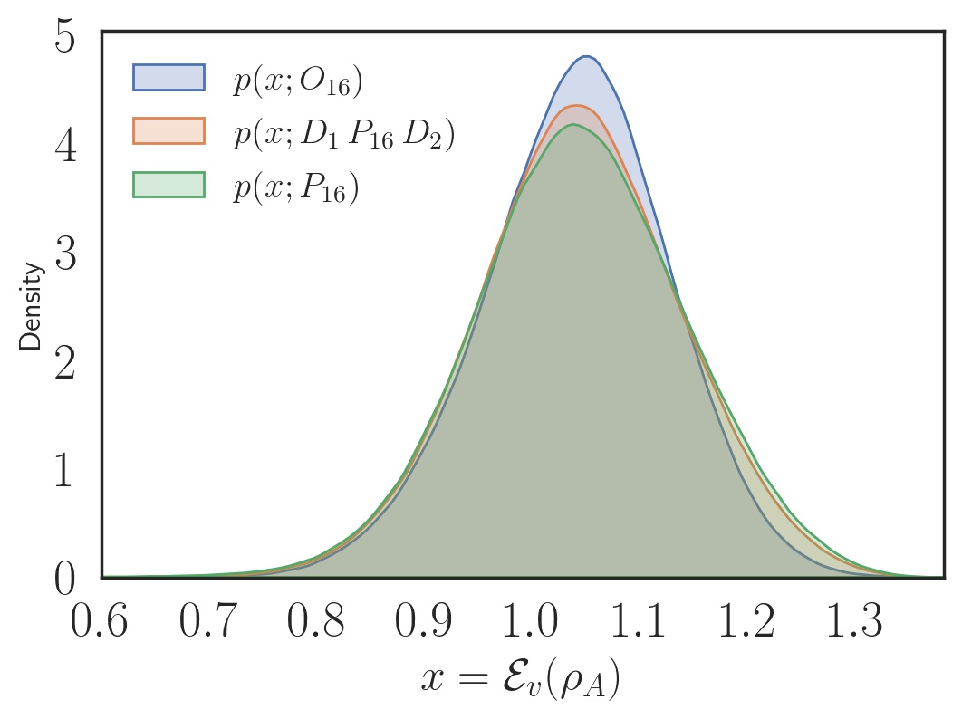
Figure 8: Two-ququad case, $d^{2}=16$. Distributions $p(x;U)$ of entanglement corresponding to 2-unitary permutation matrix $U=P_{16}$ (Eq. (82)) and the 2-unitary orthogonal matrix $U=O_{16}$ (Eq. (83)). The distributions are clearly distinguishable and shows that $P_{16}$ and $O_{16}$ are not LU equivalent. Shown also is the entanglement distribution corresponding to enphased $P_{16}$; $D_{1}P_{16}D_{2}$ where $D_{1}$ and $D_{2}$ are diagonal unitaries, which is not LU equivalent to either $P_{16}$ or $O_{16}$.

VII Entangling properties of dual and T-dual permutation matrices

Permutation matrices form an important class of entangling unitary operators Clarisse et al. (2005). In this section we study the entangling properties of dual and T-dual permutation matrices on $\mathcal{H}_{d}\otimes\mathcal{H}_{d}$ which are special subsets of the permutation group $\mathrm{P}(d^{2})$. Dual unitary permutation matrices have been recently explored in Borsi and Pozsgay (2022) and used as building blocks of quantum circuits with interesting dynamical behaviour Aravinda et al. (2021). Two permutation matrices $P_{1}$ and $P_{2}$ have been defined in Clarisse et al. (2005) to belong to the same entangling class if they have the same entangling power, $e_{p}(P_{1})=e_{p}(P_{2})$. Two LU equivalent permutation matrices always belong to the same entangling class but permutation matrices belonging to the same entangling power need not be LU equivalent. For the sake of convenience we write the permutation matrix in terms of the column number of the only non-zero entry in each row. For example in this notation $P_{9}$ given by Eq. (80) is written as $P_{9}=\left\{1,5,9,6,7,2,8,3,4\right\}$ corresponding to the permutation, $\pi:\left\{1,2,3,4,5,6,7,8,9\right\}\rightarrow\left\{\pi(1)=1,\pi(2)=5,\cdots,\pi(8)=3,\pi(9)=4\right\}.$

VII.1 Dual-unitary and T-dual permutations in $d=2$ and $d=3$

We list all possible entangling classes for dual-unitary permutations in $\mathrm{P}(d^{2})$ for $d=2,3$.

Two-qubit case: In this case the corresponding permutation group is $\mathrm{P}(4)$. The projection of $\mathrm{P}(4)$ on $e_{p}$-$g_{t}$ plane is shown in Fig. (9). There are $4$ distinct points corresponding to $24$ possible permutations of order $4$, treated as two-qubit gates, on the $e_{p}$-$g_{t}$ plane and every permutation matrix is either dual or T-dual. Number of entangling classes is only $2$ which are listed in Table 2.

Table 2: Entangling and LU classes of dual (equivalently T-dual) permutations in $\mathrm{P}(4)$.

S.No.	$e_{p}(P)$	# LU classes
1	0	1
2	$\frac{2}{3}$	1

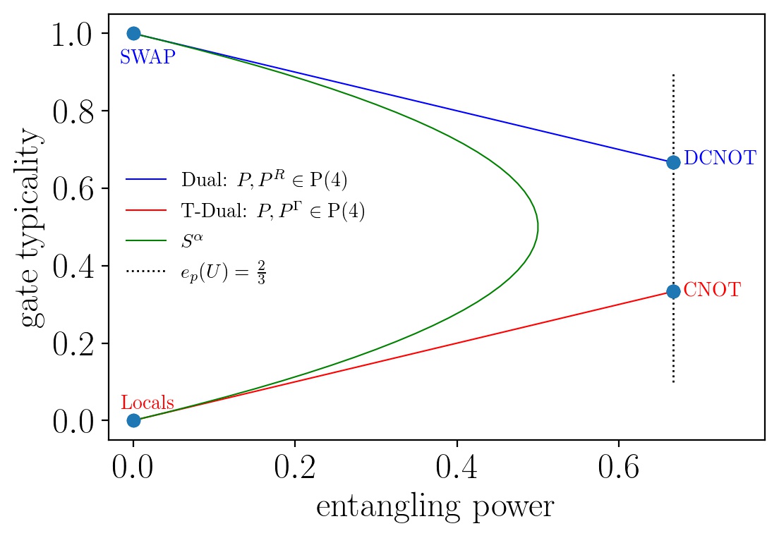
Figure 9: Two-qubit case, $d^{2}=4$. The entangling power vs gate-typicality, of all permutations $\mathrm{P}(4)$, treated as two-qubit gates. Number of entangling classes, those with different entangling powers, is $2$.

Two-qutrit case: In this case the corresponding permutation group is $\mathrm{P}(9)$. The projection of $\mathrm{P}(9)$, treated as two-qutrit gates, on the $e_{p}$-$g_{t}$ plane is shown in Fig. (10). There are only $60$ distinct points on the $e_{p}$-$g_{t}$ plane from the $9!=3,62,000$ possible permutation matrices of order $9$.

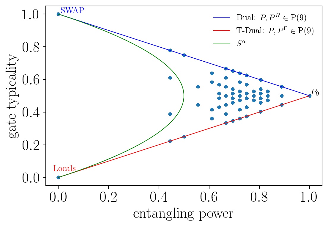
Figure 10: Two-qutrit case, $d^{2}=9$. The entangling power vs gate-typicality, of all $9!$ permutations $\mathrm{P}(9)$, treated as two-qutrit gates. Number of entangling classes corresponding to dual (and equivalently T-dual) permutation matrices is $10$.

It was shown in Ref. Krishnan and Sunder (1996) that there are 18 LU classes of T-dual (or equivalently dual-unitary) permutation matrices. A representative permutation from each LU class are also listed therein. These LU classes are listed in the Table 3 along with their entangling powers. Therefore the number of entangling classes corresponding to dual unitary (and equivalently T-dual) permutation matrices is $10$.

Except for 3 entangling classes (corresponding to $e_{p}(P)=0,\,8/9,$ and $1$), there are more than one LU classes. Taking permutations from two different LU classes with the same entangling power (say $e_{p}(P)=1/2$), we observed that these produce the same entanglement distributions $p(x;U)$. This suggests that these LU inequivalent permutations with the same entangling power and gate-typicality might be connected by the swap gate. Indeed we found that according to the LUS classification defined in Eq. (79) with $a=b=1$ that there are only $11$ LUS classes i.e., two permutations $P$ and $P^{\prime}$ belonging to the same entangling class but different LU classes are related (up to local permutations) as $P^{\prime}=SPS$, where $S$ is the swap gate. This is the case for all entangling classes in the Table 3 with more than one LU classes except for the entangling class $e_{p}(U)=2/3$.

Table 3: Entangling, LU and LUS classes of dual (equivalently T-dual) permutations in $\mathrm{P}(9)$.

S.No.	$e_{p}(P)$	# LU classes	# LUS classes
1	0	1	1
2	$\frac{4}{9}$	2	1
3	$\frac{1}{2}$	2	1
4	$\frac{2}{3}$	3	2
5	$\frac{25}{36}$	2	1
6	$\frac{13}{18}$	2	1
7	$\frac{3}{4}$	2	1
8	$\frac{29}{36}$	2	1
9	$\frac{8}{9}$	1	1
10	1	1	1
Total		18	11

The entangling class $e_{p}(U)=2/3$ is special and has two LUS classes. Representative permutations written in compact form as $P=\left\{1,4,8,2,5,7,6,3,9\right\}$ and $P^{\prime}=\left\{1,4,9,2,5,8,6,3,7\right\}$ from both LUS classes produce distinguishable entanglement distributions shown in Fig. (11). The LU inequivalence between $P$ and $P^{\prime}$ can also be seen via the singular values of $P^{\Gamma}$ and $P^{{}^{\prime}\Gamma}$ which are LUI’s (see Eq. (17)); singular values of $P^{\Gamma}$ and $P^{{}^{\prime}\Gamma}$ are $\left\{2,2,1\right\}$ and $\left\{\sqrt{5},\sqrt{2},\sqrt{2}\right\}$ respectively. This leads us to the strong suspicion that the equality of entanglement distributions may be a sufficient condition for LUS equivalence, i.e., $p(x;U)=p(x;U^{\prime})$ iff $U\stackrel{{\scriptstyle LUS}}{{\sim}}U^{\prime}$.

An interesting fact we observed is that with von Neumann entropy as a measure of entanglement the average of distributions obtained for these permutations differ slightly; for $P$, $\overline{\mathcal{E}_{v}(\rho_{A})}\approx 0.57$ while for $P^{\prime}$ $\overline{\mathcal{E}_{v}(\rho_{A})}\approx 0.55$, taking into acccount $10^{6}$ realisations of product states in both cases. Note that if the linear entropy is taken as a measure then the averages must be equal according to the definition of the entangling power Zanardi (2001). This suggests the role of other unknown LU invariants besides $E(U)$ and $E(US)$ which determine the average of the entanglement distribution when von Neumann entropy is taken as a measure of entanglement.

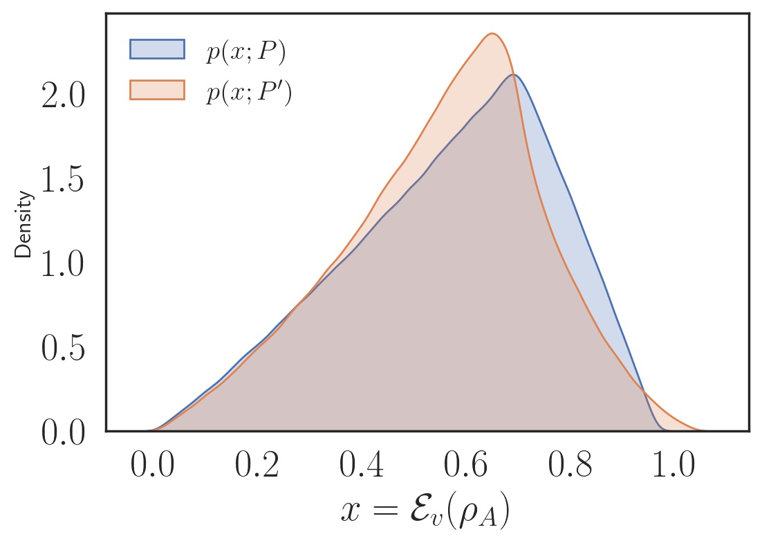
Figure 11: Entanglement distributions obtained for $P$ and $P^{\prime}$ permutation matrices of size $9$ belonging to two LUS classes, see text, corresponding to the entangling class with $e_{p}(U)=2/3$. Distinguishabiliity of the distributions imply that $P$ and $P^{\prime}$ are not LU equivalent.

It is to be noted that out of 18 possible LU classes only one corresponds to the entangling class $e_{p}(P)=1$ of 2-unitary permutations. As a consequence of this all 72 possible 2-unitary permutations of order $9$ are locally equivalent consistent with Proposition 2.

VII.2 Numerical results for $d>3$

Total possible number of LU classes of dual or, T-dual permutations in $\mathrm{P}(d^{2})$ for $d>3$ is not known. The number of entangling classes is also not known, as an exhaustive enumeration of such permuatations is prohibitively large. To get a lower bound on the possible number of entangling classes corresponding to dual-unitary permutations of size 16 we numerically search over permutations in the vicinity of different permutations like swap and 2-unitary gates. Results obtained from such a search over around $1.2\times 10^{7}$ permutations of size $16$ (out of a possible $16!\sim 10^{13}$) is shown in Fig. (12). We obtain $56$ entangling classes corresponding to dual or equivalently T-dual permutations. This provides a weak lower bound on the number of LU inequivalent classes for dual-unitary permutations of size $16$. Note that one of the entangling classes is $e_{p}(U)=1$ corresponding to 2-unitary permutations for which there is only one LU equivalence class (see Proposition 3).

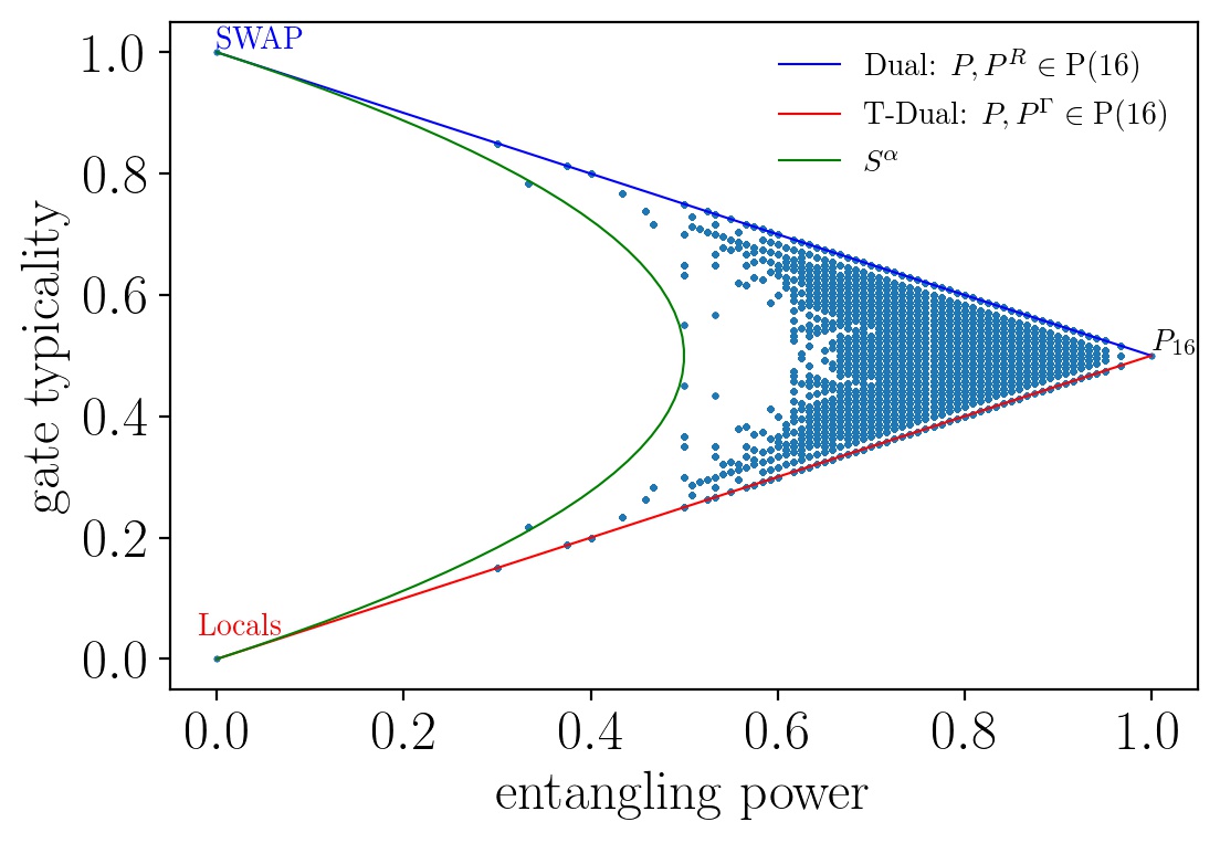
Figure 12: Two-ququad case, $d^{2}=16$. The entangling power vs gate-typicality of $1.2\times 10^{7}$ permutations (out of total $16!\approx 10^{13}$ permutations), treated as two-ququad gates. Number of entangling classes corresponding to dual (and equivalently T-dual) permutation matrices obtained from our numerical search is found to be $56$.

We end this section by showing that there exist more than one LU classes for 2-unitary permutations in $d>4$. An easy way to see this is by comparing entanglement distributions of 2-unitary permutation $P\in\mathrm{P}(d^{2})$ and its realignment $P^{R}\in\mathrm{P}(d^{2})$. This is shown in Fig. (13) for a 2-unitary permutation in $d=5$ given by

$$\begin{split}P_{25}&=\left\{1,7,13,19,25,22,3,9,15,16,18,24,5,6,12,14,20,21,2,8,10,11,17,23,4\right\},\\ P_{25}^{R}&=\left\{1,7,13,19,25,8,14,20,21,2,15,16,22,3,9,17,23,4,10,11,24,5,6,12,18\right\}.\end{split}$$ (86)

Entanglement distributions are different; $p(x;P_{25})\neq p(x;P_{25}^{R})$ and thus establishes that they are not LU equivalent. Recall that one can cannot jusify LU inequivalence between 2-unitaries based on the singular values of their reshuffled and partially transposed rearrangements as they are all maximized being equal to $1$. We checked entanglement distributions for $100$ 2-unitary permutations of size $25$ together with their different rearrangements but found only two different distributions shown in Fig. (13). Thus total number of LU and LUS classes for 2-unitary permutations in $d=5$ remains unknown but it is certainly greater than $1$. Similarly in $d=7,8,$ and $9$ we observed only two different distributions corresponding to 2-unitary permutations and their rearrangements.

A consequence of having more than one LU classes of 2-unitary permutations in $d>3$ results in minimal support AME states which are not LU equivalent. Our results thus contradict the Conjecture 2 in Ref. Burchardt and Raissi (2020) which in particular for four party states implies that there is only one LU class of AME states of minimal support. As we have illustrated in Fig. (8) and Fig. (13) there exist more than one LU classes of AME states of minimal support for $d=4$ and $5$.

Assuming that 2-unitary permutations belonging to the same LU class are always related by local permutations one can argue that there are more than one LU classes of 2-unitary permutations for $d=7,8,$ and $9$ as the number of possible orthogonal Latin squares (see A072377 , Ref. Sloane and Inc. (2020)) exceeds $(d!)^{4}$ number of orthogonal Latin squares obtained from 2-unitary permutation $P$ using local permutations $p_{i}$’s of size $d$ on both sides; $(p_{1}\otimes p_{2})P(p_{3}\otimes p_{4})$. Note that all $(d!)^{4}$ number of orthogonal Latin squares so obtained are not all different but even with redundancy this is less than the number of possible orthogonal Latin squares in $d>5$. Interestingly in $d=5$ we found that although $(d!)^{4}$ exceeds the number of possible orthogonal Latin squares but it is not a factor of it which is the case for $d=3$ and $4$.

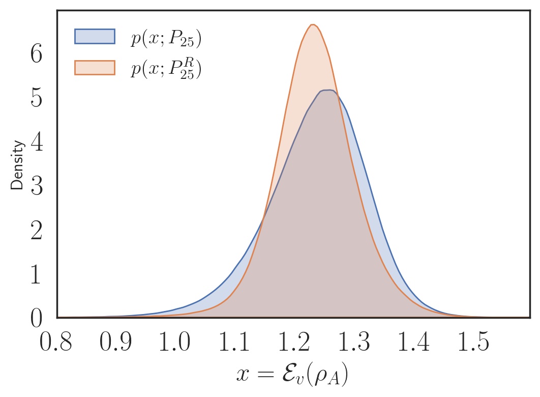
Figure 13: $d^{2}=25$. Entanglement distributions of 2-unitary permutation $P_{25}$, Eq. (86), and it’s realignment $P_{25}^{R}$ which is also a 2-unitary. The distributions are clearly distinguishable; $p(x;P_{25})\neq p(x;P_{25}^{R})$, and thus shows that $P_{25}\stackrel{{\scriptstyle LU}}{{\nsim}}P_{25}^{R}$.

VIII Summary and discussions

Despite several constructions of the set of dual-unitary operators, the complete characterization for arbitrary local Hilbert space dimension remains an open problem. In Ref. Rather et al. (2020), we proposed a non-linear iterative map that produces dual-unitary operators from arbitrary seed unitaries. The map acts as a dynamical system in the space of bipartite unitary operators. In this work, we have studied the period-two fixed points of the map which are dual-unitary operators and provided a stochastic generalization of the map which produces structured fixed points which are dual unitaries. Complete characterization of the fixed points of all orders remains to be understood and makes the map a novel dynamical system in its own right. For two-qubit gates, using the canonical or Cartan decomposition we analytically study the convergence rates for various initial conditions. However, convergence of the map in local Hilbert space dimension $d>2$ remains an unsolved problem.

The subset of dual-unitary operators having maximum entangling power is that of 2-unitary operators. The 2-unitary permutation operators can be constructed from combinatorial designs called orthogonal Latin squares (OLS). The non-existence of OLS of size 6 motivates to look for general quantum combinatorial designs corresponding to 2-unitary operators as was recently found in Ref. Rather et al. (2022) for local dimension $d=6$. The problem of finding such quantum combinatorial designs reduces to finding the 2-unitary operators which are not LU equivalent to any 2-unitary permutation matrix. From our extensive numerical searches using the dynamical map and known constructions of 2-unitaries, we could not find any such quantum design for local dimension $d=3$. All 2-unitary permutation operators of size $9$ are local unitarily (LU) equivalent to each other. Based on these results we conjecture that all 2-unitary operators of size $9$, not just permutations, are LU equivalent to each other. If true, this implies that there is just one 2-unitary two-qutrit gate up to LU equivalence.

Methods to ascertain local unitary (LU) equivalence between bipartite unitary operators is not known in general. For unitary operators with identical values of known local unitary invariants (LUI’s) like the entangling power and the gate-typicality, the problem of LU equivalence becomes harder. In this paper we have proposed a necessary criterion for distinguishing LU inequivalent 2-unitary operators based on the entanglement distribution these produce. Using the iterative map we found a 2-unitary operator for local dimension $d=4$ which is LU inequivalent to any 2-unitary permutation of the same size. Thus this qualifies as a genuine 2-unitary quantum design in the lowest possible dimension, as they do not exist for $d=2$ and as far as we know, for $d=3$. This also implies that we have displayed an explicit example of an AME($4,4$) state that is not LU equivalent to AME($4,4$) of minimal support. We have shown that for $d=5$ there are at least two LU classes of 2-unitary permutations and thus there are two LU inequivalent AME states of minimal support. Consequences of these new examples of AME states for quantum error-correction is an interesting direction and is left for future studies. Stochastic local operations and classical communication (SLOCC) equivalence of LU inequivalent four party AME states found in this work for $d>3$ is an interesting problem and is left for future studies.

Note: After this paper was written, we came to know of Ref. Kodiyalam and Sunder (2004) wherein a criterion for determining local unitary equivalence of operators is presented that involves an exponential (in local dimension) set of invariants.

Appendix A Details about the map in the two-qubit case

In the two-qubit case, the Cartan form of any unitary (27) can be written as

$$U_{0}=\left(\begin{array}[]{cccc}e^{-ic_{3}^{(0)}}c_{-}^{(0)}&0&0&-ie^{-ic_{3}^{(0)}}s_{-}^{(0)}\\ 0&e^{ic_{3}^{(0)}}c_{+}^{(0)}&-ie^{ic_{3}^{(0)}}s_{+}^{(0)}&0\\ 0&-ie^{ic_{3}^{(0)}}s_{+}^{(0)}&e^{ic_{3}^{(0)}}c_{+}^{(0)}&0\\ -ie^{-ic_{3}^{(0)}}s_{-}^{(0)}&0&0&e^{-ic_{3}^{(0)}}c_{-}^{(0)}\end{array}\right)$$ (87)

where,

$$c_{\pm}^{(0)}=\cos(c_{1}^{(0)}\pm c_{2}^{(0)});\qquad s_{\pm}^{(0)}=\sin(c_{1}^{(0)}\pm c_{2}^{(0)}).$$

The unitary operator $U$ in its canonical decomposition has four parameters. Let $\alpha_{0}=e^{-ic_{3}^{(0)}}c_{-}^{(0)},\beta_{0}=-ie^{-ic_{3}^{(0)}}s_{-}^{(0)},\gamma_{0}=-ie^{ic_{3}^{(0)}}s_{+}^{(0)},$ and $\delta_{0}=e^{ic_{3}^{(0)}}c_{+}^{(0)}$. Then the Eq. (87) can be written as

$$U_{0}=\left(\begin{array}[]{cccc}\alpha_{0}&0&0&\beta_{0}\\ 0&\delta_{0}&\gamma_{0}&0\\ 0&\gamma_{0}&\delta_{0}&0\\ \beta_{0}&0&0&\alpha_{0}\end{array}\right).$$ (88)

The $\mathcal{M}_{R}$ map can now be studied analytically by applying it to the two qubit unitary operators in its Cartan form (88). Action of linear map $R$ on $U_{0}$ defined in Eq. (88) results

$$U^{R}_{0}=\left(\begin{array}[]{cccc}\alpha_{0}&0&0&\delta_{0}\\ 0&\beta_{0}&\gamma_{0}&0\\ 0&\gamma_{0}&\beta_{0}&0\\ \delta_{0}&0&0&\alpha_{0}\end{array}\right).$$ (89)

The polar decomposition of the matrix $U_{0}^{R}$, which is given by $U_{0}^{R}=U_{1}H$, where $U_{1}$ is unitary and $H=\sqrt{U^{R\dagger}U^{R}}$ is given by

$$H=\frac{1}{2}\left(\begin{array}[]{cccc}|\alpha_{0}-\delta_{0}|+|\alpha_{0}+\delta_{0}|&0&0&-|\alpha_{0}-\delta_{0}|+|\alpha_{0}+\delta_{0}|\\ 0&|\beta_{0}-\gamma_{0}|+|\beta_{0}+\gamma_{0}|&-|\beta_{0}-\gamma_{0}|+|\beta_{0}+\gamma_{0}|&0\\ 0&-|\beta_{0}-\gamma_{0}|+|\beta_{0}+\gamma_{0}|&|\beta_{0}-\gamma_{0}|+|\beta_{0}+\gamma_{0}|&0\\ -|\alpha_{0}-\delta_{0}|+|\alpha_{0}+\delta_{0}|&0&0&|\alpha_{0}-\delta_{0}|+|\alpha_{0}+\delta_{0}|\end{array}\right).$$ (90)

The unitary $U_{1}=U_{0}^{R}H^{-1}$ is given by

$$U_{1}=\left(\begin{array}[]{cccc}\alpha_{0}\alpha_{+}+\delta_{0}\alpha_{-}&0&0&\alpha_{0}\alpha_{-}+\delta_{0}\alpha_{+}\\ 0&\beta_{0}\beta_{+}+\gamma_{0}\beta_{-}&\beta_{0}\beta_{-}+\gamma_{0}\beta_{+}&0\\ 0&\gamma_{0}\beta_{+}+\beta_{0}\beta_{-}&\gamma_{0}\beta_{-}+\beta_{0}\beta_{+}&0\\ \alpha_{0}\alpha_{-}+\delta_{0}\alpha_{+}&0&0&\alpha_{0}\alpha_{+}+\delta_{0}\alpha_{-}\end{array}\right),$$ (91)

where $\alpha_{\pm}$ and $\beta_{\pm}$ are given as

$$\begin{split}\alpha_{\pm}&=\frac{|\alpha_{0}-\delta_{0}|\pm|\alpha_{0}+\delta_{0}|}{2|\alpha_{0}-\delta_{0}||\alpha_{0}+\delta_{0}|}\\ \beta_{\pm}&=\frac{|\beta_{0}-\gamma_{0}|\pm|\beta_{0}+\gamma_{0}|}{2|\beta_{0}-\gamma_{0}||\beta_{0}+\gamma_{0}|}\end{split}$$ (92)

Note that although $U_{0}\in\mathcal{SU}(4)$ but $U_{1}$ given by Eq. (91) need not be in $\mathcal{SU}(4)$ in general. The mapping between $\alpha_{0},\beta_{0},\gamma_{0},\delta_{0}$ of $U_{0}$ and $\alpha_{1}^{\prime},\beta_{1}^{\prime},\gamma_{1}^{\prime},\delta_{1}^{\prime}$ of $U_{1}$ is

$$\alpha_{1}^{\prime} =\frac{(\alpha_{0}+\delta_{0})|\alpha_{0}-\delta_{0}|+(\alpha_{0}-\delta_{0})|\alpha_{0}+\delta_{0}|}{2|\alpha_{0}-\delta_{0}||\alpha_{0}+\delta_{0}|}$$

$$\beta_{1}^{\prime} =\frac{(\alpha_{0}+\delta_{0})|\alpha_{0}-\delta_{0}|-(\alpha_{0}-\delta_{0})|\alpha_{0}+\delta_{0}|}{2|\alpha_{0}-\delta_{0}||\alpha_{0}+\delta_{0}|}$$

$$\gamma_{1}^{\prime} =\frac{(\beta_{0}+\gamma_{0})|\beta_{0}-\gamma_{0}|-(\beta_{0}-\gamma_{0})|\beta_{0}+\gamma_{0}|}{2|\beta_{0}-\gamma_{0}||\beta_{0}+\gamma_{0}|}$$

$$\delta_{1}^{\prime} =\frac{(\beta_{0}+\gamma_{0})|\beta_{0}-\gamma_{0}|+(\beta_{0}-\gamma_{0})|\beta_{0}+\gamma_{0}|}{2|\beta_{0}-\gamma_{0}||\beta_{0}+\gamma_{0}|}.$$ (93)

The above set of equations written in a compact form as

$$\begin{pmatrix}\alpha_{1}^{\prime}\\ \beta_{1}^{\prime}\\ \gamma_{1}^{\prime}\\ \delta_{1}^{\prime}\end{pmatrix}=\begin{pmatrix}\alpha_{+}&0&0&\alpha_{-}\\ \alpha_{-}&0&0&\alpha_{+}\\ 0&\beta_{-}&\beta_{+}&0\\ 0&\beta_{+}&\beta_{-}&0\end{pmatrix}\begin{pmatrix}\alpha_{0}\\ \beta_{0}\\ \gamma_{0}\\ \delta_{0}\end{pmatrix},$$ (94)

depicts the non-linear nature of the map.

Appendix B Proofs of the fixed point theorems in the two-qubit case

B.1 Proof of Theorem 1

Proof.

Let $U_{0}$ be a two-qubit gate of the form Eq. (35). If $U_{0}$ is fixed point of the $\mathcal{M}_{R}$ map:

$$\mathcal{M}_{R}[U_{0}]=U_{1}=U_{0}.$$ (95)

As this implies that $U_{1}$ is also in $\mathcal{SU}(4)$, $\chi_{1}=0$. Using Eq. (37), the fixed point condition $\mathcal{M}_{R}[U_{0}]=U_{0}$ can be written as

$$\alpha_{0} =\frac{1}{2}[(k_{+}^{(0)}+k_{-}^{(0)})\alpha_{0}+(k_{+}^{(0)}-k_{-}^{(0)})\delta_{0}],$$ (96a)

$$\beta_{0} =\frac{1}{2}[(k_{+}^{(0)}-k_{-}^{(0)})\alpha_{0}+(k_{+}^{(0)}+k_{-}^{(0)})\delta_{0}],$$ (96b)

$$\gamma_{0} =\frac{1}{2}[(l_{+}^{(0)}-l_{-}^{(0)})\beta_{0}+(l_{+}^{(0)}+l_{-}^{(0)})\gamma_{0}],$$ (96c)

$$\delta_{0} =\frac{1}{2}[(l_{+}^{(0)}+l_{-}^{(0)})\beta_{0}+(l_{+}^{(0)}-l_{-}^{(0)})\gamma_{0}],$$ (96d)

where $k_{\pm}^{(0)}=1/|\alpha_{0}\pm\delta_{0}|$ and $l_{\pm}^{(0)}=1/|\beta_{0}\pm\gamma_{0}|$. From the unitarity of $U_{0}$, it follows that Re$(\alpha_{0}\beta_{0}^{*})=$Re$(\gamma_{0}\delta_{0}^{*})=0$. Multiplying Eq. (96a) by $\gamma_{0}^{*}$, Eq. (96c) by $\alpha_{0}^{*}$ in Eq. (96) and taking real parts one obtains $k_{+}^{(0)}+k_{+}^{(0)}=l_{+}^{(0)}+l_{+}^{(0)}=2$. Similarly, multiplying Eq. (96a) by $\beta_{0}^{*}$ and taking the real parts we get

$$(k_{+}^{(0)}-k_{-}^{(0)})\text{Re}[\delta_{0}\beta_{0}^{*}]=0.$$ (97)

Therefore, either $k_{+}^{(0)}=k_{-}^{(0)}$ or Re$[\delta_{0}\beta_{0}^{*}]=0$. For $k_{+}^{(0)}=k_{-}^{(0)}$ together with the condition $k_{+}^{(0)}+k_{+}^{(0)}=2$, from Eq. (96b), it follows that $\beta_{0}=\delta_{0}$. For $U_{0}$ with $\beta_{0}=\delta_{0}\neq 0$, it is can be shown that $\gamma_{0}=\pm\alpha_{0}$ using the unitarity of $U_{0}$. Therefore, $U_{0}$ is of the form

$$U_{0}=\left(\begin{array}[]{cccc}\alpha_{0}&0&0&\beta_{0}\\ 0&\beta_{0}&\pm\alpha_{0}&0\\ 0&\pm\alpha_{0}&\beta_{0}&0\\ \beta_{0}&0&0&\alpha_{0}\end{array}\right)\;,$$ (98)

which satisfies $U_{0}^{R}=U_{0}$ and thus is a self-dual unitary. From Eq. (96b) and Eq. (96d) using unitarity of $U_{0}$ together with $k_{+}^{(0)}+k_{+}^{(0)}=l_{+}^{(0)}+l_{+}^{(0)}=2$, it follows that $|\beta_{0}|^{2}=|\delta_{0}|^{2}=$ Re$(\beta_{0}\delta_{0}^{*})$. Therefore, the other condition Re$(\beta_{0}\delta_{0}^{*})=0$ in Eq. (97) is satisfied only when $\beta_{0}=\delta_{0}=0$. In this case $U_{0}$ is of the form

$$U_{0}=\left(\begin{array}[]{cccc}\alpha_{0}&0&0&0\\ 0&0&\gamma_{0}&0\\ 0&\gamma_{0}&0&0\\ 0&0&0&\alpha_{0}\end{array}\right)\;,$$ (99)

where $|\alpha_{0}|=|\gamma_{0}|=1$ and is also self-dual unitary. Hence, all period-one fixed points of the $\mathcal{M}_{R}$ map in the two-qubit case are self-dual. ∎

Canonical form of the dual-unitaries obtained by setting $c_{1}=c_{2}=\pi/4$ in Eq. (87) is of the form Eq. (99). Self-dual unitaries of the form Eq. (98) are LU equivalent to the canonical form. For example, $(H\otimes H)U_{0}(H\otimes H)$, $H$ being the Hadamard gate; $H=\frac{1}{\sqrt{2}}\begin{pmatrix}1&1\\ 1&-1\end{pmatrix}$, is of the canonical form where $U_{0}$ is of the form

$$U_{0}=\left(\begin{array}[]{cccc}\alpha_{0}&0&0&\beta_{0}\\ 0&\beta_{0}&\alpha_{0}&0\\ 0&\alpha_{0}&\beta_{0}&0\\ \beta_{0}&0&0&\alpha_{0}\end{array}\right)\;.$$

B.2 Proof of Theorem 2

Proof.

One way is easy: if $U_{0}$ is dual-unitary, then $\mathcal{M}_{R}[U_{0}]=U_{0}^{R}$ as $U_{0}^{R}$ is unitary and therefore $\mathcal{M}_{R}^{2}[U_{0}]=\mathcal{M}_{R}[U_{0}^{R}]=U_{0}$ i.e., $U_{0}$ is fixed point of the $\mathcal{M}_{R}^{2}$ map.

The other direction: that all fixed points of $\mathcal{M}_{R}^{2}$ are dual-unitary, is nontrivial. Analogous to the period-one case the fixed point equation $\mathcal{M}_{R}^{2}[U_{0}]=U_{0}$ can be written in terms of matrix elements. Action of $\mathcal{M}_{R}$ on $U_{0}$ leads to $U_{1}$ given by

$$U_{1}=\left(\begin{array}[]{cccc}\alpha_{1}&0&0&\beta_{1}\\ 0&\delta_{1}&\gamma_{1}&0\\ 0&\gamma_{1}&\delta_{1}&0\\ \beta_{1}&0&0&\alpha_{1}\end{array}\right)\;,$$

where

$$\alpha_{1} =\frac{1}{2}[(k_{+}^{(0)}+k_{-}^{(0)})\alpha_{0}+(k_{+}^{(0)}-k_{-}^{(0)})\delta_{0}],$$ (100a)

$$\beta_{1} =\frac{1}{2}[(k_{+}^{(0)}-k_{-}^{(0)})\alpha_{0}+(k_{+}^{(0)}+k_{-}^{(0)})\delta_{0}],$$ (100b)

$$\gamma_{1} =\frac{1}{2}[(l_{+}^{(0)}-l_{-}^{(0)})\beta_{0}+(l_{+}^{(0)}+l_{-}^{(0)})\gamma_{0}],$$ (100c)

$$\delta_{1} =\frac{1}{2}[(l_{+}^{(0)}+l_{-}^{(0)})\beta_{0}+(l_{+}^{(0)}-l_{-}^{(0)})\gamma_{0}],$$ (100d)

where $k_{\pm}^{(0)}=1/|\alpha_{0}\pm\delta_{0}|$ and $l_{\pm}^{(0)}=1/|\beta_{0}\pm\gamma_{0}|$ and we have ignored the overall phase as it does not affect the proof. As $\mathcal{M}_{R}^{2}[U_{0}]:=\mathcal{M}_{R}[\mathcal{M}_{R}[U_{0}]]=\mathcal{M}_{R}[U_{1}]=U_{0}$, therefore mapping among the matrix elements is given by

$$\alpha_{0}=\frac{1}{2}[(k_{+}^{(1)}+k_{-}^{(1)})\alpha_{1}+(k_{+}^{(1)}-k_{-}^{(1)})\delta_{1}],$$ (101a)

$$\beta_{0}=\frac{1}{2}[(k_{+}^{(1)}-k_{-}^{(1)})\alpha_{1}+(k_{+}^{(1)}+k_{-}^{(1)})\delta_{1}],$$ (101b)

$$\gamma_{0}=\frac{1}{2}[(l_{+}^{(1)}-l_{-}^{(1)})\beta_{1}+(l_{+}^{(1)}+l_{-}^{(1)})\gamma_{1}],$$ (101c)

$$\delta_{0}=\frac{1}{2}[(l_{+}^{(1)}+l_{-}^{(1)})\beta_{1}+(l_{+}^{(1)}-l_{-}^{(1)})\gamma_{1}],$$ (101d)

where $k_{\pm}^{(1)}=1/|\alpha_{1}\pm\delta_{1}|$ and $l_{\pm}^{(1)}=1/|\beta_{1}\pm\gamma_{1}|$. Using unitarity constraints Re$(\alpha_{n}\beta_{n}^{*})=$ Re$(\gamma_{n}\delta_{n}^{*})=0$ ($n=0,1$), we will simplify above set of equations.

Multiplying Eq. (101a) by $\gamma_{1}^{*}$ and taking real parts we get

$$\text{Re}[\alpha_{0}\gamma_{1}^{*}]=\frac{1}{2}(k_{+}^{(1)}+k_{-}^{(1)})\text{Re}[\alpha_{1}\gamma_{1}^{*}].$$ (102)

Now, multiplying $\alpha_{0}$ to the complex conjugate of Eq. (100c) and taking real parts we get

$$\text{Re}[\alpha_{0}\gamma_{1}^{*}]=\frac{1}{2}(l_{+}^{(0)}+l_{-}^{(0)})\text{Re}[\alpha_{0}\gamma_{0}^{*}].$$ (103)

From Eq. (102) and Eq. (103) it follows that

$$\frac{\text{Re}[\alpha_{1}\gamma_{1}^{*}]}{\text{Re}[\alpha_{0}\gamma_{0}^{*}]}=\frac{l_{+}^{(0)}+l_{-}^{(0)}}{k_{+}^{(1)}+k_{-}^{(1)}}.$$ (104)

Similarly, mutiplying Eq. (100a) by $\gamma_{0}^{*}$, complex conjugate of Eq. (100c) by $\alpha_{0}$, and taking real parts leads to

$$\frac{\text{Re}[\alpha_{1}\gamma_{1}^{*}]}{\text{Re}[\alpha_{0}\gamma_{0}^{*}]}=\frac{k_{+}^{(0)}+k_{-}^{(0)}}{l_{+}^{(1)}+l_{-}^{(1)}}.$$ (105)

From Eqs. (104) and  (105), it follows that

$$\frac{l_{+}^{(0)}+l_{-}^{(0)}}{k_{+}^{(1)}+k_{-}^{(1)}}=\frac{k_{+}^{(0)}+k_{-}^{(0)}}{l_{+}^{(1)}+l_{-}^{(1)}}.$$ (106)

Multiplying complex conjugate of Eq. (101b) by $\beta_{1}$ and taking real parts

$$\text{Re}[\beta_{1}\beta_{0}^{*}]=\frac{1}{2}(k_{+}^{(1)}+k_{-}^{(1)})\text{Re}[\delta_{1}^{*}\beta_{1}].$$ (107)

Now, multiplying Eq. (100b) by $\beta_{0}^{*}$ and taking real parts

$$\text{Re}[\beta_{1}\beta_{0}^{*}]=\frac{1}{2}(k_{+}^{(0)}+k_{-}^{(0)})\text{Re}[\delta_{0}\beta_{0}^{*}].$$ (108)

From Eq. (107) and Eq. (108) it follows that

$$\frac{\text{Re}[\delta_{1}\beta_{1}^{*}]}{\text{Re}[\delta_{0}\beta_{0}^{*}]}=\frac{k_{+}^{(0)}+k_{-}^{(0)}}{k_{+}^{(1)}+k_{-}^{(1)}}.$$ (109)

Similarly, mutiplying Eq. (100d) by $\delta_{0}^{*}$, complex conjugate of Eq. (101d) by $\delta_{1}$, and taking real parts we get

$$\frac{\text{Re}[\delta_{1}\beta_{1}^{*}]}{\text{Re}[\delta_{0}\beta_{0}^{*}]}=\frac{l_{+}^{(0)}+l_{-}^{(0)}}{l_{+}^{(1)}+l_{-}^{(1)}}.$$ (110)

From Eqs. (109) and (110) it follows that

$$\frac{k_{+}^{(0)}+k_{-}^{(0)}}{k_{+}^{(1)}+k_{-}^{(1)}}=\frac{l_{+}^{(0)}+l_{-}^{(0)}}{l_{+}^{(1)}+l_{-}^{(1)}}.$$ (111)

From Eq. (106) and Eq. (111) it is easy to check that

$$k_{+}^{(0)}+k_{-}^{(0)}=l_{+}^{(0)}+l_{-}^{(0)},k_{+}^{(1)}+k_{-}^{(1)}=l_{+}^{(1)}+l_{-}^{(1)}$$ (112)

Multiplying Eq. (101a) by $\gamma_{0}^{*}$ and taking real parts we get

$$\begin{split}\text{Re}[\alpha_{0}\gamma_{0}^{*}]&=\frac{1}{2}\left[(k_{+}^{(1)}+k_{-}^{(1)})\text{Re}[\alpha_{1}\gamma_{0}^{*}]+(k_{+}^{(1)}-k_{-}^{(1)})\text{Re}[\delta_{1}\gamma_{0}^{*}]\right],\\ &=\frac{(k_{+}^{(1)}+k_{-}^{(1)})(k_{+}^{(0)}+k_{-}^{(0)})}{4}\text{Re}[\alpha_{0}\gamma_{0}^{*}]\\ &+\frac{(k_{+}^{(1)}-k_{-}^{(1)})(l_{+}^{(1)}-l_{-}^{(1)})}{4}\text{Re}[\delta_{1}\beta_{1}^{*}],\end{split}$$ (113)

where second equation is obtained using Re$[\alpha_{1}\gamma_{0}^{*}]=(k_{+}^{(0)}+k_{-}^{(0)})/2$ Re$[\alpha_{0}\gamma_{0}^{*}]$ and Re$[\delta_{1}\gamma_{0}^{*}]=(l_{+}^{(1)}-l_{-}^{(1)})/2$ Re$[\delta_{1}\beta_{1}^{*}]$. Using Eq. (109) in above equation one obtains

$$\begin{split}\text{Re}[\alpha_{0}\gamma_{0}^{*}]&=\frac{(k_{+}^{(1)}+k_{-}^{(1)})(k_{+}^{(0)}+k_{-}^{(0)})}{4}\text{Re}[\alpha_{0}\gamma_{0}^{*}]\\ &+\frac{(k_{+}^{(1)}-k_{-}^{(1)})(l_{+}^{(1)}-l_{-}^{(1)})}{4}\frac{(k_{+}^{(0)}+k_{-}^{(0)})}{(k_{+}^{(1)}+k_{-}^{(1)})}\text{Re}[\delta_{0}\beta_{0}^{*}],\end{split}$$ (114)

Now, multiplying conjugate of Eq. (101b) by $\delta_{0}$ and taking real parts

$$\begin{split}\text{Re}[\beta_{0}^{*}\delta_{0}]&=\frac{1}{2}\left[(k_{+}^{(1)}-k_{-}^{(1)})\text{Re}[\alpha_{1}^{*}\delta_{0}]+(k_{+}^{(1)}+k_{-}^{(1)})\text{Re}[\delta_{1}^{*}\delta_{0}]\right],\\ &=\frac{(k_{+}^{(1)}-k_{-}^{(1)})(l_{+}^{(1)}-l_{-}^{(1)})}{4}\text{Re}[\alpha_{1}^{*}\gamma_{1}]\\ &+\frac{(k_{+}^{(1)}+k_{-}^{(1)})(l_{+}^{(1)}+l_{-}^{(1)})}{4}\text{Re}[\delta_{1}^{*}\beta_{1}],\end{split}$$ (115)

where second equation is obtained using Re$[\alpha_{1}^{*}\delta_{0}]=(l_{+}^{(1)}-l_{-}^{(1)})/2$ Re$[\alpha_{1}^{*}\gamma_{1}]$ and Re$[\delta_{1}^{*}\delta_{0}]=(l_{+}^{(1)}+l_{-}^{(1)})/2$ Re$[\delta_{1}^{*}\beta_{1}]$. Using Eqs. (104, (109 in above equation we get

$$\begin{split}\text{Re}[\beta_{0}^{*}\delta_{0}]&=\frac{(k_{+}^{(1)}-k_{-}^{(1)})(l_{+}^{(1)}-l_{-}^{(1)})}{4}\frac{(k_{+}^{(0)}+k_{-}^{(0)})}{(k_{+}^{(1)}+k_{-}^{(1)})}\text{Re}[\alpha_{0}\gamma_{0}^{*}]\\ &+\frac{(k_{+}^{(0)}+k_{-}^{(0)})(l_{+}^{(1)}+l_{-}^{(1)})}{4}\text{Re}[\delta_{0}^{*}\beta_{0}],\end{split}$$ (116)

From Eqs. (114), (116) and  (112), we get

$$\begin{split}&k_{+}^{(1)}=k_{-}^{(1)},l_{+}^{(1)}=l_{-}^{(1)},\\ &(k_{+}^{(0)}+k_{-}^{(0)})(k_{+}^{(1)}+k_{-}^{(1)})=(l_{+}^{(0)}+l_{-}^{(0)})(l_{+}^{(1)}+l_{-}^{(1)})=4.\end{split}$$ (117)

A similar calculation of Re$[\alpha_{1}\gamma_{1}^{*}]$ and Re$[\beta_{1}\delta_{1}^{*}]$ implies that

$$\begin{split}&k_{+}^{(0)}=k_{-}^{(0)},l_{+}^{(0)}=l_{-}^{(0)},\\ &(k_{+}^{(0)}+k_{-}^{(0)})(k_{+}^{(1)}+k_{-}^{(1)})=(l_{+}^{(0)}+l_{-}^{(0)})(l_{+}^{(1)}+l_{-}^{(1)})=4.\end{split}$$ (118)

Using Eqs. (118)-(118) in Eq. (100) and Eq. (101) it follows that $k_{\pm}^{(n)}=l_{\pm}^{(n)}=1$ where $n=0,1$, as in the period-one case. For $k_{+}^{(1)}=k_{-}^{(1)}=1$, $\alpha_{1}=\alpha_{0},\beta_{1}=\delta_{0},\gamma_{1}=\gamma_{0},$ and $\delta_{1}=\beta_{0}$. Therefore, Re$(\alpha_{0}\delta_{0}^{*})=$ Re$(\beta_{0}\gamma_{0}^{*})=0$ which implies that $U_{0}^{R}$ given by

$$U_{0}^{R}=\left(\begin{array}[]{cccc}\alpha_{0}&0&0&\delta_{0}\\ 0&\beta_{0}&\gamma_{0}&0\\ 0&\gamma_{0}&\beta_{0}&0\\ \delta_{0}&0&0&\alpha_{0}\end{array}\right)$$

is also unitary (note that $\alpha_{0}$ and $\gamma_{0}$ do not change positions under the realignment operation) and thus $U_{0}$ is dual-unitary. Hence, $\mathcal{M}_{R}^{2}[U_{0}]=U_{0}$ implies that $U_{0}$ is dual-unitary. ∎

We have assumed that $\alpha_{0},\beta_{0},\delta_{0},$ and $\gamma_{0}$ are all non-zero. It is easy to verify from Eqs. (100)- (101) that if $\alpha_{0}=0$ then $\gamma_{0}=0$ and if $\beta_{0}=0$ then $\delta_{0}=0$. In the former case seed unitary is dual-unitary of the form

$$U_{0}^{R}=\left(\begin{array}[]{cccc}0&0&0&\beta_{0}\\ 0&\delta_{0}&0&0\\ 0&0&\delta_{0}&0\\ \beta_{0}&0&0&0\end{array}\right)$$ (119)

and it the later case $U_{0}$ is self-dual unitary of the canonical form Eq. (99).

For two-qubit gates of the form Eq. (87) without any restriction on the parameters, the general form of a two-qubit dual-unitary gates obtained from the map is

$$U_{0}=\left(\begin{array}[]{cccc}\alpha_{0}&0&0&\beta_{0}\\ 0&\pm\beta_{0}&\pm\alpha_{0}&0\\ 0&\pm\alpha_{0}&\pm\beta_{0}&0\\ \beta_{0}&0&0&\alpha_{0}\end{array}\right)$$

Appendix C Details about the map in terms of Cartan parameters

C.1 Map in terms of Cartan parameters

C.1.1 XXX family

For $c_{1}^{(n)}=c_{1}^{(n)}=c_{1}^{(n)}=c^{(n)}$, the complex number arguments appearing in Eq. (39) simplify to

$$\begin{split}\theta_{+}^{(n)}=&-\arctan\left[\frac{1-\cos 2\,c^{(n)}}{1+\cos 2\,c^{(n)}}\tan c^{(n)}\right],\\ \theta_{-}^{(n)}=&-\arctan\left[\frac{1+\cos 2\,c^{(n)}}{1-\cos 2\,c^{(n)}}\tan c^{(n)}\right],\\ \phi_{+}^{(n)}=&-\arctan\left[\frac{1}{\tan c^{(n)}}\right],\\ \phi_{-}^{(n)}=&\pi-\arctan\left[\frac{1}{\tan c^{(n)}}\right].\end{split}$$ (120)

Using above equation Eq. (39) simplifies to

$$c_{1}^{(n+1)}=c_{3}^{(n+1)}=c^{(n+1)}=\frac{\pi}{4}-\frac{1}{4}\arctan\left[\frac{2}{\tan 2\,c^{(n)}}\right],$$ (121)

for all $n$ and

$$\begin{split}c_{2}^{(n+1)}=&c^{(n+1)}\;\text{for odd $n$},\\ =&\frac{\pi}{2}-c^{(n+1)}\;\text{for even $n$}\end{split}$$ (122)

where Cartan coefficients satisfy $0\leq c_{3}^{(n)}\leq c_{2}^{(n)}\leq c_{1}^{(n)}$ for all $n$. Thus the map on Cartan parameters is 1-dimensional given by

$$c^{(n+1)}=\frac{\pi}{4}-\frac{1}{4}\arctan\left[\frac{2}{\tan 2\,c^{(n)}}\right].$$ (123)

It is easy to check that $c^{*}=\pi/4$ is the fixed point of the map. We show that it is global attractor for all $c^{(0)}\in(0,\pi/4]$ below. In terms of $x_{n}=1/\tan 2\,c^{(n)}$, Eq. (123) becomes

$$x_{n}=\frac{x_{n+1}}{1-x_{n+1}^{2}},$$ (124)

which under rearrangement gives Eq. (45).

To prove convergence we write the map in terms of $x_{n}$ defined in Eq. (44) as

$$\frac{x_{n+1}}{x_{n}}=\frac{2}{1+\sqrt{(2\,x_{n})^{2}+1}}.$$ (125)

As $1<\sqrt{(2\,x_{n})^{2}+1}$ for all $x_{n}\in(0,\infty)$. Therefore,

$$1+\sqrt{(2\,x_{n})^{2}+1}>2\implies\frac{2}{1+\sqrt{(2\,x_{n})^{2}+1}}<1.$$

Hence from Eq. 125, $x_{n+1}<x_{n}$ and explains the contractive nature of the map. The convergence of the map can also be justified in terms of it’s Jacobian given by

$$J_{x}=\frac{d}{dx}{\left[\frac{2\,x}{1+\sqrt{4\,x^{2}+1}}\right]}=\frac{2}{1+4\,x^{2}+\sqrt{1+4\,x^{2}}},$$

with $J_{x}<1\;\forall\;x\in(0,\infty)$. The approach to the fixed point $x^{*}=0$, or, equivalently the approach of $U_{n}$ to the swap gate, is algebraic with exponent equal to 1/2 as shown in Fig. (14) for $x_{0}=1$. Numerical values in Fig. (14 obtained from the algorithm proposed in Musz et al. (2013) exactly match the analytical values obtained from Eq. (45).

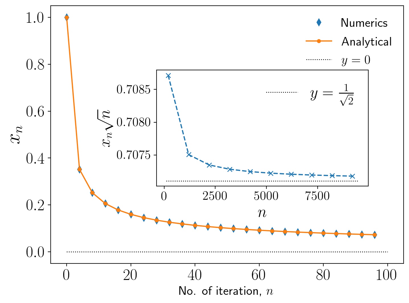
Figure 14: XXX case: (Main) Convergence to the respective fixed point $x^{*}=0$ under the map initiated with $c^{(0)}=\pi/8$, or equivalently $x_{0}=1$. (Inset) Power law behaviour for the same initial condition as seen from the convergence $x_{n}\sqrt{n}\rightarrow\frac{1}{\sqrt{2}}$ for large $n$.

C.1.2 swap-cnot-dcnot face

In this case the substitution $c_{1}^{(n)}=\pi/4$ and assuming $0\leq c_{3}^{(n)}\leq c_{2}^{(n)}\leq c_{1}^{(n)}\leq\pi/4$, simplifies the complex number arguments in the 3-dimensional map Eq. (39) to

$$\begin{split}\theta_{+}^{(n)}=&-\arctan\left[\tan c_{2}^{(n)}\tan c_{3}^{(n)}\right],\\ \theta_{-}^{(n)}=&-\arctan\left[\frac{\tan c_{3}^{(n)}}{\tan c_{2}^{(n)}}\right],\\ \phi_{+}^{(n)}=&-\arctan\left[\frac{1}{\tan c_{2}^{(n)}\,\tan c_{3}^{(n)}}\right],\\ \phi_{-}^{(n)}=&\pi-\arctan\left[\frac{\tan c_{2}^{(n)}}{\tan c_{3}^{(n)}}\right].\end{split}$$ (126)

Using above set of equations in Eq. (39) the map on Cartan coefficients reduces to

$$\begin{split}&c_{1}^{(n+1)}=\frac{\pi}{4},\\ &c_{2}^{(n+1)}=\frac{\pi}{4}\pm\frac{1}{2}\arctan\left[\sin 2\,c_{3}^{(n)}\cot 2\,c_{2}^{(n)}\right],\\ &c_{3}^{(n+1)}=\frac{1}{2}\arctan\left[\frac{\tan 2\,c_{3}^{(n)}}{\sin 2c_{2}^{(n)}}\right].\end{split}$$ (127)

Thus the map is 2-dimensional and in terms of $y_{n}=1/\tan^{2}2\,c_{2}^{(n)}$ and $z_{n}=1/\tan^{2}2\,c_{3}^{(n)}$ the above 2-dimensional map takes a purely algebraic form given by Eq. (48 ) in the main text.

C.1.3 swap-cnot edge

In this case the map on Cartan parameters is 1-dimensional; $c_{1}^{(n+1)}=\pi/4,c_{2}^{(n+1)}=c_{3}^{(n+1)}=c^{(n+1)}$, given by

$$c^{(n+1)}=\frac{1}{2}\arctan\left[\frac{1}{\cos 2\,c^{(n)}}\right].$$ (128)

In terms of $t_{n}=\tan^{2}(2\,c^{(n)})$, the above map takes a simple linear form

$$t_{n+1}=1+t_{n},$$ (129)

hence $t_{n}=n-1+t_{0}$. In terms of $y_{n}=1/\tan^{2}(2\,c^{(n)})$ reduces to Eq. (56) with exact solution given by Eq. (57). In this case the approach to the fixed point $y^{*}=0$ or, equivalently the approach of $U_{n}$ to the swap gate, is algebraic with exponent equal to 1/2 as shown in Fig. (15).

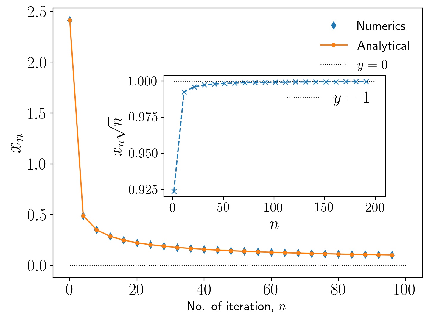
Figure 15: swap-cnot edge: (Main) Convergence to the respective fixed point $y^{*}=0$ under the map initiated with $c^{(0)}=\frac{\pi}{16}$. (Inset) Power law behaviour for the same initial condition as seen from the convergence $y_{n}\sqrt{n}\rightarrow 1$ for large $n$.

Appendix D 2-unitaries with entangled rows and columns

We write unitary operator $U$ in block form as $U=\sum_{i,j=1}^{d}\ket{i}\bra{j}\otimes X_{ij}.$

1. Unitarity of $U$: $UU^{\dagger}=U^{\dagger}U=\mathbb{I}_{d^{2}}$.

   $$UU^{\dagger} =\left(\sum_{i,j=1}^{d}\ket{i}\bra{j}\otimes X_{ij}\right)\left(\sum_{k,l=1}^{d}\ket{k}\bra{l}\otimes X_{kl}\right)^{\dagger},$$

   $$=\sum_{i,k=1}^{d}\left(\ket{i}\bra{k}\otimes\sum_{j=1}^{d}X_{ij}X_{kj}^{\dagger}\right),$$

   $UU^{\dagger}=\mathbb{I}_{d^{2}}$ gives

   $$\sum_{j=1}^{d}X_{ij}X_{kj}^{\dagger}=\delta_{ik}\mathbb{I}_{d}.$$ (130)

2. Dual-unitarity of $U$: $U^{R}U^{R\,\dagger}=U^{R\,\dagger}U^{R}=\mathbb{I}_{d^{2}}$.

   $$U^{R}U^{R\,\dagger} =\left(\sum_{ij}\ket{ij}\bra{X_{ij}^{*}}\right)\left(\sum_{kl}\ket{kl}\bra{X_{kl}^{*}}\right)^{\dagger},$$

   $$=\sum_{ij}\sum_{kl}\langle X_{kl}|X_{ij}\rangle\ket{ij}\bra{kl},$$

   $U^{R}U^{R\,\dagger}=\mathbb{I}_{d^{2}}$ gives

   $$\langle X_{kl}|X_{ij}\rangle=\delta_{ik}\delta_{jl},$$ (131)

   i.e, $X_{ij}$’s form an orthonormal operator basis.

3. T-duality of $U$: $U^{\Gamma}U^{\Gamma\,\dagger}=\mathbb{I}_{d^{2}}$.

   $$U^{\Gamma}U^{\Gamma\,\dagger} =\left(\sum_{i,j=1}^{d}\ket{j}\bra{i}\otimes X_{ij}\right)\left(\sum_{k,l=1}^{d}\ket{l}\bra{k}\otimes X_{kl}\right)^{\dagger},$$

   $$=\sum_{j,l=1}^{d}\left(\ket{j}\bra{l}\otimes\sum_{i=1}^{d}X_{ij}X_{il}^{\dagger}\right),$$

   $U^{\Gamma}U^{\Gamma\,\dagger}=\mathbb{I}_{d^{2}}$ gives

   $$\sum_{i=1}^{d}X_{ij}X_{il}^{\dagger}=\delta_{jl}\mathbb{I}_{d}.$$ (132)

The above conditions are equivalent to those presented in Ref. Rather et al. (2022) and Ref. Rico (2020) in terms of single qudit reduced density matrices (marginals) of a two-qudit pure state; $X_{ij}\mapsto\ket{X_{ij}}=(X_{ij}\otimes\mathbb{I})\ket{\Phi}$, where $\ket{\Phi}$ is the generalized Bell state. It is easy to see that the marginal with respect to the first qudit is given by $X_{ij}X_{ij}^{\dagger}$. Thus conditions (1) and (2) above involve orthonormality of sums of single qudit marginals in each row and each column respectively. A $d\times d$ arrangement of $d^{2}$-dimensional vectors (two-qudit quantum states) $\ket{X_{ij}}$ which satisfy Eqs. (130)–(132) form an orthogonal quantum Latin square (OQLS). This generalizes the notion of OLS for general 2-unitary operators not necessarily permutations or those for which single qudit marginals are projectors where each $\ket{X_{ij}}$ is a product state. The original definitions of OQLS Goyeneche et al. (2018); Musto and Vicary (2019) are fragile in the sense they do not work when $\ket{X_{ij}}$ are entangled. Note that the entanglement of two-qudit states $\ket{X_{ij}}$’s change when unitary $U=\sum_{i,j=1}^{d}\ket{i}\bra{j}\otimes X_{ij}$, is multiplied by local unitary transformations.

Appendix E Fixed point of $\mathcal{M}_{R}^{2}$ map that is not dual-unitary

Here we give an example of a fixed point of the $\mathcal{M}_{R}^{2}$ map in $d^{2}=9$ which is not dual-unitary. The unitary is given by

$$U_{\text{nd}}=\begin{pmatrix}1&0&0&0&0&0&0&0&0\\ 0&0&\sqrt{3}/2&1/2&0&0&0&0&0\\ 0&0&0&0&0&\sqrt{3}/2&-1/2&0&0\\ 0&0&0&0&0&0&0&1&0\\ 0&1&0&0&0&0&0&0&0\\ 0&0&0&0&1&0&0&0&0\\ 0&0&0&0&0&0&0&0&1\\ 0&0&-1/2&\sqrt{3}/2&0&0&0&0&0\\ 0&0&0&0&0&1/2&\sqrt{3}/2&0&0\end{pmatrix}.$$ (133)

Action of $\mathcal{M}_{R}$ map on $U_{\text{nd}}$ results in

$$U_{\text{nd}}^{\prime} :=\mathcal{M}_{R}[U_{\text{nd}}]$$ (134)

$$=\begin{pmatrix}\sqrt{3}/2&0&0&0&0&1/2&0&0&0\\ 0&0&0&0&0&0&0&0&1\\ 0&0&1/2&0&0&0&-\sqrt{3}/2&0&0\\ 0&0&0&0&1&0&0&0&0\\ 0&0&0&0&0&0&0&1&0\\ 0&1&0&0&0&0&0&0&0\\ 1/2&0&0&0&0&-\sqrt{3}/2&0&0&0\\ 0&0&0&1&0&0&0&0&-0\\ 0&0&\sqrt{3}/2&0&0&0&1/2&0&0\end{pmatrix},$$ (135)

such that $\mathcal{M}_{R}[U_{\text{nd}}^{\prime}]=U_{\text{nd}}$ i.e. $U_{\text{nd}}$ (subscript ’nd’ is used to emphasize it is not dual-unitary) is a fixed point of the $\mathcal{M}_{R}^{2}$ map

$$\mathcal{M}_{R}^{2}[U_{\text{nd}}]:=\mathcal{M}_{R}[\mathcal{M}_{R}[U_{\text{nd}}]]=\mathcal{M}_{R}[U_{\text{nd}}^{\prime}]=U_{\text{nd}}.$$

Interestingly, $U_{\text{nd}}$ and $U_{\text{nd}}^{\prime}$ are LU equivalent,

$$U_{\text{nd}}=(u_{1}\otimes u_{2})U_{\text{nd}}^{\prime}(v_{1}\otimes v_{2}),$$ (136)

where $u_{1}=\begin{pmatrix}-\sqrt{3}/2&0&-1/2\\ 0&1&0\\ -1/2&0&\sqrt{3}/2\end{pmatrix},\,u_{2}=v_{1}=\begin{pmatrix}1&0&0\\ 0&0&1\\ 0&-1&0\end{pmatrix}$, and $v_{2}=\begin{pmatrix}-1&0&0\\ 0&1&0\\ 0&0&-1\end{pmatrix}$.

$U_{\text{nd}}$ ($U_{\text{nd}}^{\prime}$) is not dual-unitary; $U_{\text{nd}}^{R}U_{\text{nd}}^{R\,\dagger}\neq\mathbb{I}$, having three distinct Schmidt values given by $\left\{1+\frac{\sqrt{3}}{2}\,,\,1\,,\,1-\frac{\sqrt{3}}{2}\right\},$ with each value repeated three times. As a consequence of LU equivalence $U_{\text{nd}}$ and $U_{\text{nd}}^{\prime}$ have the same entangling power and gate-typicality.