End-to-End Multi-Object Detection with a Regularized Mixture Model

Abstract

Recent end-to-end multi-object detectors simplify the inference pipeline by removing hand-crafted processes such as non-maximum suppression (NMS). However, during training, they still heavily rely on heuristics and hand-crafted processes which deteriorate the reliability of the predicted confidence score. In this paper, we propose a novel framework to train an end-to-end multi-object detector consisting of only two terms: negative log-likelihood (NLL) and a regularization term. In doing so, the multi-object detection problem is treated as density estimation of the ground truth bounding boxes utilizing a regularized mixture density model. The proposed end-to-end multi-object Detection with a Regularized Mixture Model (D-RMM) is trained by minimizing the NLL with the proposed regularization term, maximum component maximization (MCM) loss, preventing duplicate predictions. Our method reduces the heuristics of the training process and improves the reliability of the predicted confidence score. Moreover, our D-RMM outperforms the previous end-to-end detectors on MS COCO dataset. Code will be available.

1 Introduction

“How can we train a detector to learn a variable number of ground truth bounding boxes for an input image without duplicate predictions?” This is a fundamental question in the training of end-to-end multi-object detectors (carion2020detr). In multi-object detection, each training image has a different number of bounding box coordinates and the corresponding class labels. Thus, the network output is challenging to match one-to-one with the ground truth. Conventional methods (ren2015fasterRCNN; liu2016ssd; redmon2016yolo) train the detector by assigning a ground truth to many duplicate predictions, but they cannot directly obtain the final predictions without relying on non-maximum suppression (NMS) in the inference phase.

As an answer to the opening question, recent end-to-end multi-object detection methods address the training of detector by searching for unique assignments between the predictions and the ground truth via bipartite matching (Figure 1). The assigned positive prediction by bipartite matching learns the corresponding ground truth by a pre-designed objective function. On the other hand, the unassigned negative predictions do not care about ground truth information but are trained as backgrounds. Unlike conventional detectors, end-to-end methods can obtain final predictions from detector networks through bipartite matching-based training without relying on NMS in the inference phase.

However, the training of the current end-to-end multi-object detectors has several drawbacks as follows:
Immoderate heuristics.  In the training process, the current end-to-end methods use heuristically designed objective functions and matching criteria between the ground truth and a prediction. For instance, DETR, the representative end-to-end method, uses the following combination of losses as the training objective and matching criterion:

$$\begin{split}\mathcal{L}&=w_{1}\cdot\mathcal{L}_{CE}+w_{2}\cdot\mathcal{L}_{L1}+w_{3}\cdot\mathcal{L}_{GIoU},\end{split}$$ (1)

where, $\mathcal{L}_{CE}$, $\mathcal{L}_{L1}$, and $\mathcal{L}_{GIoU}$ are cross-entropy, L1 and GIoU (rezatofighi2019generalized) loss with its balancing hyper-parameters ($w_{1}$, $w_{2}$, and $w_{3}$) respectively. Deformable DETR (zhu2020deformable) and Sparse R-CNN (sun2021sparse), other popular end-to-end methods, replace the cross-entropy loss with the focal loss (lin2017focal).

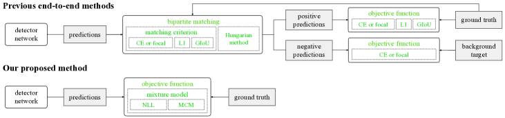
Figure 1: Training pipeline of end-to-end multi-object detectors. First row : previous end-to-end method such as (carion2020detr; sun2021sparse). Second row: our proposed method. The green text denotes the manually designed training components.

Hand-crafted assignment.  Since there are many possible pairs between ground truths and predictions, the end-to-end methods need to find an optimal set of pairs among them. To solve this assignment problem, most end-to-end detectors utilize hand-crafted algorithm such as the Hungarian method (kuhn1955hungarian) in the training pipeline to find a good bipartite matching.
Unreliable confidence.  In the aspect of the nature of human recognition, the confidence score of the prediction is regarded as an estimate of the accuracy (guo2017oncalibration). For the confidence score to be reliable, which means that the confidence score is to be used directly as an accuracy estimate, it should have a probabilistic meaning. However, in the training process based on bipartite matching, the predictions are discretely classified as either positive or negative by a hand-crafted assignment process and a heuristic matching criterion rather than from a probabilistic point of view. In addition, the weight in the focal loss, which is a general loss term to learn class probability, is controlled by hyper-parameters and does not provide a clear probabilistic basis. These heuristics and hand-designed training processes lead to gaps between predicted confidence scores and actual accuracy. Figure 2 shows the difference between the confidence score and the actual accuracy in the prediction of previous end-to-end detectors (DETR, Deformable DETR, Sparse R-CNN) and our probabilistic model (D-RMM).

In this study, we aim to overcome the aforementioned limitations and answer the opening question better. To this end, we propose a novel end-to-end multi-object detection framework, D-RMM, where we reformulate the end-to-end multi-object detection problem as a parametric density estimation problem. Our detector estimates the distribution of bounding boxes and object class using a mixture model. The proposed training loss function consists of the following two terms: the negative log-likelihood (NLL) and the maximum component maximization (MCM) loss. The NLL loss is a simple density estimation term of a mixture model. The MCM loss is the regularization term of the mixture model to achieve non-duplicate predictions. The NLL loss is calculated without any matching process, and the MCM loss only uses a simple maximum operation as matching. The contributions of our study are summarized as follows:

• We approach the end-to-end multi-object detection as a mixture model-based density estimation. To this end, we introduce an intuitive training objective function and the corresponding network architecture.

• We replace the heuristic objective function consisting of several losses with a simple negative log-likelihood (NLL) and the regularization (MCM) terms of a mixture model from a probabilistic point of view.

• Thanks to the simplicity of the NLL and MCM loss, they are directly calculated from the network outputs without any additional process, such as bipartite matching.

• As can be seen in Figure 2, the predictions of our method provide more reliable confidence scores.

• Our work outperforms the structural baselines (Sparse R-CNN, AdaMixer) and other state-of-the-art end-to-end multi-object detectors on MS COCO dataset.

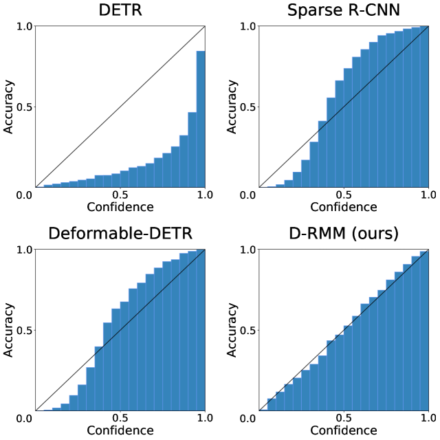
Figure 2: Confidence score vs. accuracy of various end-to-end detectors. Accuracy is measured for the predicted bounding boxes with the confidence score in the corresponding confidence bin.

2 Related Works

Most modern deep-learning-based object detectors require post-processing to remove redundant predictions (e.g. NMS) from dense candidates in estimating final bounding boxes (redmon2016yolo; liu2016ssd; ren2015fasterRCNN). Instead of depending on manually-designed post-processing, a line of recent works (hu2018relation; carion2020detr; sun2021sparse) has proposed end-to-end object detection methods which output final bounding boxes directly without any post-processing in both the training and inference phase.

Recently, end-to-end methods (hu2018relation; carion2020detr; zhu2020deformable) that do not use NMS-based post-processing have been proposed. DETR (carion2020detr) proposes the training process for end-to-end detectors using the Hungarian algorithm (kuhn1955hungarian), which yields an optimal bipartite matching between $N\times K$ samples. This training process has become a standard for end-to-end detectors. Among them, Sparse R-CNN (sun2021sparse) is one of the representative methods in which a fixed set of learned proposal boxes and features are used. Sparse R-CNN argues that it has a simpler framework than other end-to-end detectors (carion2020detr; zhu2020deformable), but it still uses Hungarian-algorithm-based bipartite matching for training.

However, the training of end-to-end detectors based on bipartite matching relies on heuristic objective functions, matching criteria, and hand-assigned algorithms. It is also known that the efficiency and stability of training are impaired due to the limited supervision by bipartite matching. (jia2022detrs; li2022dn)

Another line of research has focused on removing the heuristics of the ground truth assignment process. Among them, Mixture Density Object Detector (MDOD) (Yoo_2021_ICCV) reformulated the multi-object detection task as a density estimation problem of bounding box distributions with a mixture model. This enabled MDOD to perform regression without an explicit matching process with ground truths. However, MDOD still requires the matching process for training a classification task. Furthermore, it is not an end-to-end method and cannot replace the training process based on bipartite matching.

In this paper, we extend the density-estimation-based multi-object detector to an end-to-end method that does not need the deduplication process for the predictions. In addition, our D-RMM is trained as an end-to-end detector by directly calculating the loss from the network outputs, unlike other end-to-end methods that rely on an additional process such as the Hungarian method for bipartite matching. Our work greatly simplifies the training process of the end-to-end multi-object detector by using a straightforward strategy.

3 The D-RMM Framework

3.1 Mixture model

For the multiple ground truths $g=\{g_{1},...,g_{N}\}$ on an image $X$, each ground truth $g_{i}$ contains the coordinates of an object’s location $b_{i}=\{b_{i,l},b_{i,t},b_{i,r},b_{i,b}\}$ (left, top, right, and bottom) and a one-hot class information $c_{i}$. The D-RMM network conditionally estimates the distribution of the $g$ for an image $X$ using a mixture model.

The mixture model consists of two types of probability distribution: Cauchy (continuous) for bounding box coordinates and categorical (discrete) for class estimation. The Cauchy distribution is a continuous probability distribution that has a shape similar to the Gaussian distribution. However, it has heavier tails than the Gaussian, and is known to be less likely to incur underflow problems due to floating-point precision (Yoo_2021_ICCV). We use the 4-dimensional Cauchy to represent the distribution of the object’s location coordinates. Also, a categorical distribution is used to estimate the object’s class probabilities for the one-hot class representation. The probability density function of our mixture model is defined as follows:

$$p(g_{i}|X) =\sum_{k}^{K}\pi_{k}\mathcal{F}(b_{i};\mu_{k},\gamma_{k})\mathcal{P}(c_{i};p_{k}).$$ (2)

Here, the $k$ is the index for the $K$ mixture components and the corresponding mixing coefficient is denoted by $\pi_{k}$. $\mathcal{F}$ and $\mathcal{P}$ denote the probability density function of the Cauchy and the probability mass function of the categorical distribution  respectively. The parameters $\mu_{k}=\{\mu_{k,l},\mu_{k,t},\mu_{k,r},\mu_{k,b}\}$ and $\gamma_{k}=\{\gamma_{k,l},\gamma_{k,t},\gamma_{k,r},\gamma_{k,b}\}$ are the location and scale parameters of a Cauchy distribution, while $p_{k}=\{p_{1},...,p_{C}\}$ is the class probability of a categorical distribution. Here, $C$ is the number of possible classes for an object excluding the background class. To avoid over-complicating the mixture model, each element of $b_{i}$ is assumed to be independent of others. Thus, the probability density function of the Cauchy is factorized as

$$\mathcal{F}(b_{i};\mu_{k},\gamma_{k}) =\prod_{j\in D}\mathcal{F}(b_{i,j};\mu_{k,j},\gamma_{k,j}),\quad D=\{l,t,r,b\}.$$ (3)

3.2 Architecture

For the implementation of our D-RMM, we adopt the overall architecture of Sparse R-CNN (sun2021sparse) and its network characteristics such as learnable proposal box, dynamic head, and iteration structure due to the intuitive structure and fast training compared to the DETR (carion2020detr) and Deformable DETR (zhu2020deformable). Also, we applied D-RMM to AdaMixer (gao2022adamixer) while maintaining its structural characteristics.

Figure 3 shows the overview of our D-RMM network when the 3-stage iteration structure is used. First, the backbone network outputs the feature map from the input image $X$. In the first stage, a set of RoI features $h^{1}=\{h_{1}^{1},...,h_{K}^{1}\}$ is obtained through RoI align process from the predefined learnable proposal boxes $\bar{b}^{1}=\{\bar{b}_{1}^{1},...,\bar{b}_{K}^{1}\}$ and the feature map. Then, D-RMM head predicts $M^{1}=\{\pi^{1},\mu^{1},\gamma^{1},p^{1},o^{1}\}$, the parameters of the mixture model ($\pi^{1},\mu^{1},\gamma^{1},p^{1}$) and the objectness score ($o^{1}$), from $h^{1}$. Here, the number of mixture components $K$ equals the number of proposal boxes. In the $s$-th stage ($s\geq 2$), the process from RoI align to D-RMM head is repeated. $\mu^{s-1}\in\mathbb{R}^{4}$ which is the predicted location vector in the previous stage, is used as the proposal boxes $\bar{b}^{s}$ for the current stage $s$. Following (sun2021sparse), we adopt the 6-stage iteration structure.

The details of D-RMM head are illustrated in Figure 4. The dynamic head outputs $\bar{\mu}_{k}^{s},\bar{\gamma}_{k}^{s},\bar{p}_{k}^{s}$ and $\bar{o}_{k}^{s}$ from $h_{k}^{s}$. The location parameter $\mu_{k}^{s}\in\mathbb{R}^{4}$ represents the coordinates of a mixture component and is produced by adding $\bar{b}_{k}^{s}$ to $\bar{\mu}_{k}^{s}$. The positive scale parameter $\gamma_{k}^{s}\in\mathbb{R}^{4}$ is obtained by applying the softplus activation (dugas2000softplus) that always converts $\bar{\gamma}_{k}^{s}$ into a positive value. The object class probability $p_{k}^{s}\in\mathbb{R}^{C}$ is calculated by applying softmax function to $\bar{p}_{k}^{s}$ along the class dimension.

Note that, the probability of whether it is an object or not is not computed through $p_{k}^{s}$ but computed using an alternative way we propose to learn objectness score. Returning to the nature of the probability distribution, we utilize the properties of the mixture model. In the mixture model, the probability of a mixture component is expressed as a mixture coefficient $\pi_{k}^{s}$. In other words, the mixture component that is likely to belong to an object area has a higher $\pi_{k}^{s}$ value. In this aspect, we assume that $\pi$ could be regarded as the scaled objectness score such that $\sum_{k}^{K}\pi_{k}^{s}$ equals 1. From this assumption, we propose to express the mixture coefficient $\pi$ using the objectness score $o$. As shown in Figure 4, the sigmoid activation outputs $o_{k}^{s}$ from $\bar{o}_{k}^{s}$. And then, $\pi_{k}^{s}$ is calculated by normalizing $o_{k}^{s}$ as $\pi_{k}^{s}=\frac{o_{k}^{s}}{\sum_{k^{\prime}=1}^{K}o_{k^{\prime}}^{s}}$.

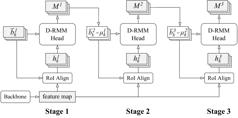
Figure 3: 3-stage example of D-RMM architecture. D-RMM head predicts the mixture model’s parameters $M^{s}$ from the proposal boxes $\bar{b}_{k}^{s}$ and an input image $X$.

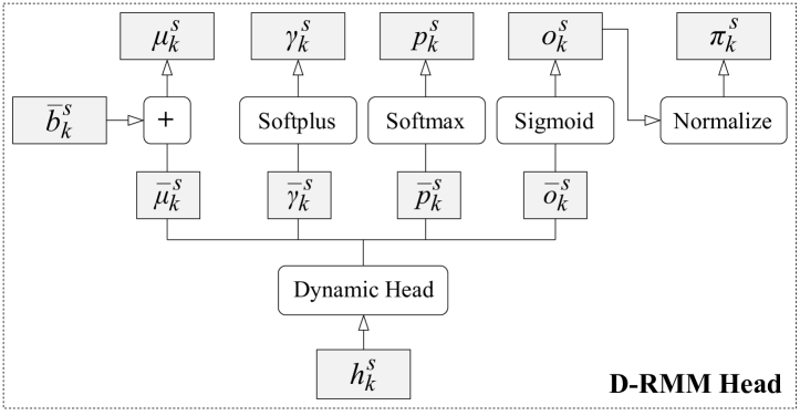
Figure 4: Structure of D-RMM head. D-RMM head predicts the parameters of the mixture model ($\pi_{k}^{s}$, $\mu_{k}^{s}$ $\gamma_{k}^{s}$ and $p_{k}^{s}$) and the objectness score ($o_{k}^{s}$) from a proposal box $\bar{b}_{k}^{s}$ and a RoI feature $h_{k}^{s}$.

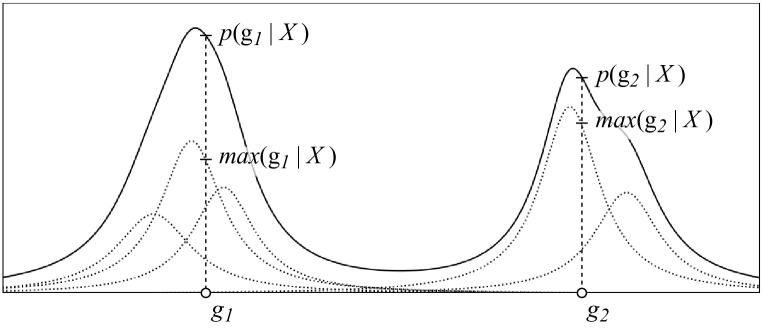
Figure 5: Illustration of 1-D example for the MCM loss ($\mathcal{L}_{MCM}$). By reducing the difference between $max(g_{i}|X)$ and $p(g_{i}|X)$, it is trained to require only one mixture component to represent one $g_{i}$. Hence it restrains from having multiple components to represent the same single $g_{i}$.

3.3 Training

The D-RMM network is trained to maximize the likelihood of $g$ for the input image $X$ through the mixture model. The loss function is simply defined as the negative log-likelihood (NLL) of the probability density function as follows:

$$\mathcal{L}_{NLL} =-\log p(g_{i}|X)$$ (4)

$$=-\log\sum_{k}^{K}\pi_{k}^{s}\mathcal{F}(b_{i};\mu_{k}^{s},\gamma_{k}^{s})\mathcal{P}(c_{i};p_{k}^{s})$$ (5)

The D-RMM network learns the coordinates of the bounding box and the probability of the object class as $\mu$ and $p$ by minimizing the NLL loss ($\mathcal{L}_{NLL}$). The mixture coefficient $\pi$ learns the probability of a mixture component $\mathcal{F}(b_{i})\mathcal{P}(c_{i})$ that represents the joint probability for both box coordinates and object class. The objectness score $o$ is not directly used to calculate the NLL loss, but it is trained through $\pi$ (see Figure 4).

Here, we need to consider that the NLL loss does not restrict the distributional redundancy between multiple mixture components for single ground truth. This problem could lead to duplication of the predicted bounding boxes, as well as dispersion of the probability for one object to several mixture components. Thus, we introduce the maximum component maximization (MCM) loss which is the regularization term to the density estimation of the mixture model:

$$\mathcal{L}_{MCM} =-\log\frac{\max(g_{i}|X)}{p(g_{i}|X)}$$ (6)

$$=-\log\frac{\max(g_{i}|X)}{\sum_{k=1}^{K}\pi_{k}^{s}\mathcal{F}(b_{i};\mu_{k}^{s},\gamma_{k}^{s})\mathcal{P}(c_{i};p_{k}^{s})},$$ (7)

$$\max(g_{i}|X) =\max_{k\in\{1,...,K\}}(\pi_{k}^{s}\mathcal{F}(b_{i};\mu_{k}^{s},\gamma_{k}^{s})\mathcal{P}(c_{i};p_{k}^{s}))$$ (8)

Figure 5 shows 1-D example for the MCM loss ($\mathcal{L}_{MCM}$). Minimizing the MCM loss reduces the difference of likelihood between $max(g_{i}|X)$ and $p(g_{i}|X)$. Through this, the mixture model is trained to maximize the probability of only one mixture component for one ground truth while reducing the probability of other adjacent components. The total loss function is defined as follows: $\mathcal{L}=\mathcal{L}_{NLL}+\beta\times\mathcal{L}_{MCM}$, where $\beta$ balances between the NLL and the MCM loss. The total loss ($\mathcal{L}$) is computed for all stages of D-RMM, then summed together and back-propagated. To calculate the total loss, we do not need any additional process such as bipartite matching.

3.4 Inference

In the inference, $\mu$ of the last stage is used as the coordinates of the predicted bounding boxes. The class probability $p_{k}\in\mathbb{R}^{C}$ of $k$-th mixture component is the softmax output but, just the probability for the class of an object without background probability. Thus, we do not directly use $p$ as a confidence score of our prediction. Instead, the objectness score $o$ learned though the mixing coefficient $\pi$ is used with $p$. The confidence score of an $k$-th output prediction for class $c$ is calculated as $p_{k,c}\times o_{k}$ where $p_{k,c}$ is the $c$-th element of $p_{k}$. In the same manner as other end-to-end multi-object detectors, D-RMM also obtains final predictions without any duplicate bounding box removal process such as NMS.

4 Experiments

4.1 Experimental details

Dataset.  We evaluate D-RMM on MS COCO 2017 (lin2014microsoft). Following the common practice, we split the dataset into 118K images for the training set, 5K for the validation set, and 20K for the test-dev set. We adopt the standard COCO AP (Average Precision) and AR (Average Recall) at most 100 top-scoring detections per image as the evaluation metrics. We report analysis results and comparison with a baseline on the validation set and compare with other methods on the test-dev and validation set.

Training.  As mentioned in Section 1 and 3.1, we model bounding box coordinates as Cauchy distributions and class probability as categorical distributions. We applied D-RMM to Sparse R-CNN (S-RCNN) and AdaMixer. For analysis, we adopt Sparse R-CNN architecture with 300 proposals. Unless specified, we followed the hyper-parameters of each original paper. As backbones, ResNet50 (R50), ResNet101 (R101) (he2016resnet) and Swin Transformer-Tiny (Swin-T) (liu2021swin) with Feature Pyramid Network (FPN) (lin2017feature) are adopted, which are pretrained on ImageNet-1K (imagenet). The parameter $\beta$ for balancing the losses $\mathcal{L}_{NLL}$ and $\mathcal{L}_{MCM}$ is set to 0.5. $\beta$ was found experimentally, and related experiments are in Appendix Section LABEL:appendix:sec:mcm_beta. Synchronized batch normalization (peng2018megdet) is applied for consistent learning behavior regardless of the number of GPUs. More details like batch size, data augmentation, optimizer and training schedule for reproducibility are in Appendix LABEL:appendix:sec:training_details.

Inference.  We select top-100 bounding boxes among the last head output according to their confidence scores without any further post-processing, such as NMS.

4.2 Comparison with Sparse R-CNN

Table 1 presents a comparison between Sparse R-CNN and D-RMM with different backbone networks on COCO validation set. We achieve significant AP improvement over Sparse R-CNN while maintaining the FPS on a similar level. There exists a slight gain ($\leq$ 0.1 FPS) in inference speed due to implementation details. The analysis of performance improvement is as follows.

Table 1: Comparison with Sparse R-CNN (sun2021sparse). FPS is measured as a network inference time excluding data loading on a single NVIDIA TITAN RTX using MMDet (mmdetection) with batch size 1.

Method	Backbone	AP	AP50	AP75	FPS
S-RCNN	R50 FPN	45.0	64.1	49.0	22.7
D-RMM		47.0	64.8	51.6	22.8
S-RCNN	R101 FPN	46.4	65.6	50.7	17.3
D-RMM		48.0	65.7	52.6	17.3
S-RCNN	Swin-T FPN	47.4	67.1	52.0	16.4
D-RMM		49.9	68.1	55.1	16.5

Table 2: $B$ denotes Bipartite Matching, $M$ denotes Max. Both the matching cost and objective function of the 2nd row are the NLL loss. And in the case of the objective function, the NLL loss is computed only for matched predictions. In other words, unlike the 3rd-5th rows, the 2nd row is not a mixture model.

Method	REG	CLS	NLL	MCM	AP
S-RCNN	$\checkmark(B)$	$\checkmark(B)$			45.0
			$\checkmark(B)$		46.3
			$\checkmark$		35.6
			$\checkmark$	$\checkmark(B)$	46.9
D-RMM			$\checkmark$	$\checkmark(M)$	47.0

Objective function.  In Table 2, we compared the APs by varying the objective function and observed the following. First, in Sparse R-CNN, modeling the objective function and the matching cost jointly with the NLL loss is more effective in performance than a combination of semantically different regression and classification losses (45.0$\rightarrow$46.3). Second, the performance of the NLL loss with a mixture model is relatively low because there is no means to remove duplicate bounding boxes (35.6). Third, the MCM loss to remove duplicates significantly improves the AP (35.6$\rightarrow$46.9). Fourth, the AP is slightly increased even if the matching method for the MCM loss is changed to a simple MAX function (46.9$\rightarrow$47.0). Also, D-RMM significantly outperforms Sparse R-CNN.

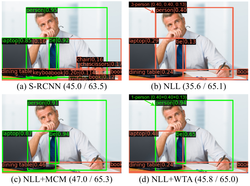
Figure 6: Qualitative result. Red/Green boxes indicate confidence 0.1-0.5 and 0.5-1.0, respectively. ‘/’ separates AP/AR

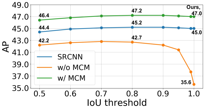
Figure 7: NMS result. The IoU threshold=1.0 means that NMS is not performed.

Visualization.  Figure 6 (a), (b), (c) visualize the 1st, 3rd, and last rows of Table 2. As shown in (a) and (c), the inference results with confidence scores of 0.5 or higher are quite similar. However, with the confidence scores below 0.5, S-RCNN results are rather noisy. Although (b) seems to show comparable results to (c), the confidence scores of (b) tend to be lower than those of (c), and many overlapping boxes exist. For example, in (b), there are 3-overlapping boxes with low confidence scores of {0.40, 0.40, 0.13}. Within the mixture model framework, the likelihood of (b) might be similar to (c). It will be further discussed in Section LABEL:sec:lms_loss_and_deduplication. More examples are in Appendix LABEL:appendix:sec:more_visualization.

As shown in the figure, (b) has many duplicates. Interestingly, (b) and (c) has a large AP gap, but AR is similar. We conjectured the MCM loss contributed significantly to deduplication. Therefore, we conducted related experiments.

Table 3: Handicraft method for merging confidences by applying the winner-take-all strategy (WTA).