Optimal sequences for pairwise comparisons: the graph of graphs approach

Abstract

In preference modelling, it is essential to determine the number of questions and their arrangements to ask from the decision maker. We focus on incomplete pairwise comparison matrices. First, optimal incomplete filling in patterns are identified, resulting in weight vectors being closest (on average) to that of the complete case. These results are obtained by extensive numerical simulations with large sample sizes. Optimal filling in sequences, formed by optimal or near optimal filling patterns, are found in the GRAPH of representing graphs. The star graph is revealed to be optimal among spanning trees, while the optimal graphs are always close to bipartite ones. Regular graphs appear to also correspond to optimal cases, furthermore regularity holds all optimal graphs, as the degrees of different vertices are always as close to each other as possible. The practical relevance of the results includes the cases when the decision maker can abandon the problem at any period of the process, e.g., in online questionnaires. However, the found patterns are potentially applicable in a wide range of models of preference and information theory.

Keywords: pairwise comparison, incomplete pairwise comparison matrix, graph of comparisons, filling in sequence, GRAPH of graphs;

1 Introduction

The concept of pairwise comparisons (Thurstone,, 1927) is fundamental in preference modelling, ranking and Multicriteria Decision Making (MCDM) (Triantaphyllou,, 2000). These comparisons are frequently given in the form of pairwise comparison matrices (PCMs), which are the basis of the Analytic Hierarchy Process (AHP) (Bernasconi et al.,, 2010; Saaty,, 1977, 1980; Wind and Saaty,, 1980). Incompleteness (the absence of some comparisons) occurs quite often in practical problems (Bozóki et al.,, 2016), as well as in theoretical questions (Fedrizzi and Giove,, 2007; Bozóki et al.,, 2010; Csató and Rónyai,, 2016; Kułakowski and Talaga,, 2020). In connection with decision making problems, one major source of missing data is the lack of willingness or time of the decision maker, as completing all comparisons – especially in case of many different levels, criteria and alternatives – can be exhausting and lingering (Szádoczki et al., 2022b, ; Fedrizzi and Giove,, 2013).

The arrangement of comparisons, which has a crucial effect on the results, is often represented by graphs (Gass,, 1998), where the vertices denote the alternatives and the edges stand for comparisons. In this paper we provide the optimal filling in patterns of incomplete pairwise comparison matrices, which on average produce the (both cardinally and ordinally) closest weight vectors to the complete case, for at most six alternatives (criteria) ($n$) for all possible given number of comparisons ($e$), when the respective graph is connected. These optimal patterns for the examined $(n,e)$ pairs are significant findings alone, however they result in (partial) optimal filling in sequences, which can be instrumental in case of such problems (e.g., online questionnaires), where the decision makers can abandon the problem at any period of the process. Furthermore, the found structures are potentially applicable with similar properties (a sense of optimality) in a wide range of models of preference and information theory.

Formal definitions on pairwise comparison matrices and their graph representation can be found in Appendix  A.

In the analysis of filling in sequences, the focus of the paper, but also in structural analysis of graphs and graph sequences in general, GRAPH of graphs is a convenient and efficient tool for research and visualization, too. NODEs of a GRAPH are graphs, and there is an EDGE between two NODEs (=graphs) if the associated graphs are in a specified relation, e.g., they can be drawn from each other by adding or deleting an edge. Depending on the specification of the relation, several GRAPHs of graphs have been investigated, see for instance Lovász, (1977). Another remarkable GRAPH of graphs is the Petersen family of seven graphs, including the Petersen graph itself (Hashimoto and Nikkuni,, 2013). The GRAPH of graphs by Mesbahi, (2002) is motivated by the evolution of graphs in a dynamic system.

It is worth noting that the term ‘neighbouring graphs’ in Lovász, (1977) is used synonymously for ‘there is an EDGE between two graphs’. Analogously, ‘reachable’ in Mesbahi, (2002) means that there is a PATH between two graphs. We use the concept of GRAPH of graphs to visualize our findings throughout the paper.

The rest of the paper is organized as follows. The methodology of the applied simulations are detailed in Section 2, while Section 3 contains the results, the optimal filling in sequences for the examined cases. Finally, Section 4 concludes and raises research questions for the future.

2 Methodology

Our aim is to find the filling structures of incomplete PCMs that provide the closest results to the complete case for a given $(n,e)$ pair, number of alternatives (criteria) and comparisons. As it is assumed that we do not have any prior information, and so, the different items are not distinguished, we used Wolfram Mathematica (Wolfram Research,, 2021), nauty and Traces (McKay and Piperno,, 2014), and IGraph/M (Horvát,, 2020) to generate every non-isomorphic (representing) graph for the examined $(n,e)$ pairs. Our extensive numerical simulations are based on the filling patterns related to these graphs. The used simulation methods are following Szádoczki et al., 2022a , however they only focus on some special cases based on smaller samples, while we compare all the possible incomplete filling structures.

The simulation’s methodology is detailed in Appendix B, and summarized below.

In order to measure the differences between the weight (prioritization) vectors, we apply commonly used cardinal and ordinal indicators, the Euclidean distance ($d_{euc}$) and the Kendall rank correlation coefficient (Kendall’s $\tau$).

We always compare the weight vector calculated from a given filling structure to the one computed from the complete PCM. Because of that, a higher value of Kendall’s $\tau$ indicates a better performance of the given filling pattern. However, the Euclidean distance can be interpreted as an error, thus its smaller level is preferred. It is also worth mentioning that besides these, Szádoczki et al., 2022a used many different kinds of measures for the special cases examined by them, and all of those provided similar results.

An instrumental part of our methodology is to determine the sample size needed in the simulations, which is based on a certain form of Chebyshev’s inequality (Steliga and Szynal,, 2010; Saw et al.,, 1984) that leads to the weak law of large numbers.

Based on that we used a sample size of 1 000 000 cases that results in given margin of errors and significance levels to determine the significant differences between the filling patterns.

The results of the eigenvector (EV) weight calculation technique is similar to the logarithmic least squares method (LLSM), but its computational time is larger. This pattern is even stronger in the case of incompleteness (for incomplete EV (CREV) and incomplete LLSM, see for instance Csató, (2013)), thus due to the large sample sizes, in our simulations we mainly focus on the LLSM weight calculation technique. The results of the CREV method were computed for smaller cases ($n\leq 5$) with a sample size of 500 000 as well, however, the ranking of filling patterns were always the same, and the indicators were almost always closer to the LLSM outcomes than the margin of error, thus we decided not to present them in many detail.

We applied three different levels (weak, modest and strong) of perturbation resulting in different inconsistency classes of PCMs.

3 Results

It is important to note that the interesting cases for our research start above three alternatives ($n$), as in case of $n=2$ and $n=3$ there is always one non-isomorphic (representing) graph for every relevant pair of $(n,e)$ as it is shown in Figure 1.

Figure 1: The connected non-isomorphic representing graphs for $n\leq 3$.

The $n=4$ case also contains only a few possibilities, but it can be interesting in a decision problem, when there are several criteria and four alternatives, and it helps to understand the results for larger examples as well. Figure 2 presents the connected representing graphs for $n=4$ as a GRAPH of graphs. The value of $e$ is shown in every row of the GRAPH, in which an EDGE between two NODEs (=graphs) denotes that we can obtain one graph from the other one by adding (or deleting) exactly one edge. The GRAPH of graphs in Figure 2 is a 4-partite GRAPH with a further specific property, namely, that EDGEs go between levels $k$ and $k+1$ only ($k=1,2,3$). Note that if all EDGEs would be oriented ‘downwards’ (i.e., the addition of an edge in the graph of comparisons), a partially ordered set of graphs (of comparisons) would be resulted in. We denote the graph that provided the weight vectors with the smallest average Euclidean distance and the largest average Kendall’s $\tau$ respect to the vectors calculated from the complete case by green background color for every $e$. If two optimal graphs are connected with an EDGE, then it is a partial optimal sequence, and the respective EDGE is also denoted by green. It is important to note that the relevant values for $e$ (the number of comparisons) are between $n-1$ (spanning trees) and $n(n-1)/2$ (complete graphs representing complete PCMs).

Figure 2: The GRAPH of graphs for $n=4$, the optimal graph for a given $e$ is highlighted by green, EDGEs between optimal graphs are colored green.

Among the spanning trees the star graph provided the smallest errors (Euclidean distances) and the largest Kendall’s $\tau$ measures. This is not connected to the optimal graph with four edges, which is the $2$-regular cycle. However, from this point on the optimal graphs result in an optimal filling sequence. This is not surprising, as for $e=5$ and $e=6$ there is only one possible non-isomorphic representing graph, but this example probably helps to understand the following cases. Tables 1 and 2 present the results provided by the graphs with $(n=4,e=3)$ and $(n=4,e=4)$ respectively, in case of the different perturbation levels. The name of the optimal graph, and the best values in every column are highlighted with green background color.

Graph	Weak		Modest		Strong
	$d_{euc}$	Kendall’s $\tau$	$d_{euc}$	Kendall’s $\tau$	$d_{euc}$	Kendall’s $\tau$
Star graph	0.0918	0.7306	0.1293	0.6639	0.1620	0.6164
Line graph	0.0967	0.7194	0.1361	0.6501	0.1701	0.6020

Table 1: The average Euclidean distances and Kendall’s $\boldsymbol{\tau}$ measures for the graphs with $\boldsymbol{(n=4,e=3)}$ in case of the different perturbation levels.

Graph	Weak		Modest		Strong
	$d_{euc}$	Kendall’s $\tau$	$d_{euc}$	Kendall’s $\tau$	$d_{euc}$	Kendall’s $\tau$
Not regular graph	0.0650	0.8027	0.0920	0.7496	0.1156	0.7111
$2$-regular graph	0.0543	0.8216	0.0771	0.7705	0.0970	0.7328

Table 2: The average Euclidean distances and Kendall’s $\boldsymbol{\tau}$ measures for the graphs with $\boldsymbol{(n=4,e=4)}$ in case of the different perturbation levels.

Based on the tables, one can observe that for a given $(n,e)$ pair, always the same graphs provided the best results. There are indeed significant differences between the examined graphs. It is also easy to see that a stronger perturbation results in higher errors, while an additional edge leads to smaller distances and higher ordinal correlations. Figure 3 presents the relation between the number of comparisons ($e$) and the analyzed cardinal ($d_{euc}$) and ordinal (Kendall’s $\tau$) measures, which can help practitioners to determine the minimal sufficient number of comparisons in a given problem. Note that Figure 3 shows the results for the optimal graphs for every $e$, thus one optimal value is not necessarily reachable from the previous one, only in case of partial optimal sequences.

If we know in advance that the decision maker is willing to provide exactly $e=n-1=3$ comparisons, then, according to Figure 2, we recommend the star graph, i.e., filling in one (e.g. the first) row/column of the pairwise comparison matrix, namely elements $a_{12},a_{13}$ and $a_{14}$ (in any order), also summarized in Table 3.

	1	2	3	4
1		#1’	#2’	#3’
2
3
4

Table 3: Filling in sequence for n = 4, e = 3. Orders with ’ are interchangeable.

In case we can assume that the decision maker is willing to provide more than three comparisons, the optimal filling in sequence is $\{a_{12},a_{23},a_{34},a_{14}\}$ (the first four elements can be asked in any order), followed by $a_{13}$ and finally $a_{24},$ also summarized in Table 4.

	1	2	3	4
1		#1’	#5	#4’
2			#2’	#6
3				#3’
4

Table 4: Filling in sequence for n = 4, e $>$ 3. Orders with ’ are interchangeable.

Figure 3: The relation between the number of comparisons ($e$), the errors (Euclidean distances) and Kendall’s $\tau$ measures of optimal graphs for $n=4$.

For larger number of alternatives (criteria, $n$), the possible number of connected graphs increases quickly, thus it is even more relevant to determine the optimal filling structure. In case of $n=5$, there are $21$ connected graphs altogether. Their 7-partite GRAPH of graphs can be seen in Figure 4, using the same notations as before.

Figure 4: The GRAPH of graphs for $n=5$, optimal graphs are highlighted by green.

One can see many similarities with the previous outcomes. The star graph resulted in the smallest Euclidean distance and the largest Kendall’s $\tau$ measure among the spanning trees, once again. It is not connected to the optimal graph with $e=5$, which is the $2$-regular cycle, as before. The next optimal graph with $e=6$ is not connected to the cycle, as well, however, from that point on there is a partial optimal sequence to the complete filling of the represented PCM. Somewhat surprisingly, the graphs providing the smallest Euclidean distances resulted in the largest Kendall’s $\tau$ for every single case, except for $e=8$. However, in that case the difference between the Kendall’s $\tau$ measures for the two possible graphs is within the margin of error, thus we highlighted the graph that is better according to the Euclidean distance, which is better in both indicators if we consider the CREV weight calculation technique. It is worth mentioning that this graph is the $3$-quasi-regular graph on $n=5$.

Figure 5 shows the relation between the number of comparisons ($e$) and the analyzed measures for $n=5$ in case of optimal graphs. One optimal value is not necessarily reachable from the previous one, as before. Minimal thresholds could be determined for the number of comparisons based on this figure for certain decision problems.

If we know in advance that the decision maker is willing to provide exactly $e=n-1=4$ comparisons, then, according to Figure 4, we recommend the star graph, i.e., filling in one (e.g. the first) row/column of the pairwise comparison matrix, namely elements $a_{12},a_{13},a_{14}$ and $a_{15}$, also summarized in Table 5.

	1	2	3	4	5
1		#1’	#2’	#3’	#4’
2
3
4
5

Table 5: Filling in sequence for n = 5, e = 4. Orders with ’ are interchangeable.

In case the decision maker is willing to provide exactly $e=n=5$ comparisons, then we should ask the elements along an $n$-cycle, e.g., $\{a_{12},a_{23},a_{34},a_{45}$ and $a_{15}\}$ (the five elements can be asked in any order), also summarized in Table 6.

	1	2	3	4	5
1		#1’			#5’
2			#2’
3				#3’
4					#4’
5

Table 6: Filling in sequence for n = 5, e = 5. Orders with ’ are interchangeable.

When we can assume that the decision maker is willing to provide more than five comparisons, the optimal filling in sequence is $\{a_{14},a_{15},a_{24},a_{25},a_{34},a_{35}\}$ (the first six elements can be asked in any order), followed by $a_{12},a_{13},a_{45},$ and finally $a_{23},$ also summarized in Table 7.

	1	2	3	4	5
1		#7	#8	#1’	#2’
2			#10	#3’	#4’
3				#5’	#6’
4					#9
5

Table 7: Filling in sequence for n = 5, e > 5. Orders with ’ are interchangeable.

Figure 5: The relation between the number of comparisons ($e$), the errors (Euclidean distances) and Kendall’s $\tau$ measures of optimal graphs for $n=5$.

Finally, for $n=6$, there are $112$ possible connected (representing) graphs. Figure 6 shows the 11-partite GRAPH of graphs for this case, however, in order to keep it visible, we only denote the possible graphs with a vertex, and present the optimal cases in detail in Figure 7. For $e=12$ and $e=13$ the results are close to each other, and some of the differences of the Kendall’s $\tau$ measures are also smaller, than the margin of error. Here the best graph according to the Euclidean distance and the Kendall’s $\tau$ are different as well. However, we highlighted the graphs which were at least second according to at least one indicator by a lighter green color. These highlighted graphs for a given $e$ practically provide the same results. As there is always a unique optimal graph according to the Euclidean distance, we denoted those with an $E$. We have not highlighted the EDGEs by green color on this part of the GRAPH of graphs, because of the similar results (ties). In Figure 7 for $e=12$ and $13$ the graphs that provided the best results according to the Euclidean distance are presented.

If we know in advance that the decision maker is willing to provide exactly $e=n-1=5$ comparisons, then, according to Figure 6, we recommend the star graph, i.e., filling in one (e.g. the first) row/column of the pairwise comparison matrix, namely elements $a_{12},a_{13},a_{14},a_{15}$ and $a_{16}$, also summarized in Table 8.

	1	2	3	4	5	6
1		#1’	#2’	#3’	#4’	#5’
2
3
4
5
6

Table 8: Filling in sequence for n = 6, e = 5. Orders with ’ are interchangeable.

In case we can assume that the decision maker is willing to provide more than five comparisons, the recommended filling in sequence is $\{a_{14},a_{15},a_{24},a_{26},a_{35},a_{36}\}$ (the first six elements can be asked in any order), followed by $\color[rgb]{1,.5,0}a_{25},a_{34},\color[rgb]{0,0,0}a_{16},a_{12},a_{46},\color[rgb]{1,.5,0}a_{23},a_{45},\color[rgb]{0,0,0}a_{56},$ and finally $a_{13},$ also summarized in Table 9.

	1	2	3	4	5	6
1		#10	#15	#1’	#2’	#9
2			#12	#3’	#7	#4’
3				#8	#5’	#6’
4					#13	#11
5						#14
6

Table 9: Filling in sequence for n = 6, e > 5. Orders with ’ are interchangeable.

Since there is no path along all the optimal graphs, the filling in sequence above includes as many as possible. The remaining EDGEs are colored with orange in Figure 6, and we should note that the other included graphs are as close to optimal ones as possible.

Figure 6: The GRAPH of graphs for $n=6$, optimal graphs (=NODEs) are colored green, EDGEs between optimal graphs are colored green, too.

Figure 7: The optimal graphs related to the green NODEs in Figure 6. The second row shows a partial optimal filling sequence corresponding to the one in Figure 6, these graphs can be reached from each other. The additional comparisons are highlighted in every step.

One can observe many similarities with the earlier outcomes in connection with the concrete graphs, and the pattern of optimal graphs as well. Among the spanning trees, the star graph provided the best results according to both measures again. For $e=6$ the $2$-regular cycle turned out to be the optimal case, just as earlier. The optimal graphs with $e=5,6$ and $7$ are not connected, but from that point on we can determine an optimal filling in sequence to the complete graph (if we consider all the light green cases optimal).

Moreover, for $e=9$ the optimal graph is the single bipartite $3$-regular graph on six vertices, while for $e=12$ the highlighted graph, which provided the best results according to the Euclidean distance and the second best according to the Kendall’s $\tau$, is the only $4$-regular graph on six vertices. Based on the simulations, we can make several important remarks.

Remark 1

The star graph provided the best results according to both measures for all examined $(n,e=n-1)$ cases. Thus we can say that it is an optimal structure, intuitively it keeps this property for larger cases $(n)$, as well.

Remark 2

For the $(n,e=k\cdot n)$ examples, the optimal graph is always a $k$-regular graph. Furthermore, $k$-quasi-regular graphs are optimal as well. One can say that regularity is indeed important in a more general way, as in all of the examined instances, the degree of different vertices (the number of comparisons) are as close as possible.

Remark 3

The optimal graphs are always bipartite graphs, or the closest ones to that.

The analyzed indicators for optimal graphs in the case of different number of comparisons ($e$) can be seen in Figure 8 for $n=6$. Again, it can serve as a guide for practitioners.

Figure 8: The relation between the number of comparisons ($e$), the errors (Euclidean distances) and Kendall’s $\tau$ measures of optimal graphs for $n=6$.

All of our simulation results provided optimal filling structures (representing graphs) for the examined $(n,e)$ pairs, as well as (partial) optimal filling sequences. The outcomes show indeed similar patterns for different parameters, and can support both applications and theoretical studies.

4 Conclusion and further research

In this paper we analyzed all possible filling structures of incomplete pairwise comparison matrices when there is no prior information available for the compared items, in the case of at most six alternatives (criteria). The study heavily relied on the representing graphs of pairwise comparisons as well as on extensive numerical simulations with large samples. We compared the weight vectors (calculated by the incomplete LLSM) related to the certain filling patterns and compared them based on their Euclidean distance and Kendall’s $\tau$ measure with the weights obtained from the complete case.

We found that there is a strong connection between the examined cardinal and ordinal indicators, thus we could determine the best filling structure for a given number of alternatives and comparisons. Many of these optimal graphs resulted in optimal filling in sequences as illustrated by different paths in the examined GRAPHs of graphs.

The filling structure represented by a star graph turned out to be optimal among the graphs (filling patterns) with the same cardinality (spanning trees). Regular graphs also seem to provide optimal solutions, and regularity is a common property of the optimal cases in a more general sense.

Both theorists and practitioners can utilize our findings not just to apply the optimal filling structure in their problems, but also to use the optimal filling sequences in decision making problems where the decision maker can abandon the problem at any period of the process. Furthermore, our results on the difference between the optimal patterns and the complete case for different number of comparisons can serve as a guide to determine the minimal sufficient number of comparisons for a given problem.

A future research can investigate the certain comparisons that decrease the errors the most during the filling in process. When should we stop to ask even more questions from the decision maker? Do the last few comparisons provide significant information? How does this problem relate to the representing graph?

Naturally larger cases, other weight calculation methods and different distance measures can be further investigated as well. Are the findings remain true for a large number of alternatives? How much are they dependent on the used techniques and measures? What can we say when some prior information, for instance, the best or the worst alternatives, perhaps both, are known?

Our results can be useful in different preference and information theory models based on paired comparisons as well as in other areas, e.g., in designing sport tournaments. If we would like to plan the different rounds, we should make a number of comparisons simultaneously. This leads to the general question: besides optimal direct sequences, how does the optimal graphs include each other (indirectly)?

Appendix A

The basic concepts connected to pairwise comparison matrices and their graph representation are detailed below.

Pairwise comparisons are the core of ranking, sports competitions, as well as many statistics and decision making techniques DavidsonFarquhar1976,Csato2021. We focus on pairwise comparison matrices (PCMs) that is used in the Analytic Hierarchy Process (AHP) MCDM methodology to evaluate alternatives according to a criterion, as well as to determine the importance of the different criteria. However, our results can be beneficial in a wider range.

Definition 1 (Pairwise comparison matrix (PCM))

Let us denote the number of criteria (alternatives) in a decision problem by $n$. The $n\times n$ matrix $A=[a_{ij}]$ is called a pairwise comparison matrix, if it is positive ($a_{ij}>0$ for $\forall$ $i$ and $j$) and reciprocal ($1/a_{ij}=a_{ji}$ for $\forall$ $i$ and $j$).

The element $a_{ij}$ of a PCM shows how many times item $i$ is better/stronger/more important than item $j$. However, when a decision maker fills in all $n(n-1)/2$ elements (the elements above the principal diagonal, because of the reciprocity) there can be some kind of contradiction, a certain inconsistency in the PCM.

Definition 2 (Consistent PCM)

A PCM is said to be consistent if $a_{ik}=a_{ij}a_{jk}\hskip 5.69046pt\forall i,j,k$. If a PCM is not consistent, then it is called inconsistent.

Naturally, there are several degrees of inconsistency, which leads to the deeply analyzed problem of different inconsistency indices Brunelli2018, their properties Brunelli2017, and the appropriate recommended thresholds Amenta2020. Although, many measures have been proposed, the most widely used one is probably still Saaty’s Consistency Ratio (CR) Saaty1977.

Definition 3 (Consistency Ratio (CR))

The CR of an $n\times n$ PCM $A$ is defined as follows:

$$CR=\frac{CI}{RI},$$ (1)

where CI stands for Consistency Index, that is:

$$CI=\frac{\lambda_{\max}-n}{n-1},$$ (2)

where $\lambda_{\max}$ is the principal eigenvalue of the matrix $A$, and RI is the Random Index, which is the average CI obtained from a sufficiently large set of randomly generated PCMs of size $n$.

Probably the two most commonly used techniques to calculate a weight vector (prioritization vector) from a PCM that shows the importance of compared items, are the logarithmic least squares (LLSM) Crawford1985 and the eigenvector (EV) Saaty1977 methods.

Definition 4 (Logarithmic Least Squares Method (LLSM))

Let $A$ be an $n\times n$ PCM. The weight vector $w$ of $A$ determined by the LLSM is given as follows:

$$\min_{w}\sum_{i=1}^{n}\sum_{j=1}^{n}\left(\ln(a_{ij})-\ln\left(\frac{w_{i}}{w_{j}}\right)\right)^{2},$$ (3)

where $w_{i}$ is the $i$-th coordinate of $w$.

Definition 5 (Eigenvector (EV) Method)

Let $A$ be an $n\times n$ PCM. The weight vector $w$ of $A$ determined by the EV method is defined as follows:

$$A\cdot w=\lambda_{\max}\cdot w,$$ (4)

where the componentwise positive principal eigenvector $w$ is unique up to a scalar multiplication.

These two methods are shown to be indeed similar in their results, however LLSM has significantly lower computational time Dong2008.

It is also important to mention that the reliability of a weight vector heavily depends on the inconsistency of the given matrix Cavallo2017. Because of that, it is common in the literature to determine the prioritization vector based on the minimization of a given inconsistency index Zhang2021. Recently it was also proposed to determine weight vectors with a mixed-integer linear-fractional programming model, where we optimize the inconsistency and the closeness to the decision makers’ original result Racz2022.

In several situations some comparisons are absent, which may happen because the decision makers do not have time, willingness or possibility to make all of them, data has been lost, the direct comparison is simply impossible (for instance in sports BozokiCsatoTemesi), etc. When a PCM has missing elements, it is said to be an Incomplete PCM (IPCM).

The LLSM and EV weight calculation methods can be generalized to the incomplete case as well, when the LLSM’s optimization problem (Equation 3) includes only the known elements of the matrix, while the EV method is based on the CR-minimal completion (CREV) of the PCM and its principal right eigenvector Shiraishi1998,Shiraishi2002. It is worth noting that inconsistency has an important effect on the calculated priority vectors for IPCMs as well Wedley1993, and because of that several inconsistency indices have been proposed for the incomplete case Szybowski2020.

In this paper we analyze different kinds of filling in structures of IPCMs, thus we assume that the set of pairwise comparisons to be made can be chosen. We also heavily rely on the graph representation of IPCMs Gass1998.

Definition 6 (Representing graph of an IPCM)

An IPCM $A$ is represented by the undirected graph $G=(V,E)$, where the $V$ vertex set of $G$ corresponds to the alternatives (criteria) of $A$, and there is an edge in the edge set $E$ of $G$ if and only if the appropriate element of $A$ is known.

Definition 7 (Connected graph)

In an undirected graph, two vertices $u$ and $v$ are called connected if the graph contains a path from $u$ to $v$. A graph is said to be connected if every pair of vertices in the graph is connected.

We assume that no prior information is available about the items to be compared, thus in the examined filling in patterns we do not distinguish between the isomorphic representing graphs. The optimal solution of both above-mentioned weight calculation techniques for IPCMs (LLSM and CREV) is unique if and only if the representing graph is connected Bozoki2010.

The smallest connected systems are associated with spanning trees, which contain $n-1$ edges for $n$ vertices.

Definition 8 (Spanning tree)

Let $G=(V,E)$ be a connected graph. $G^{\prime}=(V,E^{\prime})$ is a spanning tree of $G$ if $E^{\prime}\subseteq E$ is a minimal set of edges that connect all vertices of $G$.

An IPCM represented by a spanning tree always can be complemented to a consistent PCM, however, the results based on such an IPCM are usually extremely unreliable. The special importance of spanning trees is emphasized by the combinatorial weight calculation method Tsyganok2010, which is built on the weight vectors obtained from all different spanning trees. This technique provides the same prioritization vector as the LLSM, if we use the geometric mean, both for PCMs Lundy2017 and IPCMs BozokiTsyganok2019.

The results obtained by any weight calculation methods for IPCMs is strongly dependent on the number of known comparisons, namely the number of edges of the representing graph ($e$), and the arrangements of these known elements. Several properties have been examined in connection with the positioning of the known items, among which (some sense of) regularity of comparisons seems to be an especially important one Szadoczki2020,WangTakahashi1998,Kulakowski, which can be also described by the representing graph.

Definition 9 ($\boldsymbol{k}$-regularity)

A graph is called $k$-regular if every vertex has $k$ neighbours, which means that the degree of every vertex is $k$.

When both the number of vertices ($n$) and the level of regularity ($k$) are odd, $k$-regularity is not possible. However, the graphs that are the closest to $k$-regularity in this case are called $k$-quasi-regular graphs Bozoki2020.

Definition 10 ($\boldsymbol{k}$-quasi-regularity)

A graph is called $k$-quasi-regular if exactly one vertex has degree $k+1$, and all the other vertices have degree $k$.

In decision making the (quasi-)regularity of the representing graph ensures a certain level of symmetry, as every item is compared to the (approximately) same number of elements. This kind of property is also required in other fields, for instance, in the design of some sport tournaments Csato2017.

Appendix B

The followed simulation methodology, also used by Szadoczki2022, is detailed below.

The Euclidean distance ($d_{euc}$) and the Kendall rank correlation coefficient (Kendall’s $\tau$) are defined as follows.

$$d_{euc}(u,v)=\sqrt{\sum_{i=1}^{n}(u_{i}-v_{i})^{2}}$$ (5)

$$\tau(u,v)=\frac{n_{c}(u,v)-n_{d}(u,v)}{n(n-1)/2}$$ (6)

where $u$ denotes the weight vector obtained from a certain filling structure and $v$ is the weight vector computed from the complete PCM. $u$ and $v$ are normalized by $\sum_{i=1}^{n}u_{i}=1$ and $\sum_{i=1}^{n}v_{i}=1,$ respectively, and $v_{i}$ and $u_{i}$ denote the $i$th element of the appropriate vectors. $n_{c}(u,v)$ and $n_{d}(u,v)$ are the number of concordant and discordant pairs of the examined vectors, respectively. The range of the Kendall’s $\tau$ is $[-1,1]$, and considering the notation in Equation 6, a higher value indicates a better performance of the given filling pattern. While for the Euclidean distance the smaller level is preferred.

We use the weak law of large numbers to determine the sample sizes in our simulations.

Proposition 1 (Weak law of large numbers)

Let $(\xi_{k})$ be independent and identically distributed random variables with finite standard deviation ($\sigma$), and let $E(.)$ denote the expected value operator. Then Equation 7 follows for $\forall$ $\varepsilon>0$:

$$P\left(\left|\frac{\sum_{k=1}^{n}\xi_{k}}{n}-E\left(\xi_{1}\right)\right|>\varepsilon\right)\leq\frac{\sigma^{2}}{n\varepsilon^{2}}\xrightarrow[n\to\infty]{}0,$$ (7)

where the last part of the expression means that the limit of the probability is $0$ as $n$ goes to infinity.

The $\alpha=\sigma^{2}/n\varepsilon^{2}$ notation defines the significance level of our results, while $\varepsilon$ is the margin of error. We estimated the standard deviations of the Euclidean distances and the Kendall’s $\tau$ measures for the different filling structures in our simulation and used an upper bound on it. Based on this method we applied a sample size of one million elements for every (representing) graph, which results in (as an upper bound as well)

• $\alpha=0.01$ and $\varepsilon=0.0005$ for the computed Euclidean distances,

• and $\alpha=0.05$ and $\varepsilon=0.001$ for the calculated Kendall’s $\tau$ measures.

The process of the simulation for a given $(n,e)$ pair consisted of the following steps:

1. $n$ random weights (in general they are denoted by $w_{i}$) were generated, where $w_{i}\in[1,9]$ is a uniformly distributed random real number for $\forall i\in 1,2,\ldots,n$. We calculated random $n\times n$ complete and consistent PCMs, where the elements of the matrices were given by Equation 8.

   $$a_{ij}=w_{i}/w_{j}$$ (8)

2. Then three different perturbations of the items of consistent PCMs were used to get inconsistent matrices with three well-distinguishable inconsistency levels. These levels are denoted by weak, modest and strong given by Equations 9, 10 and 11.

   $$\hat{a}^{weak}_{ij}=\begin{cases}a_{ij}+\Delta_{ij}&:a_{ij}+\Delta_{ij}\geq 1\\ \frac{1}{1-\Delta_{ij}-(a_{ij}-1)}&:a_{ij}+\Delta_{ij}<1\end{cases}\hskip 56.9055pt\Delta_{ij}\in[-1,1]$$ (9)

   $$\hat{a}^{modest}_{ij}=\begin{cases}a_{ij}+\Delta_{ij}&:a_{ij}+\Delta_{ij}\geq 1\\ \frac{1}{1-\Delta_{ij}-(a_{ij}-1)}&:a_{ij}+\Delta_{ij}<1\end{cases}\hskip 52.63777pt\Delta_{ij}\in\left[-\frac{3}{2},\frac{3}{2}\right]$$ (10)

   $$\hat{a}^{strong}_{ij}=\begin{cases}a_{ij}+\Delta_{ij}&:a_{ij}+\Delta_{ij}\geq 1\\ \frac{1}{1-\Delta_{ij}-(a_{ij}-1)}&:a_{ij}+\Delta_{ij}<1\end{cases}\hskip 56.9055pt\Delta_{ij}\in[-2,2]$$ (11)

   Where $\hat{a}^{weak}_{ij}$, $\hat{a}^{modest}_{ij}$ and $\hat{a}^{strong}_{ij}$ are the elements of the perturbed PCMs, $a_{ij}$ is the element of the consistent PCM, $a_{ij}\geq 1$ (we only perturb the elements above one and keep the reciprocity of the matrices), and $\Delta_{ij}$ is uniformly distributed in the given ranges. This perturbation method is able to produce ordinal differences as well (when $\hat{a}_{ij}<1$). It is important to mention the fact that we account for the contrast that can be examined above and below $1$, thus our perturbed data is uniformly distributed around the original element on the scale presented by Figure 9, which also contains two examples. Our perturbation method aims to provide three different and meaningful inconsistency levels and it is, indeed, correlated with the Consistency Ratio (CR), as it is shown in Figure 10. We tested several combinations of parameters, and found that these resulted in the most relevant levels of CR.
   

   

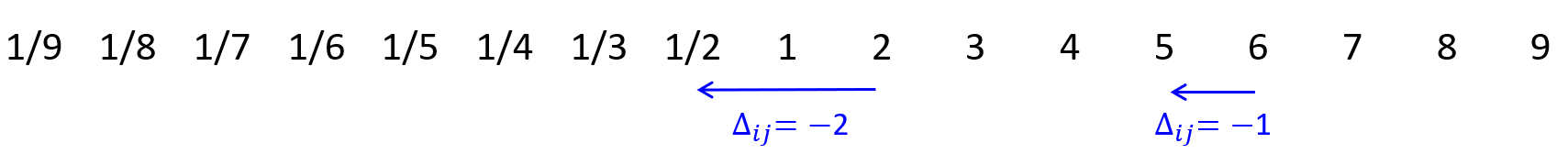
   Figure 9: The ratio scale $\boldsymbol{1/9,\ldots,9}$ and the perturbation of elements according to (9)–(11).

   Figure 10: The relation between CR and our element-wise perturbation via Box plots. Each Box plot is based on 1000 randomly generated perturbed PCMs.

3. We deleted the respective elements of the matrices in order to get the filling structure that we were examining, and applied the LLSM (and CREV in case of $n\leq 5$) technique(s) to obtain the weights. The certain models’ Euclidean distances and Kendall’s $\tau$ measures were computed with respect to the weights that were calculated from the complete inconsistent matrices. The analyzed filling in patterns included all of those that can be represented by connected non-isomorphic graphs with parameters $(n,e)$.

4. We repeated steps 1-3 for $1\ 000\ 000$ times for every level of inconsistency (thus altogether we examined $3\ 000\ 000$ PCMs for a given $(n,e)$ pair). Finally, we saved the mean of Euclidean distances and Kendall’s $\tau$ measures for the different filling in patterns.

Remark 4

The distribution of the elements of complete PCMs is independent of $n$. This property holds for both consistent and perturbed complete PCM cases.

This follows from the fact that in the simulations at first the elements of a given matrix are generated independently from $n$, and then they are placed into the $n\times n$ PCM. The histograms of the complete PCM elements above $1$ in the different perturbation cases, based on samples containing 1 million elements each, are presented in Figure 11 (with a 0.1 bin width).

Figure 11: The histograms of the $\geq 1$ elements of PCMs in case of different perturbations based on a sample of 1 million elements (with a 0.1 bin width).

According to the histograms, a higher level of perturbation (inconsistency) leads to a higher chance to have large (extreme) matrix elements.

apalike append

References

- Bernasconi et al., (2010) Bernasconi, M., Choirat, C., and Seri, R. (2010). The analytic hierarchy process and the theory of measurement. Management Science, 56(4):699–711. https://doi.org/10.1287/mnsc.1090.1123.
- Bozóki et al., (2010) Bozóki, S., Fülöp, J., and Rónyai, L. (2010). On optimal completion of incomplete pairwise comparison matrices. Mathematical and Computer Modelling, 52(1):318–333. https://doi.org/10.1016/j.mcm.2010.02.047.
- Bozóki et al., (2016) Bozóki, S., Csató, L., and Temesi, J. (2016). An application of incomplete pairwise comparison matrices for ranking top tennis players. European Journal of Operational Research, 248(1):211–218. https://doi.org/10.1016/j.ejor.2015.06.069.
- Csató and Rónyai, (2016) Csató, L. and Rónyai, L. (2016). Incomplete pairwise comparison matrices and weighting methods. Fundamenta Informaticae, 144(3-4):309–320. https://doi.org/10.3233/FI-2016-1337.
- Csató, (2013) Csató, L. (2013). Ranking by pairwise comparisons for Swiss-system tournaments. Central European Journal of Operations Research, 21(4):783–803. https://doi.org/10.1007/s10100-012-0261-8.
- Fedrizzi and Giove, (2007) Fedrizzi, M. and Giove, S. (2007). Incomplete pairwise comparison and consistency optimization. European Journal of Operational Research, 183(1):303–313. https://doi.org/10.1016/j.ejor.2006.09.065.
- Fedrizzi and Giove, (2013) Fedrizzi, M. and Giove, S. (2013). Optimal sequencing in incomplete pairwise comparisons for large dimensional problems. International Journal of General Systems, 42(4):366–375. https://doi.org/10.1080/03081079.2012.755523.
- Gass, (1998) Gass, S. (1998). Tournaments, transitivity and pairwise comparison matrices. Journal of the Operational Research Society, 49(6):616–624. https://doi.org/10.1057/palgrave.jors.2600572.
- Hashimoto and Nikkuni, (2013) Hashimoto, H. and Nikkuni, R. (2013). On Conway–Gordon type theorems for graphs in the Petersen family. Journal of Knot Theory and Its Ramifications, 22(9):1350048. https://doi.org/10.1142/S021821651350048X.
- Horvát, (2020) Horvát, Sz. (2020). IGraph/M. package for Wolfram Mathematica, https://github.com/szhorvat/IGraphM/tree/v0.4, https://doi.org/10.5281/zenodo.3739056.
- Kułakowski and Talaga, (2020) Kułakowski, K. and Talaga, D. (2020). Inconsistency indices for incomplete pairwise comparisons matrices. International Journal of General Systems, 49(2):174–200. https://doi.org/10.1080/03081079.2020.1713116.
- Lovász, (1977) Lovász, L. (1977). A homology theory for spanning trees of a graph. Acta Mathematica Academiae Scientiarum Hungaricae, 30(3-4):241–251. https://doi.org/10.1007/bf01896190.
- McKay and Piperno, (2014) McKay, B. D. and Piperno, A. (2014). Practical graph isomorphism, II. Journal of Symbolic Computation, 60(0):94–112. https://doi.org/10.1016/j.jsc.2013.09.003.
- Mesbahi, (2002) Mesbahi, M. (2002). On a dynamic extension of the theory of graphs. Proceedings of the 2002 American Control Conference (IEEE Cat. No.CH37301), 2:1234–1239. https://doi.org/10.1109/ACC.2002.1023188.
- Saaty, (1977) Saaty, T. L. (1977). A scaling method for priorities in hierarchical structures. Journal of Mathematical Psychology, 15(3):234–281. https://doi.org/10.1016/0022-2496(77)90033-5.
- Saaty, (1980) Saaty, T. L. (1980). The Analytic Hierarchy Process. McGraw-Hill, New York.
- Saw et al., (1984) Saw, J. G., Yang, M. C., and Mo, T. C. (1984). Chebyshev inequality with estimated mean and variance. The American Statistician, 38(2):130–132. https://doi.org/10.1080/00031305.1984.10483182.
- Steliga and Szynal, (2010) Steliga, K. and Szynal, D. (2010). On Markov-type inequalities. International Journal of Pure and Applied Mathematics, 58(2):137–152.
- (19) Szádoczki, Zs., Bozóki, S., Juhász, P., Kadenko, S. V., and Tsyganok, V. (2022a). Incomplete pairwise comparison matrices based on graphs with average degree approximately 3. Annals of Operations Research. https://doi.org/10.1007/s10479-022-04819-9.
- (20) Szádoczki, Zs., Bozóki, S., and Tekile, H. A. (2022b). Filling in pattern designs for incomplete pairwise comparison matrices: (Quasi-)regular graphs with minimal diameter. Omega, 107(C):102557. https://doi.org/10.1016/j.omega.2021.102557.
- Thurstone, (1927) Thurstone, L. (1927). A law of comparative judgment. Psychological Review, 34(4):273–286. https://doi.org/10.1037/h0070288.
- Triantaphyllou, (2000) Triantaphyllou, E. (2000). Multi-criteria decision making methods. In Multi-criteria Decision Making Methods: A Comparative Study. Applied Optimization, vol 44. Springer, Boston, MA. https://doi.org/10.1007/978-1-4757-3157-6_2.
- Wind and Saaty, (1980) Wind, Y. and Saaty, T. L. (1980). Marketing applications of the analytic hierarchy process. Management Science, 26(7):641–658. https://doi.org/10.1287/mnsc.26.7.641.
- Wolfram Research, (2021) Wolfram Research, I. (2021). Mathematica, Version 12.3. Champaign, IL, 2021. https://www.wolfram.com/mathematica.