Probing Lorentz-Invariance-Violation Induced Nonthermal Unruh Effect in Quasi-Two-Dimensional Dipolar Condensates

Abstract

The Unruh effect states an accelerated particle detector registers a thermal response when moving through the Minkowski vacuum, and its thermal feature is believed to be inseparable from Lorentz symmetry: Without the latter, the former disappears. Here we propose to observe analogue circular Unruh effect using an impurity atom in a quasi-two-dimensional Bose-Einstein condensate (BEC) with dominant dipole-dipole interactions between atoms or molecules in the ultracold gas. Quantum fluctuations in the condensate possess a Bogoliubov spectrum $\omega_{\mathbf{k}}=c_{0}|\mathbf{k}|f(\hbar\,c_{0}|\mathbf{k}|/M_{\ast})$, working as an analogue Lorentz-violating quantum field with the Lorentz-breaking scale $M_{\ast}$, and the impurity acts as an effective Unruh-DeWitt detector thereof. When the detector travels close to the sound speed, observation of the Unruh effect in our quantum fluid platform becomes experimentally feasible. In particular, the deviation of the Bogoliubov spectrum from the Lorentz-invariant case is highly engineerable through the relative strength of the dipolar and contact interactions, and thus a viable laboratory tool is furnished to experimentally investigate whether the thermal characteristic of Unruh effect is robust to the breaking of Lorentz symmetry.

Introduction.— One of the surprising fundamental consequences of relativistic quantum field theory is that the concept of particle number is observer dependent. A prominent paradigm is the so-called Unruh effect Unruh (1976): In the view of an uniformly accelerating observer, the Fock vacuum state of quantum field in the Minkowski spacetime appears as a thermal state rather than a zero-particle state. The corresponding characteristic temperature is proportional to the observer’s acceleration $a$, given by $k_{\text{B}}T_{\text{U}}=\frac{\hbar\,a}{2\pi\,c}$. To produce a measurable temperature for fundamental quantum fields, extremely huge accelerations are required (e.g., smaller than $1\,\mathrm{Kelvin}$ even for accelerations as high as $10^{20}\,\mathrm{m/s^{2}}$), and thus until now, the direct experimental confirmation of the Unruh effect still remains elusive.

Analogue gravity Unruh (1981); Barceló et al. (2011) opens up a new route to study various phenomenas predicted by relativistic quantum field theory, e.g., Hawking effect Garay et al. (2000); Nation et al. (2009); Lahav et al. (2010); Garay et al. (2000); Steinhauer (2014); Weinfurtner et al. (2011); Horstmann et al. (2010); Euvé et al. (2016); Steinhauer (2016); Roldán-Molina et al. (2017); Tian and Du (2019); Muñoz de Nova et al. (2019); Kolobov et al. (2021); Drori et al. (2019); Človečko et al. (2019); Kedem et al. (2020); Yang et al. (2020); Ribeiro et al. (2022); Tian et al. (2022), cosmological particle production Fedichev and Fischer (2004a); Hung et al. (2013); Prain et al. (2010); Fedichev and Fischer (2003); Alsing et al. (2005); Tian et al. (2017); Schützhold et al. (2007); Eckel et al. (2018); Lang and Schützhold (2019); Chä and Fischer (2017); Wittemer et al. (2019); Bhardwaj et al. (2021); Banik et al. (2022), and dynamical Casimir effect Johansson et al. (2009); Fujii et al. (2011); Wilson et al. (2011); Jaskula et al. (2012); Lähteenmäki et al. (2013); Macrì et al. (2018); Koghee and Wouters (2014); Dodonov (2020); Schneider et al. (2020), in a variety of electronic, acoustic, optical and even magnetic and superconducting settings. Recently, analogue gravity program for observing the Unruh effect has been successfully theoretically put forward Chen and Tajima (1999); Lochan et al. (2020); Schützhold et al. (2008); Retzker et al. (2008); Marino et al. (2020); Gooding et al. (2020); Sheng et al. (2021); Hegde et al. (2019); Zeng and Zubairy (2021); Cozzella et al. (2017); Barros et al. (2020); Guedes et al. (2019); Adjei et al. (2020), and through a BEC system Hu et al. experimentally realized the analogue Unruh effect relied on functional equivalence (i.e., simulating two-mode squeezed mechanics) Hu et al. (2019). Furthermore, in the quantum field theory, the contributions from the trans-Planckian modes as seen by an inertial observer are indispensable for deriving the Unruh effect with Bogoliubov transformation method. This particular feature makes the Unruh effect a potentially important arena for understanding and exploring implications of trans-Planckian physics Nicolini and Rinaldi (2011); Agulló et al. (2008); Hossain and Sardar (2015); Kajuri (2016); Hossain and Sardar (2016); Alkofer et al. (2016); Carballo-Rubio et al. (2019); Hammad et al. (2021); Louko and Upton (2018), and even the detecting means to probe some candidate theories of quantum gravity that may modify the trans-Planckian modes significantly. This modification usually accompanied by the breaking of Lorentz symmetry may even challenge the equivalence between Unruh effect and Hawking effect since the latter appears to be robust to high energy modifications of the dispersion relation Unruh (1995) while the former is not so immune and will lose its conventional thermal interpretation Nicolini and Rinaldi (2011); Agulló et al. (2008); Hossain and Sardar (2015, 2016); Carballo-Rubio et al. (2019) (see more details in the following). It is thus of great interest to experimentally investigate the consequences of trans-Planckian physics in a microscopically well-understood setup in a regime, that is inaccessible for quantum fields in real relativistic scenarios.

In this paper, we propose to study the interplay between the Unruh effect and trans-Planckian physics with an experimentally accessible platform consisting of a dipolar BEC Baranov (2008) and an immersed impurity Recati et al. (2005); Fedichev and Fischer (2003). From the perspective of analog, the density fluctuations in the condensate possessing trans-Planckian spectra leading to strong departures from Lorentz invariance Fischer (2006); Chä and Fischer (2017); Tian et al. (2018), resemble Lorentz-violating quantum field (LVQF), while the impurity, analogously dipole coupled to the density fluctuations, is modeled as an Unruh-DeWitt detector coupled to the LVQF. We will show that for the Lorentz-invariant (LI) spectrum the Unruh-DeWitt detector for an accelerated circular path indeed experiences a similar thermal response, while yields significant changes of this standard thermal feature when the spectra strongly deviate from Lorentz invariance. As far as we know, this represents the first example within analogue gravity where Unruh effect without thermality caused by the breaking of Lorentz symmetry can become experimentally manifest.

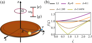
Figure 1: (a) A two-level atom immersed in a quasi-2D dipolar BEC, moving along a circular trajectory with the radius of the orbit $R$, an angular velocity $\Omega$ and the corresponding linear speed $v$. (b) The dimensionless function $f$ shown in (2) as a function of $\zeta=\hbar\,c_{0}k/M_{\ast}$. For the LI case, $f=1$. $R_{0}=0$ denotes the contact interaction case, where $f$ is independent of $A$. For DDI dominance, $R_{0}=\sqrt{\pi/2}$, $f$ dips below 1 for an interval of $\zeta$. Note that $f$ becomes negative when $A>A_{c}=3.4454$, which means the spectrum of quasiparticle becomes unstable.

Lorentz-violating quantum field and analogue Unruh-DeWitt detector in dipolar BEC.— As schematically shown in Fig. 1, we establish the connection between an impurity immersed in a quasi-two-dimensional (quasi-2D) dipolar BEC with the Unruh-DeWitt detector model Unruh (1976); Birrell and Davies , inspired by the seminal atomic quantum dot idea introduced in Refs. Recati et al. (2005); Fedichev and Fischer (2003, 2004b).

We begin with the Lagrangian density of an interacting Bose gas comprising atoms or molecules of mass $m$,

$$\mathcal{L} = \frac{i\hbar}{2}(\Psi^{\ast}\partial_{t}\Psi-\partial_{t}\Psi^{\ast}\Psi)-\frac{\hbar^{2}}{2m}|\nabla\Psi|^{2}-V_{\text{ext}}|\Psi|^{2}$$ (1)

$$-\frac{1}{2}|\Psi|^{2}\int\,d^{3}\mathbf{R}^{\prime}\,V_{\text{int}}(\mathbf{R}-\mathbf{R}^{\prime})|\Psi(\mathbf{R}^{\prime})|^{2},$$

where $\mathbf{R}=(\mathbf{r},z)$ are spatial 3D coordinates. The interaction reads $V_{\text{int}}(\mathbf{R}-\mathbf{R}^{\prime})=g_{c}\delta^{3}(\mathbf{R}-\mathbf{R}^{\prime})+3g_{d}\{[1-3(z-z^{\prime})^{2}/|\mathbf{R}-\mathbf{R}^{\prime}|^{2}]/|\mathbf{R}-\mathbf{R}^{\prime}|^{3}\}/4\pi$, where $g_{c}=4\pi\hbar^{2}a_{c}/m_{B}$ represents the contact interaction strength, with $a_{c}$ being the $s$-wave scattering length; the dipole-dipole interaction (DDI) strength $g_{d}=\mu_{0}\mu_{m}^{2}/3$, with $\mu_{0}$ and $\mu_{m}$ being the permeability of vacuum and the magnetic dipole moment that is polarized to the $z$ direction, respectively. Moreover, the gas is trapped by an external potential, $V_{\text{ext}}(\mathbf{R})=m_{B}\omega^{2}\mathbf{r}^{2}/2+m_{B}\omega^{2}_{z}z^{2}/2$, and is strongly confined along the $z$ axis, with aspect ratio $\kappa=\omega_{z}/\omega\gg 1$ over the whole time evolution. As a result of that, the motion of the Bose gas along the $z$ axis is frozen to the ground state with a Gaussian form, $\rho_{z}(z)=(\pi\,d^{2}_{z})^{-1/2}\exp[-z^{2}/d^{2}_{z}]$, with $d_{z}=\sqrt{\hbar/m_{B}\omega_{z}}$. Therefore, the whole system effectively reduces to a quasi-2D one which can ensure stability in the DDI-dominated regime Fischer (2006). Finally, we may assume that the Bose gas is condensed to the zero-momentum state with an area density $\rho_{0}$.

Within the Bogoliubov theory of small excitations on top of the condensate Pethick and Smith (2008); Pitaevskiĭ and Stringari (2016), density fluctuations in Heisenberg representation can be written as $\delta\hat{\rho}(t,\mathbf{r})=\sqrt{\rho_{0}}\int[d^{2}\mathbf{k}/(2\pi)^{2}](u_{\mathbf{k}}+v_{\mathbf{k}})[\hat{b}_{\mathbf{k}}(t)e^{i\mathbf{k}\cdot\mathbf{r}}+\hat{b}^{\dagger}_{\mathbf{k}}(t)e^{-i\mathbf{k}\cdot\mathbf{r}}]$ which closely resemble the quantum field in terms of bosonic operators $\hat{b}_{\mathbf{k}}(t)=\hat{b}_{\mathbf{k}}\,e^{-i\omega_{\mathbf{k}}\,t}$, satisfying the usual Bose commutation rules $[\hat{b}_{\mathbf{k}},\hat{b}_{\mathbf{k}^{\prime}}^{\dagger}]=(2\pi)^{2}\delta^{2}(\mathbf{k}-\mathbf{k}^{\prime})$. Note that $u_{\mathbf{k}}=(\sqrt{\mathcal{H}_{\mathbf{k}}}+\sqrt{\mathcal{H}_{\mathbf{k}}+2\mathcal{A}_{\mathbf{k}}})/2(\mathcal{H}^{2}_{\mathbf{k}}+2\mathcal{H}_{\mathbf{k}}\mathcal{A}_{\mathbf{k}})^{1/4}$ and $v_{\mathbf{k}}=(\sqrt{\mathcal{H}_{\mathbf{k}}}-\sqrt{\mathcal{H}_{\mathbf{k}}+2\mathcal{A}_{\mathbf{k}}})/2(\mathcal{H}^{2}_{\mathbf{k}}+2\mathcal{H}_{\mathbf{k}}\mathcal{A}_{\mathbf{k}})^{1/4}$ are Bogoliubov parameters, and the quasiparticle frequency $\omega_{\mathbf{k}}=\sqrt{\mathcal{H}^{2}_{\mathbf{k}}+2\mathcal{H}_{\mathbf{k}}\mathcal{A}_{\mathbf{k}}}$ with $\mathcal{H}_{\mathbf{k}}=k^{2}/2m$ and $\mathcal{A}_{\mathbf{k}}=\rho_{0}V^{\text{2D}}_{\text{int, 0}}(k)$ Tian et al. (2018). Here $k=|\mathbf{k}|$ and the Fourier transformation of DDI $V^{\text{2D}}_{\text{int, 0}}(k)=g^{\text{eff}}_{0}(1-\frac{3R_{0}}{2}kd_{z}w[\frac{kd_{z}}{\sqrt{2}}])$, with $w[x]=\exp[x^{2}](1-\operatorname{erf}[x])$, an effective contact coupling $g^{\text{eff}}_{0}=\frac{1}{\sqrt{2\pi}d_{z}}(g_{c}+2g_{d})$, and the dimensionless ratio $R_{0}=\sqrt{\pi/2}/(1+g_{c}/2g_{d})$. The parameter $R_{0}$ could be tunable via Feshbach resonance Courteille et al. (1998); Inouye et al. (1998); Chin et al. (2010); Timmermans et al. (1999) and rotating polarizing field Giovanazzi et al. (2002); Tang et al. (2018), ranging from $R_{0}=0$ (when $g_{d}/g_{c}\rightarrow 0$, i.e., contact dominance), to $R_{0}=\sqrt{\pi/2}$ (when $g_{d}/g_{c}\rightarrow\infty$, i.e., DDI dominance).

The density fluctuations described above closely resemble a LVQF with a explicit dispersion relation given by

$$\omega_{\mathbf{k}}=c_{0}k\sqrt{1-\frac{3R_{0}}{2}\sqrt{A}\zeta\,w\bigg{[}\sqrt{\frac{A}{2}}\zeta\bigg{]}+\frac{\zeta^{2}}{4}}=c_{0}kf(\zeta),$$ (2)

where $\zeta=\hbar\,c_{0}k/M_{\ast}$, $c_{0}=\sqrt{g^{\text{eff}}_{0}\rho_{0}/m_{B}}$ is the speed of sound, $A=g^{\text{eff}}_{0}\rho_{0}/\hbar\omega_{z}$ represents the effective chemical potential as measured relative to the transverse trapping, and $M_{\ast}=m_{B}c^{2}_{0}$ is the analog energy scale of Lorentz violation. This dispersion relation (2) is approximately Lorentz invariant $(f(\zeta)\simeq 1)$ for $\zeta\ll 1$. By appropriately setting the relevant parameters $A$ and $R_{0}$, the dispersion could be analogously superluminal $(f(\zeta)>1)$ and subluminal $(f(\zeta)<1)$. In Fig. 1, we plot the function $f(\zeta)$ shown in (2) to see how the Lorentz invariance is violated in this dispersion. For the DDI dominance, $R_{0}=\sqrt{\pi/2}$, the analogous subluminal spectrum develops a roton minimum for sufficiently large $A$, and the Lorentz invariance is strongly broken near $\zeta\simeq 0.9$ Tian et al. (2018).

In order to probe the analogue LVQF in the dipolar BEC, we use an impurity as the analogue Unruh-DeWitt detector, which consists of a two-level atom ($1$ and $2$) and its motion is supposed to be externally imposed by a tightly confining and relatively moving trap potential, so that its only degrees of freedom are the internal ones. Furthermore, the impurity is assumed to be controlled by a driving of a monochromatic external electromagnetic field at the frequency $\omega_{L}$ close to resonance with $1\rightarrow 2$ transition $\omega\simeq\omega_{21}$, with a Rabi frequency $\omega_{0}$. Then the Hamiltonian of the whole system can be written as

$$H(t) = \int\,d^{2}\mathbf{k}\hbar\omega_{\bf k}\hat{b}^{\dagger}_{\bf k}\hat{b}_{\bf k}+\hbar\omega_{21}|2\rangle\langle 2|-\bigg{(}\frac{\hbar\omega_{0}}{2}e^{-i\omega_{L}t}|2\rangle\langle 1|$$ (3)

$$+\mathrm{H.c.}\bigg{)}+\sum_{s=1,2}g_{s}\hat{\rho}(\mathbf{r}_{A}(t))|s\rangle\langle\,s|,$$

where the last term denotes the collisional coupling between the impurity and Bose gas, and $\hat{\rho}(\mathbf{r}_{A})=\hat{\psi}^{\dagger}(\mathbf{r}_{A})\hat{\psi}(\mathbf{r}_{A})\simeq\rho_{0}+\delta\hat{\rho}(\mathbf{r}_{A})$ represents the field density operator of the Bose gas with $\mathbf{r}_{A}(t)$ being the time-dependent position of the impurity.

In the rotated $|g,e\rangle=(|1\rangle\pm 2\rangle)/\sqrt{2}$ basis, the Rabi frequency $\omega_{0}$ determines the splitting between the $|g,e\rangle$ states, while the detuning $\delta=\omega_{L}-\omega_{21}$ gives a coupling terms. In such case, the impurity immersed in the condensate is collisionally coupled to the Bose gas via two channels Marino et al. (2017, 2020); Tian and Du (2021): The first term resembles the interaction of a static charge to an external scalar potential and can be canceled through proper tuning of the interaction constants $g_{1,2}$ (e.g., via Feshbach resonance Courteille et al. (1998); Inouye et al. (1998); Chin et al. (2010); Timmermans et al. (1999)), while the second term resembles a standard electric-dipole coupling. Choosing proper detuning $\delta$ to exactly compensate the coupling to the average density, we can finally find the impurity-fluctuations interaction Hamiltonian

$$H_{\text{int}}=g_{-}(e^{i\omega_{0}\tau}\sigma^{+}e^{-i\omega_{0}\tau}\sigma_{-})\delta\hat{\rho}({\bf r}_{A}(\tau),t_{A}(\tau)),$$ (4)

reproducing the usual Unruh-DeWitt detector-field interaction with $g_{-}=(g_{1}-g_{2})/2$ satisfying $\hbar\delta/2+g_{-}\rho_{0}=0$. However, here the LVQF is coupled to the detector.

Note that when $\zeta=\hbar\,c_{0}k/M_{\ast}\ll 1$ the density fluctuations resemble massless scalar field with spectrum, $\omega_{\mathbf{k}}\simeq\,c_{0}k$, the linearly moving impurity remains unexcited when its velocity satisfying $v<c_{0}$ , while behaves dramatically differently when moving at a supersonic speed $v\gtrsim\,c_{0}$. Specifically, although the “charge neutrality” of the impurity rules out Bogoliubov-Cherenkov emission Carusotto et al. (2006); Astrakharchik and Pitaevskii (2004), the anomalous Doppler effect may induce it to be excited from its ground state while emitting Bogoliubov phonon and still conserving energy. This is the analogue Ginzburg emission for superluminal moving particles Ginzburg and Frolov (1986); Ginzburg (1996), occurring in BEC. When the spectrum breaks the Lorentz symmetry satisfying $\omega_{\mathbf{k}}=c_{0}kf(\zeta)$: If $0<f(\zeta)<1$ for an interval of $\zeta$, the impurity would get excited when its velocity exceeds the critical $v_{c}=c_{0}f_{c}(\zeta)$ with $f_{c}(\zeta)=\inf\,f(\zeta)$ Tian and Du (2021). This particular property provides us a potential effective tool to constrain on the possible families of modified dispersion relations with the experimental results of the Relativistic Heavy Ion Collider Husain and Louko (2016). We will in the following consider a circularly moving impurity to observer the circular Unruh effect Bell and Leinaas (1983, 1987); Unruh (1998), and in particular examine whether the circular Unruh effect is robust to the breaking of Lorentz symmetry.

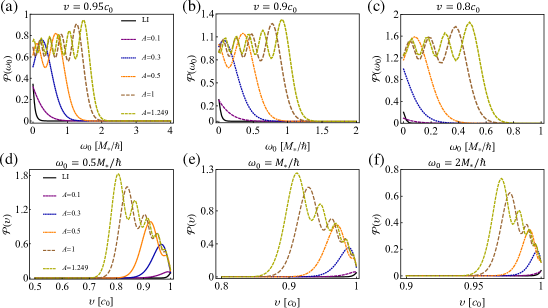
Figure 2: Transition rates shown in (5) for different effective chemical potential $A$, in units of $\frac{g^{2}_{0}\rho_{0}m_{B}}{2\hbar^{3}}$: (a), (b), (c) as a function of the detector’s energy spacing $\omega_{0}$ with fixed velocity; (d), (e), (f) as a function of the velocity $v$ with fixed energy spacing of the detector. Here we assume that the DDI dominance case ($R=\sqrt{\pi/2}$) is vailid.

Spontaneous excitation of the circularly moving detector.— If the detector moves with a circular trajectory $(c_{0}t(\tau),{\bf x}(\tau))=(c_{0}\gamma\tau,R\cos(\Omega\gamma\tau),R\sin(\Omega\gamma\tau),0)$, with constant radius $R$, the angular velocity $\Omega$, the usual relativistic factor $\gamma=1/\sqrt{1-R^{2}\Omega^{2}/c^{2}_{0}}$, and the corresponding acceleration $a=\Omega^{2}\gamma^{2}R$, we find the transition rate of the detector from its ground state to excited state Sup

$${\cal P}(\omega_{0}) = \frac{g^{2}_{-}\rho_{0}m_{B}}{2\hbar^{3}}\int^{\infty}_{0}d\zeta\frac{\zeta^{2}}{\gamma\,f(\zeta)}\sum^{\infty}_{m=-\infty}J^{2}_{m}(\tilde{M}\zeta)$$ (5)

$$\times \delta\bigg{(}\zeta\,f(\zeta)-\frac{1}{\tilde{M}}\bigg{(}mv-\frac{\tilde{E}}{\gamma}\bigg{)}\bigg{)},$$

where $\tilde{M}=RM_{\ast}/\hbar\,c_{0}$, $\tilde{E}=R\omega_{0}/c_{0}$, and $v=R\Omega/c_{0}$ are dimensionless parameters. Note that we focus on the detector’s speed in the preferred Lorentz frame satisfying $0\leq\,v<1$.

For the LI scenario where $R_{0}=0$ and $\omega_{\mathbf{k}}=c_{0}k\sqrt{1+\zeta^{2}/4}\approx\,c_{0}k$ for $k\ll\,k_{c}=M_{\ast}/c_{0}\hbar$, we find in the ultrarelativistic limit, $\gamma\gg 1$, the equilibrium population of the upper level relative to the lower is Sup

$$\frac{{\cal P}(\omega_{0})}{{\cal P}(-\omega_{0})}=\frac{12c^{2}_{0}\omega^{2}_{0}}{5a^{2}}\exp\big{(}-\sqrt{\frac{24}{5}}\frac{c_{0}\omega_{0}}{a}\big{)},$$ (6)

when the energy splitting of the detector is not too small $\omega_{0}\gg\,a/c_{0}$ Bell and Leinaas (1983), which leads to an effective temperature

$$T_{\text{eff}}=\frac{\sqrt{5}\hbar\,a}{2\sqrt{6}k_{B}c_{0}}.$$ (7)

This temperature is higher by a factor $\sqrt{5/6}\pi$ than the Unruh temperature for the linear acceleration, and higher by a factor $\sqrt{5/2}$ than the Unruh temperature for the real massless scalar field case as a result of the Bogoliubov transformation for the quasiparticles.

If $(\zeta\,f(\zeta))^{\prime}>0$, we can find in the limit, $\tilde{M}\rightarrow\infty$, the transition rate (5) behaves quite differently for $0<v<f_{c}$ and $f_{c}<v<1$, where $f_{c}=f(\zeta_{c})$ is a global minimum at $\zeta=\zeta_{c}>0$. Specifically, for the former, the transition rate ${\cal P}(\omega_{0})\rightarrow{\cal P}_{0}(\omega_{0})$, given by

$${\cal P}_{0}(\omega_{0})=\Gamma_{0}\sum^{\infty}_{m=\lceil\,\frac{\tilde{E}}{v\gamma}\rceil}\frac{1}{\gamma}\bigg{(}mv-\frac{\tilde{E}}{\gamma}\bigg{)}^{2}J^{2}_{m}\big{(}mv-\frac{\tilde{E}}{\gamma}\big{)},$$ (8)

where $\Gamma_{0}=\frac{g^{2}_{-}\rho_{0}}{2\hbar\,M_{\ast}\,R^{2}}$. Note this is the response for the analogue massless scalar field, and thus no low-energy Lorentz violation can been seen when $v<f_{c}$. While for the latter there is a correction to the former case, ${\cal P}(\omega_{0})\rightarrow{\cal P}_{0}(\omega_{0})+\Delta{\cal P}$, with

$$\Delta{\cal P}=\frac{g^{2}_{-}\rho_{0}m_{B}}{2\pi\hbar^{3}\gamma}\int^{\zeta_{+}}_{\zeta_{-}}d\zeta\frac{\zeta}{f(\zeta)\sqrt{v^{2}-f^{2}(\zeta)}},$$ (9)

where $\zeta_{-}\in(0,\zeta_{c})$ and $\zeta_{+}\in(\zeta_{c},\infty)$ are unique solutions to $f(\zeta)=v$ in the respective intervals. This correction means the detector sees a low-energy Lorentz violation when $v>f_{c}$, and alternatively the departure from the standard prediction of Unruh effect appears as a consequence of the Lorentz violation.

Experimental implementation.— Recent experimental advances have allowed for groundbreaking observations of strongly dipolar BEC, its excitation spectrum displaying roton minimum, and dynamics of impurity immersed in BEC Lu et al. (2011); Aikawa et al. (2012); Norcia et al. (2021); Chomaz et al. (2018); Petter et al. (2019); Schmidt et al. (2021); Natale et al. (2019); Hertkorn et al. (2021); Tomza et al. (2019); Weckesser et al. (2021); Skou et al. (2021); Dieterle et al. (2021). These experiments hold promise to realize our experimental scenario proposed above. Specifically, we can consider a single ${}^{87}\mathrm{Rb}$ atom immersed in a BEC of $\mathrm{Dy}$ atom Lu et al. (2011); Schmidt et al. (2021); Norcia et al. (2021) which possesses a magnetic dipole moment of $10\mu_{B}$ with $\mu_{B}$ being the Bohr magneton. The condensate density is assumed to be $\rho_{0}\sim 4.4\times 10^{3}\mathrm{\mu m}^{-2}$; The observer trajectory radius $R\sim 10\mathrm{\mu m}$; A typical trap frequency $\omega_{z}=2\pi\times 10^{3}\mathrm{Hz}$, the corresponding harmonic oscillator width is $d_{z}\simeq 0.25\times 10^{-6}\mathrm{m}$. Fig. 2 displays the transition rate in (5), and clearly shows the spontaneous excitation of the detector as a result of the circular acceleration in a Minkowski vacuum. This would be viewed as the circular Unruh effect: Thermal bath is predicted for an accelerated detector moving through the inertial vacuum. In addition, the transition rates clearly show the deviation from the LI field case, occurring for strongly dipolar interactions. Specifically, when the field slightly deviates from the LI case, e.g., $A=0.1$ case, their corresponding transition rates share similar behaviors. When this deviation becomes stronger, the excitation rates increase and behave sharply differently compared with the LI case, especially in the high velocity and low energy spacing regimes. However, for the low velocity case and large energy spacing of the detector, the excitation rates change slightly in the presence of Lorentz violation (i.e., they are not so sensitive to the breaking of Lorentz symmetry), since in such cases the detector is harder to excite.

To further check whether the Unruh effect is robust to the breaking of Lorentz symmetry, we naively define the Unruh temperature $T$ to estimate the fluctuations sampled by the impurity, using the Einstein’s detailed balanced condtion,

$$T=\hbar\omega_{0}k^{-1}_{B}\ln^{-1}\bigg{(}\frac{{\cal P}(-\omega_{0})}{{\cal P}(\omega_{0})}\bigg{)}.$$ (10)

This temperature is independent of $\omega_{0}$ for uniformly linearly accelerated detectors, given by $T_{\text{U}}=\frac{\hbar\,a}{2\pi\,k_{\text{B}}\,c}$, since whose response function satisfies the Kubo-Martin-Schwinger condition Kubo (1957); Martin and Schwinger (1959); Haag et al. (1967). For the circular acceleration cases, such definition of $T$ may depend on $\omega_{0}$, however, keeps monotonous increase via the effective acceleration parameter for the LI case Biermann et al. (2020). We here plot this temperature registered by the impurity coupled to the analogue LVQF as shown in Fig. 3. For the LI case, the temperature increases monotonously with the increase of the detector’s speed $v$ as expected. If the spectrum of the field deviates from the LI case slightly, e.g., $A=0.1$ case, the present temperature behaves similarly as the LI case but with a larger magnitude. Remarkably, when the spectra of the analogue LVQF strongly deviate from the LI spectrum, the temperature first increases with the increase of the detector’s speed and then oscillates if the detector’s speed exceeds a critical value which depends on the degree of the deviation. The counterintuitive oscillation phenomenon means that Lorentz violation may break the thermal characteristic of Unruh effect, and even cause the analogue anti-Unruh effect Brenna et al. (2016): Unruh temperature decreases with the increase of acceleration. Besides, the effective negative temperature Purcell and Pound (1951); Ramsey (1956) occurs during the oscillation, which implies that as a result of Lorentz violation, the corresponding detector’s state is characterized by an inverted occupation distribution, where excited state is populated more than ground state.

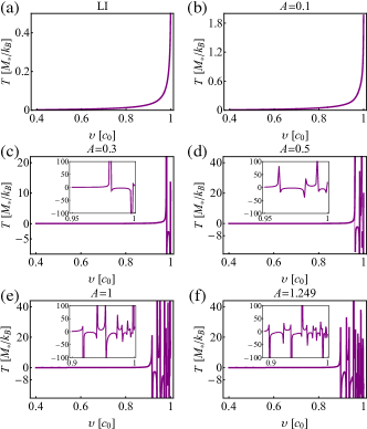
Figure 3: The temperature defined in (10) as a function of the detector’s velocity $v$ with fixed energy spacing of the detector, $\omega_{0}=M_{\ast}/\hbar$. Insets are the details of the corresponding oscillation parts. Here we assume that the DDI dominance case ($R=\sqrt{\pi/2}$) is vailid.

Conclusions.— We present a concrete experimental proposal to test how the Lorentz violation affects the circular Unruh effect using an impurity immersed in a dipolar BEC. We find that if the spectra of quantum field deviate from the LI case strongly, the transition rates and the predicted temperature of the analogue Unruh-DeWitt detector behave quite differently compared with the LI case, and the Lorentz violation even more may induce the counter-intuitive anti-Unruh effect on certain conditions. Our preliminary estimates indicate that the proposed experimental implementation of the analogue circular Unruh effect and its interaction with the Lorentz-breaking physics is within reach of current state-of-the-art ultracold-atom experiments.

Our proposed quantum fluid platform may also allow us in the experimentally accessible regime to explore open questions concerning Unruh effect Retzker et al. (2008), and why its robustness to high energy modifications of the dispersion relation Carballo-Rubio et al. (2019) behaves differently from that of its equivalence principle dual—Hawking effect Unruh (1995). In addition, two impurities could be used as detectors to explore correlations harvest from the quantum vacuum of analogue quantum fields Pozas-Kerstjens and Martín-Martínez (2015).

Supplementary Material

I Unruh effect of accelerated detector

We here simply review the Unruh effect corresponding to the linear acceleration and circular motion cases. In quantum field theory, usually quantum field is probed with a linearly coupled Unruh-DeWitt detector Unruh (1976); Birrell and Davies , which is described by a localized system with internal levels $|g\rangle$ and $|e\rangle=\sigma^{+}|g\rangle$ and the energy gap $\omega_{0}$, moving along a trajectory $(t(\tau),{\bf x}(\tau))$ with $\tau$ being the detector’s proper time. The detector couples with a scalar field $\phi$, initially in its vacuum state, through

$$H_{\text{int}}=g\chi(\tau)(e^{i\omega_{0}\tau}\sigma^{+}e^{-i\omega_{0}\tau}\sigma_{-})\phi({\bf x}(\tau),t(\tau)),$$ (S1)

where $g$ is the coupling parameter and $\chi(\tau)$ is a real-valued smooth switching function that specifies how the interaction is turned on and off. In the first-order perturbation theory, the probability for the detector to be excited from its ground $|g\rangle$ to the excited state $|e\rangle$ is proportional to the response function,

$${\cal F}(\omega_{0})=\frac{g^{2}}{\hbar^{2}}\int\int\,d\tau\,d\tau^{\prime}\chi(\tau)\chi(\tau^{\prime})e^{-i\omega_{0}(\tau-\tau^{\prime})}{\cal W}(\tau,\tau^{\prime}),$$

where ${\cal W}(\tau,\tau^{\prime})=\langle 0|\phi(t(\tau),{\bf x}(\tau))\phi(t(\tau^{\prime}),{\bf x}(\tau^{\prime}))|0\rangle$ denotes the Wightman function evaluated along the detector’s trajectory. If we consider the scenario where the detectors’s trajectories and quantum field state are stationary, in this sense that ${\cal W}(\tau,\tau^{\prime})$ depends on its arguments only through the difference $s=\tau-\tau^{\prime}$. We may then calculate the transition probability per unit time (or the transition rate) by dividing ${\cal F}(\omega_{0})$ with respective to the total interaction time and letting this interaction time tend to infinity, finally find

$${\cal P}(\omega_{0})={\cal F}_{\text{rate}}(\omega_{0})=\frac{g^{2}}{\hbar^{2}}\int_{-\infty}^{\infty}\,ds\,e^{-i\omega_{0}s}{\cal W}(s,0).$$ (S2)

Note (S2) denotes the excitation rate from the detector’s ground state to its excited state.

The Wightman function for a massless scalar field in Minkowski spacetime is analytically ${\cal W}(\tau,\tau^{\prime})=-\frac{\hbar\,c_{0}}{4\pi^{2}}\frac{1}{(c_{0}t(\tau)-c_{0}t^{\prime}(\tau^{\prime}))^{2}-({\bf x}(\tau)-{\bf x}^{\prime}(\tau^{\prime}))^{2}}$. For the linearly accelerated trajectory, $x(\tau)=\frac{c^{2}_{0}}{a}\cosh\frac{a\tau}{c_{0}},t(\tau)=\frac{c_{0}}{a}\sinh\frac{a\tau}{c_{0}}$, it reduces to

$${\cal W}_{l}(\tau,\tau^{\prime}) = -\frac{a^{2}\hbar}{16\pi^{2}c^{3}_{0}}\bigg{\{}\sinh\bigg{[}\frac{a}{2c_{0}}(\tau-\tau^{\prime})\bigg{]}\bigg{\}}^{-2}$$ (S3)

$$= -\frac{\hbar}{4\pi^{2}c_{0}}(\tau-\tau^{\prime})^{-2}\bigg{(}1+\frac{1}{12}\bigg{[}\frac{a}{c_{0}}(\tau-\tau^{\prime})\bigg{]}^{2}+\frac{1}{360}\bigg{[}\frac{a}{c_{0}}(\tau-\tau^{\prime})\bigg{]}^{4}+\dots\bigg{)}^{-1}.$$

Together with (S2), one can find that the accelerated detector becomes thermalized with the transition probabilities satisfying ${\cal P}_{\text{excitation}}/{\cal P}_{\text{de-excitation}}={\cal P}(\omega_{0})/{\cal P}(-\omega_{0})=e^{-\hbar\omega_{0}/k_{\text{B}}T_{\text{U}}}$, where $T_{\text{U}}=\frac{\hbar\,a}{2\pi\,c_{0}k_{B}}$ is the Unruh temperature. Note that observation of Unruh effect in the practice remains a challenged problem because of the extreme requirement of high linearly acceleration for typical detector’s transition.

Going beyond the linear acceleration scenario, the circular motion with a constant radial acceleration could also produce an approximately thermal spectrum Bell and Leinaas (1983, 1987); Unruh (1998), presenting the circular Unruh effect. Specifically, if the detector moves along a circular trajectory $(c_{0}t(\tau),{\bf x}(\tau))=(c_{0}\gamma\tau,R\cos(\Omega\gamma\tau),R\sin(\Omega\gamma\tau),0)$, with constant radius $R$, the usual relativistic factor $\gamma=(1-v^{2}/c^{2}_{0})^{-1/2}=(1-\beta^{2})^{-1/2}$, the angular velocity $\Omega=v/R$ and the corresponding acceleration $a=v^{2}\gamma^{2}/R=\Omega^{2}\gamma^{2}R$, one can find the corresponding Wightman function

$${\cal W}_{c}(\tau,\tau^{\prime}) = -\frac{\hbar}{4\pi^{2}c_{0}}\bigg{\{}\gamma^{2}(\tau-\tau^{\prime})^{2}-\bigg{(}2\frac{c_{0}}{a}\beta^{2}\gamma^{2}\bigg{)}^{2}\bigg{(}\sin\bigg{[}\frac{a}{2c_{0}}\frac{\tau-\tau^{\prime}}{\beta\gamma}\bigg{]}\bigg{)}^{2}\bigg{\}}^{-1}$$ (S4)

$$= -\frac{\hbar}{4\pi^{2}c_{0}}(\tau-\tau^{\prime})^{-2}\bigg{(}1+\frac{1}{12}\bigg{[}\frac{a}{c_{0}}(\tau-\tau^{\prime})\bigg{]}^{2}-\frac{1}{360\beta^{2}\gamma^{2}}\bigg{[}\frac{a}{c_{0}}(\tau-\tau^{\prime})\bigg{]}^{4}+\dots\bigg{)}^{-1}.$$

Comparing the Wightman function (S4) with (S3), there is distinct difference: an extra parameter, $\beta$ or $\gamma$, appears in the circular motion case. This is because for circular motion the radius of the circle can be varied independently of the acceleration. Unlike the linear accelerated case, the Fourier transformation of (S4) is not analytical. However, it, in the ultrarelativistic limit, $\gamma\gg 1$, can be simplified. Then the corresponding equilibrium transition probabilities yields Bell and Leinaas (1983)

$$\frac{{\cal P}_{\text{excitation}}}{{\cal P}_{\text{de-excitation}}}\approx\frac{a}{4\sqrt{3}\omega_{0}c_{0}}e^{-2\sqrt{3}\frac{\omega_{0}c_{0}}{a}}$$ (S5)

for the $a/c_{0}\omega_{0}\ll 1$ case. It leads to an effective temperature $T_{\text{eff}}=\frac{\hbar\,a}{2\sqrt{3}k_{B}c_{0}}$, which is higher by a factor $\pi/\sqrt{3}$ than the Unruh temperature for the linear acceleration.

Note that compared with the linear acceleration case, circular motion allows the accelerating system to remain within a finite-size laboratory for an arbitrarily long interaction time. Furthermore, unlike what happens in uniform linear acceleration, the proper and coordinate time for the circular motion are related by a time-independent gamma faction, which will be crucial when estimating the experimental feasibility for detecting the analogue circular Unruh effect.

II Derivation of the transition rate

The density fluctuations of dipolar BEC is of the form,

$$\delta\hat{\rho}(t,\mathbf{r})=\sqrt{\rho_{0}}\int\frac{d^{2}\mathbf{k}}{(2\pi)^{2}}(u_{\mathbf{k}}+v_{\mathbf{k}})\big{[}\hat{b}_{\mathbf{k}}(t)e^{i\mathbf{k}\cdot\mathbf{r}}+\hat{b}^{\dagger}_{\mathbf{k}}(t)e^{-i\mathbf{k}\cdot\mathbf{r}}\big{]}.$$ (S6)

We can use it to calculate the analogue correlation function of the density fluctuations

$$\langle 0|\delta\hat{\rho}(t,\mathbf{r})\delta\hat{\rho}(t^{\prime},\mathbf{r}^{\prime})|0\rangle = \frac{\rho_{0}}{(2\pi)^{4}}\int\int\,d^{2}\mathbf{k}\,d^{2}\mathbf{k}^{\prime}(u_{k}+v_{k})(u_{k^{\prime}}+v_{k^{\prime}})\langle 0|\big{[}\hat{b}_{\mathbf{k}}(t)e^{i\mathbf{k}\cdot\mathbf{r}}+\mathrm{h.c.}\big{]}\big{[}\hat{b}_{\mathbf{k}^{\prime}}(t^{\prime})e^{i\mathbf{k}^{\prime}\cdot\mathbf{r}^{\prime}}+\mathrm{h.c.}\big{]}|0\rangle$$ (S7)

$$= \frac{\rho_{0}}{(2\pi)^{2}}\int\int\,d^{2}\mathbf{k}\,d^{2}\mathbf{k}^{\prime}(u_{k}+v_{k})(u_{k^{\prime}}+v_{k^{\prime}})e^{-i\omega_{\mathbf{k}}\,t+i\omega_{\mathbf{k}^{\prime}}t^{\prime}}e^{i\mathbf{k}\cdot\mathbf{r}-i\mathbf{k}^{\prime}\cdot\mathbf{r}^{\prime}}\delta^{2}(\mathbf{k}-\mathbf{k}^{\prime})$$

$$= \frac{\rho_{0}}{(2\pi)^{2}}\int\,d^{2}\mathbf{k}(u_{k}+v_{k})^{2}e^{-i\omega_{\mathbf{k}}(t-t^{\prime})}e^{i\mathbf{k}\cdot(\mathbf{r}-\mathbf{r}^{\prime})}$$

$$= \frac{\rho_{0}}{(2\pi)^{2}}\int^{\infty}_{0}dk\int^{2\pi}_{0}d\theta\,k(u_{k}+v_{k})^{2}e^{-i\omega_{\mathbf{k}}(t-t^{\prime})}e^{i|\mathbf{k}||\mathbf{r}-\mathbf{r}^{\prime}|\cos\theta}$$

$$= \frac{\rho_{0}}{(2\pi)}\int^{\infty}_{0}dk\,k(u_{k}+v_{k})^{2}e^{-i\omega_{\mathbf{k}}(t-t^{\prime})}J_{0}\big{(}|\mathbf{k}||\mathbf{r}-\mathbf{r}^{\prime}|\big{)},$$

where $J_{0}(x)$ is the Bessel function of the first kind. For the uniform circular motion case, the trajectory is $(t(\tau),\mathbf{r}(\tau))=(\gamma\tau,R\cos(\gamma\Omega\tau),R\sin(\gamma\Omega\tau))$, and it is easy to find $t-t^{\prime}=\gamma(\tau-\tau^{\prime})=\gamma\,s$ and $|\mathbf{r}-\mathbf{r}^{\prime}|=2R\sin\frac{\gamma\Omega}{2}s$. Inserting this trajectory into the above correlation function of the density fluctuations, we can calculate the transition rate

$${\cal P}(\omega_{0}) = \frac{g^{2}_{-}\rho_{0}}{2\pi\hbar^{2}}\int\,ds\int^{\infty}_{0}dk\,k(u_{k}+v_{k})^{2}J_{0}\bigg{(}2Rk\sin\frac{\gamma\Omega}{2}s\bigg{)}e^{-i(\omega_{0}+\gamma\omega_{\mathbf{k}})s}$$ (S8)

$$= \frac{g^{2}_{-}\rho_{0}}{2\pi\hbar^{2}}\int\,ds\int^{\infty}_{0}dk\,k(u_{k}+v_{k})^{2}\sum^{\infty}_{m=-\infty}J^{2}_{m}(Rk)e^{im\gamma\Omega\,s}e^{-i(\omega_{0}+\gamma\omega_{\mathbf{k}})s}$$

$$= \frac{g^{2}_{-}\rho_{0}}{\hbar^{2}\gamma}\int^{\infty}_{0}dk\,k(u_{k}+v_{k})^{2}\sum^{\infty}_{m=-\infty}J^{2}_{m}(Rk)\delta\big{(}\frac{\omega_{0}}{\gamma}+\omega_{\mathbf{k}}-m\Omega\big{)}$$

$$= \frac{g^{2}_{-}\rho_{0}m_{B}}{2\hbar^{3}}\int^{\infty}_{0}d\zeta\frac{\zeta^{2}}{\gamma\,f(\zeta)}\sum^{\infty}_{m=-\infty}J^{2}_{m}(\tilde{M}\zeta)\delta\bigg{(}\zeta\,f(\zeta)-\frac{1}{\tilde{M}}\bigg{(}mv-\frac{\tilde{E}}{\gamma}\bigg{)}\bigg{)},$$

where $\zeta=\hbar\,c_{0}k/M_{\ast}$, $\tilde{M}=RM_{\ast}/\hbar\,c_{0}$, $\tilde{E}=R\omega_{0}/c_{0}$, and $v=R\Omega/c_{0}$ are dimensionless parameters. Note that to derive the second equality the identity, $J_{0}(2a\sin\,x)=\sum_{m\in\mathbf{Z}}J^{2}_{m}(a)e^{2imx}$, has been used.

II.1 Thermal circular Unruh effect

If $R_{0}=0$, it means only contact interaction happens between atoms or molecules in Bose gas, we can find the excitation spectrum has the form, $\omega_{\mathbf{k}}=c_{0}k\sqrt{1+\zeta^{2}/4}$, which is “relativistic” Retzker et al. (2008). $\omega_{\mathbf{k}}\approx\,c_{0}k$, for $k\ll\,k_{c}=M_{\ast}/c_{0}\hbar$. Then, (S8) reduces to,

$${\cal P}(\omega_{0}) = \frac{g^{2}_{-}\rho_{0}}{2\pi\hbar^{2}}\int\,ds\int^{\infty}_{0}dk\,k(u_{k}+v_{k})^{2}J_{0}\bigg{(}2Rk\sin\frac{\gamma\Omega}{2}s\bigg{)}e^{-i(\omega_{0}+\gamma\omega_{\mathbf{k}})s}$$ (S9)

$$= \frac{g^{2}_{-}\rho_{0}}{2\pi\hbar^{2}}\int\,ds\int^{\infty}_{0}dk\,k\frac{\hbar^{2}k^{2}/2m_{B}}{\hbar\,c_{0}k}J_{0}\bigg{(}2Rk\sin\frac{\gamma\Omega}{2}s\bigg{)}e^{-i\gamma\,c_{0}ks}e^{-i\omega_{0}s}$$

$$= \frac{g^{2}_{-}\rho_{0}}{4\pi\hbar\,m_{B}c_{0}}\int\,ds\int^{\infty}_{0}dk\,k^{2}J_{0}\bigg{(}2Rk\sin\frac{\gamma\Omega}{2}s\bigg{)}e^{-i\gamma\,c_{0}ks}e^{-i\omega_{0}s}$$

$$= \frac{g^{2}_{-}\rho_{0}}{4\pi\hbar\,m_{B}c_{0}}\int\,ds\frac{-2\gamma^{2}c^{2}_{0}s^{2}-4R^{2}\sin^{2}\frac{\gamma\Omega}{2}s}{\big{(}-\gamma^{2}c^{2}_{0}s^{2}+4R^{2}\sin^{2}\frac{\gamma\Omega}{2}s\big{)}^{5/2}}e^{-i\omega_{0}s}.$$

In the ultrarelativistic limit, $\gamma\gg 1$, we can do the same process as in Bell and Leinaas (1983) to further calculate the above transition rate, which is given by

$${\cal P}(\omega_{0}) = \frac{g^{2}_{-}\rho_{0}}{4\pi\hbar\,m_{B}c_{0}}\int\,ds\frac{24i(-1+3\gamma^{2})}{24c^{3}_{0}s^{3}+5a^{2}c_{0}s^{5}}e^{-i\omega_{0}s}$$ (S10)

$$= \frac{5g^{2}_{-}\rho_{0}}{96\sqrt{2\pi}\hbar\,m_{B}c^{6}_{0}}(3\gamma^{2}-1)a^{2}\bigg{[}1-\exp\big{(}-\sqrt{\frac{24}{5}}\frac{c_{0}\omega_{0}}{a}\big{)}+\frac{12c^{2}_{0}\omega^{2}_{0}}{5a^{2}}\bigg{]}.$$

Furthermore, assuming the energy splitting of the detector to be not too small $\omega_{0}\gg\,a/c_{0}$, we can find the equilibrium population of the upper level relative to the lower is

$$\frac{{\cal P}(\omega_{0})}{{\cal P}(-\omega_{0})}=\frac{12c^{2}_{0}\omega^{2}_{0}}{5a^{2}}\exp\big{(}-\sqrt{\frac{24}{5}}\frac{c_{0}\omega_{0}}{a}\big{)},$$ (S11)

leading to an effective temperature

$$T_{\text{eff}}=\frac{\sqrt{5}\hbar\,a}{2\sqrt{6}k_{B}c_{0}}.$$ (S12)

II.2 Correction to the LI case

As shown above, the transition rate of the detector from its ground state to excited state is

$${\cal P}(\omega_{0})=\frac{g^{2}_{-}\rho_{0}m_{B}}{2\hbar^{3}}\int^{\infty}_{0}d\zeta\frac{\zeta^{2}}{\gamma\,f(\zeta)}\sum^{\infty}_{m=-\infty}J^{2}_{m}(\tilde{M}\zeta)\delta\bigg{(}\zeta\,f(\zeta)-\frac{1}{\tilde{M}}\bigg{(}mv-\frac{\tilde{E}}{\gamma}\bigg{)}\bigg{)},$$ (S13)

where $\tilde{M}=RM_{\ast}/\hbar\,c_{0}$, $\tilde{E}=R\omega_{0}/c_{0}$, and $v=R\Omega/c_{0}$ are dimensionless parameters.

We consider the stable dipolar BEC and thus $f(\zeta)$ is smooth and strictly positive, and $f(\zeta)\rightarrow 1$ as $\zeta\rightarrow 0$. We also consider the scenario where the only stationary point of $f$ is a global minimum at $g=g_{c}>0$, written as $f_{c}=f(g_{c})$ with $0<f_{c}<1$. In such case, $f^{\prime}(\zeta)<0$ for $0<\zeta<\zeta_{c}$ and $f^{\prime}(\zeta)>0$ for $\zeta>\zeta_{c}$. In addition to that, we also assume that $\zeta\,f(\zeta)$ is a monotonely increasing function of $\zeta$, which means $(\zeta\,f(\zeta))^{\prime}=\zeta\,f^{\prime}(\zeta)+f(\zeta)>0$ for $\zeta>0$. Then we can perform the integral in Eq. (S13), and find

$${\cal P}(\omega_{0})=\frac{g^{2}_{-}\rho_{0}m_{B}}{2\hbar^{3}\gamma}\sum^{\infty}_{m=\lceil\,\frac{\tilde{E}}{v\gamma}\rceil}\frac{\zeta^{2}_{m}/f(\zeta_{m})}{(\zeta\,f(\zeta))^{\prime}|_{\zeta=\zeta_{m}}}J^{2}_{m}(\tilde{M}\zeta_{m}),$$ (S14)

where $\zeta_{m}$ is the unique solution to $\zeta\,f(\zeta)=\frac{1}{\tilde{M}}\big{(}mv-\frac{\tilde{E}}{\gamma}\big{)}$. In the limit $\tilde{M}\rightarrow\infty$, we find that the limit is qualitatively different for $0<v<f_{c}$ and $f_{c}<v<1$, as found in Refs. Louko and Upton (2018):

$${\cal P}_{0}(\omega_{0})=\frac{g^{2}_{-}\rho_{0}}{2\hbar\,M_{\ast}\,R^{2}\gamma}\sum^{\infty}_{m=\lceil\,\frac{\tilde{E}}{v\gamma}\rceil}\bigg{(}mv-\frac{\tilde{E}}{\gamma}\bigg{)}^{2}J^{2}_{m}\big{(}mv-\frac{\tilde{E}}{\gamma}\big{)},$$ (S15)

for the $0<v<f_{c}$ case. Note that in this case the detector sees no low-energy Lorentz violation: the corresponding response is the same as that for the usual massless scalar field. For $f_{c}<v<1$, ${\cal P}(\omega_{0})\rightarrow{\cal P}_{0}(\omega_{0})+\Delta{\cal P}$ as $\tilde{M}\rightarrow\infty$, where

$$\Delta{\cal P}=\frac{g^{2}_{-}\rho_{0}m_{B}}{2\pi\hbar^{3}\gamma}\int^{\zeta_{+}}_{\zeta_{-}}d\zeta\frac{\zeta}{f(\zeta)\sqrt{v^{2}-f^{2}(\zeta)}},$$ (S16)

and $\zeta_{-}\in(0,g_{c})$ and $\zeta_{+}\in(g_{c},\infty)$ are unique solutions to $f(\zeta)=v$ in the respective intervals.

Note that when $v>f_{c}$ and $\tilde{M}$ is large, the Lorentz-breaking contribution to the sum in Eq. (S14) comes from values of $m$ that are comparable to $\tilde{M}$. In conclusion, Lorentz violation of quantum fields would affect the transition rate of the Unruh-DeWitt detector: The detector in circular motion in the preferred inertial frame sees a large low-energy Lorentz violation when its orbital speed exceeds the critical value $f_{c}$.